跳到论文正文
W Papers独立论文阅读器 arXiv:1704.06385 论文正文 计算阅读时间 · 0%
引用这篇论文根据当前论文元数据生成,正式投稿前建议核对。


License: arXiv.org perpetual non-exclusive license
arXiv:1704.06385v1 [math.DG] 21 Apr 2017

Ricci flow recovering from pinched discsThanks: The author has been partially supported by the NSF grant DMS 1148490.

Tim Carson Timothy CarsonUniversity of Texas, Department of Mathematics
2515 Speedway stop C1200
Austin, Texas 78712-1202
Abstract.

We construct smooth solutions to Ricci flow starting from a class of singular metrics and give asymptotics for the forward evolution. The singular metrics heal with a set of points (of codimension at least three) coming out of the singular point. We conjecture that these metrics arise as final-time limits of Ricci flow encountering a Type-I singularity modeled on p+1×Sq\real{}^{p+1}\times S^{q}. This gives a picture of Ricci flow through a singularity, in which a neighborhood of the manifold changes topology from Dp+1×SqD^{p+1}\times S^{q} to Sp×Dq+1S^{p}\times D^{q+1} (through the cone over Sp×SqS^{p}\times S^{q}.)

We work in the class of doubly-warped product metrics. We also briefly discuss some possible smooth and non-smooth forward evolutions from other singular initial data.

0.1. Description of a flow through a singularity

In this paper we prove the existence of, and provide asymptotics for, Ricci flow starting from certain singular initial metrics. We believe that these singular initial metrics can arise as limits of Ricci flow with a finite-time singularity, in a way described by Hamilton in [Ham95]. We also provide formal arguments for the asymptotics of the flow into the singularity.

The flow through the singularity is illustrated in Figure 1. Take (Np+1,gN)(N^{p+1},g_{N}) to be a manifold with small curvature, and now consider a metric on N×SqN\times S^{q} (q≥2q\geq 2) obtained by placing a sphere of some size on every point in NN. After running Ricci flow for a short time, the spheres’ sizes obey a reaction-diffusion equation while the metric on NN also changes. If we make the initial spheres on NN small in some region, we can force a singularity to occur in that region, at one point on NN. The singularity will be modeled on Rp+1×SqR^{p+1}\times S^{q} if the Np+1N^{p+1} factor stays relatively smooth. Near the singularity point but before the singular time the manifold has a region with topology Dp+1×SqD^{p+1}\times S^{q}. At the singular time this region takes on the topology of the cone over Sp×SqS^{p}\times S^{q} (but is not close to a metric cone).

Afterwards, the SpS^{p} factor grows, and the manifold takes on the topology of Sp×Dq+1S^{p}\times D^{q+1} near the singularity. The case p=0p=0 is the well known standard neckpinch case, see Figure 2. A somewhat disappointing aspect of this topological change is that if p≥2p\geq 2 then Ricci flow can perform the opposite topological change (by reversing the roles of pp and qq in the description above.)

Refer to caption
Figure 1. A neighborhood of a doubly warped product undergoing Ricci flow. Initially, the neighborhood has topology D2×S2D^{2}\times S^{2}. The size of the S2S^{2} at the center of the D2D^{2} is quite small. In the middle, the flow has reached a singularity. The neighborhood has the topology of the cone over S1×S2S^{1}\times S^{2}. The flow continues on the right. The manifold is again smooth and the neighborhood has topology S1×D3S^{1}\times D^{3}. The size of the inner circle is relatively large compared to the curvature of the S2S^{2} factor near the inside. In a rescaling going backwards in time the manifold will converge to (×Steady Bryant Soliton)(\real\times\text{Steady Bryant Soliton}).
Refer to caption
Figure 2. A doubly warped product over an interval with fibers S0S^{0} and S2S^{2} undergoing Ricci flow. Some S0S^{0}’s are marked with pairs of cubes. Having an S0S^{0} fiber is somewhat equivalent to asking for the size of the S2S^{2} in a singly warped product to be an even function. As far as intrinsic metric spaces are concerned there is no size of the S0S^{0} factor (i.e. if p=0p=0 the function ψ\psi has no effect.) If we were considering mean curvature flow, the size of the S0S^{0} factor could be understood as the distance between the two disconnected parts after a neckpinch.

0.2. Forward evolutions from singular metrics

Our work continues the investigation into which singular metrics have a forward Ricci flow which smooths them. A usual method to construct such flows (which we use) is to consider the Ricci flow from smooth metrics approximating the initial metric. If these smooth mollifications of the initial metric have uniform short time existence, then one can extract a limiting flow as the modification goes to zero.

We work within the class of doubly warped product metrics, which simplifies the Ricci flow equation to a system of parabolic equations on an interval. The authors of [ACK12] and [Car16] similarly construct flows starting from singular initial data, but in the case of a singly warped product over an interval. As with our work, the motivation was to understand certain flows through singularities. The singular initial metrics considered there arise from singularities modeled on ×Sq\real\times S^{q} which are type I and type II, respectively.

In three dimensions, Ricci flow through singularities is now well understood. Kleiner and Lott [KL14] show that Perelman’s Ricci flow with surgery [Per03] can be seen as an approximation to a true flow with some singularities occurring and healing. One result of [KL14] is that such a flow through singularities in three dimensions has finitely many “bad worldlines”, so intuitively speaking only finitely many points come out of singularities. (E.g. the two cubes marking the inner S0S^{0} in the third part of Figure 2.) It is unsurprising that this should be false in higher dimensions, since the proof comes from a classification of possible ways a singularity can heal. To our knowledge we can hope for a statement about the codimension of such points. (In our examples they have codimension three or more.)

In [GS16], Gianniotis and Schulze construct flows starting from singular metrics without any symmetry assumptions. Their initial metrics have isolated singular points modeled on non-negatively curved cones over SnS^{n}. These are conjectured to arise as final time limits of type-I singularities, when the shrinking soliton which the singularity is modeled on is asymptotically Ricci flat. The metrics immediately heal, using expanding solitons which are asymptotic to the cones (shown to exist by Deruelle [Der16]).

The examples from [GS16] heal with an expander with scale t\sqrt{t}, whereas the examples here, in [ACK12], and in [Car16] heal at a smaller scale. In all of these examples if for the initial metric, |Rm|2=O(γ(d);d↘0)|\Rm|^{2}=O(\gamma(d);d\searrow 0) where d=dist⁡(Singular set,p)d=\dist(\text{Singular set},p), then for the forward evolution |Rm|2=O(γ(t);t↘0)|\Rm|^{2}=O(\gamma(\sqrt{t});t\searrow 0). This can be guessed, for example, by applying Hamilton’s Harnack inequality (Corollary 3.1 of [Ham93]) without bothering to verify the assumptions. The evolution we consider here has an additional scale at which the geometry is changing: the inner circle on the right side of Figure 1 is asymptotically larger than the scale at which the singularity is healing.

We show that there is a flow g⁡(t)g(t) emerging from a singular initial metric gi​n​i​tg_{init} in the following sense. (This is identical to the definition in Theorem 1.1 of [GS16].)

Definition 1.

Let (M,gi​n​i​t)(M,g_{init}) be a Riemannian manifold, which is not complete and whose metric space completion is not a smooth manifold. We say (M,g⁡(t))t∈[0,T)(M,g(t))_{t\in[0,T)} is a smooth complete Ricci flow emerging from (M,gi​n​i​t)(M,g_{init}) if

  • •

    g⁡(0)=gi​n​i​tg(0)=g_{init}.

  • •

    For t>0t>0, the metric space completion of (M,g⁡(t))(M,g(t)) is a smooth Riemannian manifold (M¯,g¯​(t))(\bar{M},\bar{g}(t)).

  • •

    (M¯,g¯​(t))(\bar{M},\bar{g}(t)) is a solution of Ricci flow on (0,T)(0,T) and (M,g⁡(t))(M,g(t)) is a solution of Ricci flow on [0,T)[0,T).

  • •

    As t↘0t\searrow 0, the smooth spaces (M¯,g¯​(t))(\bar{M},\bar{g}(t)) approach the metric space closure of (M,g⁡(t))(M,g(t)) in the Gromov-Hausdorff sense.

Definitions of weak Ricci flows have been emerging recently, but there is no general existence which is strong enough to deal with our situation. In [HN15], Haslhofer and Naber characterize Ricci flow in terms of analytic estimates on path space. Sturm also provides a characterization of Ricci flow in [Stu16] which makes sense for metric-measure spaces. This characterization is stated for a family of metric-measure spaces on a fixed topology, so some further work is needed to deal with the case we consider here. In [KS16], Kopfer and Sturm provide estimates for this definition, but under the assumption that distances are log-lipschitz in time. This is certainly impossible in our case because certain distances go to zero in finite backward time.

While a forward evolution satisfying Definition 1 is nice, the following example shows that this is not something we can always demand.

Example 2.

Consider first the example where a Riemannian manifold is a warped product of S4S^{4} over a circle S1S^{1}, which at some point sees a neckpinch. The manifold can recover by becoming an S5S^{5}. Away from two poles the manifold will continue to be a warped product of S4S^{4} over an interval. Now consider instead the situation where we replace the initial metric’s S4S^{4} fiber, at each point on the S1S^{1}, with an S2×S2S^{2}\times S^{2} with the standard metric and the same scalar curvature as the original S4S^{4}. Since S2×S2S^{2}\times S^{2} is an Einstein manifold, according to equations (17) and (18) below, the Ricci curvature essentially does not care that the fiber is an S2×S2S^{2}\times S^{2} instead of an S4S^{4}, and Ricci flow acts the same way up to the singularity. Also, any weak definition of Ricci flow should allow us to continue in the same way as when the fiber was S4S^{4}. This means that after the singular time, there are “scars” for a reasonable forward evolution; at the two new points there are two conical singularities. Near these conical singularities, the full curvature tensor is unbounded but the Ricci curvature is bounded (at any time after the singular time).

Note that this example is unstable because S2×S2S^{2}\times S^{2} is unstable. By using, instead of S2×S2S^{2}\times S^{2}, an Einstein manifold such that the Ricci flat cone over it is stable, the example may become stable. (For example, we may use ℂ​P2\mathbb{C}P^{2} by [HHS14].)

0.3. Precise statements

The metrics we consider are of the following form. The space has topology (0,1)×Sp×Sq(0,1)\times S^{p}\times S^{q} outside of a lower dimensional set. The metrics are doubly warped products over an interval; at each time they are given by

(1) s′​(x)2​d​x2+ψ​(x)2​gSp+ϕ​(x)2​gSq,\displaystyle s^{\prime}(x)^{2}dx^{2}+\psi(x)^{2}g_{S^{p}}+\phi(x)^{2}g_{S^{q}},

where xx is the coordinate on (0,1)(0,1), and gSpg_{S^{p}}, gSqg_{S^{q}} are the lifts of round metrics on the spheres. We use the following notation for certain subsets of metrics.

Definition 3.

Suppose (M,g)(M,g) has the form (1) outside of a lower-dimensional subset. Define the arclength coordinate by d​s=s′​d​xds=s^{\prime}dx and s=0s=0 at x=0x=0, i.e. s⁡(x)=∫0xs′​(x~)​𝑑x~s(x)=\int_{0}^{x}s^{\prime}(\tilde{x})d\tilde{x}. We call the set {s=0}\{s=0\} the tip. For s∗s_{*} given let

(2) Ns<s∗={(x,a,b):s(x)<s∗,a∈Sp,b∈Sq}\displaystyle N_{s<s_{*}}=\{(x,a,b):s(x)<s_{*},a\in S^{p},b\in S^{q}\}

and let Nr<r∗N_{r<r_{*}} the connected component of {(s,a,b):ϕ⁡(s)<r∗}\{(s,a,b):\phi(s)<r_{*}\} which borders the tip, when this is well defined. Let

(3) Ms>s∗=M−Ns<s∗,Mr>r∗=M−Nr<r∗.\displaystyle M_{s>s_{*}}=M-N_{s<s_{*}},\qquad M_{r>r_{*}}=M-N_{r<r_{*}}.

Our existence theorem precisely is as follows.

Theorem 4.

Suppose (M,gi​n​i​t)(M,g_{init}) satisfies the following properties.

  1. (1)

    The manifold MM has the topology (0,L)×Sp×Sq(0,L)\times S^{p}\times S^{q}, and the metric has the form

    gi​n​i​t=d​s2+ψi​n​i​t2​gSp+ϕi​n​i​t2​gSq,g_{init}=ds^{2}+\psi_{init}^{2}g_{S^{p}}+\phi_{init}^{2}g_{S^{q}},

    where ψi​n​i​t\psi_{init} and ϕi​n​i​t\phi_{init} are functions of ss and gSpg_{S^{p}} and gSqg_{S^{q}} are lifts of the round metrics of radius one. The length L>0L>0 may be ∞\infty.

  2. (2)

    The warping functions ϕi​n​i​t\phi_{init} and ψi​n​i​t\psi_{init} satisfy the gradient bound

    (4) (∂sϕi​n​i​t)2=|∇ϕi​n​i​t|2≤1,(∂sψi​n​i​t)2≤1.\displaystyle(\partial_{s}\phi_{init})^{2}=|\nabla\phi_{init}|^{2}\leq 1,\qquad(\partial_{s}\psi_{init})^{2}\leq 1.
  3. (3)

    For any s1s_{1} and k∈ℕ∪{0}k\in\mathbb{N}\cup\{0\}, |∇k​Rm||\nabla^{k}\Rm| is bounded in Ms>s1M_{s>s_{1}}.

  4. (4)

    There is s2>0s_{2}>0 such that ϕi​n​i​t\phi_{init} is increasing in Ns<s2N_{s<s_{2}}.

  5. (5)

    As s↘0s\searrow 0,

    (5) ψi​n​i​t=s⁡(1+o⁡(1)),ϕi​n​i​t​(s)=k​s|log⁡s|​(1+o⁡(1))∂sϕi​n​i​t​(s)=k​1|log⁡s|​(1+o⁡(1))\displaystyle\begin{split}\psi_{init}=s(1+o(1)),\qquad\phi_{init}(s)=k\frac{s}{\sqrt{|\log s|}}(1+o(1))\\ \partial_{s}\phi_{init}(s)=k\frac{1}{\sqrt{|\log s|}}(1+o(1))\end{split}

    for some k∈>0k\in\real_{>0}.

Then there is a smooth complete Ricci flow (M,g⁡(t))t∈[0,T)(M,g(t))_{t\in[0,T)} emerging from (M,gi​n​i​t)(M,g_{init}). For t>0t>0 the metric space completion of (Ns<s∗,g⁡(t))(N_{s<s_{*}},g(t)) has the topology Sp×Dq+1S^{p}\times D^{q+1}. The metric continues to satisfy items 2 through 4.

Remark.

We can easily relax our assumptions in a few ways, but do not to save on notation. The gradient bound assumption (4) can be relaxed to a bound by any C≥1C\geq 1, because any such bound is preserved by Ricci flow. We could assume the same singular asymptotics at s=Ls=L as well; then all of our estimates away from s=0s=0 would turn into estimates away from both endpoints of the interval. The situation with two singularities happens for example with standard neckpinches on S1×SpS^{1}\times S^{p}. Finally, our proof carries through for some other asymptotic assumptions on the initial data, see Section 0.4.

Our proof also gives asymptotics for the forward evolution. We split the forward evolution into three regions, which we describe below. Let r=ϕr=\phi, v=ϕs2v=\phi_{s}^{2}, and h=ψ2h=\psi^{2}, as in Section 1.6. Then:

  • •

    Outer region. As r,tr,t go to (0,0)(0,0) with ρ=r/t→∞\rho=r/\sqrt{t}\to\infty we have

    (6) v\displaystyle v =(1+o⁡(ρ−2))​vi​n​i​t,\displaystyle=(1+o(\rho^{-2}))v_{init},
    (7) h\displaystyle h =(1+o⁡(ρ−2))​hi​n​i​t.\displaystyle=(1+o(\rho^{-2}))h_{init}.

    Strictly away from the tip, the metric is smooth. The outer region gives an idea of how long the initial metric is relatively unaffected by the high curvature region at the tip. This region can be derived by applying the pseudolocality theorem to the initial metric at points near the tip. the scale at which we can apply pseudolocality is rr, and it gives regularity for time t<rt<\sqrt{r}.

  • •

    Parabolic region. As r,tr,t goes to (0,0)(0,0) with ρ=1t​r\rho=\sqrt{\frac{1}{t}}r bounded but ζ=|log⁡(t)|t​r→∞\zeta=\sqrt{\frac{|\log(t)|}{t}}r\to\infty,

    (8) v\displaystyle v =(1+o(ζ)−1/2)2​k2|log⁡t|(1+2(q−1)ρ−2)\displaystyle=(1+o(\zeta)^{-1/2})\frac{2k^{2}}{|\log t|}(1+2(q-1)\rho^{-2})
    (9) 1t​h\displaystyle\frac{1}{t}h =(1+o(ζ)−1/2)|log⁡t|2​k2(ρ2+2(q−1))\displaystyle=(1+o(\zeta)^{-1/2})\frac{|\log t|}{2k^{2}}(\rho^{2}+2(q-1))

    The parabolic region is where the metric looks like a relatively long cylinder. The radius goes from of ϕ2​gSq\phi^{2}g_{S^{q}} goes from t\sqrt{t} to t/|log⁡t|\sqrt{t/|\log t|} in length c​t​|log⁡t|c\sqrt{t|\log t|}.

    In both parabolic and outer regions, ϕs2\phi_{s}^{2} goes to zero as (r,t)(r,t) goes to (0,0)(0,0). As a result, both ϕs2\phi_{s}^{2} and ψ\psi approximately satisfy a linear first-order equation in r=ϕr=\phi.

  • •

    Tip region. As r,tr,t goes to (0,0)(0,0) with ζ=|log⁡(t)|t​r\zeta=\sqrt{\frac{|\log(t)|}{t}}r bounded,

    (10) v\displaystyle v =(1+o⁡(1|log⁡t|))​ℬ​(ζ4​(q−1)​k2)\displaystyle=\left(1+o\left(\frac{1}{|\log t|}\right)\right)\mathcal{B}\left(\frac{\zeta}{4(q-1)k^{2}}\right)
    (11) |log⁡t|t​h\displaystyle\frac{|\log t|}{t}h =(1+o⁡(1|log⁡t|))​|log⁡t|2​q−1k2\displaystyle=\left(1+o\left(\frac{1}{|\log t|}\right)\right)|\log t|^{2}\frac{q-1}{k^{2}}

    Here ℬ:[0,∞)→\mathcal{B}:[0,\infty)\to\real is a function such that

    (12) d​r2ℬ⁡(r)+r2​gSq\frac{dr^{2}}{\mathcal{B}(r)}+r^{2}g_{S^{q}}

    is a Bryant soliton.

    In the parabolic and tip regions together, the metric looks like a standard solution crossed with p. In the tip region, it looks like the steady soliton (Bryant Soliton)×(Flat p)(\text{Bryant Soliton})\times(\text{Flat }\real^{p}), scaled by t/|log⁡t|\sqrt{t/|\log t|}. At the scale t/|log⁡t|\sqrt{t/|\log t|}, the curvature of the p factor is |Rm|T​Sp|=O(|logt|−1)\left|\Rm\big|_{TS^{p}}\right|=O(|\log t|^{-1}).

0.4. Conjectured flows

In Appendix B we formally derive the asymptotics for a flow into the singular metric we consider. Briefly, the Dp+1D^{p+1} factor stays relatively flat, which is unsurprising given the stability of flat metrics under Ricci flow. Then the factor ϕ2​gSq\phi^{2}g_{S^{q}} nearly obeys a reaction-diffusion equation on p+1.

One may ask about forward evolutions from initial singular metrics with asymptotics besides (5). First consider keeping ψi​n​i​t​(s)=s⁡(1+o⁡(1))\psi_{init}(s)=s(1+o(1)) and changing ϕ\phi. We claim that our proof and construction of barriers can be generalized to this case, assuming the condition that as s↘0s\searrow 0

(13) ϕi​n​i​t​(s)=o⁡(s),s​∂sϕi​n​i​t​(s)=a​ϕ​(s)​(1+o⁡(1)),s2​∂s2ϕ⁡(s)=O⁡(ϕ⁡(s)).\displaystyle\phi_{init}(s)=o(s),\quad s\partial_{s}\phi_{init}(s)=a\phi(s)(1+o(1)),\quad s^{2}\partial^{2}_{s}\phi(s)=O(\phi(s)).

Here a∈a\in\real is a constant. In this case the asymptotics are similar but the Bryant soliton which forms at the tip has its metric scaled by ϕi​n​i​t​(t)2\phi_{init}(\sqrt{t})^{2}.

We may also ask about changing ψi​n​i​t\psi_{init}. For our initial data,

(14) ψi​n​i​t2=1k2​ϕi​n​i​t2​|log⁡ϕi​n​i​t|​(1+o⁡(1)).\displaystyle\psi_{init}^{2}=\frac{1}{k^{2}}\phi_{init}^{2}|\log\phi_{init}|(1+o(1)).

Our method also can deal with any case when ψ\psi is asymptotically strictly larger than p−1q−1​ϕi​n​i​t\sqrt{\frac{p-1}{q-1}}\phi_{init}. Here c0=p−1q−1c_{0}=\sqrt{\frac{p-1}{q-1}} is the constant so that c02​gSp+gSqc_{0}^{2}g_{S^{p}}+g_{S^{q}} is an Einstein with Rc=(q−1)​g\Rc=(q-1)g. The ratio ψi​n​i​tc0​ϕi​n​i​t\frac{\psi_{init}}{c_{0}\phi_{init}} controls how quickly the SpS^{p} factor approaches flat p.

An interesting case that our proof cannot handle is

(15) ψi​n​i​t=c0​ϕi​n​i​t​(1+|log⁡(ϕi​n​i​t)|−1).\displaystyle\psi_{init}=c_{0}\phi_{init}\left(1+|\log(\phi_{init})|^{-1}\right).

In this case, formal asymptotics tell us that we should be able to glue in an Ivey soliton at the tip. (This is a steady soliton found by Ivey [Ive94] on a doubly warped product of two spheres. It closes off to be a Sp×Dq+1S^{p}\times D^{q+1} at s=0s=0 and at infinity the size of the two factors is asymptotically equal.) Our proof does not work because we used a loose gradient bound (Section 1.4) which controls the size of the coupling terms between the evolution of ϕ\phi and ψ\psi. In this case, the coupling is strong and the gradient bound is not sufficient.

Our motivation is to better understand Example 2: in the case ψi​n​i​t=c0​ϕi​n​i​t\psi_{init}=c_{0}\phi_{init} exactly, there is a forward evolutions which continue to have infinite |Rm||\Rm|, and both ϕ\phi and ψ\psi continue to be 00 at s=0s=0. It is conceivable that there are also forward evolutions in which either ϕ\phi or ψ\psi expands. As mentioned, when ψi​n​i​t=c0​ϕi​n​i​t​(1+|log⁡(ϕi​n​i​t)|−1)\psi_{init}=c_{0}\phi_{init}\left(1+|\log(\phi_{init})|^{-1}\right) the ψ\psi factor expands and the flow heals with an Ivey soliton at the tip. What if we consider ψi​n​i​t=c0​ϕi​n​i​t​(1+ϵ​|log⁡(ϕi​n​i​t)|−1)\psi_{init}=c_{0}\phi_{init}\left(1+\epsilon|\log(\phi_{init})|^{-1}\right) and send ϵ↘0\epsilon\searrow 0? For each ϵ\epsilon the initial metric has a smooth forward evolution, with an Ivey soliton in the tip region. Unfortunately ϵ\epsilon controls the difference in the size of the two sphere factors at the edge of the tip region. As ϵ↘0\epsilon\searrow 0 the metric in the tip region approaches the singular Bryant soliton where the Sp+qS^{p+q} is replaced by the Einstein Sp×SqS^{p}\times S^{q}, as in the singular forward flow in Example 2. Therefore we find it unlikely that a smooth forward evolution exists.

0.5. Description of the Proof

Work on this project honestly began with the formal asymptotic calculations in Section 3. These calculations gave an initial idea of how the metric may evolve, and importantly give the basis for constructing the barriers in Section 4. Despite this work of constructing barriers being at the core of the proof, we place it later. Sections 2 is lighter reading and may be understood without knowing all the details in Section 4.

Section 2 (and in particular Lemma 21) proves the Theorem 4, using the barriers constructed in Section 4. The main theorem is proved by constructing mollified flows which have uniform existence time and approximate the initial data. In [ACK12] uniform existence time was found by using a bound for the difference of two sectional curvatures, which implies a bound on the difference between first and second derivatives of the warping function. We were not able to bring that bound to our situation. Instead we use some regularity results for parabolic PDE to control solutions to Ricci flow between our barriers.

Another difference here is that we do not use collars as in Section 6.1 of [ACK12]. The collars are used to show that the solution to a PDE does not cross some barriers at the boundary of where they are defined. The collars work because they are themselves barriers, but it is easy to verify that the solution does not cross the collars at the boundary of where the collars are defined. These would have been technically more difficult to construct in our situation. A simple alternative would be to use the pseudolocality theorem. In our situation we can also use regularity to get a uniform speed limit on the solution at the boundary of where our barriers are defined. One has to do some gymnastics to make sure that the boundary of the barrier region is in the interior of a domain where the solution satisfies a uniformly parabolic equation. This trick is applicable to other problems where one needs to glue parabolic equations.

1. Warped Products

1.1. Ricci flow on singly-warped products

In this section review the case where a solution to Ricci flow on (BnB×FnF)(B^{n_{B}}\times F^{n_{F}}) is given by

(16) g⁡(t)=gB​(t)+ϕ⁡(t)​gF\displaystyle g(t)=g_{B}(t)+\phi(t)g_{F}

with ϕ⁡(t):B→\phi(t):B\to\real for each tt. The ansantz (16) is only preserved by Ricci flow if (FnF,gF)(F^{n_{F}},g_{F}) an Einstein metric: Rc⁡(gF)=μ​gF\Rc(g_{F})=\mu g_{F}. In that case the Ricci curvature is given as follows:

(17) Rc⁡(X,X)\displaystyle\Rc(X,X) =RcgB⁡(X,X)−nF​∇X∇X​log⁡(ϕ)−nF​(∇X​log​(ϕ))2\displaystyle=\Rc_{g_{B}}(X,X)-n_{F}\nabla_{X}\nabla_{X}\log(\phi)-n_{F}(\nabla_{X}\log(\phi))^{2}
(18) Rc⁡(V,V)\displaystyle\Rc(V,V) =(μ−ϕ2​(ΔgB​log⁡(ϕ)+nF​|∇log⁡(ϕ)|2))​gF​(V,V)\displaystyle=(\mu-\phi^{2}(\Delta_{g_{B}}\log(\phi)+n_{F}|\nabla\log(\phi)|^{2}))g_{F}(V,V)
(19) Rc⁡(X,V)\displaystyle\Rc(X,V) =0\displaystyle=0

Here XX is tangent to the base BB and VV is tangent to the fiber FF.

Under Ricci flow, the metric gBg_{B} on BB and the function ϕ\phi evolve by

(20) ∂tgB\displaystyle\partial_{t}g_{B} =−2Rc[gB]+2nF(∇∇)Blog(ϕ)+2nF∇log(ϕ)⊗∇log(ϕ),\displaystyle=-2\Rc[g_{B}]+2n_{F}(\nabla\nabla)^{B}\log(\phi)+2n_{F}\nabla\log(\phi)\otimes\nabla\log(\phi),
(21) ∂tϕ\displaystyle\partial_{t}\phi =ϕ​Δg​log⁡(ϕ)−μ​ϕ−1=ϕ​ΔgB​log⁡(ϕ)+nF​ϕ​|∇log⁡(ϕ)|2−μ​ϕ−1\displaystyle=\phi\Delta_{g}\log(\phi)-\mu\phi^{-1}=\phi\Delta_{g_{B}}\log(\phi)+n_{F}\phi|\nabla\log(\phi)|^{2}-\mu\phi^{-1}
(22) =ΔgB​ϕ−(nF−1)​(μ/(nF−1))−|∇ϕ|2ϕ2.\displaystyle=\Delta_{g_{B}}\phi-(n_{F}-1)\frac{(\mu/(n_{F}-1))-|\nabla\phi|^{2}}{\phi^{2}}.

We find the second equation to be pleasing because Ricci flow shows its reaction-diffusion nature quite explicitly.

The system (20), (22) does not depend on (F,gF)(F,g_{F}) but only on nFn_{F} and the constant μ\mu such that RcF=μ​gF\Rc_{F}=\mu g_{F}. Consider the case when (F,gF)(F,g_{F}) is a space of constant sectional curvature (μ/(nF−1))(\mu/(n_{F}-1)). Then the sectional curvature of a plane tangent to the FF factor is given by

(23) L=(μ/(nF−1))−|∇ϕ|2ϕ2\displaystyle L=\frac{(\mu/(n_{F}-1))-|\nabla\phi|^{2}}{\phi^{2}}

and the sectional curvature of a plane spanned by a vector on the FF factor and a unit vector XX on the BB factor is given by

(24) −(∇X​log​(ϕ))2−∇X∇X​log⁡(ϕ),\displaystyle-(\nabla_{X}\log(\phi))^{2}-\nabla_{X}\nabla_{X}\log(\phi),

and the sectional of planes tangent to the base are the same as the sectional curvatures for gBg_{B}. Usually we will have μ/(nF−1)=1\mu/(n_{F}-1)=1 and F=SnFF=S^{n_{F}}.

1.2. Doubly warped products

A metric of the form (1) is a singly warped product in two ways; we can consider the fiber to be the SpS^{p} factor of the SqS^{q} factor. Such a metric evolves by Ricci flow if

(25) ∂t|xψ\displaystyle\partial_{t}\big|_{x}\psi =∂s2ψ+(p​∂sψψ+q​∂sϕϕ)​∂sψ−ψ−1​(∂sψ)2−(p−1)​ψ−1,\displaystyle=\partial_{s}^{2}\psi+\left(p\frac{\partial_{s}\psi}{\psi}+q\frac{\partial_{s}\phi}{\phi}\right)\partial_{s}\psi-\psi^{-1}\left(\partial_{s}\psi\right)^{2}-(p-1)\psi^{-1},
(26) ∂t|xϕ\displaystyle\partial_{t}\big|_{x}\phi =∂sϕ+(p​∂sψψ+q​∂sϕϕ)​∂sϕ−ϕ−1​(∂sϕ)2−(q−1)​ϕ−1,\displaystyle=\partial_{s}\phi+\left(p\frac{\partial_{s}\psi}{\psi}+q\frac{\partial_{s}\phi}{\phi}\right)\partial_{s}\phi-\phi^{-1}\left(\partial_{s}\phi\right)^{2}-(q-1)\phi^{-1},
(27) ∂t|xlogs′\displaystyle\partial_{t}\big|_{x}\log s^{\prime} =p​ψ−1​∂s2ψ+q​ϕ−1​∂s2ϕ.\displaystyle=p\psi^{-1}\partial_{s}^{2}\psi+q\phi^{-1}\partial_{s}^{2}\phi.

Here ∂s\partial_{s} is the vector field 1s′∂x\frac{1}{s^{\prime}}\partial_{x}. We use the notation ∂t|x\partial_{t}\big|_{x} to mean a time derivative taken with the xx coordinate fixed; space derivatives are always taken with the time coordinate fixed. The evolution can be derived from (22) with the knowledge that

∂s2+(qψsψ+pϕsϕ)∂s\partial_{s}^{2}+\left(q\frac{\psi_{s}}{\psi}+p\frac{\phi_{s}}{\phi}\right)\partial_{s}

is the laplacian for gg, acting on a function which is constant on the Sp,SqS^{p},S^{q} factors. (Compare this to the laplacian acting on radially symmetric functions in (p+1,gs​t​d=ds2+s2gSp)(\real^{p+1},g_{std}=ds^{2}+s^{2}g_{S^{p}}): (∂s2+ps−1∂s)(\partial_{s}^{2}+ps^{-1}\partial_{s}).)

These metrics have five sectional curvatures:

(28) Lϕ=1−(∂sϕ)2ϕ2,Lψ=1−(∂sψ)ψ2\displaystyle L_{\phi}=\frac{1-\left(\partial_{s}\phi\right)^{2}}{\phi^{2}},\quad L_{\psi}=\frac{1-\left(\partial_{s}\psi\right)}{\psi^{2}}

are the sectional curvatures tangent to the SqS^{q} and SpS^{p};

(29) Kϕ=−∂s2ϕϕ,Kψ=−∂s2ψψ\displaystyle K_{\phi}=-\frac{\partial_{s}^{2}\phi}{\phi},\quad K_{\psi}=-\frac{\partial_{s}^{2}\psi}{\psi}

are the sectional curvatures for a plane with tangents ∂s\partial_{s} and a vector on one of the spheres; and

(30) J=ϕs​ψsϕ​ψ\displaystyle J=\frac{\phi_{s}\psi_{s}}{\phi\psi}

is the sectional curvature for planes spanned by a pair of vectors tangent to each of the spheres.

1.3. Boundary conditions

The topology and smoothness of the metric-space completion of

(31) s′​(x)2​d​x2+ψ​(x)2​gSp+ϕ​(x)2​gSq\displaystyle s^{\prime}(x)^{2}dx^{2}+\psi(x)^{2}g_{S^{p}}+\phi(x)^{2}g_{S^{q}}

depends on the boundary conditions at x=0x=0 and x=1x=1. Let us concentrate on the left end, the x=0x=0 boundary. First, if s′​(x)s^{\prime}(x) is not integrable near x=0x=0, then the left end has infinite length and the completion has the topology (−∞,0)×Sp×Sq(-\infty,0)\times S^{p}\times S^{q} near there.

Now, consider the case when s′​(x)s^{\prime}(x) is integrable near x=0x=0. If

(32) ψ⁡(0)=0,ϕ⁡(0)=0,\displaystyle\psi(0)=0,\quad\phi(0)=0,

then the left end closes to the cone over Sp×SqS^{p}\times S^{q} and cannot be a smooth manifold; this is the case with our initial data. If

(33) ψ⁡(0)>0,ϕ⁡(0)=0,\displaystyle\psi(0)>0,\quad\phi(0)=0,

then the left end closes to Dq+1×SpD^{q+1}\times S^{p}; this is the case with our forward evolution. More conditions are needed for the metric to be smooth, namely that

(34) ∂sψ|x=0=0,∂sϕ|x=0=1,\displaystyle\partial_{s}\psi\bigg|_{x=0}=0,\quad\partial_{s}\phi\bigg|_{x=0}=1,

and furthermore any odd derivatives of ψ\psi vanish, and any even derivatives of ϕ\phi vanish.

1.4. The gradient bound

There is an important gradient bound for Ricci flow on a singly-warped product gB+ϕ2​gFg_{B}+\phi^{2}g_{F}. From the singly-warped evolution equation (20), (22) we can use the Bochner formula to derive that the scale invariant quantity b=|∇ϕ|2b=|\nabla\phi|^{2} satisfies

(35) ∂tb\displaystyle\partial_{t}b =Δgb−2|∇∇ϕ|gB2−2g(∇b,∇log(ϕ))\displaystyle=\Delta_{g}b-2|\nabla\nabla\phi|_{g_{B}}^{2}-2g(\nabla b,\nabla\log(\phi))
(36) +2​b​ϕ−2​(μ−(nF−1)​b).\displaystyle+2b\phi^{-2}(\mu-(n_{F}-1)b).

In our case μ>0\mu>0. Applying the maximum principle in case easily yields the following lemma.

Lemma 5.

Suppose (B,gB​(0))(B,g_{B}(0)) is complete and compact. If a smooth solution g⁡(t)g(t) to Ricci flow is of the form (16) and μ>0\mu>0, then a global bound on |∇(eu)|2|\nabla(e^{u})|^{2} by CnF−1\frac{C}{n_{F}-1} is preserved for any C≥μC\geq\mu.

Taking C=μC=\mu above says that the sectional curvature L=ϕ−2​(μnF−1−|∇ϕ|2)L=\phi^{-2}(\frac{\mu}{n_{F}-1}-|\nabla\phi|^{2}) has non-negativity preserved.

In our doubly-warped product situation, the metric on the base is not compact but we have the boundary conditions (34). Therefore, remembering that we take μ=nF−1\mu=n_{F}-1 we have the following.

Lemma 6.

Ricci flow on a doubly warped product of the form (1) with boundary conditions (33), (34) preserves the bounds

(37) |∂sψ|2≤C,|∂sϕ|2≤C\displaystyle|\partial_{s}\psi|^{2}\leq C,\quad|\partial_{s}\phi|^{2}\leq C

for any C≥1C\geq 1.

In the case μ≤0\mu\leq 0 the evolution equation for bb (35) is quite strong, because the reaction terms are nonpositive. Lott and Sesum [LS14] exploit this and more to get a very complete characterization of Ricci flow for warped products of S1S^{1} over surfaces. Here is another consequence of this equation when μ≤0\mu\leq 0, which we use in Section 3.1 to identify a steady soliton.

Lemma 7.

If an ancient solution to Ricci flow is of the form (16) with μ≤0\mu\leq 0, and |∇log⁡ϕ|2|\nabla\log\phi|^{2} is asymptotically zero at infinity, then ϕ\phi is in fact constant.

Proof.

This instead uses the evolution of b~=|∇log⁡ϕ|2\tilde{b}=|\nabla\log\phi|^{2}:

(38) (∂t−Δg)b~\displaystyle(\partial_{t}-\Delta_{g})\tilde{b} =−2​|∇∇log⁡ϕ|2+4​μ​ϕ−2​b~−2​n​b~2\displaystyle=-2|\nabla\nabla\log\phi|^{2}+4\mu\phi^{-2}\tilde{b}-2n\tilde{b}^{2}
(39) ≤−2​n​b~2\displaystyle\leq-2n\tilde{b}^{2}

By applying the maximum principle at arbitrarily negative times, we show that b~\tilde{b} is arbitrarily small. ∎

1.5. Choosing coordinates

In the evolution (25), (26), (27) we see quite explicitly the degenerate parabolic nature of Ricci flow, coming from diffeomorphism invariance of Ricci flow. We are looking at the evolution of a system (s′,ϕ,ψ)(s^{\prime},\phi,\psi) but the second derivative of s′s^{\prime} makes no appearance. Diffeomorphisms of the manifold which respect the doubly warped product structure are given by diffeomorphisms

(40) (0,1)×Sp\displaystyle(0,1)\times S^{p} ×Sq→(α1,α2)×Sp×Sq,\displaystyle\times S^{q}\to(\alpha_{1},\alpha_{2})\times S^{p}\times S^{q},
(41) (x,a,b)\displaystyle(x,a,b) ↦(f⁡(x),a,b).\displaystyle\mapsto(f(x),a,b).

We can use diffeomorphism invariance to reduce the number of functions in our system, by choosing a representative of the diffeomorphism class. This is a fancy way of saying that we want to choose a more geometric coordinate for the interval (0,1)(0,1). A natural choice is to choose a point x0x_{0} and let

(42) s⁡(x)=∫x0xs′​(x~)​𝑑x~\displaystyle s(x)=\int_{x_{0}}^{x}s^{\prime}(\tilde{x})d\tilde{x}

which represents the signed distance, with respect to gg, from x=x0x=x_{0}. A disappointing aspect of this coordinate is that

(43) ∂t|xs(x)=∫0x∂t|xs′dx~=∫0s⁡(x)∂t|xlog(s′)ds~,\displaystyle\partial_{t}\big|_{x}s(x)=\int_{0}^{x}\partial_{t}\big|_{x}s^{\prime}d\tilde{x}=\int_{0}^{s(x)}\partial_{t}\big|_{x}\log(s^{\prime})d\tilde{s},

so the evolutions ∂t|sψ\partial_{t}\big|_{s}\psi and ∂t|sϕ\partial_{t}\big|_{s}\phi are non-local.

In Figure 3 we illustrate the flow in the ss coordinate.

Refer to caption

Figure 3. An illustration ϕ\phi and ψ\psi as functions of ss, before, at, and after the singular time. We don’t use exact numerics but the boundary conditions are accurate.

1.6. The rr coordinate

In a region where ϕ\phi is increasing, we may use it as a coordinate. We set r=ϕr=\phi to emphasize when it is being used as a coordinate. Using rr, the metric can be written

g=1v​d​r2+h​gSp+r2​gSq\displaystyle g=\frac{1}{v}dr^{2}+hg_{S^{p}}+r^{2}g_{S^{q}}

where v=(ϕs)2v=(\phi_{s})^{2} and h=ψ2h=\psi^{2}. The evolution in these coordinates is given by,

(44) ∂tv\displaystyle\partial_{t}v =ℱ(v)​(v,h)\displaystyle=\mathcal{F}^{(v)}(v,h)
(45) =v​vr​r−12​vr2+r−1​(q−1−v)​vr\displaystyle=vv_{rr}-\tfrac{1}{2}v_{r}^{2}+r^{-1}(q-1-v)v_{r}
(46) +2​(q−1)​r−2​v​(1−v)−2​p​vh​(v​hr24​h2)\displaystyle+2(q-1)r^{-2}v(1-v)-2p\frac{v}{h}\left(\frac{vh_{r}^{2}}{4h^{2}}\right)
(47) ∂th\displaystyle\partial_{t}h =ℱ(h)​(v,h)\displaystyle=\mathcal{F}^{(h)}(v,h)
(48) =v​hr​r+r−1​(q−1+v)​hr\displaystyle=vh_{rr}+r^{-1}(q-1+v)h_{r}
−4​(v​hr24​h)−αp2\displaystyle-4\left(\frac{vh_{r}^{2}}{4h}\right)-\alpha_{p}^{2}

Of course in these coordinates the gradient bound for ϕ\phi from Lemma 6 is just

(50) v≤1.\displaystyle v\leq 1.

Note that

(51) u:=v​hr24​h=(ψs)2,\displaystyle u\vcentcolon=\frac{vh_{r}^{2}}{4h}=(\psi_{s})^{2},

so the gradient bound for ψ\psi from Lemma 6 takes the form

(52) v​hr24​h≤1.\displaystyle\frac{vh_{r}^{2}}{4h}\leq 1.

This bound will be sufficient for dealing with that term. Let us define,

(53) 𝒢(v)​(v,h,u)\displaystyle\mathcal{G}^{(v)}(v,h,u) =v​vr​r−12​vr2+r−1​(q−1−v)​vr\displaystyle=vv_{rr}-\tfrac{1}{2}v_{r}^{2}+r^{-1}(q-1-v)v_{r}
(54) +αq2​r−2​v​(1−v)−2​p​u​vh,\displaystyle+\alpha_{q}^{2}r^{-2}v(1-v)-2pu\frac{v}{h},
(55) 𝒢(h)​(v,h,u)\displaystyle\mathcal{G}^{(h)}(v,h,u) =v​hr​r+r−1​(q−1+v)​hr\displaystyle=vh_{rr}+r^{-1}(q-1+v)h_{r}
(56) −4​u−αp2.\displaystyle-4u-\alpha_{p}^{2}.

Then we may write

(57) ∂tv=𝒢(v)​(v,h,v​hr24​h),∂th=𝒢(h)​(v,h,v​hr24​h).\displaystyle\partial_{t}v=\mathcal{G}^{(v)}\left(v,h,\frac{vh_{r}^{2}}{4h}\right),\quad\partial_{t}h=\mathcal{G}^{(h)}\left(v,h,\frac{vh_{r}^{2}}{4h}\right).

Refer to caption

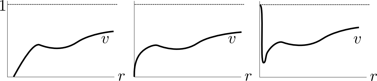
Figure 4. An illustration of the function vv in terms of rr before, at, and after the singular time. We do not use exact numerics but do pay attention to asymptotics at r=0r=0.

2. Existence

In this section we prove the existence theorem, Theorem 4, except for the construction of barriers which is done in Section 4. Sections 2.1 and 2.2 prove things about the evolution near the singular point. These Sections are purely on the level of looking at a parabolic PDE on an interval. In Sections 2.3, 2.4, and 2.5 we construct a forward evolution as a limit of forward evolutions from smooth initial metrics. A small amount of work is need to glue the results about regularity near the singular point to regularity results for Ricci flow in the smooth region.

2.1. Avoidance Principle and Barriers

We use the avoidance principle to trap solutions (v,hv,h) to (44), (47) in a simple “square”:

(58) {(v,h):\displaystyle\{(v,h):\; for all (r,t)∈[r1,r2]×[t1,t2]}\displaystyle\text{ for all }(r,t)\in[r_{1},r_{2}]\times[t_{1},t_{2}]\}
(59) (v⁡(r,t),h⁡(r,t))∈[v−​(r,t),v+​(r,t)]×[h−​(r,t),h+​(r,t)]\displaystyle(v(r,t),h(r,t))\in[v^{-}(r,t),v^{+}(r,t)]\times[h^{-}(r,t),h^{+}(r,t)]

In general, the term in the evolution of vv which involves derivatives of hh,

(60) −2​p​vh​ψs2=−12​v2​hr2h\displaystyle-2p\frac{v}{h}\psi_{s}^{2}=-\tfrac{1}{2}v^{2}\frac{h_{r}^{2}}{h}

could cause difficulty in using an avoidance principle; if (v,h)(v,h) is on the v=v+v=v^{+} boundary of such a set we cannot have any knowledge about hrh_{r}. In our situation, we are saved by the fact that we have the preserved gradient bound (52). Luckily, this term never dominates our calculations, so we never need fine control on it and the following ad hoc definition of barriers suffices.

Definition 8 (Barriers).

Functions v+v^{+}, v−v^{-}, h+h^{+}, h−h^{-} which are C2C^{2} on [r1,r2]×[t1,t2][r_{1},r_{2}]\times[t_{1},t_{2}] are called barriers if

  • •

    The barriers are properly ordered:

    (61) v−<v+,h−<h+.\displaystyle v^{-}<v^{+},\quad h^{-}<h^{+}.
  • •

    v±v^{\pm} are sub/supersolutions: For all h∗h^{*} with h−≤h∗h^{-}\leq h^{*} and for all u∗u^{*} with 0≤u∗≤10\leq u^{*}\leq 1 we have

    (62) ∂tv−−𝒢(v)​(v−,h∗,u∗)≤0≤∂tv+−𝒢(v)​(v+,h,u∗).\displaystyle\partial_{t}v^{-}-\mathcal{G}^{(v)}(v^{-},h^{*},u^{*})\leq 0\leq\partial_{t}v^{+}-\mathcal{G}^{(v)}(v^{+},h,u^{*}).
  • •

    h±h^{\pm} are sub/supersolutions: For all v∗v^{*} with v−≤v∗≤v+v^{-}\leq v^{*}\leq v^{+} and for all u∗u^{*} with 0≤u∗≤10\leq u^{*}\leq 1 we have

    (63) ∂th−−𝒢(h)​(v∗,h−,u∗)≤0≤∂th+−𝒢(h)​(v∗,h+,u∗).\displaystyle\partial_{t}h^{-}-\mathcal{G}^{(h)}(v^{*},h^{-},u^{*})\leq 0\leq\partial_{t}h^{+}-\mathcal{G}^{(h)}(v^{*},h^{+},u^{*}).
  • •

    Smoothness conditions at zero: If r1=0r_{1}=0 then

    (64) v−​(0,t)=v+​(0,t)=1,∂rv−​(0,t)=∂rv+​(0,t)=0,\displaystyle v^{-}(0,t)=v^{+}(0,t)=1,\quad\partial_{r}v^{-}(0,t)=\partial_{r}v^{+}(0,t)=0,
    (65) 0<h−​(0,t)<h+​(0,t),∂rh−​(0,t)=∂rh+​(0,t)=0.\displaystyle 0<h^{-}(0,t)<h^{+}(0,t),\quad\partial_{r}h^{-}(0,t)=\partial_{r}h^{+}(0,t)=0.

Our equations will have Neumann boundary conditions at r=0r=0, and we may think of r=0r=0 as an interior point. Therefore we use the following definition of parabolic boundary.

Definition 9.

The parabolic boundary of [r1,r2]×[t1,t2][r_{1},r_{2}]\times[t_{1},t_{2}] is defined to be

(66) ([r1,r2]×{t1})∪({r1}×[t1,t2])∪({r2}×[t1,t2])\displaystyle\left([r_{1},r_{2}]\times\{t_{1}\}\right)\cup\left(\{r_{1}\}\times[t_{1},t_{2}]\right)\cup\left(\{r_{2}\}\times[t_{1},t_{2}]\right)

if r1>0r_{1}>0 or

(67) ([0,r2]×{t1})∪({r2}×[t1,t2])\displaystyle\left([0,r_{2}]\times\{t_{1}\}\right)\cup\left(\{r_{2}\}\times[t_{1},t_{2}]\right)

if r1=0r_{1}=0.

For our barriers, we have the following avoidance principle. We state it with a slight contrapositive compared to the usual statement; we say “if a solution crosses the barriers, it crosses on the parabolic boundary first”.

Lemma 10.

Suppose that v+v^{+}, v−v^{-}, h+h^{+}, h−h^{-} are barriers on [r1,r2]×[t1,t2][r_{1},r_{2}]\times[t_{1},t_{2}], vv and hh evolve by (57) and hh satisfies the gradient bound (52). Define L−=r−2​(1−v−)L^{-}=r^{-2}(1-v^{-}), L=r−2​(1−v)L=r^{-2}(1-v), L+=r−2​(1−v+)L^{+}=r^{-2}(1-v^{+}). If r1=0r_{1}=0 then suppose these functions are defined at r=0r=0 by their limit as r↘0r\searrow 0 and that L−,L,L+,h−,h,h+L^{-},L,L^{+},h^{-},h,h^{+} satisfy the Neumann condition ∂r(⋅)=0\partial_{r}(\cdot)=0 at r=0r=0.

Let t0t_{0} be the infimum of the times for which one of the inequalities

(68) −L−<−L<−L+,h−<h<h+,.\displaystyle-L^{-}<-L<-L^{+},\quad h^{-}<h<h^{+},.

is violated. Then there is an r0r_{0} so that one of the inequalities (68) is violated at (r0,t0)(r_{0},t_{0}) and (r0,t0)(r_{0},t_{0}) is on the parabolic boundary of [r1,t1][r_{1},t_{1}].

Proof.

The case r1>0r_{1}>0 is a standard basic comparison principle argument.

To deal with the case r1=0r_{1}=0, note that using the Neumann condition, the equation for both LL and hh allows for comparison at r=0r=0. (Essentially this is because r=0r=0 is secretly an interior point of the symmetric manifold.) ∎

We will apply the above lemma where r1r_{1} and r2r_{2} depend on tt, or r1≡0r_{1}\equiv 0. The proof is the same. We will also need to glue barriers which are defined in different space-time regions.

Definition 11 (Gluing Conditions).

Suppose (v^−,v^+,h^−,h^+)(\hat{v}^{-},\hat{v}^{+},\hat{h}^{-},\hat{h}^{+}) are barriers are [r^1,r^2]×[t1,t2][\hat{r}_{1},\hat{r}_{2}]\times[t_{1},t_{2}] and (v~−,v~+,h~−,h~+)(\tilde{v}^{-},\tilde{v}^{+},\tilde{h}^{-},\tilde{h}^{+}) are barriers on [r~1,r~2]×[t1,t2][\tilde{r}_{1},\tilde{r}_{2}]\times[t_{1},t_{2}]. We say these satisfy the gluing conditions if r^1<r~1<r^2<r~2\hat{r}_{1}<\tilde{r}_{1}<\hat{r}_{2}<\tilde{r}_{2} and

(69) v^−​(r~1,t)>v~−​(r~1,t),v~−​(r2,t)>v^−​(r2,t),\displaystyle\hat{v}^{-}(\tilde{r}_{1},t)>\tilde{v}^{-}(\tilde{r}_{1},t),\quad\tilde{v}^{-}(r_{2},t)>\hat{v}^{-}(r_{2},t),
(70) v^+​(r~1,t)<v~+​(r~1,t),v~+​(r2,t)<v^+​(r2,t).\displaystyle\hat{v}^{+}(\tilde{r}_{1},t)<\tilde{v}^{+}(\tilde{r}_{1},t),\quad\tilde{v}^{+}(r_{2},t)<\hat{v}^{+}(r_{2},t).

And similarly for h^−,h^+,h~−,h~+\hat{h}^{-},\hat{h}^{+},\tilde{h}^{-},\tilde{h}^{+}.

If two sets of barriers satisfy the gluing conditions, then we can conclude that a solution is trapped between both on [r^1,r~2]×[t1,t2][\hat{r}_{1},\tilde{r}_{2}]\times[t_{1},t_{2}] if we only check the boundary conditions on the parabolic boundary of [r^1,r~2]×[t1,t2][\hat{r}_{1},\tilde{r}_{2}]\times[t_{1},t_{2}]. One way to see this is to go to the proof of Lemma 10 and check that a solution cannot touch max⁡(v^−,v~−)\max(\hat{v}^{-},\tilde{v}^{-}) from above at a point where it transitions from v−v^{-} to v~−\tilde{v}^{-}. Perhaps a cleaner way is to just use Lemma 10 twice. Applied to the hat barriers it says a solution has to have its first crossing of the hat barriers on the parabolic boundary of [r^1,r^2]×[t1,t2][\hat{r}_{1},\hat{r}_{2}]\times[t_{1},t_{2}]. But if it crosses at r=r^2r=\hat{r}_{2} first, then by the gluing conditions it has crossed the tilde barriers at r^2∈[r~1,r~2]\hat{r}_{2}\in[\tilde{r}_{1},\tilde{r}_{2}] before r~1\tilde{r}_{1}, so by Lemma 10 it must have crossed the tilde barriers at r~2\tilde{r}_{2} first.

Region Barrier for vv Barrier for hh
Outer a±2​(1+(1±ϵ)​αq2​t​r−2)​v0a^{2}_{\pm}(1+(1\pm\epsilon)\alpha_{q}^{2}tr^{-2})v_{0} b±2​(1+(1±ϵ)​αq2​t​r−2)​h0b^{2}_{\pm}(1+(1\pm\epsilon)\alpha_{q}^{2}tr^{-2})h_{0}
Parabolic 2​a^±2​(1+αq2​(1±D​|τ|−1​ρ−2)​ρ−2)2\hat{a}^{2}_{\pm}(1+\alpha_{q}^{2}(1\pm D|\tau|^{-1}\rho^{-2})\rho^{-2}) 12​b^±2​(ρ2+αq2​(1±D​|τ|−1​ρ−2))\tfrac{1}{2}\hat{b}^{2}_{\pm}(\rho^{2}+\alpha_{q}^{2}(1\pm D|\tau|^{-1}\rho^{-2}))
Tip ℬ⁡(c±​ζ)+(1∓ϵ)​|τ|−1​c±−2​𝒞​(c±​ζ)\mathcal{B}(c_{\pm}\zeta)+(1\mp\epsilon)|\tau|^{-1}c^{-2}_{\pm}\mathcal{C}(c_{\pm}\zeta) αq4​c¯±2+|τ|−1​𝒜​(c±​ζ)\alpha_{q}^{4}\bar{c}_{\pm}^{2}+|\tau|^{-1}\mathcal{A}(c_{\pm}\zeta)
Table 1. The barriers used in each region described in Lemma 12

The construction of barriers is conceptually simple, but it introduces a number of unsightly constants and has been relegated to Section 4. The reader who wishes to know where the asymptotics of the forward evolution come from may read the formal asymptotics in Section 3. The result of the lemmas of Section 4 is the following.

Lemma 12.

Let δ,ϵ>0\delta,\epsilon>0 be given and uniformly small. Then there is r∗>0r_{*}>0 and t∗>0t_{*}>0 so that [0,r∗]×(0,T∗][0,r_{*}]\times(0,T_{*}], is covered by three sets of barriers. Specifically, there are constants C1,C2C_{1},C_{2} independent of ϵ,δ\epsilon,\delta so that

  • •

    Let ρ=r/t\rho=r/\sqrt{t}. In the outer region given by,

    {ρ≥C1/ϵ and r<r∗}=:{(r,t):tϵC1<r<r∗},\{\rho\geq C_{1}/\sqrt{\epsilon}\text{ and }r<r_{*}\}=\vcentcolon\{(r,t):\sqrt{\frac{t}{\epsilon}}C_{1}<r<r_{*}\},

    the barriers are the outer region barriers in Table 1, detailed in Lemma 23.

  • •

    Let ζ=|log⁡t|​ρ\zeta=|\log t|\rho. In the parabolic region given by,

    {ρ<2C1/ϵ and ζ>C2/ϵ}=:{(r,t):tϵ​|log⁡t|C2<r<tϵ2C1},\{\rho<2C_{1}/\sqrt{\epsilon}\text{ and }\zeta>C_{2}/\sqrt{\epsilon}\}=\vcentcolon\left\{(r,t):\sqrt{\frac{t}{\epsilon|\log t|}}C_{2}<r<\sqrt{\frac{t}{\epsilon}}2C_{1}\right\},

    the barriers are the parabolic region barriers in Table 1, detailed in Lemma 24, with constants

    (71) a^±2=k2+o⁡(|ϵ|+|δ|),b^±2=k−2+o⁡(|ϵ|+|δ|)\displaystyle\hat{a}^{2}_{\pm}=k^{2}+o\left(|\epsilon|+|\delta|\right),\quad\hat{b}^{2}_{\pm}=k^{-2}+o\left(|\epsilon|+|\delta|\right)
  • •

    In the tip region given by,

    {ζ<2C2/ϵ}=:{(r,t):r<tϵ​|log⁡t|2C2}\{\zeta<2C_{2}/\sqrt{\epsilon}\}=\vcentcolon\left\{(r,t):r<\sqrt{\frac{t}{\epsilon|\log t|}}2C_{2}\right\}

    the barriers are the tip region barriers in Table 1, detailed in Lemma 25, with constants

    (72) c¯±=c0+o⁡(|ϵ|+|δ|),c±=c0+o⁡(|ϵ|+|δ|)\displaystyle\bar{c}_{\pm}=c_{0}+o(|\epsilon|+|\delta|),\quad c_{\pm}=c_{0}+o(|\epsilon|+|\delta|)
  • •

    The gluing conditions are satisfied between the outer and parabolic region barriers, and between the parabolic and tip region barriers.

By design the outer barriers contain the initial data. Therefore by the first point, any metric with the asymptotics (5) will be contained by the barriers at time zero, in a smaller region [0,r∗][0,r_{*}]. Also, any functions between the barriers for positive time will satisfy the assumptions for Lemma 13 below. This is because the barriers in the tip region trap vv in the correct manner near r=0r=0. We will not (and cannot) directly apply Lemma 10 to the barriers on [0,T∗][0,T_{*}], but we will apply it on [t1,T∗][t_{1},T_{*}].

2.2. Parabolic Regularity

In this section we apply regularity results for parabolic partial differential equations to our situation. We prove two lemmas which will allow us to get regularity for solutions provided vv and hh stay in bounded regions.

Lemma 13.

Let v≥0v\geq 0 and h≥0h\geq 0 satisfy (44), (47) on [0,r2]×[t1,t2)[0,r_{2}]\times[t_{1},t_{2}), with

(73) ∂rv⁡(0,t)=∂rh⁡(0,t)=0.\displaystyle\partial_{r}v(0,t)=\partial_{r}h(0,t)=0.

Suppose the gradient bounds (50) and (52) are satisfied. Let f=1−vr2=1−ϕsϕ2f=\frac{1-\sqrt{v}}{r^{2}}=\frac{1-\phi_{s}}{\phi^{2}}. Suppose

(74) sup[0,r2]×[t1,t2)f<C1,sup[0,r2]×[t1,t2)h<C1,\displaystyle\sup_{[0,r_{2}]\times[t_{1},t_{2})}f<C_{1},\qquad\sup_{[0,r_{2}]\times[t_{1},t_{2})}h<C_{1},
(75) inf[0,r2]×[t1,t2)v>C1−1,inf[0,r2]×[t1,t2)h>C1−1,\displaystyle\inf_{[0,r_{2}]\times[t_{1},t_{2})}v>C_{1}^{-1},\qquad\inf_{[0,r_{2}]\times[t_{1},t_{2})}h>C_{1}^{-1},

and let t1′>t1t_{1}^{\prime}>t_{1} and r2′<r2r_{2}^{\prime}<r_{2} be given.

Then there is C2<∞C_{2}<\infty depending on C,r2,r2′,t1,t1′,t2,p,qC,r_{2},r_{2}^{\prime},t_{1},t_{1}^{\prime},t_{2},p,q such that

(76) sup[0,r2′]×[t1′,t2)|Rm|<C2\displaystyle\sup_{[0,r_{2}^{\prime}]\times[t_{1}^{\prime},t_{2})}|\Rm|<C_{2}

where Rm\Rm is the curvature of the associated doubly warped product metric.

Proof.

The sectional curvatures are smooth functions of hh, hrh_{r}, hr​rh_{rr}, and ff, frf_{r}, so it suffices to control those.

The function ff satisfies

(77) ft\displaystyle f_{t} =[1−2​f​r2+f2​r4]​fr​r\displaystyle=\left[1-2fr^{2}+f^{2}r^{4}\right]f_{rr}
(78) +q+2r​fr+[3​r3​f2−6​r​f]​fr\displaystyle+\frac{q+2}{r}f_{r}+\left[3r^{3}f^{2}-6rf\right]f_{r}
(79) +[−r2​q​f+r2​f+3​q−3−p2​1h​v​hr2h]​f2\displaystyle+\left[-r^{2}qf+r^{2}f+3q-3-\frac{p}{2}\frac{1}{h}\frac{vh_{r}^{2}}{h}\right]f^{2}

Think of ff as a rotationally symmetric function in B(0,r2)⊂q+3B(0,r_{2})\subset\real^{q+3}. Then by our assumptions the equation (79) is a uniformly parabolic equation with coefficients which depend on space and time but have an L∞L^{\infty} bound. By the De Giorgi-Nash-Moser theorem (Theorem 6.28 in [Lie96] works here) ff is in the Hölder space Cα​(B⁡(0,r2′)×[t1′,t2))C^{\alpha}(B(0,r_{2}^{\prime})\times[t_{1}^{\prime},t_{2})) with α\alpha and the CαC^{\alpha} norm only depending on the allowed numbers.

We know already that hh is uniformly in C1C^{1}, because we assumed the gradient bound hr2≤hvh_{r}^{2}\leq\frac{h}{v}. Now that we know vv is uniformly Hölder, the coefficients in the evolution for hh are uniformly Hölder. We can multiply by a cut-off function to get a solution to an inhomogeneous equation with zero boundary data. Then the Schauder estimate gives a uniform bound on |hr​r||h_{rr}|. Theorem 3 of [Sch94] has a clean statement of the Schauder estimate in a more general case than we need here. (At the moment we are not actually applying the Schauder estimate to a system, only to the equation for hh.)

Once we have the uniform bound on |hr​r||h_{rr}| we get that the coefficients in the evolution of ff are Hölder, so applying the Schauder estimate gives a C2C^{2} bound on ff. ∎

Outside of the region where r=0r=0, the relevant functions satisfy nice parabolic equations in one dimension, and we can actually get regularity up to the starting time t=0t=0.

Lemma 14.

Let vv and hh be as in the hypotheses of Lemma 13, but instead defined on [r1,r2]×[0,t2)[r_{1},r_{2}]\times[0,t_{2}) with r1>0r_{1}>0. Suppose also that at t=0t=0 both have H1​([r1,r2])H^{1}([r_{1},r_{2}]) bounds:

(80) ∫r1r2(∂rv⁡(r,0))2​𝑑r<C1,∫r1r2(∂rh⁡(r,0))2​𝑑r<C1.\displaystyle\int_{r_{1}}^{r_{2}}(\partial_{r}v(r,0))^{2}dr<C_{1},\qquad\int_{r_{1}}^{r_{2}}(\partial_{r}h(r,0))^{2}dr<C_{1}.

Let r1′r_{1}^{\prime} and r2′r_{2}^{\prime} be given with r1<r1′<r2′<r2r_{1}<r_{1}^{\prime}<r_{2}^{\prime}<r_{2}. There is a C2C_{2} depending on C1,r1,r1′,r2,r2′,p,qC_{1},r_{1},r_{1}^{\prime},r_{2},r_{2}^{\prime},p,q so that

(81) sup[r1′,r2′]×[0,t2)|Rm|<C2\displaystyle\sup_{[r_{1}^{\prime},r_{2}^{\prime}]\times[0,t_{2})}|\Rm|<C_{2}
Proof.

Taking η\eta to be a static smooth cut-off function, v⋅ηv\cdot\eta satisfies a parabolic equation on [r1,r2][r_{1},r_{2}] with zero boundary data, bounded coefficients and bounded right hand side. (In particular, the terms involving 1/r1/r are bounded because r1>0r_{1}>0). Therefore for all tt the solution is uniformly in H1​([r1,r2])H^{1}([r_{1},r_{2}]) (Theorem 6.1 of [Lie96]). The Sobolev embedding in one dimension tells us that vv is in CαC^{\alpha} for α≤1/2\alpha\leq 1/2. Then as in the proof of Lemma 13, the conclusion follows from the Schauder estimate. ∎

2.3. Mollified flows

We create smooth initial metrics which approximate our singular metric gi​n​i​tg_{init}.

Definition 15.

Let gi​n​i​tg_{init} be given satisfying the assumptions of Theorem 4. Let {gω}ω∈(0,ω∗)\{g_{\omega}\}_{\omega\in(0,\omega_{*})} be a one parameter family of smooth metrics on MM such that

  • •

    Mr>ωM_{r>\sqrt{\omega}} is identical for gi​n​i​tg_{init} and gωg_{\omega}, and the metrics agree there.

  • •

    gωg_{\omega} is a smooth metric and satisfies the gradient bound (4).

  • •

    For some fixed r#r_{\#}, ϕω\phi_{\omega} is increasing for r<r#r<r_{\#}, so the rr coordinate is defined on Nr<r#N_{r<r_{\#}}. (Recall Definition 3 for the notation Nr<r#N_{r<r_{\#}}.) In terms of these coordinates, hω​(0)h_{\omega}(0) and vω​(0)v_{\omega}(0) lie between barriers from Theorem 12, evaluated at a small positive time. In particular, take the barriers for any small ϵ\epsilon and δ\delta, and evaluate them at time

    tω=ϵC3​ωt_{\omega}=\frac{\epsilon}{\sqrt{C_{3}}}\omega

    for a sufficiently large C3C_{3}.

We take tω≲ωt_{\omega}\lesssim\omega above because we need very little time to pass, so that the barriers still trap the initial function at r=ωr=\sqrt{\omega}. In particular (r,t)=(ω,tω)(r,t)=(\sqrt{\omega},t_{\omega}) is in the outer region.

Each gωg_{\omega} has sup|Rm|<Cω\sup|\Rm|<C_{\omega}. Shi’s short time existence theorem [Shi89] gives us a Ricci flow starting from gωg_{\omega} on some time interval [0,Tω)[0,T_{\omega}). (We must turn to [Shi89] here because we allow for noncompact initial data.) We wish to show first that in fact Tω≥T0>0T_{\omega}\geq T_{0}>0. Then, we want bounds on curvatures away from the singularity. This allows us to get convergence of a subsequence gωkg_{\omega_{k}} to a solution to Ricci flow emerging from the initial metric.

In principle the existence time and regularity works because the relevant functions will satisfy partial differential equations similar to

(82) ∂tu⁡(x,t)=∂x(a⁡(u)​∂xu)+b⁡(u)​∂xu+c⁡(u)​u\displaystyle\partial_{t}u(x,t)=\partial_{x}(a(u)\partial_{x}u)+b(u)\partial_{x}u+c(u)u

whose solutions are great as long as the coefficients a⁡(u)a(u), b⁡(u)b(u) and c⁡(u)c(u) do not do anything bad. The barriers will tell us that the coefficients behave reasonably. There is some extra work because our barriers are not defined on the whole of the manifold MM, and so the solution might cross the barriers on the edge of the domain where they are defined (where r=r∗r=r_{*}). This problem is overcome in Lemmas 17 and 18 because on the complement of the region where the barriers are defined, the initial metrics are uniformly smooth (and in fact identical).

2.4. Outer Control

Let us define Tω†T^{\dagger}_{\omega} to be the first time that one of the following fails (or Tω†=TωT^{\dagger}_{\omega}=T_{\omega} if the metric becomes singular before on of the following happen):

  1. (1)

    The function ϕω\phi_{\omega} is not strictly increasing (from the tip) until ϕω=r∗\phi_{\omega}=r_{*}, and therefore the rr coordinate is defined up to r=r∗r=r_{*}.

  2. (2)

    The functions vω​(r,t)v_{\omega}(r,t) and hω​(r,t)h_{\omega}(r,t) do not cross the time-shifted barriers at r=r∗r=r_{*}.

Thus on the interval [0,Tω†)[0,T^{\dagger}_{\omega}) both of the above hold for the metric gωg_{\omega}. Both (1) and (2) both hold for a small time (because they hold for gω​(0)g_{\omega}(0) and the functions vω=(∂sϕω)2v_{\omega}=(\partial_{s}\phi_{\omega})^{2} and h=ψω2h=\psi_{\omega}^{2} are continuous in time). Also (1) cannot fail before vω↘0v_{\omega}\searrow 0 for some r<r∗r<r_{*}. Since vω±​(r,t)>0v_{\omega}^{\pm}(r,t)>0, the avoidance principle implies that while (2) holds, (1) will hold. So Tω†T^{\dagger}_{\omega} can actually be characterized as the first time when (2) fails.

We want to show that Tω†=min⁡(Tω,T0)T^{\dagger}_{\omega}=\min(T_{\omega},T_{0}) for T0T_{0} independent of ω\omega. We do this in Lemmas 16 to 18. If MM is compact then an alternative way to get the |Rm||\Rm| bounds in Lemmas 16 and 17 would be to use pseudolocality theorem (Theorem 10.3 of [Per02]). As the metrics gω​(0)g_{\omega}(0) all agree on Mr>r∗M_{r>r_{*}} they will satisfy uniform curvature and volume bounds on a small enough scale, so there is a uniform curvature bound on a smaller scale as long as the Ricci flow exists. This was the method used in [GS16].

There is a technicality in the following discussion. The set Nr<r∗N_{r<r_{*}} (defined in Definition 3) depends on time and ω\omega, but we can think of vv and hh as defined on the fixed box [0,r∗]×[0,Tω†][0,r_{*}]\times[0,T^{\dagger}_{\omega}].

Lemma 16.

Consider the metrics gωg_{\omega}, which have the rr coordinate defined on Nr<r∗N_{r<r_{*}} and are trapped between the barriers on [0,r∗]×[0,Tω†)[0,r_{*}]\times[0,T^{\dagger}_{\omega}).

Then for some time we have curvature bounds in a smaller region. Precisely, there is a T0T_{0} so that

(83) supt∈[0,min⁡(Tω†,T0)]supp∈N12​r∗<r<34​r∗|Rmgω​(t)|(p)<C0\displaystyle\sup_{t\in[0,\min(T^{\dagger}_{\omega},T_{0})]}\quad\sup_{p\in N_{\frac{1}{2}r_{*}<r<\frac{3}{4}r_{*}}}|\Rm_{g_{\omega}(t)}|(p)<C_{0}

for some C0C_{0} independent of ω\omega.

Proof.

As long as the metric coefficients are trapped between the barriers, they satisfy the hypotheses of Lemma 14 on the interval [14​r∗,r∗]\left[\frac{1}{4}r_{*},r_{*}\right], which uses results for parabolic PDE in one dimension to control |Rm||\Rm| on the smaller interval [12​r∗,34​r∗][\frac{1}{2}r_{*},\frac{3}{4}r_{*}]. ∎

The uniform bound on |Rm||\Rm| in the strip Na​r∗<r<b​r∗N_{ar_{*}<r<br_{*}} lets us get a uniform bound on |Rm||\Rm| away from M−Nr<a​r∗=Mr>a​r∗M-N_{r<ar_{*}}=M_{r>ar_{*}}.

Lemma 17.

There is a T0T_{0} and C0C_{0} independent of ω\omega such that for t∈[0,min⁡(T0,Tω†)]t\in[0,\min(T_{0},T^{\dagger}_{\omega})] and p∈Mr>a​r∗p\in M_{r>ar_{*}} we have

(84) |Rmgω​(t)|​(p)<C0.\displaystyle|\Rm_{g_{\omega}(t)}|(p)<C_{0}.

Also, there are constants CkC_{k} for k∈ℕk\in\mathbb{N} so that for points pp in the smaller region Mr>b​r∗M_{r>br_{*}} we have

(85) |∇kRmgω​(t)|​(p)<Ck\displaystyle|\nabla^{k}\Rm_{g_{\omega}(t)}|(p)<C_{k}
Proof.

On Mr>a​r∗M_{r>ar_{*}}, |Rm||\Rm| is uniformly bounded at the initial time. Under Ricci flow |Rm||\Rm| satisfies

(86) ∂t|Rm|2≤Δ​|Rm|2+c​(|Rm|2)3/2.\displaystyle\partial_{t}|\Rm|^{2}\leq\Delta|\Rm|^{2}+c(|\Rm|^{2})^{3/2}.

Here cc depends only on the dimension of the space. Lemma 16 tells us that |Rm||\Rm| is bounded near the boundary of Mr>a​r∗M_{r>ar_{*}}. The first part of the theorem follows from the maximum principle.

To get the control on the derivatives, we use the local Shi’s estimates given in 14.4.1 of [CCG+07]. These control derivatives on a fixed compact set KK, whereas Mr≥r∗M_{r\geq r_{*}} is changing in time; this is the technicality mentioned earlier. This problem is easily overcome because we have bounds on |Rm||\Rm| and hence on ∂tgω\partial_{t}g_{\omega}. This implies that the time-dependent set Nr>b​r∗​[gω​(t)]N_{r>br_{*}}[g_{\omega}(t)] is contained in the fixed set Nr>a​r∗​[gω​(0)]N_{r>ar_{*}}[g_{\omega}(0)] for small time. We apply the local Shi estimates on this fixed compact set. ∎

Lemma 18.

There is a T0T_{0} independent of ω\omega so that Tω†≥min⁡(T0,Tω)T^{\dagger}_{\omega}\geq\min(T_{0},T_{\omega}).

Proof.

Lemma 17 gives us a uniform bound on |Rm||\Rm| and its derivatives on Mr>b​r∗M_{r>br_{*}}, which implies that in a small time interval the metric and its derivatives, in some fixed coordinate system, can only change so much there. In particular we can write gω​(t)g_{\omega}(t) near r∗r_{*} as

(87) gω​(t)\displaystyle g_{\omega}(t) =(1vi​n​i​t​(r,0)+α⁡(r,t))​d​r2\displaystyle=\left(\frac{1}{v_{init}(r,0)}+\alpha(r,t)\right)dr^{2}
(88) +(hi​n​i​t​(r,0)+β⁡(r,t))​gSp+(r2+γ⁡(r,t))​gSq,\displaystyle+(h_{init}(r,0)+\beta(r,t))g_{S^{p}}+(r^{2}+\gamma(r,t))g_{S^{q}},

with rr signifying a fixed coordinate, and where α\alpha, β\beta, and γ\gamma ae zero at t=0t=0. By Lemma 17, for small time α\alpha, β\beta, and γ\gamma will be small with small derivatives, independently of ω\omega. At r=r∗r=r_{*}, the functions v⁡(r,t)v(r,t) and h⁡(r,t)h(r,t) depend in smooth ways on α\alpha, β\beta, and γ\gamma. By choosing T0T_{0} small enough, vv and hh will not have enough time to cross the barriers. ∎

2.5. Uniform curvature bounds and convergence

Lemma 19.

There is T0T_{0} independent of ω\omega such that Tω≥T0T_{\omega}\geq T_{0}.

Proof.

Ricci flow exists up to a time when |Rm||\Rm| goes to infinity. First, suppose TωT_{\omega} is smaller than the time when the functions vv and hh are trapped between barriers, and we will bound |Rm||\Rm|. Here we are not worried about a uniform with respect to ω\omega, only about getting some bound if TωT_{\omega} is small.

By Lemma 18, the metric coefficients do not cross the barriers at r=r∗r=r_{*}, so by the avoidance principle they are trapped between the barriers on Nr<r∗N_{r<r_{*}}. If TωT_{\omega} is smaller than the time when the coefficients are trapped, then we can bound |Rm||\Rm| by using Lemma 13 in Nr<r∗N_{r<r_{*}}, Lemma 14 in Na​r∗<r<b​r∗N_{ar_{*}<r<br_{*}}, and Lemma 17 in Mr>a​r∗M_{r>ar_{*}}. ∎

Lemma 20.

There is a T0T_{0} independent of ω\omega so that we have the following curvature bounds for t<T0t<T_{0}.

For any r1>0r_{1}>0 and k∈ℕ∪{0}k\in\mathbb{N}\cup\{0\} there is Ck​(r1)<∞C_{k}(r_{1})<\infty such that

(89) supt∈[0,T0]supp∈Mr>r1|∇kRmgω​(t)|​(p)<Ck​(r1).\displaystyle\sup_{t\in[0,T_{0}]}\quad\sup_{p\in M_{r>r_{1}}}|\nabla^{k}\Rm_{g_{\omega}(t)}|(p)<C_{k}(r_{1}).

For any t1>0t_{1}>0 and k∈ℕ∪{0}k\in\mathbb{N}\cup\{0\} there is C~k​(t1)<∞\tilde{C}_{k}(t_{1})<\infty such that

(90) supt∈[t1,T0]supp∈M|Rmgω​(t)|​(p)<C~k​(t1)\displaystyle\sup_{t\in[t_{1},T_{0}]}\quad\sup_{p\in M}|\Rm_{g_{\omega}(t)}|(p)<\tilde{C}_{k}(t_{1})
Proof.

The bounds for r>r1r>r_{1} follow the same path as the bounds for r>r∗r>r_{*} in Section 2.4. Briefly: bounds on |Rm||\Rm| in [(1/2)​r1,(3/4)​r1][(1/2)r_{1},(3/4)r_{1}] follow from the parabolic regularity in Lemma 16, then bounds on Mr>r1M_{r>r_{1}} follow by the maximum principle and Shi’s estimates as in Lemma 17.

Now we explain the bounds for t>t1t>t_{1}. When t≥t1/2t\geq t_{1}/2 the functions vω​(t)v_{\omega}(t) and hω​(t)h_{\omega}(t) are between the barriers evaluated at time t≥t1/2+ω≥t1/2t\geq t_{1}/2+\omega\geq t_{1}/2. For positive time the barriers force the functions to behave well, i.e. vωv_{\omega} and hωh_{\omega} satisfy the bounds required in Lemma 13. Therefore we have |Rm||\Rm| bounds for t≥(3/4)​t1t\geq(3/4)t_{1} (in Nr<r∗N_{r<r_{*}} by Lemma 13 and outside of Nr<r∗N_{r<r_{*}} by the previous paragraph) and then Shi’s global estimates [Shi89] imply bounds on derivatives of curvature for t≥t1t\geq t_{1}. ∎

Lemma 21.

A subsequence of the mollified solutions gωg_{\omega} converge to a solution g∗g_{*} of Ricci flow on Cl​o​c∞​(M×[0,T0]−Ns=0×{0})C^{\infty}_{loc}(M\times[0,T_{0}]-N_{s=0}\times\{0\}). The solution g∗g_{*} agrees with gi​n​i​tg_{init} at t=0t=0 and is smooth for t>0t>0.

Proof.

This Lemma follows from compactness, and the previous lemmata which tell us that the solutions are reasonable enough. There are a couple of technicalities which come up from having to choose coordinates. The full proof is the same as in Theorem 5.10 of [Car16] or Lemmas 12 and 13 of [ACK12]. ∎

3. Formal Calculations

3.1. Formal solution in the outer region

As an initial approximation to the forward evolution, we may use

vo​u​t\displaystyle v_{out} ≈v0+t​ℱ(v)​(v0,h0),\displaystyle\approx v_{0}+t\mathcal{F}^{(v)}(v_{0},h_{0}),
ho​u​t\displaystyle h_{out} ≈h0+t​ℱ(h)​(v0,h0).\displaystyle\approx h_{0}+t\mathcal{F}^{(h)}(v_{0},h_{0}).

We calculate some derivatives of v0v_{0} and h0h_{0}. All these calculations use the simple fact that as r↘0r\searrow 0,

(91) ∂r(rp​|log⁡r|q)=(1+o⁡(1))⋅{p​rp−1​|log⁡r|qp≠0−q​rp−1​|log⁡r|q−1p=0\displaystyle\partial_{r}\left(r^{p}|\log r|^{q}\right)=(1+o(1))\cdot\begin{cases}pr^{p-1}|\log r|^{q}&p\neq 0\\ -qr^{p-1}|\log r|^{q-1}&p=0\end{cases}
v0\displaystyle v_{0} =k2​|log⁡r|−1\displaystyle=k^{2}|\log r|^{-1} h0\displaystyle h_{0} =1k2​r2​|log⁡r|\displaystyle=\frac{1}{k^{2}}r^{2}|\log r|
v0,r\displaystyle v_{0,r} =k2​r−1​|log⁡r|−2\displaystyle=k^{2}r^{-1}|\log r|^{-2} h0,r\displaystyle h_{0,r} =1k2​2​r​|log⁡r|​(1+o⁡(1))\displaystyle=\frac{1}{k^{2}}2r|\log r|(1+o(1))
v0,r​r\displaystyle v_{0,rr} =−k2​r−2​|log⁡r|−2​(1+o⁡(1))\displaystyle=-k^{2}r^{-2}|\log r|^{-2}(1+o(1)) h0,r​r\displaystyle h_{0,rr} =1k2​2​|log⁡r|​(1+o⁡(1))\displaystyle=\frac{1}{k^{2}}2|\log r|(1+o(1))

Now calculate ℱ(v)​[v0,h0]\mathcal{F}^{(v)}[v_{0},h_{0}] and ℱ(h)​[v0,h0]\mathcal{F}^{(h)}[v_{0},h_{0}]. First, the leading term in

ℱ(v)​[v,h]=v​vr​r−12​vr2−r−1​v​vr+αq2​r−2​v​(1−v)+12​αq2​r−1​vr−12​p​vh​(v​hr2h)\displaystyle\mathcal{F}^{(v)}[v,h]=vv_{rr}-\tfrac{1}{2}v_{r}^{2}-r^{-1}vv_{r}+\alpha_{q}^{2}r^{-2}v(1-v)+\tfrac{1}{2}\alpha_{q}^{2}r^{-1}v_{r}-\tfrac{1}{2}p\frac{v}{h}\left(v\frac{h_{r}^{2}}{h}\right)

is

(92) αq2​r−2​v=αq2​k2​r−2​|log⁡r|−1=αq2​r−2​v0​(r).\displaystyle\alpha_{q}^{2}r^{-2}v=\alpha_{q}^{2}k^{2}r^{-2}|\log r|^{-1}=\alpha_{q}^{2}r^{-2}v_{0}(r).

All other terms are O⁡(r−2​|log⁡r|−2)O(r^{-2}|\log r|^{-2}) or smaller.

The leading term in

ℱ(h)\displaystyle\mathcal{F}^{(h)} =v​hr​r−v​hr2h+r−1​(q−1)​hr+r−1​v​hr−2​(p−1)\displaystyle=vh_{rr}-v\frac{h_{r}^{2}}{h}+r^{-1}(q-1)h_{r}+r^{-1}vh_{r}-2(p-1)

is

(93) 12​αq2​r−1​hr=1k2​(q−1)​2​log⁡r=αq2​r−2​h0​(r).\displaystyle\tfrac{1}{2}\alpha_{q}^{2}r^{-1}h_{r}=\frac{1}{k^{2}}(q-1)2\log r=\alpha_{q}^{2}r^{-2}h_{0}(r).

All other terms are O⁡(1)O(1) or smaller.

Therefore, we take our initial approximation to be,

vo​u​t\displaystyle v_{out} =k2​1−log⁡r+t​2​(q−1)​k2​1r2​(−log⁡r)\displaystyle=k^{2}\frac{1}{-\log r}+t2(q-1)k^{2}\frac{1}{r^{2}(-\log r)}
(94) =vi​n​i​t​(1+αq2​t​r−2)\displaystyle=v_{init}(1+\alpha_{q}^{2}tr^{-2})
(95)
ho​u​t\displaystyle h_{out} =1k2​r2​(−log⁡r)+t​1k2​(q−1)​2​log⁡r\displaystyle=\frac{1}{k^{2}}r^{2}(-\log r)+t\frac{1}{k^{2}}(q-1)2\log r
(96) =hi​n​i​t​(1+αq2​t​r−2)\displaystyle=h_{init}(1+\alpha_{q}^{2}tr^{-2})

The similarity between (94) and (96) has an explanation. The leading terms in both evolutions both come from (after tracing back coordinate changes) the reaction term in the evolution for ϕ\phi, i.e. the force of the SqS^{q} factor trying to shrink. It is not a surprise that this is the leading term; near the singular point the curvature of the SqS^{q} factor is large and larger than that of the SpS^{p} factor.

As long as t≪r2t\ll r^{2} we will be able to look at ho​u​th_{out} and vo​u​tv_{out} as small perturbations of h0h_{0} and v0v_{0}, and our calculations of ℱ(v)\mathcal{F}^{(v)} and ℱ(h)\mathcal{F}^{(h)} will still be valid. In Section 3.2 we will look at the space-time region when (r,t)(r,t) goes to (0,0)(0,0) with t∼r2t\sim r^{2}.

3.2. Formal solution in the parabolic region

Our approximation in the outer region (which was a linearization in time) depends on the time derivative of vv and hh not changing too much. The approximations vo​u​tv_{out} and ho​u​th_{out} are

(97) vo​u​t=(1+o⁡(1))​vi​n​i​t,ho​u​t=(1+o⁡(1))​hi​n​i​t\displaystyle v_{out}=(1+o(1))v_{init},\quad h_{out}=(1+o(1))h_{init}

as long as r2≪tr^{2}\ll t. We use the parabolic coordinates,

(98) τ=logt,ρ=e−τ/2r,η=e−τh.\displaystyle\tau=\log t,\quad\rho=e^{-\tau/2}r,\quad\eta=e^{-\tau}h.

to study the region r2∼tr^{2}\sim t, i.e. ρ∼1\rho\sim 1.

In these coordinates, vo​u​tv_{out} and ho​u​th_{out} are

(99) vo​u​t\displaystyle v_{out} =k2|log⁡ρ+12​τ|​(1+αq2​ρ−2),\displaystyle=\frac{k^{2}}{|\log\rho+\tfrac{1}{2}\tau|}(1+\alpha_{q}^{2}\rho^{-2}),
(100) ηo​u​t\displaystyle\eta_{out} =ρ2k2​|log⁡ρ+12​τ|​(1+αq2​ρ−2)\displaystyle=\frac{\rho^{2}}{k^{2}}|\log\rho+\tfrac{1}{2}\tau|(1+\alpha_{q}^{2}\rho^{-2})
(101) =|log⁡ρ+12​τ|k2​(ρ2+αq2).\displaystyle=\frac{|\log\rho+\tfrac{1}{2}\tau|}{k^{2}}(\rho^{2}+\alpha_{q}^{2}).

So if we keep ρ\rho in a fixed region and send τ\tau to −∞-\infty,

(102) vo​u​t\displaystyle v_{out} =(1+o⁡(1))​τ−1​2​k2​(1+αq2​ρ−2),\displaystyle=(1+o(1))\tau^{-1}2k^{2}(1+\alpha_{q}^{2}\rho^{-2}),
(103) ηo​u​t\displaystyle\eta_{out} =(1+o⁡(1))​τ​12​k2​(ρ2+αq2).\displaystyle=(1+o(1))\tau\frac{1}{2k^{2}}(\rho^{2}+\alpha_{q}^{2}).

Inspired by this, we introduce v~\tilde{v} and η~\tilde{\eta} as

(104) v=|τ|−1​v~,η=|τ|​η~.\displaystyle v=|\tau|^{-1}\tilde{v},\qquad\eta=|\tau|\tilde{\eta}.

We hope we can find solutions where v~\tilde{v} and η~\tilde{\eta} stay bounded. The evolution of v~\tilde{v} and η~\tilde{\eta} is

(105) ∂τ|ρv~\displaystyle\partial_{\tau}\big|_{\rho}\tilde{v} =12​ρ​v~ρ+αq2​ρ−2​v~+12​αq2​ρ−1​v~ρ\displaystyle=\tfrac{1}{2}\rho\tilde{v}_{\rho}+\alpha_{q}^{2}\rho^{-2}\tilde{v}+\tfrac{1}{2}\alpha_{q}^{2}\rho^{-1}\tilde{v}_{\rho}
(106) +|τ|−1​(v~+v~​v~ρ​ρ−12​v~ρ2−ρ−1​v~​v~ρ−αq2​ρ−1​v~2−12​v~2​η~ρ2η~2),\displaystyle+|\tau|^{-1}\left(\tilde{v}+\tilde{v}\tilde{v}_{\rho\rho}-\tfrac{1}{2}\tilde{v}_{\rho}^{2}-\rho^{-1}\tilde{v}\tilde{v}_{\rho}-\alpha_{q}^{2}\rho^{-1}\tilde{v}^{2}-\tfrac{1}{2}\tilde{v}^{2}\frac{\tilde{\eta}_{\rho}^{2}}{\tilde{\eta}^{2}}\right),
(107)
(108) ∂τ|ρη~\displaystyle\partial_{\tau}\big|_{\rho}\tilde{\eta} =12​ρ​η~ρ−η~+12​αq2​ρ−1​η~ρ\displaystyle=\tfrac{1}{2}\rho\tilde{\eta}_{\rho}-\tilde{\eta}+\tfrac{1}{2}\alpha_{q}^{2}\rho^{-1}\tilde{\eta}_{\rho}
(109) +|τ|−1​(−η~+v~​η~ρ​ρ−v~​η~ρ2η~+v~​ρ−1​η~ρ−αp2).\displaystyle+|\tau|^{-1}\left(-\tilde{\eta}+\tilde{v}\tilde{\eta}_{\rho\rho}-\tilde{v}\frac{\tilde{\eta}_{\rho}^{2}}{\tilde{\eta}}+\tilde{v}\rho^{-1}\tilde{\eta}_{\rho}-\alpha_{p}^{2}\right).

The functions

(110) v~p​a​r​a\displaystyle\tilde{v}_{para} =2​k2​(1+αq2​ρ−2)\displaystyle=2k^{2}(1+\alpha_{q}^{2}\rho^{-2})
(111) η~p​a​r​a\displaystyle\tilde{\eta}_{para} =12​k2​(ρ2+αq2)\displaystyle=\frac{1}{2k^{2}}(\rho^{2}+\alpha_{q}^{2})

are steady-state solutions to the τ→−∞\tau\to-\infty limit of these evolution equations:

(112) 0\displaystyle 0 =12​ρ​v~p​a​r​a,ρ+αq2​ρ−2​v~p​a​r​a+12​αq2​ρ−1​v~p​a​r​a,ρ\displaystyle=\tfrac{1}{2}\rho\tilde{v}_{para,\rho}+\alpha_{q}^{2}\rho^{-2}\tilde{v}_{para}+\tfrac{1}{2}\alpha_{q}^{2}\rho^{-1}\tilde{v}_{para,\rho}
(113) 0\displaystyle 0 =12​ρ​η~p​a​r​a,ρ−η~p​a​r​a+12​αq2​ρ−1​η~p​a​r​a,ρ\displaystyle=\tfrac{1}{2}\rho\tilde{\eta}_{para,\rho}-\tilde{\eta}_{para}+\tfrac{1}{2}\alpha_{q}^{2}\rho^{-1}\tilde{\eta}_{para,\rho}

Therefore it is consistent to assume that the approximations

(115) v~\displaystyle\tilde{v} ∼v~p​a​r​a\displaystyle\sim\tilde{v}_{para}
(116) η~\displaystyle\tilde{\eta} ∼η~p​a​r​a\displaystyle\sim\tilde{\eta}_{para}

are valid where ρ∼1\rho\sim 1, up to errors of order |τ|−1|\tau|^{-1}. Note that for these approximations, the evolution equation for v~\tilde{v} has error terms of order |τ|−1​ρ−2|\tau|^{-1}\rho^{-2}. So these approximations may only be expected to work when ζ2:=ρ2​|τ|\zeta^{2}\vcentcolon=\rho^{2}|\tau| stays large. In Section 3.3 we will look at the space-time region when (ρ,τ)(\rho,\tau) goes to (0,−∞)(0,-\infty) with |τ|∼ρ−2|\tau|\sim\rho^{-2}.

3.3. Formal solution in the tip region

Here we study the equations when ζ=|τ|​ρ∼1\zeta=\sqrt{|\tau|}\rho\sim 1. Let

ζ2=r2θ=|τ|​ρ2,θ=t−log⁡t,H=hθ=|τ|​η=|τ|2​η~.\displaystyle\zeta^{2}=\frac{r^{2}}{\theta}=|\tau|\rho^{2},\quad\theta=\frac{t}{-\log t},\quad H=\frac{h}{\theta}=|\tau|\eta=|\tau|^{2}\tilde{\eta}.

Put the parabolic approximation vp​a​r​av_{para} in these coordinates.

(117) vp​a​r​a\displaystyle v_{para} =|τ|−1​v~p​a​r​a\displaystyle=|\tau|^{-1}\tilde{v}_{para}
(118) =2​k2​αq2​ζ−2+2​k2​|τ|−1\displaystyle=2k^{2}\alpha_{q}^{2}\zeta^{-2}+2k^{2}|\tau|^{-1}
(119) Hp​a​r​a\displaystyle H_{para} =|τ|2​η~p​a​r​a\displaystyle=|\tau|^{2}\tilde{\eta}_{para}
(120) =12​k2​|τ|​ζ2+αq22​k2​|τ|2\displaystyle=\frac{1}{2k^{2}}|\tau|\zeta^{2}+\frac{\alpha_{q}^{2}}{2k^{2}}|\tau|^{2}

Define H~=|τ|−2​H\tilde{H}=|\tau|^{-2}H, which we will hope to be bounded in the tip region.

(121) vp​a​r​a\displaystyle v_{para} =2​k2​αq2​ζ−2+2​k2​|τ|−1,\displaystyle=2k^{2}\alpha_{q}^{2}\zeta^{-2}+2k^{2}|\tau|^{-1},
(122) H~p​a​r​a\displaystyle\tilde{H}_{para} =αq22​k2+ζ22​k2​|τ|−1.\displaystyle=\frac{\alpha_{q}^{2}}{2k^{2}}+\frac{\zeta^{2}}{2k^{2}}|\tau|^{-1}.

Then we can calculate the evolutions in terms of ζ\zeta, H~\tilde{H}, and vv. Using the chain rule,

(123) ∂t|rv\displaystyle\partial_{t}\big|_{r}v =(∂ζv)∂t|rζ+∂t|ζv\displaystyle=(\partial_{\zeta}v)\partial_{t}\big|_{r}\zeta+\partial_{t}\big|_{\zeta}v
(124) =(−12θ−3/2θtr)∂ζv+τt∂τ|ζv\displaystyle=(-\tfrac{1}{2}\theta^{-3/2}\theta_{t}r)\partial_{\zeta}v+\tau_{t}\partial_{\tau}\big|_{\zeta}v
(125) =−12θ−1θtζ∂ζv+θ−1|τ|−1∂τ|ζv\displaystyle=-\tfrac{1}{2}\theta^{-1}\theta_{t}\zeta\partial_{\zeta}v+\theta^{-1}|\tau|^{-1}\partial_{\tau}\big|_{\zeta}v

Then, calculating θt\theta_{t} we find

(126) ∂t|rv\displaystyle\partial_{t}\big|_{r}v =θ−1|τ|−1(−12ζ∂ζv+∂τ|ζv)+θ−1|τ|−2[12ζ∂ζv].\displaystyle=\theta^{-1}|\tau|^{-1}\left(-\tfrac{1}{2}\zeta\partial_{\zeta}v+\partial_{\tau}\big|_{\zeta}v\right)+\theta^{-1}|\tau|^{-2}\left[\tfrac{1}{2}\zeta\partial_{\zeta}v\right].

For this section we follow a convention of using square brackets for terms which will always be negligible. Annoying negligible terms will come from the error in the approximations 1/θt≈|log⁡θ|≈|τ|1/\theta_{t}\approx|\log\theta|\approx|\tau|. Similarly calculate for hh, and then replace it with θ​τ2​H~\theta\tau^{2}\tilde{H}.

(127) ∂t|rh\displaystyle\partial_{t}\big|_{r}h =θ−1(−12θtζ∂ζh+|τ|−1∂τ|ζh)\displaystyle=\theta^{-1}\left(-\tfrac{1}{2}\theta_{t}\zeta\partial_{\zeta}h+|\tau|^{-1}\partial_{\tau}\big|_{\zeta}h\right)
(128) =θ−1(−12θtζ∂ζ(θτ2H~)+|τ|−1∂τ|ζ(θτ2H~))\displaystyle=\theta^{-1}\left(-\tfrac{1}{2}\theta_{t}\zeta\partial_{\zeta}(\theta\tau^{2}\tilde{H})+|\tau|^{-1}\partial_{\tau}\big|_{\zeta}(\theta\tau^{2}\tilde{H})\right)
(129) =(−12(θtτ2)ζ∂ζH~+(θ−1θττ+2)H~+τ∂τH~)\displaystyle=\left(-\tfrac{1}{2}(\theta_{t}\tau^{2})\zeta\partial_{\zeta}\tilde{H}+\left(\theta^{-1}\theta_{\tau}\tau+2\right)\tilde{H}+\tau\partial_{\tau}\tilde{H}\right)
(130) =|τ|(−12ζ∂ζH~+H~+∂τH~)+[−12ζ∂ζH~+H~]\displaystyle=|\tau|\left(-\tfrac{1}{2}\zeta\partial_{\zeta}\tilde{H}+\tilde{H}+\partial_{\tau}\tilde{H}\right)+\left[-\tfrac{1}{2}\zeta\partial_{\zeta}\tilde{H}+\tilde{H}\right]

The right-hand sides scale as follows.

(131) ℱ(v)​[v,h]\displaystyle\mathcal{F}^{(v)}[v,h] =θ−1ℱζ(v)[v.H]\displaystyle=\theta^{-1}\mathcal{F}^{(v)}_{\zeta}[v.H]
(132) =θ−1​ℱζ(v)​[v,H~]\displaystyle=\theta^{-1}\mathcal{F}^{(v)}_{\zeta}[v,\tilde{H}]
(133) ℱζ(h)​[v,h]\displaystyle\mathcal{F}^{(h)}_{\zeta}[v,h] =ℱζ(h)​[v,H]\displaystyle=\mathcal{F}^{(h)}_{\zeta}[v,H]
(134) =|τ|2​(v​H~ζ​ζ−v​H~ζ2H~+ζ−1​12​αq2​H~ζ+ζ−1​v​H~ζ−|τ|−2​αp2)\displaystyle=|\tau|^{2}\left(v\tilde{H}_{\zeta\zeta}-v\frac{\tilde{H}_{\zeta}^{2}}{\tilde{H}}+\zeta^{-1}\tfrac{1}{2}\alpha_{q}^{2}\tilde{H}_{\zeta}+\zeta^{-1}v\tilde{H}_{\zeta}-|\tau|^{-2}\alpha_{p}^{2}\right)

Here, by ℱζ(h)\mathcal{F}^{(h)}_{\zeta} and ℱζ(v)\mathcal{F}^{(v)}_{\zeta} we mean the operators with rr and ∂r\partial_{r} replaced with ζ\zeta and ∂ζ\partial_{\zeta}. The scaling in (131), (132), (133), (134) are simple, but we can also understand them as follows. The scaling

(135) (r,v,h)→(ζ,v,H)\displaystyle(r,v,h)\to(\zeta,v,H)

is a vanilla scaling of the metric by a factor of θ−1\theta^{-1}. The quantity vv is scale invariant, and hh scales in the same way as the metric. The fact that time scales like the metric under Ricci flow (so time derivatives scale like one on the metric) explains (131) and (133). On the other hand, the scaling

(136) (ζ,v,H)→(ζ,v,H~)\displaystyle(\zeta,v,H)\to(\zeta,v,\tilde{H})

is not a straightforward scaling of the metric. What’s happening is that the SpS^{p} factor is much larger than the ×Sq\real\times S^{q} part, and is trying to become an p (as we go backwards in time). A nice way to think of this scaling by shifting the τ2\tau^{2} factor to the radius of the SpS^{p}. In other words, consider that

(137) 1v​d​ζ2+H​gSp+ζ2​gSq=1v​d​ζ2+H~​(τ2​gSp)+ζ2​gSq\displaystyle\frac{1}{v}d\zeta^{2}+Hg_{S^{p}}+\zeta^{2}g_{S^{q}}=\frac{1}{v}d\zeta^{2}+\tilde{H}\left(\tau^{2}g_{S^{p}}\right)+\zeta^{2}g_{S^{q}}

So H~\tilde{H} corresponds to considering the SpS^{p} factor to have a radius of |τ||\tau|. This explains (134); as the radius gets large, the Ricci curvature gets small compared to the metric so the reaction term shrinks.

So performing a cancellation, the evolutions are as follows:

(138) |τ|−1(−12ζ∂ζv+∂θ|ζv)=\displaystyle|\tau|^{-1}\left(-\tfrac{1}{2}\zeta\partial_{\zeta}v+\partial_{\theta}\big|_{\zeta}v\right)={} ℒ⁡[v]+𝒬⁡[v,v]−2​p​|τ|−2​vH~​(ψs)2\displaystyle\mathcal{L}[v]+\mathcal{Q}[v,v]-2p|\tau|^{-2}\frac{v}{\tilde{H}}(\psi_{s})^{2}
(139) −|τ|−2​[12​ζ​∂ζv]\displaystyle-|\tau|^{-2}\left[\tfrac{1}{2}\zeta\partial_{\zeta}v\right]
(140) |τ|−1(−12ζ∂ζH~+H~+∂θ|ζH~)=\displaystyle|\tau|^{-1}\left(-\tfrac{1}{2}\zeta\partial_{\zeta}\tilde{H}+\tilde{H}+\partial_{\theta}\big|_{\zeta}\tilde{H}\right)={} ℛ⁡[v,H~]−v​H~ζ2H~−τ−2​αp2\displaystyle\mathcal{R}[v,\tilde{H}]-v\frac{\tilde{H}_{\zeta}^{2}}{\tilde{H}}-\tau^{-2}\alpha_{p}^{2}
(141) −|τ|−2[−12ζ∂ζH~+H~]\displaystyle-|\tau|^{-2}\left[-\tfrac{1}{2}\zeta\partial_{\zeta}\tilde{H}+\tilde{H}\right]

Where we have defined,

ℒ⁡[v]\displaystyle\mathcal{L}[v] =αq2​ζ−2​v+12​αq2​r−1​vr\displaystyle=\alpha_{q}^{2}\zeta^{-2}v+\tfrac{1}{2}\alpha_{q}^{2}r^{-1}v_{r}
𝒬⁡[v,w]\displaystyle\mathcal{Q}[v,w] =12​(v​wζ​ζ+w​vζ​ζ)−12​vr​wr−ζ−1​(v​wζ+w​vζ)−αq2​ζ−2​v​w\displaystyle=\tfrac{1}{2}(vw_{\zeta\zeta}+wv_{\zeta\zeta})-\tfrac{1}{2}v_{r}w_{r}-\zeta^{-1}(vw_{\zeta}+wv_{\zeta})-\alpha_{q}^{2}\zeta^{-2}vw
ℛ⁡[v,H~]\displaystyle\mathcal{R}[v,\tilde{H}] =v​H~ζ​ζ+ζ−1​(12​αq2+v)​H~v\displaystyle=v\tilde{H}_{\zeta\zeta}+\zeta^{-1}\left(\tfrac{1}{2}\alpha_{q}^{2}+v\right)\tilde{H}_{v}

Assume that vv and H~\tilde{H} are bounded (in C2C^{2}) in regions where ζ\zeta is bounded, up to time 00. Then taking the τ↘−∞\tau\searrow-\infty limit of the equations above:

(142) 0\displaystyle 0 =ℱv,ζ​[v0,H~0]\displaystyle=\mathcal{F}_{v,\zeta}[v_{0},\tilde{H}_{0}]
(143) 0\displaystyle 0 =ℛ⁡[v,H~]−v0​H~ζ2H~\displaystyle=\mathcal{R}[v,\tilde{H}]-v_{0}\frac{\tilde{H}_{\zeta}^{2}}{\tilde{H}}

These are the equations for a steady soliton of the form

1v0dζ2+H~0gp+ζ2gSq,\displaystyle\frac{1}{v_{0}}d\zeta^{2}+\tilde{H}_{0}g_{\real{}^{p}}+\zeta^{2}g_{S^{q}},

which one can see by realizing that these right-hand-sides can be obtained by setting the Ricci curvature of the SpS^{p} factor to be zero. In order to match the value of H~\tilde{H} in the outer region at θ=0\theta=0 (122), H~0\tilde{H}_{0} should approach the constant αq22​k2\frac{\alpha_{q}^{2}}{2k^{2}} at infinity. By Lemma 7, H~0\tilde{H}_{0} is constant. Then, we find that the steady soliton is (a ​(q+1)​-dimensional Bryant Soliton)×(flat P)(\text{a }(q+1)\text{-dimensional Bryant Soliton})\times(\text{flat }\real^{P}). We find it convenient to introduce c02=12​αq2​k2c_{0}^{2}=\frac{1}{2\alpha_{q}^{2}k^{2}} here, so H~0\tilde{H}_{0} approaches αq4​k0\alpha_{q}^{4}k_{0}.

For any cc, a Bryant soliton is given by

(144) v⁡(ζ)=ℬ⁡(c​ζ)\displaystyle v(\zeta)=\mathcal{B}\left(c\zeta\right)

where ℬ:[0,∞)→(0,1]\mathcal{B}:[0,\infty)\to(0,1] is a fixed function. This has the asymptotics

(145) ℬ⁡(c​ζ)∼c−2​ζ−2​ at infinity,ℬ⁡(c​ζ)∼1−b02​c2​ζ2​ at zero, for some ​b0>0\displaystyle\mathcal{B}\left(c\zeta\right)\sim c^{-2}\zeta^{-2}\text{ at infinity},\qquad\mathcal{B}\left(c\zeta\right)\sim 1-b_{0}^{2}c^{2}\zeta^{2}\text{ at zero, for some }b_{0}>0

By matching the parabolic approximation (121), (122) as ζ→∞\zeta\to\infty, we guess

(146) v0​(ζ)=ℬ⁡(c​ζ),H~0​(ζ)=αq4​c,with ​c=k0.\displaystyle v_{0}(\zeta)=\mathcal{B}\left(c\zeta\right),\quad\tilde{H}_{0}(\zeta)=\alpha_{q}^{4}c,\qquad\text{with }c=k_{0}.

We look for the next order terms, which are not constant in time. The evolution equations (138), (140) will have terms of order |τ|−1|\tau|^{-1}. This is also consistent with the parabolic approximation (121),(122). Write v=v0+|τ|−1​v1+o⁡(|τ|−1)v=v_{0}+|\tau|^{-1}v_{1}+o(|\tau|^{-1}) and H~=H~0+|τ|−1​H1+o⁡(|τ|−1)\tilde{H}=\tilde{H}_{0}+|\tau|^{-1}H_{1}+o(|\tau|^{-1}), insert into (138), (140), and find that v1v_{1} and H~1\tilde{H}_{1} must satisfy,

(147) −12ζ∂ζv0\displaystyle-\tfrac{1}{2}\zeta\partial_{\zeta}v_{0} =2​𝒬​[v0,v1]+ℒ⁡[v1]\displaystyle=2\mathcal{Q}[v_{0},v_{1}]+\mathcal{L}[v_{1}]
(148)
(149) −12ζ∂ζH~0+H~0\displaystyle-\tfrac{1}{2}\zeta\partial_{\zeta}\tilde{H}_{0}+\tilde{H}_{0} =ℛ⁡[v0,H~1]\displaystyle=\mathcal{R}[v_{0},\tilde{H}_{1}]

Note that the coupled term 2​p​vh​ψs22p\frac{v}{h}\psi_{s}^{2} does not appear in the first equation because H=O⁡(|τ|2)H=O(|\tau|^{2}). We find the following about the solutions:

Lemma 22.

The equation (147) with v0​(ζ)=ℬ​(ζ)v_{0}(\zeta)=\mathcal{B}(\zeta) has a one-parameter family of strictly positive solutions which vanish at zero. Let 𝒞\mathcal{C} be any of them. The function 𝒞\mathcal{C} satisfies

(150) 𝒞⁡(ζ)=1αq2+o⁡(1)​ at infinity ,𝒞⁡(ζ)=O⁡(ζ2)​ at zero.\displaystyle\mathcal{C}(\zeta)=\frac{1}{\alpha_{q}^{2}}+o(1)\text{ at infinity },\qquad\mathcal{C}(\zeta)=O(\zeta^{2})\text{ at zero.}

Let cc be given. Then a solution to (147) with v0​(ζ)=ℬ​(c​ζ)v_{0}(\zeta)=\mathcal{B}(c\zeta) is given by 𝒞⁡(ζ)=c−2​𝒞​(c​ζ)\mathcal{C}(\zeta)=c^{-2}\mathcal{C}(c\zeta) and has asymptotics

(151) c−2​𝒞​(c​ζ)=1c2​αq2+o⁡(1)​ at infinity ,𝒞⁡(ζ)=O⁡(ζ2)​ at zero.\displaystyle c^{-2}\mathcal{C}(c\zeta)=\frac{1}{c^{2}\alpha_{q}^{2}}+o(1)\text{ at infinity },\qquad\mathcal{C}(\zeta)=O(\zeta^{2})\text{ at zero.}

Now consider the equation (149) with v0=ℬ⁡(ζ)v_{0}=\mathcal{B}(\zeta), H~0=αq4\tilde{H}_{0}=\alpha_{q}^{4}, and the boundary condition that H~1\tilde{H}_{1} and its derivative vanish at zero. This has one solution 𝒜⁡(ζ)\mathcal{A}(\zeta) which has the asymptotics

𝒜⁡(ζ)=αq2​ζ2+o⁡(ζ2)​ at infinity ,𝒜⁡(ζ)=O⁡(ζ2)​ at zero.\displaystyle\mathcal{A}(\zeta)=\alpha_{q}^{2}\zeta^{2}+o(\zeta^{2})\text{ at infinity },\qquad\mathcal{A}(\zeta)=O(\zeta^{2})\text{ at zero.}

The solution to (149) with v0=ℬ⁡(c​ζ)v_{0}=\mathcal{B}(c\zeta), H~0=c2​αq4\tilde{H}_{0}=c^{2}\alpha_{q}^{4}, and the same boundary conditions is given by H~1=𝒜⁡(c​ζ)\tilde{H}_{1}=\mathcal{A}(c\zeta) which has asymptotics

𝒜⁡(c​ζ)=αq2​c2​ζ2+o⁡(ζ2)​ at infinity ,𝒜⁡(ζ)=O⁡(ζ2)​ at zero.\displaystyle\mathcal{A}(c\zeta)=\alpha_{q}^{2}c^{2}\zeta^{2}+o(\zeta^{2})\text{ at infinity },\qquad\mathcal{A}(\zeta)=O(\zeta^{2})\text{ at zero.}
Proof.

The equation for v1v_{1} (147) is essentially same as appears in Lemma 4 of [ACK12]. This is because the coupling term makes no appearance. There are two things we must note. One is that the (n−1)(n-1) in the asmptotics in Lemma 4 of [ACK12] should read 1n−1\frac{1}{n-1}, which corresponds to 2αq2\frac{2}{\alpha_{q}^{2}} for us. The other difference is that we have put θ=t−log⁡t\theta=\frac{t}{-\log t} rather than its square root; this leads to a factor of two difference in our equation (149) compared to (4.22) of [ACK12]. This accounts for the asymptotics 1αq2\frac{1}{\alpha_{q}^{2}} at infinity for 𝒞⁡(ζ)\mathcal{C}(\zeta).

The equation for H~1\tilde{H}_{1} (149) can be solved semi-explicitly. With H~0=αq4\tilde{H}_{0}=\alpha_{q}^{4} and v0=ℬ⁡(ζ)v_{0}=\mathcal{B}(\zeta) the equation is

∂ζ2H~1+12​αq2+ℬ⁡(ζ)ζ​ℬ​(ζ)​∂ζH~1=αq4ℬ.\displaystyle\partial_{\zeta}^{2}\tilde{H}_{1}+\frac{\tfrac{1}{2}\alpha_{q}^{2}+\mathcal{B}(\zeta)}{\zeta\mathcal{B}(\zeta)}\partial_{\zeta}\tilde{H}_{1}=\frac{\alpha_{q}^{4}}{\mathcal{B}}.

Set Q⁡(ζ)=∫1ζ12​αq2+ℬ⁡(z)z​ℬ​(ζ)​𝑑zQ(\zeta)=\int_{1}^{\zeta}\frac{\tfrac{1}{2}\alpha_{q}^{2}+\mathcal{B}(z)}{z\mathcal{B}(\zeta)}dz, then a solution is

(152) 𝒜⁡(ζ)=αq4​∫0ζ(e−Q⁡(w)​∫0weQ⁡(z)ℬ⁡(z)​𝑑z)​𝑑w.\displaystyle\mathcal{A}(\zeta)=\alpha_{q}^{4}\int_{0}^{\zeta}\left(e^{-Q(w)}\int_{0}^{w}\frac{e^{Q(z)}}{\mathcal{B}(z)}dz\right)dw.

Using the known asymptotics for ℬ⁡(ζ)\mathcal{B}(\zeta) one can check that the integrals are well defined and find the asymptotics of 𝒜\mathcal{A}. The case for H~0​(ζ)=c​αq4\tilde{H}_{0}(\zeta)=c\alpha_{q}^{4} and v0​(ζ)=ℬ​(c​ζ)v_{0}(\zeta)=\mathcal{B}(c\zeta) is a straightforward scaling. ∎

Finally, we see that with c0=12​αq​kc_{0}=\frac{1}{\sqrt{2}\alpha_{q}k} the functions

v⁡(ζ)\displaystyle v(\zeta) =ℬ⁡(c0​ζ)+c0−2​|τ|−1​𝒞​(c0​ζ)\displaystyle=\mathcal{B}(c_{0}\zeta)+c_{0}^{-2}|\tau|^{-1}\mathcal{C}(c_{0}\zeta)
H~1​(ζ)\displaystyle\tilde{H}_{1}(\zeta) =c02​αq4+|τ|−1​𝒜​(c0​ζ)\displaystyle=c_{0}^{2}\alpha_{q}^{4}+|\tau|^{-1}\mathcal{A}(c_{0}\zeta)

solve (138),(140) up to order |τ|−2|\tau|^{-2}.

4. Barriers

In this section we use the results of Section 3 to construct barriers according to Definition 8, proving Lemma 12.

An important observation from our formal calculations is that the size of ψs2=4​v​hr2h\psi_{s}^{2}=4\frac{vh_{r}^{2}}{h} is not very important. It is only important that we have the bound ψs2≤1\psi_{s}^{2}\leq 1. Therefore, for creating barriers we can switch to the notation (53), (55). This is in contrast to v=ϕs2v=\phi_{s}^{2}; it is important that this becomes 1 near the tip, as this makes the evolution equation in the rr coordinate strictly parabolic.

For analysis it is convenient to look at 𝒢(v)\mathcal{G}^{(v)} and 𝒢(h)\mathcal{G}^{(h)} as

(153) r2​𝒢(v)​(v,h,u)\displaystyle r^{2}\mathcal{G}^{(v)}(v,h,u) =r2​ℒ​(v)+r2​𝒬​(v,v)−2​p​u​v​r2h\displaystyle=r^{2}\mathcal{L}(v)+r^{2}\mathcal{Q}(v,v)-2puv\frac{r^{2}}{h}
(154) r2​𝒢(h)​(v,h,u)\displaystyle r^{2}\mathcal{G}^{(h)}(v,h,u) =ℛ⁡(v,h)−u−αp2\displaystyle=\mathcal{R}(v,h)-u-\alpha_{p}^{2}

where

(155) r2​ℒ​(v)\displaystyle r^{2}\mathcal{L}(v) =12​αq2​r​∂rv+αq2​v\displaystyle=\tfrac{1}{2}\alpha_{q}^{2}r\partial_{r}v+\alpha_{q}^{2}v
(156) r2​𝒬​(v,v)\displaystyle r^{2}\mathcal{Q}(v,v) =v⁡(r2​∂r2v)−12​r2​(∂rv)2−v⁡(r​∂rv)−αq2​v2\displaystyle=v(r^{2}\partial^{2}_{r}v)-\tfrac{1}{2}r^{2}(\partial_{r}v)^{2}-v(r\partial_{r}v)-\alpha_{q}^{2}v^{2}
(157) r2​ℛ​(v,h)\displaystyle r^{2}\mathcal{R}(v,h) =v⁡(r2​∂r2h)+(12​αq2+v)​(r​∂rh)\displaystyle=v(r^{2}\partial^{2}_{r}h)+(\tfrac{1}{2}\alpha_{q}^{2}+v)(r\partial_{r}h)

For a function ff of rr let

(158) |f|2,r​(r)=|f⁡(r)|+|r​∂rf⁡(r)|+|r2​∂r2f⁡(r)|.\displaystyle|f|_{2,r}(r)=|f(r)|+|r\partial_{r}f(r)|+|r^{2}\partial_{r}^{2}f(r)|.

For many functions we consider we will have

(159) |f|2,r​(r)=Or→0​(|f|​(r))and|f|2,r​(r)=Or→∞​(|f|​(r)).\displaystyle|f|_{2,r}(r)=O_{r\to 0}(|f|(r))\quad\text{and}\quad|f|_{2,r}(r)=O_{r\to\infty}(|f|(r)).

Notice that for any uu fixed, r2​𝒢(v)​(v,h,u)r^{2}\mathcal{G}^{(v)}(v,h,u) is a quadratic polynomial of

(160) v,r​∂rv,r2​∂rv,r2h;\displaystyle v,\quad r\partial_{r}v,\quad r^{2}\partial_{r}v,\quad\frac{r^{2}}{h};

and r2​𝒢(h)​(v,h,u)r^{2}\mathcal{G}^{(h)}(v,h,u) is a quadratic polynomial of

(161) h,r​∂rh,r2​∂r2h,v,r2h.\displaystyle h,\quad r\partial_{r}h,\quad r^{2}\partial_{r}^{2}h,\quad v,\quad\frac{r^{2}}{h}.

We will use that, for any C1C_{1}, there is a constant C2C_{2} so that for all v2v_{2} and h2h_{2} with

(162) |v1|2,r+|​v2|2,r≤C1|h1|2,r+|​h2|2,r≤C1\displaystyle|v_{1}|_{2,r}+|v_{2}|_{2,r}\leq C_{1}\quad|h_{1}|_{2,r}+|h_{2}|_{2,r}\leq C_{1}
(163) r2|h1|+r2|h2|≤C1,\displaystyle\frac{r^{2}}{|h_{1}|}+\frac{r^{2}}{|h_{2}|}\leq C_{1},

we have the pointwise bounds

(164) |r2​𝒢(v)​(v2,h2,u2)−r2​𝒢(v)​(v1,h1,u1)|≤C2​|v2−v1|2,r\displaystyle|r^{2}\mathcal{G}^{(v)}(v_{2},h_{2},u_{2})-r^{2}\mathcal{G}^{(v)}(v_{1},h_{1},u_{1})|\leq C_{2}|v_{2}-v_{1}|_{2,r}

and

(165) |r2​𝒢(h)​(v2,h2,u2)−r2​𝒢(h)​(v1,h1,u1)|≤C2​|h2−h1|2,r.\displaystyle|r^{2}\mathcal{G}^{(h)}(v_{2},h_{2},u_{2})-r^{2}\mathcal{G}^{(h)}(v_{1},h_{1},u_{1})|\leq C_{2}|h_{2}-h_{1}|_{2,r}.

If we keep ui∈[0,1]u_{i}\in[0,1] then C2C_{2} is independent of u1,u2u_{1},u_{2}.

4.1. Barriers in the outer region

Our outer approximation is a simple linearization in time:

(166) vo​u​t≈v0+t​ℱ(v)​(v0,h0),ho​u​t≈h0+t​ℱ(h)​(v0,h0)\displaystyle v_{out}\approx v_{0}+t\mathcal{F}^{(v)}(v_{0},h_{0}),\quad h_{out}\approx h_{0}+t\mathcal{F}^{(h)}(v_{0},h_{0})

Therefore creating barriers boils down to checking how long the right hand side of the evolution equation does not change too much. Then since both of the right-hand sides are positive, one can add a term of the form ±ϵ​ℱ​(v0,h0)\pm\epsilon\mathcal{F}(v_{0},h_{0}) to the approximation to get a barrier.

Lemma 23.

Let δ,ϵ>0\delta,\epsilon>0 be given and sufficiently small, and let

(167) a±2=(1±δ)​k2,b±2=(1±δ)​k−2,d±=(1±ϵ).\displaystyle a^{2}_{\pm}=(1\pm\delta)k^{2},\quad b^{2}_{\pm}=(1\pm\delta)k^{-2},\quad d_{\pm}=(1\pm\epsilon).

Let

(168) vo​u​t(±)​(r,t)\displaystyle v_{out}^{(\pm)}(r,t) =a±2​|log⁡r|−1​(1+d±​αq2​t​r−2),\displaystyle=a^{2}_{\pm}|\log r|^{-1}\left(1+d_{\pm}\alpha_{q}^{2}tr^{-2}\right),
(169) ho​u​t(±)​(r,t)\displaystyle h_{out}^{(\pm)}(r,t) =b±2​r2​|log⁡r|​(1+d±​αq2​t​r−2).\displaystyle=b^{2}_{\pm}r^{2}|\log r|\left(1+d_{\pm}\alpha_{q}^{2}tr^{-2}\right).

Then there are ρ1,r∗\rho_{1},r_{*} such that vo​u​t+v_{out}^{+}, vo​u​t−v_{out}^{-}, ho​u​t+h_{out}^{+}, ho​u​t−h_{out}^{-} are barriers for r∈[t​ρ∗,r∗]r\in[\sqrt{t}\rho_{*},r_{*}] (and t<r∗ρ∗t<\frac{r_{*}}{\rho_{*}}).

Furthermore, if δ\delta and ϵ\epsilon are uniformly small, there is A∗​(k,p,q)A_{*}(k,p,q) so that ρ1>ϵ−1/2A∗\rho_{1}>\epsilon^{-1/2}A_{*} suffices.

Proof.

Here let v0=a±2​|log⁡r|−1v_{0}=a^{2}_{\pm}|\log r|^{-1} and h0=b±2​r2​|log⁡r|h_{0}=b^{2}_{\pm}r^{2}|\log r|. Check that (mostly by (91))

(170) |vo​u​t±−v0|2,r≤C​ρ−2​v0.\displaystyle|v_{out}^{\pm}-v_{0}|_{2,r}\leq C\rho^{-2}v_{0}.

and

(171) |ho​u​t±−h0|2,r≤C​ρ−2​h0\displaystyle|h_{out}^{\pm}-h_{0}|_{2,r}\leq C\rho^{-2}h_{0}

Therefore the bounds (164) and (165) tell us that for any h∗h^{*} between ho​u​t±h_{out}^{\pm} and v∗v^{*} between vo​u​t±v_{out}^{\pm} we have

(172) |r2​𝒢(v)​(v0,h0,u)−r2​𝒢(v)​(vo​u​t±,h∗,u)|≤C​ρ−2​v0,\displaystyle\left|r^{2}\mathcal{G}^{(v)}(v_{0},h_{0},u)-r^{2}\mathcal{G}^{(v)}(v_{out}^{\pm},h^{*},u)\right|\leq C\rho^{-2}v_{0},
(173) |r2​𝒢(h)​(v0,h0,u)−r2​𝒢(h)​(v∗,ho​u​t±,u)|≤C​ρ−2​h0.\displaystyle\left|r^{2}\mathcal{G}^{(h)}(v_{0},h_{0},u)-r^{2}\mathcal{G}^{(h)}(v^{*},h_{out}^{\pm},u)\right|\leq C\rho^{-2}h_{0}.\

Our formal calculation showed that for all u∈[0,1]u\in[0,1],

(174) r2​𝒢(v)​(v0,h0,u)=(1+O⁡(|log⁡r|−1))​αq2​v0,\displaystyle r^{2}\mathcal{G}^{(v)}(v_{0},h_{0},u)=(1+O(|\log r|^{-1}))\alpha_{q}^{2}v_{0},
(175) r2​𝒢(h)​(v0,h0,u)=(1+O⁡(|log⁡r|−1))​αq2​h0.\displaystyle\quad r^{2}\mathcal{G}^{(h)}(v_{0},h_{0},u)=(1+O(|\log r|^{-1}))\alpha_{q}^{2}h_{0}.

We show that 𝒢(v)​(vo​u​t±,h∗,u)\mathcal{G}^{(v)}(v^{\pm}_{out},h^{*},u) has the correct sign, i.e. that we have (62). Calculate,

(176) r2​(∂tvo​u​t−𝒢(v)​(vo​u​t,h∗,u))\displaystyle r^{2}\left(\partial_{t}v_{out}-\mathcal{G}^{(v)}(v_{out},h^{*},u)\right) =((1±ϵ)​αq2​v0−r2​𝒢(v)​(v0,h0,u))\displaystyle=\left((1\pm\epsilon)\alpha_{q}^{2}v_{0}-r^{2}\mathcal{G}^{(v)}(v_{0},h_{0},u)\right)
(177) +(r2​𝒢(v)​(v0,h0,u)−r2​𝒢(v)​(vo​u​t,h∗,u))\displaystyle+\left(r^{2}\mathcal{G}^{(v)}(v_{0},h_{0},u)-r^{2}\mathcal{G}^{(v)}(v_{out},h^{*},u)\right)

So by (172) and (174),

(179) r2​(∂tvo​u​t−𝒢(v)​(vo​u​t±,h∗,u))\displaystyle r^{2}\left(\partial_{t}v_{out}-\mathcal{G}^{(v)}(v_{out}^{\pm},h^{*},u)\right) =(±ϵ+Or→0​(|log⁡r|−1)+Oρ→∞​(ρ−2))​αq2​v0\displaystyle=\left(\pm\epsilon+O_{r\to 0}(|\log r|^{-1})+O_{\rho\to\infty}(\rho^{-2})\right)\alpha_{q}^{2}v_{0}

Therefore we can choose ρ1\rho_{1} large enough and r∗r_{*} small enough so that the ±ϵ\pm\epsilon term dominates above. Showing that 𝒢(h)​(vo​u​t∗,ho​u​t±,u)\mathcal{G}^{(h)}(v_{out}^{*},h^{\pm}_{out},u) has the correct sign is a similar calculation using (173) and (175).

∎

4.2. Barriers in the parabolic region

Recall our parabolic coordinates.

(180) ρ=rt,τ=log⁡t,η=hr2\displaystyle\rho=\frac{r}{\sqrt{t}},\quad\tau=\log t,\quad\eta=\frac{h}{r^{2}}

Our formal calculations show that in the parabolic region the functions

(181) v~=|τ|−1​v,η~=|τ|​η\displaystyle\tilde{v}=|\tau|^{-1}v,\quad\tilde{\eta}=|\tau|\eta

are approximated by

(182) v~p​a​r​a=2​k2​(1+αq2​ρ−2),η~p​a​r​a=12​k2​(ρ2+αq2).\displaystyle\tilde{v}_{para}=2k^{2}(1+\alpha_{q}^{2}\rho^{-2}),\quad\tilde{\eta}_{para}=\frac{1}{2k^{2}}(\rho^{2}+\alpha_{q}^{2}).

In terms of the parabolic coordinates, 𝒟(v)\mathcal{D}^{(v)} and 𝒟(h)\mathcal{D}^{(h)} take the form

(183) |τ|​eτ​(∂tv−𝒢(v)​(v,h,u))\displaystyle|\tau|e^{\tau}\left(\partial_{t}v-\mathcal{G}^{(v)}(v,h,u)\right) =∂τ|ρv~−12ρ∂ρv~−ℒρ(v~)\displaystyle=\partial_{\tau}\big|_{\rho}\tilde{v}-\tfrac{1}{2}\rho\partial_{\rho}\tilde{v}-\mathcal{L}_{\rho}(\tilde{v})
(184) +|τ|−1​(−v~−𝒬ρ​(v~,v~)+2​p​u​v~η~),\displaystyle+|\tau|^{-1}\left(-\tilde{v}-\mathcal{Q}_{\rho}(\tilde{v},\tilde{v})+2pu\frac{\tilde{v}}{\tilde{\eta}}\right),
(185)
(186) |τ|−1​eτ​(∂th−𝒢(h)​(v,h,u))\displaystyle|\tau|^{-1}e^{\tau}\left(\partial_{t}h-\mathcal{G}^{(h)}(v,h,u)\right) =∂τ|ρη~−12ρη~ρ+η~−12αq2ρ−1η~ρ\displaystyle=\partial_{\tau}\big|_{\rho}\tilde{\eta}-\tfrac{1}{2}\rho\tilde{\eta}_{\rho}+\tilde{\eta}-\tfrac{1}{2}\alpha_{q}^{2}\rho^{-1}\tilde{\eta}_{\rho}
(187) +|τ|−1​(η~−v~​η~ρ​ρ−v~​ρ−1​η~ρ+αp2+u).\displaystyle+|\tau|^{-1}\left(\tilde{\eta}-\tilde{v}\tilde{\eta}_{\rho\rho}-\tilde{v}\rho^{-1}\tilde{\eta}_{\rho}+\alpha_{p}^{2}+u\right).
Lemma 24.

Let ρ2\rho_{2} be given. Also let a^±\hat{a}_{\pm} and b^±\hat{b}_{\pm} be given satisfying

(188) (1−1/2)​k2<a^−2≤k2≤a^+2<(1+1/2)2,(1−1/2)​k−2<b^−2≤k−2≤b^+2<(1+1/2)−2.\displaystyle(1-1/2)k^{2}<\hat{a}_{-}^{2}\leq k^{2}\leq\hat{a}_{+}^{2}<(1+1/2)^{2},\qquad(1-1/2)k^{-2}<\hat{b}_{-}^{2}\leq k^{-2}\leq\hat{b}_{+}^{2}<(1+1/2)^{-2}.

There is a τ∗\tau_{*}, ζ1\zeta_{1}, and DD so that

(189) v~p​a​r​a(±)\displaystyle\tilde{v}_{para}^{(\pm)} =2​a^2±​(1+αq2​ρ−2)±D​|τ|−1​ρ−4\displaystyle=2{\hat{a}^{2}}_{\pm}\left(1+\alpha_{q}^{2}\rho^{-2}\right)\pm D|\tau|^{-1}\rho^{-4}
(190) η~p​a​r​a(±)\displaystyle\tilde{\eta}_{para}^{(\pm)} =12​b^2±​ρ2​(1+αq2​ρ−2)±D​|τ|−1​ρ−2.\displaystyle=\tfrac{1}{2}{\hat{b}^{2}}_{\pm}\rho^{2}\left(1+\alpha_{q}^{2}\rho^{-2}\right)\pm D|\tau|^{-1}\rho^{-2}.

define barriers for τ<τ∗\tau<\tau_{*} and ρ∈[ζ1|τ|,ρ2]\rho\in\left[\frac{\zeta_{1}}{\sqrt{|\tau|}},\rho_{2}\right].

Furthermore, ζ1≥D\zeta_{1}\geq\sqrt{D} is sufficiently large.

Proof.

We look at vv first. We need to check that for any u∈[0,1]u\in[0,1] and η~∗≥η~p​a​r​a−\tilde{\eta}^{*}\geq\tilde{\eta}_{para}^{-}, (183), (184) has the correct sign. The barrier v~p​a​r​a±\tilde{v}^{\pm}_{para} can be written as

(191) v~p​a​r​a±=v~p​a​r​a±D​|τ|−1​ρ−4\displaystyle\tilde{v}_{para}^{\pm}=\tilde{v}_{para}\pm D|\tau|^{-1}\rho^{-4}

The first line (183) is linear and v~p​a​r​a\tilde{v}_{para} was chosen so that this line vanishes for v~p​a​r​a\tilde{v}_{para}. If we look at this first line and plug in v~p​a​r​a±\tilde{v}_{para}^{\pm} we find

(192) |τ|​ρ6⋅Line (183)\displaystyle|\tau|\rho^{6}\cdot\text{Line \eqref{dopv_para_lin}} =±D​|τ|​ρ6​(|τ|−2​ρ−2+2​ρ−2−|τ|−1​ℒρ​(ρ−4))\displaystyle=\pm D|\tau|\rho^{6}\left(|\tau|^{-2}\rho^{-2}+2\rho^{-2}-|\tau|^{-1}\mathcal{L}_{\rho}(\rho^{-4})\right)
(193) =±D​|τ|​ρ6​(|τ|−2​ρ−2+2​|τ|−1​ρ−2+|τ|−1​ρ−6)\displaystyle=\pm D|\tau|\rho^{6}\left(|\tau|^{-2}\rho^{-2}+2|\tau|^{-1}\rho^{-2}+|\tau|^{-1}\rho^{-6}\right)
(194) =±D±D⁡(|τ|−1​ρ4+2​ρ4)\displaystyle=\pm D\pm D\left(|\tau|^{-1}\rho^{4}+2\rho^{4}\right)

The first term, which has the correct sign, will dominate. The second line (184) gives us

(195) |τ​ρ6⋅Line (184)|\displaystyle\left|\tau\rho^{6}\cdot\text{Line \eqref{dopv_para_quad}}\right| ≤|ρ6​v~p​a​r​a±|+|ρ4​ρ2​𝒬ρ​(v~p​a​r​a±,v~p​a​r​a±)|+|(2​p​uρ−2​η~p​a​r​a−)​ρ4​v~p​a​r​a±|\displaystyle\leq\left|\rho^{6}\tilde{v}_{para}^{\pm}\right|+\left|\rho^{4}\rho^{2}\mathcal{Q}_{\rho}(\tilde{v}_{para}^{\pm},\tilde{v}_{para}^{\pm})\right|+\left|\left(\frac{2pu}{\rho^{-2}\tilde{\eta}_{para}^{-}}\right)\rho^{4}\tilde{v}_{para}^{\pm}\right|

It is easy to check that each term here is bounded by a polynomial in ρ2\rho^{2} and D​|τ|−1​ρ−2=D​ζ−2D|\tau|^{-1}\rho^{-2}=D\zeta^{-2}. (To bound the ρ2​𝒬ρ​(v~p​a​r​a±,v~p​a​r​a±)\rho^{2}\mathcal{Q}_{\rho}(\tilde{v}^{\pm}_{para},\tilde{v}^{\pm}_{para}) term one just needs to know that ρ2​𝒬ρ​(v,v)\rho^{2}\mathcal{Q}_{\rho}(v,v) is a quadratic in v,ρ​∂ρv,ρ2​∂ρ2vv,\;\rho\partial_{\rho}v,\;\rho^{2}\partial_{\rho}^{2}v.) The setup of the lemma gives us a bound on ρ2\rho^{2}, as well as ζ2​D≤1\zeta^{2}D\leq 1. Therefore |τ​ρ6⋅Line (184)||\tau\rho^{6}\cdot\text{Line \eqref{dopv_para_quad}}| is bounded independent of DD, so taking DD large enough makes the first term of (194) dominate.

Checking hh is a similar calculation. The first line (183) gives us:

(196) |τ|​ρ4⋅Line (183)\displaystyle|\tau|\rho^{4}\cdot\text{Line \eqref{dopv_para_lin}} =±D​|τ|​ρ4​(|τ|−2​ρ−2+|τ|−1​ρ−4+|τ|−1​ρ−2+αq2​|τ|−1​ρ−4)\displaystyle=\pm D|\tau|\rho^{4}\left(|\tau|^{-2}\rho^{-2}+|\tau|^{-1}\rho^{-4}+|\tau|^{-1}\rho^{-2}+\alpha_{q}^{2}|\tau|^{-1}\rho^{-4}\right)
(197) =±αq2​D±D⁡(|τ|−1​ρ2+1+ρ2).\displaystyle=\pm\alpha_{q}^{2}D\pm D\left(|\tau|^{-1}\rho^{2}+1+\rho^{2}\right).

Then we just check that

(198) |τ|​ρ4⋅Line (184)\displaystyle|\tau|\rho^{4}\cdot\text{Line \eqref{dopv_para_quad}}

is bounded by a polynomial in ρ2\rho^{2} and D​|τ|−1​ρ−2D|\tau|^{-1}\rho^{-2}, and we are done. ∎

4.3. Barriers in the tip region

In terms of the coordinates for the tip we can write 𝒟(v)\mathcal{D}^{(v)} and 𝒟(h)\mathcal{D}^{(h)} as

(199) θ​(𝒟(v)​[v,h])=\displaystyle\theta\left(\mathcal{D}^{(v)}[v,h]\right)={} −ℒ⁡[v]−𝒬⁡[v,v]\displaystyle-\mathcal{L}[v]-\mathcal{Q}[v,v]
(200) +|τ|−1(−12ζ∂ζv+∂τ|ζv)\displaystyle+|\tau|^{-1}\left(-\tfrac{1}{2}\zeta\partial_{\zeta}v+\partial_{\tau}\big|_{\zeta}v\right)
(201) +|τ|−2​[12​ζ​∂ζv+2​p​vH~​(ψs2)]\displaystyle+|\tau|^{-2}\left[\tfrac{1}{2}\zeta\partial_{\zeta}v+2p\frac{v}{\tilde{H}}(\psi_{s}^{2})\right]
(202) τ−2​(𝒟(h)​[v,h])=\displaystyle\tau^{-2}\left(\mathcal{D}^{(h)}[v,h]\right)={} −ℛ⁡[v,H~]+v​H~ζ2H~\displaystyle-\mathcal{R}[v,\tilde{H}]+v\frac{\tilde{H}_{\zeta}^{2}}{\tilde{H}}
(203) +|τ|−1(−12ζ∂ζH~+H~+∂τ|ζH~)\displaystyle+|\tau|^{-1}\left(-\tfrac{1}{2}\zeta\partial_{\zeta}\tilde{H}+\tilde{H}+\partial_{\tau}\big|_{\zeta}\tilde{H}\right)
(204) +|τ|−2[−12ζ∂ζH~+H~−αp2]\displaystyle+|\tau|^{-2}\left[-\tfrac{1}{2}\zeta\partial_{\zeta}\tilde{H}+\tilde{H}-\alpha_{p}^{2}\right]

The formal solutions in the tip region are given by

v⁡(ζ)\displaystyle v(\zeta) =ℬ⁡(c0​ζ)+c0−2​|τ|−1​𝒞​(c0​ζ),\displaystyle=\mathcal{B}(c_{0}\zeta)+c_{0}^{-2}|\tau|^{-1}\mathcal{C}(c_{0}\zeta),
H~1​(ζ)\displaystyle\tilde{H}_{1}(\zeta) =c02​αq4+|τ|−1​𝒜​(c0​ζ).\displaystyle=c_{0}^{2}\alpha_{q}^{4}+|\tau|^{-1}\mathcal{A}(c_{0}\zeta).
Lemma 25.

Let ζ2>0\zeta_{2}>0, ϵ>0\epsilon>0 be given. Let c±,c¯±c_{\pm},\bar{c}_{\pm} satisfy

(206) (1−1/2)​c0<c+<c0=12​αq​k<c−<(1+1/2)​c0\displaystyle(1-1/2)c_{0}<c_{+}<c_{0}=\frac{1}{\sqrt{2}\alpha_{q}k}<c_{-}<(1+1/2)c_{0}
(207) (1−1/2)​c0<c¯−<c0=12​αq​k<c¯+<(1+1/2)​c0\displaystyle(1-1/2)c_{0}<\bar{c}_{-}<c_{0}=\frac{1}{\sqrt{2}\alpha_{q}k}<\bar{c}_{+}<(1+1/2)c_{0}

There exists t∗t_{*} so that

vt​i​p±​(ζ,t)\displaystyle v_{tip}^{\pm}(\zeta,t) =ℬ⁡(c±​ζ)+(1∓ϵ)​|τ|−1​c±−2​𝒞​(c±​ζ)\displaystyle=\mathcal{B}(c_{\pm}\zeta)+(1\mp\epsilon)|\tau|^{-1}c_{\pm}^{-2}\mathcal{C}(c_{\pm}\zeta)
H~t​i​p±​(ζ,t)\displaystyle\tilde{H}_{tip}^{\pm}(\zeta,t) =αq4​(c¯±2)+|τ|−1​𝒜​(c±​ζ)\displaystyle=\alpha_{q}^{4}(\bar{c}_{\pm}^{2})+|\tau|^{-1}\mathcal{A}(c_{\pm}\zeta)

are barriers for t<t∗t<t_{*} and ζ∈[0,ζ2]\zeta\in[0,\zeta_{2}].

We make a few remarks on the choices of barriers above. For regularity it is vital that vv goes to 11 at a quadratic rate at r=0r=0. (See Lemma 13.) For that reason we cannot put a coefficient on the time-independent term, as we did before. Second, note that ℬ⁡(ζ)\mathcal{B}(\zeta) is decreasing near zero; that is why we choose c+<c−c_{+}<c_{-} but c¯+>c¯−\bar{c}_{+}>\bar{c}_{-}. For gluing we actually may need to choose c¯+≠c−\bar{c}_{+}\neq c_{-}.

Proof.

Write

(208) v0=ℬ⁡(c±​ζ)v1=c±−2​𝒞​(c±​ζ)\displaystyle v_{0}=\mathcal{B}(c_{\pm}\zeta)\quad v_{1}=c^{-2}_{\pm}\mathcal{C}(c_{\pm}\zeta)
(209) H~0=αq4​c¯±H~1=𝒜⁡(c±​ζ).\displaystyle\tilde{H}_{0}=\alpha_{q}^{4}\bar{c}_{\pm}\quad\tilde{H}_{1}=\mathcal{A}(c_{\pm}\zeta).

First check 𝒟(v)\mathcal{D}^{(v)}. Remember v0v_{0} is such that ℒ⁡[v0]+𝒬⁡[v0,v0]=0\mathcal{L}[v_{0}]+\mathcal{Q}[v_{0},v_{0}]=0, and v1v_{1} is such that −12ζ∂ζv0=ℒ[v1]+2𝒬[v0,v1]-\tfrac{1}{2}\zeta\partial_{\zeta}v_{0}=\mathcal{L}[v_{1}]+2\mathcal{Q}[v_{0},v_{1}]. Therefore,

(210) θ​𝒟(v)​[vt​i​p±,ht​i​p±]=\displaystyle\theta\mathcal{D}^{(v)}[v^{\pm}_{tip},h^{\pm}_{tip}]={} −ℒ⁡[v0]−𝒬⁡[v0,v0]\displaystyle-\mathcal{L}[v_{0}]-\mathcal{Q}[v_{0},v_{0}]
(211) +|τ|−1(−12ζ∂ζv0−(1∓ϵ)ℒ[v1]−(1∓ϵ)2𝒬[v0,v1])\displaystyle+|\tau|^{-1}\left(-\tfrac{1}{2}\zeta\partial_{\zeta}v_{0}-(1\mp\epsilon)\mathcal{L}[v_{1}]-(1\mp\epsilon)2\mathcal{Q}[v_{0},v_{1}]\right)
(212) +|τ|−2(−12(1∓ϵ)ζ∂ζv1−|τ|−1(1∓ϵ)v1−(1∓∂)𝒬[v1,v1])\displaystyle+|\tau|^{-2}\left(-\tfrac{1}{2}(1\mp\epsilon)\zeta\partial_{\zeta}v_{1}-|\tau|^{-1}(1\mp\epsilon)v_{1}-(1\mp\partial)\mathcal{Q}[v_{1},v_{1}]\right)
(213) +|τ|−2​(12​ζ​∂ζv+2​p​vH~​(ψs2))\displaystyle+|\tau|^{-2}\left(\tfrac{1}{2}\zeta\partial_{\zeta}v+2p\frac{v}{\tilde{H}}(\psi_{s}^{2})\right)
(214) =\displaystyle={} |τ|−1(∓ϵ12ζ∂ζv0)\displaystyle{}|\tau|^{-1}\left(\mp\epsilon\tfrac{1}{2}\zeta\partial_{\zeta}v_{0}\right)
(215) +|τ|−1(−(1∓ϵ)|τ|−112ζ∂ζv0−|τ|−1(1∓ϵ)ℒ[v1]−|τ|−1(1∓ϵ)2𝒬[v0,v1])\displaystyle+|\tau|^{-1}\left(-(1\mp\epsilon)|\tau|^{-1}\tfrac{1}{2}\zeta\partial_{\zeta}v_{0}-|\tau|^{-1}(1\mp\epsilon)\mathcal{L}[v_{1}]-|\tau|^{-1}(1\mp\epsilon)2\mathcal{Q}[v_{0},v_{1}]\right)
(216) +|τ|−2​F2​(ζ)+|τ|−3​F2​(ζ)\displaystyle+|\tau|^{-2}F_{2}(\zeta)+|\tau|^{-3}F_{2}(\zeta)
(217) =\displaystyle={} |τ|−1(∓ϵ12ζ∂ζv0)\displaystyle|\tau|^{-1}\left(\mp\epsilon\tfrac{1}{2}\zeta\partial_{\zeta}v_{0}\right)
(218) +|τ|−2​F2​(ζ)+|τ|−3​F2​(ζ)\displaystyle+|\tau|^{-2}F_{2}(\zeta)+|\tau|^{-3}F_{2}(\zeta)

The first term has the correct sign because v0v_{0} is decreasing; we want to show that it controls the rest. The function v0v_{0} has strictly negative second derivative at zero and ∂ζℬ<0\partial_{\zeta}\mathcal{B}<0 for ζ>0\zeta>0. By continuity there is mm depending on ζ2\zeta_{2} which is small enough so that −12ζ∂ζv0≥mζ2-\tfrac{1}{2}\zeta\partial_{\zeta}v_{0}\geq m\zeta^{2} for ζ∈[0,ζ2]\zeta\in[0,\zeta_{2}]. By using the asymptotics we know for v0v_{0} and v1v_{1}, similar continuity considerations bound

(220) |F2​(ζ)|+|F3​(ζ)|≤M​ζ2\displaystyle|F_{2}(\zeta)|+|F_{3}(\zeta)|\leq M\zeta^{2}

for a large MM depending on ζ2\zeta_{2}. By demanding that τ<τ∗\tau<\tau_{*} is small enough so that |τ|−1<m​ϵ2​M|\tau|^{-1}<\frac{m\epsilon}{2M}, we can force 𝒟(v)\mathcal{D}^{(v)} to have the correct sign.

Now we check 𝒟(h)\mathcal{D}^{(h)}. Remember H~1\tilde{H}_{1} is such that αq4​c±2=ℛ⁡[v0,H~1]\alpha_{q}^{4}c_{\pm}^{2}=\mathcal{R}[v_{0},\tilde{H}_{1}]. Calculate,

(221) |τ|−2​𝒟(h)​[vt​i​p±,ht​i​p±]=\displaystyle|\tau|^{-2}\mathcal{D}^{(h)}[v^{\pm}_{tip},h^{\pm}_{tip}]={} |τ|−1​(H~0−ℛ⁡[v0,H~1])\displaystyle{}|\tau|^{-1}\left(\tilde{H}_{0}-\mathcal{R}[v_{0},\tilde{H}_{1}]\right)
(222) +|τ|−2​(v​(∂ζH~1)2H~−12​ζ​∂ζH~1+H~1+|τ|−1​H~1)\displaystyle+|\tau|^{-2}\left(v\frac{(\partial_{\zeta}\tilde{H}_{1})^{2}}{\tilde{H}}-\tfrac{1}{2}\zeta\partial_{\zeta}\tilde{H}_{1}+\tilde{H}_{1}+|\tau|^{-1}\tilde{H}_{1}\right)
(223) +|τ|−2[−12ζ|τ|−1∂ζH~1+H~−αp2]\displaystyle+|\tau|^{-2}\left[-\tfrac{1}{2}\zeta|\tau|^{-1}\partial_{\zeta}\tilde{H}_{1}+\tilde{H}-\alpha_{p}^{2}\right]
(224) =|τ|−1​(c¯±−c±)\displaystyle=|\tau|^{-1}(\bar{c}_{\pm}-c_{\pm})
(225) +|τ|−2​G2​(ζ)+|τ|−3​G3​(ζ)\displaystyle+|\tau|^{-2}G_{2}(\zeta)+|\tau|^{-3}G_{3}(\zeta)

The first line has the right sign because c¯+>c0>c+\bar{c}_{+}>c_{0}>c_{+} and c¯−<c0<c−\bar{c}_{-}<c_{0}<c_{-}. G2G_{2} and G3G_{3} are bounded by some constant MM on [0,ζ2][0,\zeta_{2}]. Therefore if |τ|−1<c¯+−c+2​M|\tau|^{-1}<\frac{\bar{c}_{+}-c_{+}}{2M} (and similarly for c−,c¯−c_{-},\bar{c}_{-}) the claim holds. ∎

4.4. Gluing the parabolic and outer barriers

Lemma 26.

Let ϵ\epsilon and δ\delta be given. Consider the barriers for the outer and parabolic regions, given by Lemmas 23 and 24. We can chose the constants a^±\hat{a}_{\pm} and b^±\hat{b}^{\pm} in the definition of the parabolic barriers, and take ρ2=2​ρ1\rho_{2}=2\rho_{1}, so that for all τ<τ∗\tau<\tau_{*}

(226) vp​a​r​a+​(ρ=ρ1,τ)<vo​u​t+​(ρ1,τ),vp​a​r​a+​(ρ2,τ)>vo​u​t+​(ρ2,τ)\displaystyle v^{+}_{para}(\rho=\rho_{1},\tau)<v^{+}_{out}(\rho_{1},\tau),\quad v^{+}_{para}(\rho_{2},\tau)>v^{+}_{out}(\rho_{2},\tau)
(227) vp​a​r​a−​(ρ1,τ)>vo​u​t−​(ρ1,τ),vp​a​r​a−​(ρ2,τ)<vo​u​t−​(ρ2,τ),\displaystyle v^{-}_{para}(\rho_{1},\tau)>v^{-}_{out}(\rho_{1},\tau),\quad v^{-}_{para}(\rho_{2},\tau)<v^{-}_{out}(\rho_{2},\tau),

and similarly for hh. Here we possibly decrease τ∗\tau_{*} and increase ρ1\rho_{1}.

In particular, we can choose a^+\hat{a}_{+} arbitrarily close to a+a_{+}, etc.

Proof.

We do the example of matching the supersolutions for hh. Write both of the supersolutions in the parabolic coordinates.

(228) ηo​u​t+\displaystyle\eta_{out}^{+} =b+2​(|log⁡ρ+12​τ|)​(ρ2+d+​αq2)\displaystyle=b_{+}^{2}\left(|\log\rho+\tfrac{1}{2}\tau|\right)\left(\rho^{2}+d_{+}\alpha_{q}^{2}\right)
(229) =12​b+2​|τ|​(ρ2+d+​αq2)​(|1+2​τ−1​log⁡ρ|)\displaystyle=\tfrac{1}{2}b_{+}^{2}|\tau|\left(\rho^{2}+d_{+}\alpha_{q}^{2}\right)\left(|1+2\tau^{-1}\log\rho|\right)
(230) ηp​a​r​a+\displaystyle\eta_{para}^{+} =12​b^+2​|τ|​(ρ2+αq2​(1+D​τ−1​ρ−2))\displaystyle=\tfrac{1}{2}\hat{b}_{+}^{2}|\tau|(\rho^{2}+\alpha_{q}^{2}(1+D\tau^{-1}\rho^{-2}))

Write δ^=(b+2/k−2)−1\hat{\delta}=(b_{+}^{2}/k^{-2})-1 (note δ^∈(0,1/2)\hat{\delta}\in(0,1/2)) and let

(232) M⁡(ρ)\displaystyle M(\rho) =limτ→−∞ηo​u​t+ηp​a​r​a+\displaystyle=\lim_{\tau\to-\infty}\frac{\eta_{out}^{+}}{\eta_{para}^{+}}
(233) =limτ→−∞b+2b^+2​ρ2+d+​αq2ρ2+(1+D​ρ−2​|τ|−1)​αq2​(|1+2​τ−1​log⁡ρ|)\displaystyle=\lim_{\tau\to-\infty}\frac{b_{+}^{2}}{\hat{b}_{+}^{2}}\frac{\rho^{2}+d_{+}\alpha_{q}^{2}}{\rho^{2}+(1+D\rho^{-2}|\tau|^{-1})\alpha_{q}^{2}}\left(|1+2\tau^{-1}\log\rho|\right)
(234) =(1+δ)(1+δ^)​ρ2+d+​αq2ρ2+αq2\displaystyle=\frac{(1+\delta)}{(1+\hat{\delta})}\frac{\rho^{2}+d_{+}\alpha_{q}^{2}}{\rho^{2}+\alpha_{q}^{2}}

We will ensure that

(235) M⁡(ρ1)>1​ and ​M​(ρ2)<1.\displaystyle M(\rho_{1})>1\text{ and }M(\rho_{2})<1.

and then the quotient ηo​u​t+/ηp​a​r​a+\eta^{+}_{out}/\eta^{+}_{para} will stay on the correct side of 11 for small τ\tau by continuity.

Let m+=(1+δ)/(1+δ^)=(b+/b^+)m_{+}=(1+\delta)/(1+\hat{\delta})=(b_{+}/\hat{b}_{+}). Since

(236) limρ2→∞M⁡(ρ2,τ)=m+\displaystyle\lim_{\rho_{2}\to\infty}M(\rho_{2},\tau)=m_{+}

we will choose m+<1m_{+}<1. Now we want

(237) M⁡(ρ1)=(m+)​ρ2+d+​αq2ρ2+αq2<1<(m+)​(2​ρ)2+d+​αq2(2​ρ)2+αq2​M​(ρ2)\displaystyle M(\rho_{1})=\left(m_{+}\right)\frac{\rho^{2}+d_{+}\alpha_{q}^{2}}{\rho^{2}+\alpha_{q}^{2}}<1<(m_{+})\frac{(2\rho)^{2}+d_{+}\alpha_{q}^{2}}{(2\rho)^{2}+\alpha_{q}^{2}}M(\rho_{2})

From which we see we can first choose ρ\rho so large that ρ2+d+​αq2ρ2+αq2\frac{\rho^{2}+d_{+}\alpha_{q}^{2}}{\rho^{2}+\alpha_{q}^{2}} is just barely larger than 1. Then, choose m+<1m_{+}<1 small enough to bring M⁡(ρ1)M(\rho_{1}) below 1, but not M⁡(ρ2)M(\rho_{2}). ∎

4.5. Gluing the tip and parabolic barriers

Lemma 27.

Consider the definitions of the barriers in the parabolic and tip regions, in Lemmas 24 and 25.

Let a^±\hat{a}_{\pm}, b^±\hat{b}_{\pm}, ϵ\epsilon, and ρ2\rho_{2} be given. We can choose ζ1\zeta_{1} and ζ2=2​ζ1\zeta_{2}=2\zeta_{1}, as well as the constants c±,c¯±c_{\pm},\bar{c}_{\pm}, so that

(238) vt​i​p+​(ζ=ζ1,t)<vp​a​r​a+​(ζ1,t),vt​i​p+​(ζ2,t)>vp​a​r​a+​(ζ2,t)\displaystyle v^{+}_{tip}(\zeta=\zeta_{1},t)<v^{+}_{para}(\zeta_{1},t),\quad v^{+}_{tip}(\zeta_{2},t)>v^{+}_{para}(\zeta_{2},t)
(239) vt​i​p−​(ζ1,t)>vp​a​r​a−​(ζ1,t),vt​i​p−​(ζ2,t)<vp​a​r​a−​(ζ2,t),\displaystyle v^{-}_{tip}(\zeta_{1},t)>v^{-}_{para}(\zeta_{1},t),\quad v^{-}_{tip}(\zeta_{2},t)<v^{-}_{para}(\zeta_{2},t),

for all t<t∗t<t_{*}, possibly making t∗t_{*} smaller.

Proof.

Put the parabolic barriers in the tip coordinates.

(240) vp​a​r​a±\displaystyle v_{para}^{\pm} =2​a^±2​(|τ|−1+αq2​(1±D​ζ−2)​ζ−2)\displaystyle=2\hat{a}_{\pm}^{2}\left(|\tau|^{-1}+\alpha_{q}^{2}(1\pm D\zeta^{-2})\zeta^{-2}\right)
(241) Hp​a​r​a±\displaystyle H^{\pm}_{para} =τ2​(12​b^±2​(αq2​(1±D​ζ−2)+|τ|−1​ζ2))\displaystyle=\tau^{2}\left(\tfrac{1}{2}\hat{b}_{\pm}^{2}\left(\alpha_{q}^{2}(1\pm D\zeta^{-2})+|\tau|^{-1}\zeta^{2}\right)\right)
(242) vt​i​p±\displaystyle v_{tip}^{\pm} =ℬ⁡(c±​ζ)+(1∓ϵ)​|τ|−1​c±−2​𝒞​(c±​ζ)\displaystyle=\mathcal{B}(c_{\pm}\zeta)+(1\mp\epsilon)|\tau|^{-1}c_{\pm}^{-2}\mathcal{C}(c_{\pm}\zeta)
(243) Ht​i​p±\displaystyle H_{tip}^{\pm} =τ2​(αq4​(c¯±)2+(1∓ϵ)​|τ|−1​𝒜​(c±​ζ))\displaystyle=\tau^{2}\left(\alpha_{q}^{4}(\bar{c}_{\pm})^{2}+(1\mp\epsilon)|\tau|^{-1}\mathcal{A}(c_{\pm}\zeta)\right)

We only do the example of gluing the supersolutions for HH. The other cases are similar, although to glue the vv barriers we need to use the asymptotics for ℬ\mathcal{B}. The work for vv was also done in [ACK12], Lemma 6. Let

(244) M⁡(ζ)\displaystyle M(\zeta) =limτ→−∞Hp​a​r​a+Ht​i​p+\displaystyle=\lim_{\tau\to-\infty}\frac{H_{para}^{+}}{H_{tip}^{+}}
(245) =b^+2(1−ϵ)​(2​αq2​c¯+2)​(1+D​ζ−2)=b02​(b^+2/b02)(1−ϵ)​(2​αq2​c02​(c¯+2/c02))​(1+D​ζ−2)\displaystyle=\frac{\hat{b}_{+}^{2}}{(1-\epsilon)(2\alpha_{q}^{2}\bar{c}_{+}^{2})}(1+D\zeta^{-2})=\frac{b_{0}^{2}(\hat{b}_{+}^{2}/b_{0}^{2})}{(1-\epsilon)(2\alpha_{q}^{2}c_{0}^{2}(\bar{c}_{+}^{2}/c_{0}^{2}))}(1+D\zeta^{-2})
(246) =(b^+/b0)2(c¯+/c0)2​(1+D​ζ−2)(1−ϵ)\displaystyle=\frac{(\hat{b}_{+}/b_{0})^{2}}{(\bar{c}_{+}/c_{0})^{2}}\frac{(1+D\zeta^{-2})}{(1-\epsilon)}

In the last calculation we used the definition of c0c_{0}. We want this to be larger than 1 at ζ1\zeta_{1} and smaller than 1 at ζ2\zeta_{2}. Note that MM is decreasing and m+:=limζ→∞M⁡(ζ)=(b^+/b0)2(c¯+/c0)2​(1−ϵ)m_{+}\vcentcolon=\lim_{\zeta\to\infty}M(\zeta)=\frac{(\hat{b}_{+}/b_{0})^{2}}{(\bar{c}_{+}/c_{0})^{2}(1-\epsilon)}, so we will certainly want to choose

(247) m+​<1, equivalently ​(c¯+/c0)2>​(b¯+/b0)21−ϵ,\displaystyle m_{+}<1,\text{ equivalently }(\bar{c}_{+}/c_{0})^{2}>\frac{(\bar{b}_{+}/b_{0})^{2}}{1-\epsilon},

but only barely.

If ζ1=D/ϵ\zeta_{1}=\sqrt{D/\epsilon} as Lemma 24 allows, then we can force then the desired inequalities read

(248) (1+ϵ)​m+>1>(1+ϵ​(ζ1/ζ2)2)​m+=(1+ϵ/4)​m+\displaystyle(1+\epsilon)m_{+}>1>(1+\epsilon(\zeta_{1}/\zeta_{2})^{2})m_{+}=(1+\epsilon/4)m_{+}

which we may make hold by choosing m+m_{+} in [11+ϵ,11+ϵ/4]\left[\frac{1}{1+\epsilon},\frac{1}{1+\epsilon/4}\right]. ∎

Appendix A Derivation of the rr coordinate system

In this section we derive formulae for translating into the rr coordinate system. Since v=(∂sϕ)2v=(\partial_{s}\phi)^{2} and r=ϕr=\phi we have

∂s=v∂r.\displaystyle\partial_{s}=\sqrt{v}\partial_{r}.

From this we find,

∂s2\displaystyle\partial_{s}^{2} =v∂r2+12v−1/2(∂sv)∂r\displaystyle=v\partial_{r}^{2}+\tfrac{1}{2}v^{-1/2}(\partial_{s}v)\partial_{r}
=v∂r2+12vr∂r.\displaystyle=v\partial_{r}^{2}+\tfrac{1}{2}v_{r}\partial_{r}.

Using the chain rule and the evolution of ϕ\phi (26) we have the following formula for comparing time derivatives with fixed xx or fixed rr.

∂t|x\displaystyle\partial_{t}\big|_{x} =∂t|r+(∂t|xϕ)∂r\displaystyle=\partial_{t}\big|_{r}+(\partial_{t}\big|_{x}\phi)\partial_{r}
=∂t|r+(ϕs​s+(pψ−1ψs+qϕ−1ϕs)ϕs−ϕ−1ϕs2−(q−1)ϕ−1)∂r\displaystyle=\partial_{t}\big|_{r}+(\phi_{ss}+(p\psi^{-1}\psi_{s}+q\phi^{-1}\phi_{s})\phi_{s}-\phi^{-1}\phi_{s}^{2}-(q-1)\phi^{-1})\partial_{r}
=∂t|r+((v)s+(pψ−1vψr+qr−1v)v−r−1v−(q−1)r−1)∂r\displaystyle=\partial_{t}\big|_{r}+((\sqrt{v})_{s}+(p\psi^{-1}\sqrt{v}\psi_{r}+qr^{-1}\sqrt{v})\sqrt{v}-r^{-1}v-(q-1)r^{-1})\partial_{r}
=∂t|r+(v(v)r+pψ−1vψr+(q−1)r−1v−(q−1)r−1)∂r\displaystyle=\partial_{t}\big|_{r}+\left(\sqrt{v}(\sqrt{v})_{r}+p\psi^{-1}v\psi_{r}+(q-1)r^{-1}v-(q-1)r^{-1}\right)\partial_{r}
=∂t|r+(12vr+pψ−1ψrv−(q−1)r−1(1−v))∂r\displaystyle=\partial_{t}\big|_{r}+\left(\tfrac{1}{2}v_{r}+p\psi^{-1}\psi_{r}v-(q-1)r^{-1}(1-v)\right)\partial_{r}

Using these formulae we can convert the evolutions of ϕ\phi and ψ\psi in the ss coordinate to the evolutions of ϕ\phi and vv in the rr coordinate. First, we derive the evolution for ϕs\phi_{s}. Using the commutation formula for ∂t|x\partial_{t}\big|_{x} and ∂s\partial_{s},

∂t|xϕs\displaystyle\partial_{t}\big|_{x}\phi_{s} =∂s(∂t|xϕ)−(pψs​sψ+qϕs​sϕ)ϕs\displaystyle=\partial_{s}\left(\partial_{t}\big|_{x}\phi\right)-\left(p\frac{\psi_{ss}}{\psi}+q\frac{\phi_{ss}}{\phi}\right)\phi_{s}
=∂s(ϕs​s+p​ψsψ​ϕs+(q−1)​ϕ−1​(ϕs2−1))\displaystyle=\partial_{s}\left(\phi_{ss}+p\frac{\psi_{s}}{\psi}\phi_{s}+(q-1)\phi^{-1}\left(\phi_{s}^{2}-1\right)\right)
−(p​ψs​sψ+q​ϕs​sϕ)​ϕs\displaystyle-\left(p\frac{\psi_{ss}}{\psi}+q\frac{\phi_{ss}}{\phi}\right)\phi_{s}
=∂s2(ϕs)\displaystyle=\partial_{s}^{2}\left(\phi_{s}\right)
+p​ψs​sψ​ϕs−p​ψs2ψ2​ϕs+p​ψsψ​ϕs​s−(q−1)​ϕ−2​(ϕs2−1)​ϕs+2​(q−1)​ϕ−1​ϕs​ϕs​s\displaystyle+p\frac{\psi_{ss}}{\psi}\phi_{s}-p\frac{\psi_{s}^{2}}{\psi^{2}}\phi_{s}+p\frac{\psi_{s}}{\psi}\phi_{ss}-(q-1)\phi^{-2}(\phi_{s}^{2}-1)\phi_{s}+2(q-1)\phi^{-1}\phi_{s}\phi_{ss}
−(p​ψs​sψ+q​ϕs​sϕ)​ϕs\displaystyle-\left(p\frac{\psi_{ss}}{\psi}+q\frac{\phi_{ss}}{\phi}\right)\phi_{s}
=∂s2(ϕs)+(p​ψsψ+(q−2)​ϕsϕ)​∂sϕs\displaystyle=\partial_{s}^{2}\left(\phi_{s}\right)+\left(p\frac{\psi_{s}}{\psi}+(q-2)\frac{\phi_{s}}{\phi}\right)\partial_{s}\phi_{s}
+(−p​ψs2ψ2−(q−1)​ϕ−2​(ϕs2−1))​ϕs\displaystyle+\left(-p\frac{\psi_{s}^{2}}{\psi^{2}}-(q-1)\phi^{-2}(\phi_{s}^{2}-1)\right)\phi_{s}

From the evolution of ϕs\phi_{s} we can derive the evolution of v=ϕs2v=\phi_{s}^{2}.

∂t|xv\displaystyle\partial_{t}\big|_{x}v =2​ϕs​∂t(ϕs)\displaystyle=2\phi_{s}\partial_{t}(\phi_{s})
=2​ϕs​∂s2(ϕs)+(p​ψsψ+(q−2)​ϕsϕ)​2​ϕs​∂sϕs\displaystyle=2\phi_{s}\partial_{s}^{2}\left(\phi_{s}\right)+\left(p\frac{\psi_{s}}{\psi}+(q-2)\frac{\phi_{s}}{\phi}\right)2\phi_{s}\partial_{s}\phi_{s}
+(−p​ψs2ψ2−(q−1)​ϕ−2​(ϕs2−1))​2​ϕs​ϕs\displaystyle+\left(-p\frac{\psi_{s}^{2}}{\psi^{2}}-(q-1)\phi^{-2}(\phi_{s}^{2}-1)\right)2\phi_{s}\phi_{s}
=∂s2(ϕs2)−12​ϕs2​(∂sϕs2)2+(p​ψsψ+(q−2)​ϕsϕ)​∂s(ϕs2)\displaystyle=\partial_{s}^{2}\left(\phi_{s}^{2}\right)-\frac{1}{2\phi_{s}^{2}}(\partial_{s}\phi_{s}^{2})^{2}+\left(p\frac{\psi_{s}}{\psi}+(q-2)\frac{\phi_{s}}{\phi}\right)\partial_{s}(\phi_{s}^{2})
+2​(−p​ψs2ψ2−(q−1)​ϕ−2​(ϕs2−1))​(ϕs)2\displaystyle+2\left(-p\frac{\psi_{s}^{2}}{\psi^{2}}-(q-1)\phi^{-2}(\phi_{s}^{2}-1)\right)(\phi_{s})^{2}
=vs​s−12​v​vs2+(p​ψsψ+(q−2)​vr)​vs\displaystyle=v_{ss}-\frac{1}{2v}v_{s}^{2}+\left(p\frac{\psi_{s}}{\psi}+(q-2)\frac{\sqrt{v}}{r}\right)v_{s}
+2​(−p​ψs2ψ2+(q−1)​r−2​(1−v))​v\displaystyle+2\left(-p\frac{\psi_{s}^{2}}{\psi^{2}}+(q-1)r^{-2}(1-v)\right)v
=v​vr​r+12​vr2−12​vr2+(v​p​ψrψ+(q−2)​vr)​v​vr\displaystyle=vv_{rr}+\tfrac{1}{2}v_{r}^{2}-\tfrac{1}{2}v_{r}^{2}+\left(\sqrt{v}p\frac{\psi_{r}}{\psi}+(q-2)\frac{\sqrt{v}}{r}\right)\sqrt{v}v_{r}
+2​(−p​v​ψr2ψ2+(q−1)​r−2​(1−v))​v\displaystyle+2\left(-pv\frac{\psi_{r}^{2}}{\psi^{2}}+(q-1)r^{-2}(1-v)\right)v
=v​vr​r+(q−2)​r−1​v​vr+2​(q−1)​r−2​v​(1−v)+p​ψrψ​v​vr−2​p​v2​ψr2ψ2\displaystyle=vv_{rr}+(q-2)r^{-1}vv_{r}+2(q-1)r^{-2}v(1-v)+p\frac{\psi_{r}}{\psi}vv_{r}-2pv^{2}\frac{\psi_{r}^{2}}{\psi^{2}}

Now we switch from ∂t|x\partial_{t}\big|_{x} to ∂t|r\partial_{t}\big|_{r}.

∂t|rv\displaystyle\partial_{t}\big|_{r}v =∂t|xv−(12vr+pψ−1ψrv−(q−1)r−1(1−v))∂rv\displaystyle=\partial_{t}\big|_{x}v-\left(\tfrac{1}{2}v_{r}+p\psi^{-1}\psi_{r}v-(q-1)r^{-1}(1-v)\right)\partial_{r}v
=v​vr​r+(q−2)​r−1​v​vr+2​(q−1)​r−2​v​(1−v)+p​ψrψ​v​vr−2​p​v2​ψr2ψ2\displaystyle=vv_{rr}+(q-2)r^{-1}vv_{r}+2(q-1)r^{-2}v(1-v)+p\frac{\psi_{r}}{\psi}vv_{r}-2pv^{2}\frac{\psi_{r}^{2}}{\psi^{2}}
−(12​vr+p​ψ−1​ψr​v−(q−1)​r−1​(1−v))​vr\displaystyle-\left(\tfrac{1}{2}v_{r}+p\psi^{-1}\psi_{r}v-(q-1)r^{-1}(1-v)\right)v_{r}
=v​vr​r−12​vr2−r−1​v​vr+2​(q−1)​r−2​v​(1−v)+(q−1)​r−1​vr−2​p​v2​ψr2ψ2\displaystyle=vv_{rr}-\tfrac{1}{2}v_{r}^{2}-r^{-1}vv_{r}+2(q-1)r^{-2}v(1-v)+(q-1)r^{-1}v_{r}-2pv^{2}\frac{\psi_{r}^{2}}{\psi^{2}}
=v​vr​r−12​vr2−r−1​v​vr+2​(q−1)​r−2​v​(1−v)+(q−1)​r−1​vr−12​p​v2​hr2h2\displaystyle=vv_{rr}-\tfrac{1}{2}v_{r}^{2}-r^{-1}vv_{r}+2(q-1)r^{-2}v(1-v)+(q-1)r^{-1}v_{r}-\tfrac{1}{2}pv^{2}\frac{h_{r}^{2}}{h^{2}}

Now, let’s put the evolution for ψ\psi in terms of rr.

∂t|rψ\displaystyle\partial_{t}\big|_{r}\psi =∂t|xψ−(12vr+pψ−1ψrv−(q−1)r−1(1−v))ψr\displaystyle=\partial_{t}\big|_{x}\psi-\left(\tfrac{1}{2}v_{r}+p\psi^{-1}\psi_{r}v-(q-1)r^{-1}(1-v)\right)\psi_{r}
=ψs​s+(p​ψsψ+q​ϕsϕ)​ψs−ψ−1​ψs2−(p−1)​ψ−1\displaystyle=\psi_{ss}+\left(p\frac{\psi_{s}}{\psi}+q\frac{\phi_{s}}{\phi}\right)\psi_{s}-\psi^{-1}\psi_{s}^{2}-(p-1)\psi^{-1}
−(12​vr+p​ψ−1​ψr​v−(q−1)​r−1​(1−v))​ψr\displaystyle-\left(\tfrac{1}{2}v_{r}+p\psi^{-1}\psi_{r}v-(q-1)r^{-1}(1-v)\right)\psi_{r}
=v​ψr​r+12​v​ψr2+(p​ψrψ+q​1r)​v​ψr−ψ−1​v​ψr2−(p−1)​ψ−1\displaystyle=v\psi_{rr}+\tfrac{1}{2}v\psi_{r}^{2}+\left(p\frac{\psi_{r}}{\psi}+q\frac{1}{r}\right)v\psi_{r}-\psi^{-1}v\psi_{r}^{2}-(p-1)\psi^{-1}
−(12​vr+p​ψ−1​ψr​v−(q−1)​r−1​(1−v))​ψr\displaystyle-\left(\tfrac{1}{2}v_{r}+p\psi^{-1}\psi_{r}v-(q-1)r^{-1}(1-v)\right)\psi_{r}
=v​ψr​r+12​v​ψr2−ψ−1​v​ψr2−(p−1)​ψ−1\displaystyle=v\psi_{rr}+\tfrac{1}{2}v\psi_{r}^{2}-\psi^{-1}v\psi_{r}^{2}-(p-1)\psi^{-1}
−(12​vr−(q−1)​r−1−r−1​v)​ψr\displaystyle-\left(\tfrac{1}{2}v_{r}-(q-1)r^{-1}-r^{-1}v\right)\psi_{r}
=v​ψr​r+12​v​ψr2−12​vr​ψr+q−1+vr​ψr−v​ψr2ψ−(p−1)​1ψ\displaystyle=v\psi_{rr}+\tfrac{1}{2}v\psi_{r}^{2}-\tfrac{1}{2}v_{r}\psi_{r}+\frac{q-1+v}{r}\psi_{r}-v\frac{\psi_{r}^{2}}{\psi}-(p-1)\frac{1}{\psi}

Note the cancellation of the (p​ψrψ+q​ϕrϕ)\left(p\frac{\psi_{r}}{\psi}+q\frac{\phi_{r}}{\phi}\right) occurs because this term comes from a drift in xx which is removed by considering a geometric coordinate rr.

Finally, derive the evolution of h=ψ2h=\psi^{2}.

∂t|rh\displaystyle\partial_{t}\big|_{r}h =v​hr​r−v​hr2h+r−1​(q−1)​hr+r−1​v​hr−(p−1)\displaystyle=vh_{rr}-v\frac{h_{r}^{2}}{h}+r^{-1}(q-1)h_{r}+r^{-1}vh_{r}-(p-1)

Appendix B Formal asymptotics before the singularity

In this section we formally derive the asymptotics of a flow into a singular metric of the form assumed in Theorem 4. We work in the ss coordinate. Recall that under Ricci flow,

∂t|xψ\displaystyle\partial_{t}\big|_{x}\psi =ψs​s+(p​ψsψ+q​ϕsϕ)​ψs−ψ−1​ψs2−(p−1)​ψ−1,\displaystyle=\psi_{ss}+\left(p\frac{\psi_{s}}{\psi}+q\frac{\phi_{s}}{\phi}\right)\psi_{s}-\psi^{-1}\psi_{s}^{2}-(p-1)\psi^{-1},
∂t|xϕ\displaystyle\partial_{t}\big|_{x}\phi =ϕs​s+(p​ψsψ+q​ϕsϕ)​ϕs−ϕ−1​ϕs2−(q−1)​ϕ−1,\displaystyle=\phi_{ss}+\left(p\frac{\psi_{s}}{\psi}+q\frac{\phi_{s}}{\phi}\right)\phi_{s}-\phi^{-1}\phi_{s}^{2}-(q-1)\phi^{-1},
∂t|xlogs′\displaystyle\partial_{t}\big|_{x}\log s^{\prime} =p​ψs​sψ+q​ϕs​sϕ\displaystyle=p\frac{\psi_{ss}}{\psi}+q\frac{\phi_{ss}}{\phi}

To convert the time derivatives to the ss coordinate we may use that for any evolving function ff,

∂t|sf\displaystyle\partial_{t}\big|_{s}f =∂t|xf−[∂t|xs]∂sf\displaystyle=\partial_{t}\big|_{x}f-\left[\partial_{t}\big|_{x}s\right]\partial_{s}f
=∂t|xf−[∫0s∂t|xs′s′ds]∂sf\displaystyle=\partial_{t}\big|_{x}f-\left[\int_{0}^{s}\frac{\partial_{t}\big|_{x}s^{\prime}}{s^{\prime}}ds\right]\partial_{s}f
=∂t|xf−I[ψ,ϕ]∂sf\displaystyle=\partial_{t}\big|_{x}f-I[\psi,\phi]\partial_{s}f

Where in the last line we have named I⁡[ψ,ϕ]=∫0sp​ψs​sψ+q​ϕs​sϕ​𝑑sI[\psi,\phi]=\int_{0}^{s}p\frac{\psi_{ss}}{\psi}+q\frac{\phi_{ss}}{\phi}ds. Using this we find,

(249) ∂t|sψ\displaystyle\partial_{t}\big|_{s}\psi =ψs​s+(p​ψsψ+q​ϕsϕ−I⁡[ψ,ϕ])​ψs−ψ−1​ψs2−(p−1)​ψ−1\displaystyle=\psi_{ss}+\left(p\frac{\psi_{s}}{\psi}+q\frac{\phi_{s}}{\phi}-I[\psi,\phi]\right)\psi_{s}-\psi^{-1}\psi_{s}^{2}-(p-1)\psi^{-1}
(250) ∂t|sϕ\displaystyle\partial_{t}\big|_{s}\phi =ϕs​s+(p​ψsψ+q​ϕsϕ−I⁡[ψ,ϕ])​ϕs−ϕ−1​ϕs2−(q−1)​ϕ−1\displaystyle=\phi_{ss}+\left(p\frac{\psi_{s}}{\psi}+q\frac{\phi_{s}}{\phi}-I[\psi,\phi]\right)\phi_{s}-\phi^{-1}\phi_{s}^{2}-(q-1)\phi^{-1}

Before the singular time, these functions will have the boundary conditions at s=0s=0:

(251) ϕ>0,\displaystyle\phi>0, ψ=0,\displaystyle\quad\psi=0,
(252) ∂sϕ=0,\displaystyle\partial_{s}\phi=0, ∂sψ=1.\displaystyle\quad\partial_{s}\psi=1.

Given this, we rewrite ψ=s⁡(1+ψ~)\psi=s(1+\tilde{\psi}) where now ψ\psi will have ψ~s=0\tilde{\psi}_{s}=0 at s=0s=0, if the metric is smooth. We may integrate I⁡[ϕ,s⁡(1+ψ~)]I[\phi,s(1+\tilde{\psi})] by parts to find

[(p​ψsψ+q​ϕsϕ)−I⁡[ψ,ϕ]]\displaystyle\left[\left(p\frac{\psi_{s}}{\psi}+q\frac{\phi_{s}}{\phi}\right)-I[\psi,\phi]\right] =[ps−∫0s(q​ϕs2ϕ2+p⁡(ψ~s2(1+ψ~)2+2​ψ~ss⁡(1+ψ~)))​𝑑s].\displaystyle=\left[\frac{p}{s}-\int_{0}^{s}\left(q\frac{\phi_{s}^{2}}{\phi^{2}}+p\left(\frac{\tilde{\psi}_{s}^{2}}{(1+\tilde{\psi})^{2}}+\frac{2\tilde{\psi}_{s}}{s(1+\tilde{\psi})}\right)\right)ds\right].

One may then compute,

(253) ∂t|sψ~\displaystyle\partial_{t}\big|_{s}\tilde{\psi} =ψ~s​s+p​ψ~ss−2​p​1s​∫0sψ~ss​𝑑s+2​(p−1)​ψ~s2\displaystyle=\tilde{\psi}_{ss}+p\frac{\tilde{\psi}_{s}}{s}-2p\frac{1}{s}\int_{0}^{s}\frac{\tilde{\psi}_{s}}{s}ds+2(p-1)\frac{\tilde{\psi}}{s^{2}}
(254) −2pψ~s∫0sψ~ss⁡(1+ψ~)ds−2p1s∫0sψ~ss(1(1+ψ~)−1)ds+(p−1)s2((1+ψ~)−11+ψ~−2ψ~)\displaystyle-2p\frac{\tilde{\psi}}{s}\int_{0}^{s}\frac{\tilde{\psi}_{s}}{s(1+\tilde{\psi})}ds-2p\frac{1}{s}\int_{0}^{s}\frac{\tilde{\psi}_{s}}{s}\left(\frac{1}{(1+\tilde{\psi})}-1\right)ds+\frac{(p-1)}{s^{2}}\left(\left(1+\tilde{\psi}\right)-\frac{1}{1+\tilde{\psi}}-2\tilde{\psi}\right)
(255) −1+ψ~s∫0s(qϕs2ϕ2+pψ~s2(1+ψ~)2)ds−ψ~s∫0s(qϕs2ϕ2+p(ψ~s2(1+ψ~)2+2​ψ~ss⁡(1+ψ~)))ds−ψ~s2s,\displaystyle-\frac{1+\tilde{\psi}}{s}\int_{0}^{s}\left(q\frac{\phi_{s}^{2}}{\phi^{2}}+p\frac{\tilde{\psi}_{s}^{2}}{(1+\tilde{\psi})^{2}}\right)ds-\tilde{\psi}_{s}\int_{0}^{s}\left(q\frac{\phi_{s}^{2}}{\phi^{2}}+p\left(\frac{\tilde{\psi}_{s}^{2}}{(1+\tilde{\psi})^{2}}+\frac{2\tilde{\psi}_{s}}{s(1+\tilde{\psi})}\right)\right)ds-\frac{\tilde{\psi}_{s}^{2}}{s},
(257) ∂t|sϕ\displaystyle\partial_{t}\big|_{s}\phi =ϕs​s+ps​ϕs−(q−1)​ϕ−1\displaystyle=\phi_{ss}+\frac{p}{s}\phi_{s}-(q-1)\phi^{-1}
(258) −∫0s(qϕs2ϕ2+p(ψ~s2(1+ψ~)2+2​ψ~ss⁡(1+ψ~)))ϕs−ϕs2ϕ.\displaystyle-\int_{0}^{s}\left(q\frac{\phi_{s}^{2}}{\phi^{2}}+p\left(\frac{\tilde{\psi}_{s}^{2}}{(1+\tilde{\psi})^{2}}+\frac{2\tilde{\psi}_{s}}{s(1+\tilde{\psi})}\right)\right)\phi_{s}-\frac{\phi_{s}^{2}}{\phi}.

Here we have organized the equations so that the first lines are linear.

B.1. Overview of Formal Asymptotics

Our inspection of the shape of the Ricci flow starts with what we are most confident in. Our primary assumption is that the flow develops a Type-I singularity modeled on p+1×Sq\real{}^{p+1}\times S^{q}. This means that under a rescaled flow, the metric approaches the standard metric on p+1×Sq\real{}^{p+1}\times S^{q}, which is a fixed point for the flow.

In order to study the flow more closely, we expand the solution around the fixed point. We assume that the solution approaches the fixed point at the same rate as in previously studied cases (The case p=1p=1), which gives us an asymptotic expansion. Our goal is to be able to use this asymptotic expansion to learn something about the “naked-eye” final time profile by looking at this asymptotic expansion. (Note however that the “neck” region where this asymptotic expansion is valid becomes a single point at the singular time.)

The asymptotic expansion around the fixed point is actually not enough to tell us about the naked-eye profile. It is, however, enough to tell us about a region farther from the neck, which still disappears at the singular time. Then, information from this region is enough to tell us about the naked-eye profile.

B.2. The neck region

Our primary assumption is as follows:

Assumption 28.

On the submanifold {s=0}\{s=0\}, and at time TT, the metric has a type-I singularity modeled on p+1×Sq\real{}^{p+1}\times S^{q}. Precisely,

  • •

    At s=0s=0, |Rm|=O⁡(1T−t)|\Rm|=O\left(\frac{1}{T-t}\right)

  • •

    The metrics G⁡(t)=1T−t​(X⁡(t))∗​g​(t)G(t)=\frac{1}{T-t}(X(t))^{*}g(t) converge to the soliton metric Gs​o​lG_{sol} on p+1×Sq\real{}^{p+1}\times S^{q}, in compact neighborhoods of the submanifold {s=0}\{s=0\}. Here X⁡(t)X(t) is a family of diffeomorphisms which integrate the soliton vector field.

In particular, Assumption 28 implies the following on the level of the functions s,ϕ,ψs,\phi,\psi. Set:

σ=(T−t)−1/2sΦ=(T−t)−1/2ϕΨ=(T−t)−1/2ψΨ~=ψ\displaystyle\sigma=(T-t)^{-1/2}s\quad\Phi=(T-t)^{-1/2}\phi\quad\Psi=(T-t)^{-1/2}\psi\quad\tilde{\Psi}=\psi

Then Φ→σ\Phi\to\sigma and Ψ→2​(q−1)\Psi\to\sqrt{2(q-1)} in regions {σ<A}\{\sigma<A\}. We will call such a region {σ<A}\{\sigma<A\} a neck region.

Notice that because ss is a geometric coordinate for the metrics gg (and σ\sigma is a geometric coordinate for GG) we do not have to worry about the diffeomorphisms X⁡(t)X(t). The soliton metric is given by Ψ~=0\tilde{\Psi}=0, Φ=αq:=2​(q−1)\Phi=\alpha_{q}\vcentcolon=\sqrt{2(q-1)}, and is a fixed point of the rescaled system. Write Φ=α⁡(1+Φ~)\Phi=\alpha(1+\tilde{\Phi}) so that now Ψ~=0,Φ~=0\tilde{\Psi}=0,\tilde{\Phi}=0 is a fixed point. In full, the evolution of Φ~,Ψ~\tilde{\Phi},\tilde{\Psi} is

(259) ∂τ|σΨ~\displaystyle\partial_{\tau}\big|_{\sigma}\tilde{\Psi} =Ψ~σ​σ+p​1σ​Ψ~σ−12​σ​Ψ~σ+2​(p−1)σ2​Ψ~−2​pσ​[∫0σΨ~σσ]\displaystyle=\tilde{\Psi}_{\sigma\sigma}+p\frac{1}{\sigma}\tilde{\Psi}_{\sigma}-\tfrac{1}{2}\sigma\tilde{\Psi}_{\sigma}+\frac{2(p-1)}{\sigma^{2}}\tilde{\Psi}-\frac{2p}{\sigma}\left[\int_{0}^{\sigma}\frac{\tilde{\Psi}_{\sigma}}{\sigma}\right]
(260) −2pΨ~s∫0sΨ~ss⁡(1+Ψ~)ds−2p1s∫0sΨ~ss(1(1+Ψ~)−1)ds+(p−1)s2((1+Ψ~)−11+Ψ~−2Ψ~)\displaystyle-2p\frac{\tilde{\Psi}}{s}\int_{0}^{s}\frac{\tilde{\Psi}_{s}}{s(1+\tilde{\Psi})}ds-2p\frac{1}{s}\int_{0}^{s}\frac{\tilde{\Psi}_{s}}{s}\left(\frac{1}{(1+\tilde{\Psi})}-1\right)ds+\frac{(p-1)}{s^{2}}\left(\left(1+\tilde{\Psi}\right)-\frac{1}{1+\tilde{\Psi}}-2\tilde{\Psi}\right)
(261) −1+Ψ~s∫0s(qΦ~s2(1+Φ~)2+pΨ~s2(1+Ψ~)2)ds−Ψ~s∫0s(qΦ~s2Φ~2+p(Ψ~s2(1+Ψ~)2+2​Ψ~ss⁡(1+Ψ~)))ds−Ψ~s2s\displaystyle-\frac{1+\tilde{\Psi}}{s}\int_{0}^{s}\left(q\frac{\tilde{\Phi}_{s}^{2}}{(1+\tilde{\Phi})^{2}}+p\frac{\tilde{\Psi}_{s}^{2}}{(1+\tilde{\Psi})^{2}}\right)ds-\tilde{\Psi}_{s}\int_{0}^{s}\left(q\frac{\tilde{\Phi}_{s}^{2}}{\tilde{\Phi}^{2}}+p\left(\frac{\tilde{\Psi}_{s}^{2}}{(1+\tilde{\Psi})^{2}}+\frac{2\tilde{\Psi}_{s}}{s(1+\tilde{\Psi})}\right)\right)ds-\frac{\tilde{\Psi}_{s}^{2}}{s}
(263) ∂τ|σΦ~\displaystyle\partial_{\tau}\big|_{\sigma}\tilde{\Phi} =Φ~σ​σ+p​1σ​Φ~σ−12​σ​Φ~σ+Φ~\displaystyle=\tilde{\Phi}_{\sigma\sigma}+p\frac{1}{\sigma}\tilde{\Phi}_{\sigma}-\tfrac{1}{2}\sigma\tilde{\Phi}_{\sigma}+\tilde{\Phi}
(264) +12​(1+Φ~−11+Φ~−2​Φ~)\displaystyle+\tfrac{1}{2}\left(1+\tilde{\Phi}-\frac{1}{1+\tilde{\Phi}}-2\tilde{\Phi}\right)
(265) +[∫0σq​Φ~σ2(1+Φ~)2+p​Ψ~σ2(1+Ψ~)2+2​p​Ψ~σσ⁡(1+Ψ~)]​Φ~σ−[Φσ1+Φ~]​Φ~σ\displaystyle+\left[\int_{0}^{\sigma}q\frac{\tilde{\Phi}_{\sigma}^{2}}{(1+\tilde{\Phi})^{2}}+\frac{p\tilde{\Psi}_{\sigma}^{2}}{(1+\tilde{\Psi})^{2}}+\frac{2p\tilde{\Psi}_{\sigma}}{\sigma(1+\tilde{\Psi})}\right]\tilde{\Phi}_{\sigma}-\left[\frac{\Phi_{\sigma}}{1+\tilde{\Phi}}\right]\tilde{\Phi}_{\sigma}

Here, the first lines in both evolutions are linear and the others are at least quadratic in Φ~\tilde{\Phi} and Ψ~\tilde{\Psi}.

We proceed to study these linearizations. Most familiar is the linearization of the evolution for Φ~\tilde{\Phi}.

B.2.1. The linearization for Φ~\tilde{\Phi}.

We study the operator

(266) ∂σ2+pσ∂σ−12σ∂σ+1.\displaystyle\partial_{\sigma}^{2}+\frac{p}{\sigma}\partial_{\sigma}-\tfrac{1}{2}\sigma\partial_{\sigma}+1.

For smoothness of the metric, Φ~\tilde{\Phi} as a function of σ\sigma must extend to an even function around zero. On functions with this property the operator (266) can be recognized as the operator

LΦ=Δp+1−12x→⋅∇+1L_{\Phi}=\Delta_{\real{}^{p+1}}-\tfrac{1}{2}\vec{x}\cdot\nabla+1

acting on a rotationally symmetric function in p+1. This operator is self-adjoint on

L2(+,σpeσ2/4)= rotationally symmetric functions of L2(p+1,e|−x→|2/4).\displaystyle L^{2}(\real_{+},\sigma^{p}e^{\sigma^{2}/4})=\text{ rotationally symmetric functions of }L^{2}(\real^{p+1},e^{|-\vec{x}|^{2}/4}).

The eigenvalues of Δp+1−12x→⋅∇\Delta_{\real{}^{p+1}}-\tfrac{1}{2}\vec{x}\cdot\nabla in L2(p+1,e−|x→|2/4)L^{2}(\real^{p+1},e^{-|\vec{x}|^{2}/4}) are the (p+1)(p+1)-dimensional Hermite polynomials, which are all given by products of one-dimensional hermite polynomials in each coordinate. The eigenvalues of ∂σ2+pσ∂σ−12σ∂σ\partial_{\sigma}^{2}+\frac{p}{\sigma}\partial_{\sigma}-\tfrac{1}{2}\sigma\partial_{\sigma} come from those hermite polynomials which happen to be rotationally symmetric. The eigenspaces of ∂σ2+pσ∂σ−12σ∂σ+1\partial_{\sigma}^{2}+\frac{p}{\sigma}\partial_{\sigma}-\tfrac{1}{2}\sigma\partial_{\sigma}+1 (including the +1+1 term which shifts eigenvalues) are as follows:

  • •

    Constants are eigenfunctions with eigenvalue 11.

  • •

    There is a one-dimensional nullspace. f⁡(x1)=x12−2f(x_{1})=x_{1}^{2}-2 is a one-dimensional hermite polynomial, and if x1,x2,…,xp+1x_{1},x_{2},\dots,x_{p+1} are the coordinates of p+1 then

    (x12−2)+(x22−2)+⋯+(xp+12−2)=(x12+x22+⋯+xp+12)−2​(p+1)\displaystyle(x_{1}^{2}-2)+(x_{2}^{2}-2)+\cdots+(x_{p+1}^{2}-2)=(x_{1}^{2}+x_{2}^{2}+\cdots+x_{p+1}^{2})-2(p+1)

    is in the nullspace of Δp+1−12x⋅∇+1\Delta_{\real{}^{p+1}}-\tfrac{1}{2}x\cdot\nabla+1, and

    σ2−2​(p+1)\displaystyle\sigma^{2}-2(p+1)

    is in the nullspace of

    ∂σ2+pσ∂σ−12σ∂s+1\displaystyle\partial_{\sigma}^{2}+\frac{p}{\sigma}\partial_{\sigma}-\tfrac{1}{2}\sigma\partial_{s}+1
  • •

    All further eigenspaces are negative.

Remember that we are considering a flow in which Φ\Phi approaches αq\alpha_{q}, i.e. Φ~\tilde{\Phi} approaches zero. Therefore the constant component of Φ~\tilde{\Phi} should get smaller, and in the τ→∞\tau\to\infty limit should disappear. Therefore we expect the nullspace to play the biggest role; this was the case in [AK07] as well. Lemma 29 studies the nullspace more explicitly.

Lemma 29.

In any neighborhood of zero, the only solutions to

(267) ∂σ2f+(pσ−σ2)​∂σf+1=0\displaystyle\partial_{\sigma}^{2}f+\left(\frac{p}{\sigma}-\frac{\sigma}{2}\right)\partial_{\sigma}f+1=0

which are C2C^{2} at zero are multiples of

f⁡(σ)=(σ2−2​(p+1))\displaystyle f(\sigma)=(\sigma^{2}-2(p+1))

where kk is arbitrary.

Proof.

(267) is a degree two linear ODE with an isolated regular singular point at σ=0\sigma=0. The method of Frobenius yields two independent solutions to (267) around zero: one is σ2−2​(p+1)\sigma^{2}-2(p+1) and the other blows up at σ=0\sigma=0 with order O⁡(σ−(p+1))O(\sigma^{-(p+1)}). ∎

B.2.2. The linearization for Ψ~\tilde{\Psi}

The linearization of the evolution for Ψ~\tilde{\Psi} is

LΨ​[f]=∂σ2f+pσ​∂σf−σ2​∂σf+2​(p−1)σ2​f−2​pσ​[∫0σfσσ​𝑑σ].\displaystyle L_{\Psi}[f]=\partial_{\sigma}^{2}f+\frac{p}{\sigma}\partial_{\sigma}f-\frac{\sigma}{2}\partial_{\sigma}f+\frac{2(p-1)}{\sigma^{2}}f-\frac{2p}{\sigma}\left[\int_{0}^{\sigma}\frac{f_{\sigma}}{\sigma}d\sigma\right].

This is more complicated because there is a nonlocal term in the linearization. We can begin by computing it on monomials. Since Ψ\Psi must be even and vanish at zero, we just compute LΨ​[f]L_{\Psi}[f] for f=σ2​kf=\sigma^{2k}, k≥1k\geq 1.

LΨ​[σ2​k]\displaystyle L_{\Psi}[\sigma^{2k}] =2​k​(2​k−1)​σ2​k−2+p​2​k​σ2​k−2−12​2​k​σ2​k+2​(p−1)​σ2​k−2−2​pσ​∫0σ2​k​σ2​k−2\displaystyle=2k(2k-1)\sigma^{2k-2}+p2k\sigma^{2k-2}-\frac{1}{2}2k\sigma^{2k}+2(p-1)\sigma^{2k-2}-\frac{2p}{\sigma}\int_{0}^{\sigma}2k\sigma^{2k-2}
=(2​k​(2​k−1)+2​p​k+2​(p−1)−4​p​k2​k−1)​σ2​k−2−k​σ2​k\displaystyle=\left(2k(2k-1)+2pk+2(p-1)-\frac{4pk}{2k-1}\right)\sigma^{2k-2}-k\sigma^{2k}

The pleasant part of the situation is that the operator acts on the monomials as an upper-triangular matrix. Therefore one can read off the eigenvalues in the span of the monomials. They are the coefficients of σ2​k\sigma^{2k} above, that is −k-k for k∈ℕ,k≥1k\in\mathbb{N},k\geq 1. This method also gives a formula for computing the eigenfunctions.

One can also study the functions satisfying LΨ​[f]=λ​fL_{\Psi}[f]=\lambda f by multiplying by σ\sigma and differentiating with respect to σ\sigma, arriving at

(268) σ​∂σ3f+((p+2)−σ22)​∂σ2f+((4​p−2)σ−(1+λ)​σ)​∂σf−(2​(p−1)σ2−λ)​f=0\displaystyle\sigma\partial_{\sigma}^{3}f+\left((p+2)-\frac{\sigma^{2}}{2}\right)\partial_{\sigma}^{2}f+\left(\frac{(4p-2)}{\sigma}-(1+\lambda)\sigma\right)\partial_{\sigma}f-\left(\frac{2(p-1)}{\sigma^{2}}-\lambda\right)f=0

In any case we find the following.

Lemma 30.

The operator LΨL_{\Psi} has a strictly negative spectrum in L2(+,σpe−σ2/4)L^{2}(\real_{+},\sigma^{p}e^{-\sigma^{2}/4}).

B.2.3. The Ansantz for Φ~,Ψ~\tilde{\Phi},\tilde{\Psi}

Our assumption that the rescaled metric approaches the soliton p+1×Sq\real{}^{p+1}\times S^{q} says that Φ~\tilde{\Phi} and Ψ~\tilde{\Psi} both approach zero as τ→∞\tau\to\infty. We make two further assumptions about the rate of this convergence.

Assumption 31.

The limits

(269) Ψ~1​(σ):=limτ→∞τ​Ψ~​(σ,τ),Φ~1​(σ):=limτ→∞τ​Φ~​(σ,τ)\displaystyle\tilde{\Psi}_{1}(\sigma)\vcentcolon=\lim_{\tau\to\infty}\tau\tilde{\Psi}(\sigma,\tau),\quad\tilde{\Phi}_{1}(\sigma)\vcentcolon=\lim_{\tau\to\infty}\tau\tilde{\Phi}(\sigma,\tau)

both exist. The convergence happens in C2C^{2} on any region {σ<σ#}\{\sigma<\sigma_{\#}\}.

Assumption 32.

As functions of σ\sigma, Ψ~1\tilde{\Psi}_{1} and Φ~1\tilde{\Phi}_{1} are in L2(+,σpe−σ2/4)L^{2}(\real_{+},\sigma^{p}e^{-\sigma^{2}/4}).

By Assumption 31 we can write

(270) Ψ~=τ−1​(Ψ~1​(σ)+Ψ~1(e​r​r)​(σ,τ)),Φ~=τ−1​(Φ~1​(σ)+Φ~1(e​r​r)​(σ,τ))\displaystyle\tilde{\Psi}=\tau^{-1}(\tilde{\Psi}_{1}(\sigma)+\tilde{\Psi}_{1}^{(err)}(\sigma,\tau)),\quad\tilde{\Phi}=\tau^{-1}(\tilde{\Phi}_{1}(\sigma)+\tilde{\Phi}_{1}^{(err)}(\sigma,\tau))

where Ψ1(e​r​r)\Psi_{1}^{(err)} and Φ1(e​r​r)\Phi_{1}^{(err)} converge Cl​o​c2C^{2}_{loc} to zero as τ→∞\tau\to\infty. Plugging this into the evolution equations and bounding nonlinear terms shows LΦ​[Φ~1]=LΨ​[Ψ~1]=0L_{\Phi}[\tilde{\Phi}_{1}]=L_{\Psi}[\tilde{\Psi}_{1}]=0. Then Lemmas 29 and 30 with Assumption 32 show that for some k0k_{0}

(271) Ψ~1=0,Φ~1=k0​(σ2−2​(p+1)).\displaystyle\tilde{\Psi}_{1}=0,\quad\tilde{\Phi}_{1}=k_{0}(\sigma^{2}-2(p+1)).
Remark.

In [AK07], the authors rigorously found the value of k0k_{0} for the case p=0p=0. Formally one can find the value by analyzing the evolution of the inner product

(272) k0(τ)=∫(Φ~(σ,τ))(σ2−2(p+1))(σpe−σ2/4)dσ,\displaystyle k_{0}(\tau)=\int\left(\tilde{\Phi}(\sigma,\tau)\right)\left(\sigma^{2}-2(p+1)\right)\left(\sigma^{p}e^{-\sigma^{2}/4}\right)d\sigma,

taking into account quadratic terms in the evolution of Φ~\tilde{\Phi}.

B.2.4. Validity

We come back to

(273) Ψ⁡(σ,τ)\displaystyle\Psi(\sigma,\tau) =σ⁡(1+τ−1​Ψ~1(e​r​r)​(σ,τ)),\displaystyle=\sigma\left(1+\tau^{-1}\tilde{\Psi}_{1}^{(err)}(\sigma,\tau)\right),
(274) Φ⁡(σ,τ)\displaystyle\Phi(\sigma,\tau) =αq​(1+τ−1​k​(σ2−2​(p+1))+τ−1​Φ~1(e​r​r)​(σ,τ)),\displaystyle=\alpha_{q}\left(1+\tau^{-1}k(\sigma^{2}-2(p+1))+\tau^{-1}\tilde{\Phi}_{1}^{(err)}(\sigma,\tau)\right),

and study the regions where it is valid for Ψ1(e​r​r)\Psi_{1}^{(err)} and Φ1(e​r​r)\Phi_{1}^{(err)} to be small. Using (273), (274) we can derive evolution equations for Ψ1(e​r​r)\Psi_{1}^{(err)} and Φ1(e​r​r)\Phi_{1}^{(err)}. These will be parabolic equations with a source term which is O((τ−1σ2)2,(τ−1σ2)→0)O((\tau^{-1}\sigma^{2})^{2},(\tau^{-1}\sigma^{2})\to 0).

Therefore it is consistent to assume that

(275) Ψ~1(e​r​r)(σ,τ),Φ~1(e​r​r)(σ,τ)=o(1;τ→∞) if σ=o(τ,τ→∞).\displaystyle\tilde{\Psi}_{1}^{(err)}(\sigma,\tau),\,\tilde{\Phi}_{1}^{(err)}(\sigma,\tau)=o(1;\tau\to\infty)\text{ if }\sigma=o(\sqrt{\tau},\tau\to\infty).

We study regions where σ=O⁡(τ)\sigma=O(\sqrt{\tau}) in the next section.

B.3. The Intermediate Region

When σ∼τ\sigma\sim\sqrt{\tau}, the assumption that the error term for the neck approximation Φ^\hat{\Phi} is small is no longer feasible. Let us introduce scaled functions

ξ=σ/τY=Ψ/τY~=Ψ~ (so ​Y=ξ⁡(1+Y~)​ )\displaystyle\xi=\sigma/\sqrt{\tau}\qquad Y=\Psi/\sqrt{\tau}\qquad\tilde{Y}=\tilde{\Psi}\qquad\text{ (so }Y=\xi(1+\tilde{Y})\text{ )}

Then

∂τ|σ\displaystyle\partial_{\tau}\big|_{\sigma} =∂τ|ξ+(∂τξ)∂ξ\displaystyle=\partial_{\tau}\big|_{\xi}+(\partial_{\tau}\xi)\partial_{\xi}
=∂τ|ξ−12τ−1ξ∂ξ\displaystyle=\partial_{\tau}\big|_{\xi}-\tfrac{1}{2}\tau^{-1}\xi\partial_{\xi}
∂σ\displaystyle\partial_{\sigma} =(∂σξ)∂ξ\displaystyle=(\partial_{\sigma}\xi)\partial_{\xi}
=τ−1/2∂ξ\displaystyle=\tau^{-1/2}\partial_{\xi}

Calculate the evolutions. Every term in the right hand side of ∂τ|σΨ\partial_{\tau}\big|_{\sigma}\Psi scales to have a τ−1\tau^{-1} coefficient except for the −12​σ​Ψσ-\tfrac{1}{2}\sigma\Psi_{\sigma} which just scales to −12​ξ​Ψξ-\tfrac{1}{2}\xi\Psi_{\xi}. The evolution of Φ\Phi also has reaction terms with no τ−1\tau^{-1} coefficient.

(276) ∂τ|ξY~\displaystyle\partial_{\tau}\big|_{\xi}\tilde{Y} =−12​ξ​Y~ξ\displaystyle=-\tfrac{1}{2}\xi\tilde{Y}_{\xi}
+τ−1​(+12​ξ​Yξ+Y~ξ​ξ+p​1ξ​Y~ξ+(p−1)ξ2​(1+Y~−11+Y~)+2​pξ​[∫0ξY~ξξ⁡(1+Y~)])\displaystyle+\tau^{-1}\left(+\tfrac{1}{2}\xi Y_{\xi}+\tilde{Y}_{\xi\xi}+p\frac{1}{\xi}\tilde{Y}_{\xi}+\frac{(p-1)}{\xi^{2}}\left(1+\tilde{Y}-\frac{1}{1+\tilde{Y}}\right)+\frac{2p}{\xi}\left[\int_{0}^{\xi}\frac{\tilde{Y}_{\xi}}{\xi(1+\tilde{Y})}\right]\right)
+τ−1​(Y~ξ21+Y~+1ξ​[∫0ξq​Φξ2Φ2+p​Y~ξ2(1+Y~)2]​(1+Y~+ξ​Y~ξ)+1ξ​[∫0ξ2​p​Y~ξξ⁡(1+Y~)]​(Y~+ξ​Y~ξ))\displaystyle+\tau^{-1}\left(\frac{\tilde{Y}_{\xi}^{2}}{1+\tilde{Y}}+\frac{1}{\xi}\left[\int_{0}^{\xi}q\frac{\Phi_{\xi}^{2}}{\Phi^{2}}+\frac{p\tilde{Y}_{\xi}^{2}}{(1+\tilde{Y})^{2}}\right](1+\tilde{Y}+\xi\tilde{Y}_{\xi})+\frac{1}{\xi}\left[\int_{0}^{\xi}\frac{2p\tilde{Y}_{\xi}}{\xi(1+\tilde{Y})}\right](\tilde{Y}+\xi\tilde{Y}_{\xi})\right)
(277) ∂τ|ξΦ\displaystyle\partial_{\tau}\big|_{\xi}\Phi =−12​ξ​Φξ−(q−1)​Φ−1+12​Φ\displaystyle=-\tfrac{1}{2}\xi\Phi_{\xi}-(q-1)\Phi^{-1}+\tfrac{1}{2}\Phi
+τ−1​(+12​ξ​Φξ+Φξ​ξ+p​1ξ​Φξ)\displaystyle+\tau^{-1}\left(+\tfrac{1}{2}\xi\Phi_{\xi}+\Phi_{\xi\xi}+p\frac{1}{\xi}\Phi_{\xi}\right)
+τ−1​([∫0ξq​Φξ2Φ2+p​Y~ξ2(1+Y~)2+2​p​Y~ξξ⁡(1+Y~)]​Φξ−[ΦξΦ]​Φξ)\displaystyle+\tau^{-1}\left(\left[\int_{0}^{\xi}q\frac{\Phi_{\xi}^{2}}{\Phi^{2}}+\frac{p\tilde{Y}_{\xi}^{2}}{(1+\tilde{Y})^{2}}+\frac{2p\tilde{Y}_{\xi}}{\xi(1+\tilde{Y})}\right]\Phi_{\xi}-\left[\frac{\Phi_{\xi}}{\Phi}\right]\Phi_{\xi}\right)

We assume that Φ\Phi and Y~\tilde{Y} have limits as τ→∞\tau\to\infty:

Assumption 33.

The limits

(278) Φi​n​t​0​(ξ)=limτ→∞Φ⁡(τ,ξ) and Y~i​n​t​0​(ξ)=limτ→∞Y~​(τ,ξ)\displaystyle\Phi_{int0}(\xi)=\lim_{\tau\to\infty}\Phi(\tau,\xi)\quad\text{ and }\quad\tilde{Y}_{int0}(\xi)=\lim_{\tau\to\infty}\tilde{Y}(\tau,\xi)

exist. The limit occurs in C2C^{2} on regions {ξ<ξ#}\{\xi<\xi_{\#}\}.

Under Assumption 33, Φi​n​t​0\Phi_{int0} and Y~i​n​t​0\tilde{Y}_{int0} will solve

0\displaystyle 0 =−12​ξ​Y~i​n​t​0,ξ\displaystyle=-\tfrac{1}{2}\xi\tilde{Y}_{int0,\xi}
0\displaystyle 0 =−12​ξ​Φi​n​t​0,ξ−(q−1)​Φi​n​t​0−1+12​Φi​n​t​0\displaystyle=-\tfrac{1}{2}\xi\Phi_{int0,\xi}-(q-1)\Phi_{int0}^{-1}+\tfrac{1}{2}\Phi_{int0}

so they are

Y~i​n​t​0\displaystyle\tilde{Y}_{int0} =k0\displaystyle=k_{0}
Φ~i​n​t​0\displaystyle\tilde{\Phi}_{int0} =k1​ξ2+αq2\displaystyle=\sqrt{k_{1}\xi^{2}+\alpha_{q}^{2}}

(Recall αq=2​(q−1)\alpha_{q}=\sqrt{2(q-1)}).

B.3.1. Matching

We want the intermediate approximations to be valid at the boundary of the neck region, and match the neck approximations. Therefore, let us say we hope the intermediate solutions to be valid on regions of the form

{σ≥σ0 and ξ<ξ0}={τξ≥σ0 and ξ<ξ0}={σ0τ≤ξ≤ξ0}\{\sigma\geq\sigma_{0}\text{ and }\xi<\xi_{0}\}=\{\sqrt{\tau}\xi\geq\sigma_{0}\text{ and }\xi<\xi_{0}\}=\left\{\frac{\sigma_{0}}{\sqrt{\tau}}\leq\xi\leq\xi_{0}\right\}

Set

Y~i​n​t\displaystyle\tilde{Y}_{int} =k0\displaystyle=k_{0}
Φi​n​t\displaystyle\Phi_{int} =k1​ξ2+αq2\displaystyle=\sqrt{k_{1}\xi^{2}+\alpha_{q}^{2}}

with k0k_{0} and k1k_{1} to be determined.

First, unravel the definition of Y~\tilde{Y}.

Yi​n​t\displaystyle Y_{int} =ξ⁡(1+Y~i​n​t)=ξ⁡(1+k0)\displaystyle=\xi(1+\tilde{Y}_{int})=\xi(1+k_{0})
Ψi​n​t\displaystyle\Psi_{int} =τ​Yi​n​t=σ⁡(1+k0)\displaystyle=\sqrt{\tau}Y_{int}=\sigma(1+k_{0})

Matching Ψi​n​t\Psi_{int} with Ψn​e​c​k=σ\Psi_{neck}=\sigma gives k0=0k_{0}=0.

Putting Φn​e​c​k\Phi_{neck} in terms of ξ\xi gives

Φn​e​c​k=αq​(1+k⁡(ξ2−2​(p+1)​τ−1))\displaystyle\Phi_{neck}=\alpha_{q}(1+k(\xi^{2}-2(p+1)\tau^{-1}))

so when ξ\xi is small and τ\tau is large

(279) Φn​e​c​k≈αq,Φn​e​c​k,ξ≈0,Φn​e​c​k,ξ​ξ≈2​k​αq,\displaystyle\Phi_{neck}\approx\alpha_{q},\quad\Phi_{neck,\xi}\approx 0,\quad\Phi_{neck,\xi\xi}\approx 2k\alpha_{q},
(280) Φi​n​t≈αq,Φi​n​t,ξ≈0,Φi​n​t,ξ​ξ≈k1αq.\displaystyle\Phi_{int}\approx\alpha_{q},\quad\Phi_{int,\xi}\approx 0,\quad\Phi_{int,\xi\xi}\approx\frac{k_{1}}{\alpha_{q}}.

So we choose k1=2​k​αq2k_{1}=2k\alpha_{q}^{2} and have

Φi​n​t=αq​2​k​ξ2+1\displaystyle\Phi_{int}=\alpha_{q}\sqrt{2k\xi^{2}+1}

B.4. Outer region

Both the neck and intermediate regions shrink to the singular submanifold at t=Tt=T. Now we attempt to use the intermediate approximations to get information about the solution at time TT, outside of the singular submanifold.

From our considerations in the intermediate region, with Assumption 33 and the matching we can write

(281) ψ\displaystyle\psi =((T−t)1/2​|log⁡(T−t)|1/2)​ξ​(1+Y~i​n​t​0(e​r​r))=s⁡(1+Y~i​n​t​0(e​r​r)),\displaystyle=\left((T-t)^{1/2}|\log(T-t)|^{1/2}\right)\xi\left(1+\tilde{Y}_{int0}^{(err)}\right)=s\left(1+\tilde{Y}_{int0}^{(err)}\right),
(282) ϕ\displaystyle\phi =(T−t)αq(2​k​ξ2+1+Φi​n​t​0(e​r​r))=e−τ/2αq(2​k​ξ2+1+Φi​n​t​0(e​r​r)),\displaystyle=\sqrt{(T-t)}\alpha_{q}\left(\sqrt{2k\xi^{2}+1}+\Phi_{int0}^{(err)}\right)=e^{-\tau/2}\alpha_{q}\left(\sqrt{2k\xi^{2}+1}+\Phi_{int0}^{(err)}\right),

where the error terms Yi​n​t​0(e​r​r)Y_{int0}^{(err)} and Ψi​n​t​0(e​r​r)\Psi_{int0}^{(err)} are o(1;τ→∞)o(1;\tau\to\infty) on sets {ξ<ξ#}\{\xi<\xi_{\#}\}. Recall that τ,ξ,s,t\tau,\xi,s,t are related by

(283) (T−t)​τ=e−τ​τ=s2ξ2.\displaystyle(T-t)\tau=e^{-\tau}\tau=\frac{s^{2}}{\xi^{2}}.

We will take ξ#\xi_{\#} to infinity and ss to 0, but still have the error terms go to zero. Let τ#​(ξ#)\tau_{\#}(\xi_{\#}) be large enough so that as ξ#→∞\xi_{\#}\to\infty

(284) Yi​n​t​0(e​r​r)​(ξ#,τ=τ#​(ξ#))→0,Φi​n​t​0(e​r​r)​(ξ#,τ=τ#​(ξ#))→0.\displaystyle Y_{int0}^{(err)}(\xi_{\#},\tau=\tau_{\#}(\xi_{\#}))\to 0,\quad\Phi_{int0}^{(err)}(\xi_{\#},\tau=\tau_{\#}(\xi_{\#}))\to 0.

Because the error terms are continuous, it is possible to make τ#​(ξ#)\tau_{\#}(\xi_{\#}) continuous and increasing. As a further requirement on τ#​(ξ#)\tau_{\#}(\xi_{\#}) we ask that

(285) log⁡(ξ#)log⁡(s#)=log⁡ξ#log⁡(e−τ#​τ#​ξ#)→0,equivalently ​log⁡ξ#τ#→0.\displaystyle\frac{\log(\xi_{\#})}{\log(s_{\#})}=\frac{\log\xi_{\#}}{\log\left(\sqrt{e^{-\tau_{\#}}\tau_{\#}}\xi_{\#}\right)}\to 0,\qquad\text{equivalently }\frac{\log\xi_{\#}}{\tau_{\#}}\to 0.

Now consider ξ#\xi_{\#}, t#t_{\#}, and τ#\tau_{\#} as functions of s#s_{\#}, satisfying

(286) e−τ#​τ#=s#2ξ#2.\displaystyle e^{-\tau_{\#}}\tau_{\#}=\frac{s^{2}_{\#}}{\xi_{\#}^{2}}.

Find an expression for (T−t#)=e−τ#(T-t_{\#})=e^{-\tau_{\#}} by taking the logarithm of both sides of (286) and then dividing e−τ#​τ#e^{-\tau_{\#}}\tau_{\#} by τ#\tau_{\#}:

(287) −τ#+log⁡τ#=−2​log⁡s0−2​log⁡ξ#\displaystyle-\tau_{\#}+\log\tau_{\#}=-2\log s_{0}-2\log\xi_{\#} ⟹τ#​(1+o⁡(1))=−2​log⁡s#​(1−log⁡ξ#log⁡s#)\displaystyle\implies\tau_{\#}(1+o(1))=-2\log s_{\#}\left(1-\frac{\log\xi_{\#}}{\log s_{\#}}\right)
(288) ⟹τ#=(2​log⁡s#)​(1+o⁡(1))\displaystyle\implies\tau_{\#}=\left(2\log s_{\#}\right)\left(1+o(1)\right)
(289) ⟹e−τ#=s#2ξ#2​1−2​log⁡s#​(1+o⁡(1))\displaystyle\implies e^{-\tau_{\#}}=\frac{s^{2}_{\#}}{\xi_{\#}^{2}}\frac{1}{-2\log s_{\#}}\left(1+o(1)\right)

Now, evaluate (281), (282) at s=s#,t=t#s=s_{\#},t=t_{\#}.

(290) ψ⁡(s,t#)\displaystyle\psi(s,t_{\#}) =s⁡(1+Y~i​n​t​0(e​r​r)​(ξ#,t#))\displaystyle=s\left(1+\tilde{Y}^{(err)}_{int0}\left(\xi_{\#},t_{\#}\right)\right)
(291) =s(1+o(1;t#→∞))\displaystyle=s\left(1+o(1;t_{\#}\to\infty)\right)
(292) ϕ⁡(s,t#)\displaystyle\phi(s,t_{\#}) =s#ξ#1−2​log⁡s#(1+o(1;t#→∞))αq(2​k​ξ2+1+Φi​n​t​0(e​r​r)(ξ,τ#))\displaystyle=\frac{s_{\#}}{\xi_{\#}}\frac{1}{\sqrt{-2\log s_{\#}}}(1+o(1;t_{\#}\to\infty))\alpha_{q}\left(\sqrt{2k\xi^{2}+1}+\Phi_{int0}^{(err)}\left(\xi,\tau_{\#}\right)\right)
(293) =αqξξ#s#|log⁡s#|(1+12​k​ξ2+Φi​n​t​0(e​r​r)​(ξ,τ#)2​k​ξ)(1+o(1;τ#→∞))\displaystyle=\alpha_{q}\frac{\xi}{\xi_{\#}}\frac{s_{\#}}{\sqrt{|\log s_{\#}|}}\left(\sqrt{1+\frac{1}{2k\xi^{2}}}+\frac{\Phi_{int0}^{(err)}(\xi,\tau_{\#})}{\sqrt{2k}\xi}\right)(1+o(1;\tau_{\#}\to\infty))
(294) =αqs|log⁡s|(log⁡slog⁡s#)(1+12​k​ξ2+Φi​n​t​0(e​r​r)​(ξ,τ#)2​k​ξ)(1+o(1;τ#→∞))\displaystyle=\alpha_{q}\frac{s}{\sqrt{|\log s|}}\left(\sqrt{\frac{\log s}{\log s_{\#}}}\right)\left(\sqrt{1+\frac{1}{2k\xi^{2}}}+\frac{\Phi_{int0}^{(err)}(\xi,\tau_{\#})}{\sqrt{2k}\xi}\right)(1+o(1;\tau_{\#}\to\infty))

We assume that the value of ϕ⁡(s#,t)\phi(s_{\#},t) at t=t#t=t_{\#} is a good approximation for its value at t=Tt=T.

Assumption 34.
(295) |ψ(s#,t#)−ψ(s#,T)|=o(1;s#→0)ψ(s#,t#),|ϕ(S#,t#)−ϕ(s#,T)|=o(1;s#→0)ϕ(s#,t#).\displaystyle|\psi(s_{\#},t_{\#})-\psi(s_{\#},T)|=o(1;s_{\#}\to 0)\psi(s_{\#},t_{\#}),\quad|\phi(S_{\#},t_{\#})-\phi(s_{\#},T)|=o(1;s_{\#}\to 0)\phi(s_{\#},t_{\#}).

In particular, Assumption 34 implies the asymptotic profile at the singular time t=Tt=T:

(296) ψ(s,T)=s(1+o(1;s→0)),ϕ(s,T)=αqs|log⁡s|(1+o(1;s→0)).\displaystyle\psi(s,T)=s(1+o(1;s\to 0)),\quad\phi(s,T)=\alpha_{q}\frac{s}{\sqrt{|\log s|}}(1+o(1;s\to 0)).

The following lemma shows that Assumption 34 is at least true for the linearization of the system in time.

Lemma 35.

With all assumptions before Assumption 34, the time derivatives of ϕ\phi and ψ\psi at (s,t)=(s#,t#)(s,t)=(s_{\#},t_{\#}) satisfy

(297) (T−t#)⋅∂t|sψ(s#,t#)=o(1)ψ(s#,t#),(T−t#)⋅∂t|sϕ(s#,t#)=o(1)ϕ(s#,t#)\displaystyle(T-t_{\#})\cdot\partial_{t}\big|_{s}\psi(s_{\#},t_{\#})=o(1)\psi(s_{\#},t_{\#}),\quad(T-t_{\#})\cdot\partial_{t}\big|_{s}\phi(s_{\#},t_{\#})=o(1)\phi(s_{\#},t_{\#})
Proof.

The evolution for ψ\psi and ϕ\phi (after performing an integration by parts) is

(298) ∂t|sψ\displaystyle\partial_{t}\big|_{s}\psi =ψs​s+(p​ψsψ−p​∫0sψs​sψ​𝑑s−q​∫0sϕs2ϕ2​𝑑s)​ψs−ψ−1​ψs2−(p−1)​ψ−1,\displaystyle=\psi_{ss}+\left(p\frac{\psi_{s}}{\psi}-p\int_{0}^{s}\frac{\psi_{ss}}{\psi}ds-q\int_{0}^{s}\frac{\phi_{s}^{2}}{\phi^{2}}ds\right)\psi_{s}-\psi^{-1}\psi_{s}^{2}-(p-1)\psi^{-1},
(299) ∂t|sϕ\displaystyle\partial_{t}\big|_{s}\phi =ϕs​s+(p​ψsψ−p​∫0sψs​sψ​𝑑s−q​∫0sϕs2ϕ2​𝑑s)​ϕs−ϕ−1​ϕs2−(q−1)​ϕ−1.\displaystyle=\phi_{ss}+\left(p\frac{\psi_{s}}{\psi}-p\int_{0}^{s}\frac{\psi_{ss}}{\psi}ds-q\int_{0}^{s}\frac{\phi_{s}^{2}}{\phi^{2}}ds\right)\phi_{s}-\phi^{-1}\phi_{s}^{2}-(q-1)\phi^{-1}.

To evaluate the terms involving just derivatives of ϕ\phi and ψ\psi we can use (291) and (294). For the nonlocal terms, we need more. To evaluate the nonlocal term involving ψ\psi, note that ψ≈s\psi\approx s is valid in the parabolic region as well. To evaluate ∫0sϕs2ϕ2​𝑑s\int_{0}^{s}\frac{\phi_{s}^{2}}{\phi^{2}}ds, we can apply Cauchy-Schwarz and integrate:

(300) |∫0sϕs2ϕ2|​(s,t#)\displaystyle\left|\int_{0}^{s}\frac{\phi_{s}^{2}}{\phi^{2}}\right|(s,t_{\#}) ≤(max[0,s]⁡|ϕs​(s,t#)|)​|∫0sϕs2ϕ2|\displaystyle\leq\left(\max_{[0,s]}\left|\phi_{s}(s,t_{\#})\right|\right)\left|\int_{0}^{s}\frac{\phi_{s}^{2}}{\phi^{2}}\right|
(301) =(max[0,s]⁡|ϕs​(s,t#)|)​|1ϕ⁡(0)−1ϕ⁡(s)|\displaystyle=\left(\max_{[0,s]}\left|\phi_{s}(s,t_{\#})\right|\right)\left|\frac{1}{\phi(0)}-\frac{1}{\phi(s)}\right|
(302) ≤1⋅2αq1αq​T−t#(1+o(1;t#→∞))\displaystyle\leq 1\cdot 2\alpha_{q}\frac{1}{\alpha_{q}\sqrt{T-t_{\#}}}(1+o(1;t_{\#}\to\infty))

∎

B.4.1. Conclusion

Our conjecture is thus as follows: consider any Ricci flow in the space of metrics we are considering, which has a type-I singularity at s=0,t=Ts=0,t=T modeled on the standard soliton on Rp+1×SqR^{p+1}\times S^{q} and which is either compact or has reasonable growth at infinity. Then the limit of the metrics as t→Tt\to T will have the form

(303) ψ\displaystyle\psi =s(1+o(1;s→0)),\displaystyle=s(1+o(1;s\to 0)),
(304) ϕ\displaystyle\phi =αqks|log⁡s|(1+o(1;s→0)).\displaystyle=\alpha_{q}\sqrt{k}\frac{s}{\sqrt{|\log s|}}\left(1+o(1;s\to 0)\right).

This is an unsurprising conclusion if one considers the stability of p+1 under Ricci flow, and compares with previous results in the p=0p=0 case. In fact the only effect that the value of pp has, on the level of our asymptotics, is in on term in the neck region.

References

  • [ACK12] Sigurd B. Angenent, Christina M. Caputo, and Dan Knopf, Minimally invasive surgery for Ricci flow singularities, Journal für die Reine und Angewandte Mathematik 2012 (2012), no. 672, 39–87.
  • [AK07] Sigurd Angenent and Dan Knopf, Precise asymptotics of the Ricci flow neckpinch, Comm. Anal. Geom 15 (2007), no. 4, 773–844.
  • [Car16] Timothy Carson, Ricci flow emerging from rotationally symmetric degenerate neckpinches, International Mathematics Research Notices 12 (2016), 3678–3716.
  • [CCG+07] Bennett Chow, Sun-Chin Chu, David Glickenstein, Christine Guenther, James Isenberg, Tom Ivey, Dan Knopf, Peng Lu, Feng Luo, and Lei Ni, The Ricci flow: Techniques and applications. part II: Analytic aspects, American Mathematical Society, Providence, RI, 2007.
  • [Der16] Alix Deruelle, Smoothing out positively curved metric cones by Ricci expanders, Geometric and Functional Analysis 26 (2016), 188–249.
  • [GS16] Panagiotis Gianniotis and Felix Schulze, Ricci flow from spaces with isolated conical singularities, arXiv:1610.09753v1 [math.DG] (2016).
  • [Ham93] Richard S. Hamilton, The Harnack inequality for Ricci flow, Journal of Differential Geometry 37 (1993), 225–243.
  • [Ham95] Richard S Hamilton, The formation of singularities in the Ricci flow, Surveys in Differential Geometry 2 (1995).
  • [HHS14] Stuart Hall, Robert Haslhofer, and Michael Siepmann, The stability inequality for Ricci-flat cones, Journal of Geometric Analysis 24 (2014), 472–494.
  • [HN15] Robert Haslhofer and Aaron Naber, Weak solutions for the Ricci flow I, arXiv:1504.00911 (2015).
  • [Ive94] Thomas Ivey, New examples of complete Ricci solitons, Proceedings of the American Mathematical Society 122 (1994), no. 1, 241–245.
  • [KL14] Bruce Kleiner and John Lott, Singular Ricci flows I, arXiv:1408.2271v1 [math.DG] (2014), 1–83.
  • [KS16] Eva Kopfer and Karl-Theodor Sturm, Heat flows on time-dependent metric measure spaces and super-ricci flows, arXiv:1611.02570 [math.DG] (2016).
  • [Lie96] Gary M. Lieberman, Second order parabolic differential equations, World Scientific Publishing Co. Pte. Ltd., Singapore, 1996.
  • [LS14] John Lott and Natasa Sesum, Ricci flow on three-dimensional manifolds with symmetry, Commentarii Mathematici Helvetici 89 (2014), 1–32.
  • [Per02] Grisha Perelman, The entropy formula for the Ricci flow and its geometric applications, arXiv:0211159 [math.DG] (2002), 1–39.
  • [Per03] by same author, Ricci flow with surgery on three-manifolds, arXiv:0303109 [math.DG] (2003), 1–22.
  • [Sch94] Wilhelm Schlag, Schauder and Lp{L}^{p} estimates for parabolic systems via Campanato spaces, communications in partial differential equations (1994), no. 7 and 8, 1141–1175.
  • [Shi89] Wan-Xion Shi, Deforming the metric on complete Riemannian manifolds, Journal of Differential Geometry 30 (1989), no. 1, 223–301.
  • [Stu16] Karl-Theodor Sturm, Super-Ricci flows for metric measure spaces. I., arXiv:1603.02193 (2016).