Recalibration: A post-processing method for approximate Bayesian computation

Our recalibration post-processing procedure is based on the coverage property. An $\alpha\%$ credible region for a parameter $\bm{\theta}$ is a region $R$ with the property that $\mbox{Pr}(\bm{\theta}\in R|{\bm{y}_{\mathrm{obs}}})=\alpha/100$. Loosely, the coverage property asserts that for data $\bm{y}_{0}$ generated under the model for a known parameter value $\bm{\theta}_{0}=(\theta_{0,1},\ldots,\theta_{0,d})^{\top}$, so that $\bm{y}_{0}\sim p(\bm{y}|\bm{\theta}_{0})$, credible intervals constructed from the posterior $\pi(\theta|\bm{y}_{0})$ will have the claimed probability of containing $\bm{\theta}_{0}$.

Coverage has been previously examined in the ABC literature. Most commonly it has been used to validate analyses (e.g. [Wegmann et al. 2009, Wegmann et al. 2010, Aeschbacher et al. 2012]), with ?) extending coverage ideas to develop testable diagnostics to determine whether the marginals of $\pi_{ABC}(\bm{\theta}|{\bm{s}_{\mathrm{obs}}})$ are different to those of $\pi(\bm{\theta}|{\bm{s}_{\mathrm{obs}}})$, and similarly whether estimated model probabilities under ABC are different to the true posterior model probabilities given ${\bm{s}_{\mathrm{obs}}}$ in a multi-model analysis. Coverage is identified as a desirable property of ABC posterior distributions by ?), who also introduce ‘noisy ABC’ which automatically satisfies the coverage property, and ?) use related ideas to correct bias in ABC credible intervals. Finally, the failure of regression adjustment techniques to produce ABC approximations $\hat{\pi}(\theta|{\bm{s}_{\mathrm{obs}}})$ that satisfy the coverage property, is being used as evidence that they are producing poor approximations [Marin et al. 2016, Frazier et al. 2017].

Our recalibration adjustment is closely linked to the diagnostic techniques of ?). Let $F_{\bm{s}}(\bm{\theta})$ be the distribution function of $\pi(\bm{\theta}|\bm{s})$, the partial posterior for $\bm{\theta}$ given some summary dataset $\bm{s}$, and $F_{j,\bm{s}}(\theta_{j})$ be the $j$-th associated marginal distribution function, for $j=1,\ldots,d$. Our interest is sampling from $F_{\bm{s}_{\mathrm{obs}}}(\bm{\theta})$, the partial posterior distribution given the observed data summary ${\bm{s}_{\mathrm{obs}}}$.

For some choice of parameter $\bm{\theta}_{0}$, and generated dataset $\bm{s}_{0}=S(\bm{y}_{0})$ with $\bm{y}_{0}\sim p(\bm{y}|\bm{\theta}_{0})$, ?) demonstrated that the location of the $j$-th marginal parameter $\theta_{0,j}$ in the $j$-th marginal posterior distribution of $\pi(\bm{\theta}|\bm{s}_{0})$, as measured by $p_{j}=F_{j,\bm{s}_{0}}(\theta_{0,j}):=\mbox{Pr}(\theta_{j}<\theta_{0,j}|\bm{s}_{0})$ will give $p_{j}\sim U(0,1)$ for $j=1,\ldots,d$. This then allows for the basis of a test for whether $\tilde{F}_{j,{\bm{s}_{\mathrm{obs}}}}(\theta_{j})$, the $j$-th marginal distribution function of the ABC posterior approximation $\pi_{ABC}(\bm{\theta}|{\bm{s}_{\mathrm{obs}}})$, is the same as the true marginal distribution function, i.e. whether $\tilde{F}_{j,{\bm{s}_{\mathrm{obs}}}}(\theta_{j})=F_{j,{\bm{s}_{\mathrm{obs}}}}(\theta_{j})$.

This test proceeds by generating $(\bm{\theta}^{(i)},s^{(i)})$ pairs, $i=1,\ldots,N$, from $\bm{\theta}^{(i)}\sim\pi(\bm{\theta})$ (or other suitable distribution) and $\bm{s}^{(i)}=S(\bm{y}^{(i)})$, $\bm{y}^{(i)}\sim p(\bm{y}|\bm{\theta}^{(i)})$, and constructing the ABC posterior approximation $\pi_{ABC}(\bm{\theta}|\bm{s}^{(i)})$ for each $\bm{s}^{(i)}\in A({\bm{s}_{\mathrm{obs}}})$, where $A({\bm{s}_{\mathrm{obs}}})$ is some set centred around ${\bm{s}_{\mathrm{obs}}}$. Then, for each $\bm{s}^{(i)}\in A({\bm{s}_{\mathrm{obs}}})$, the statistics $p_{j}^{(1)},\ldots,p_{j}^{(N)}$, where $p_{j}^{(i)}=\tilde{F}_{j,\bm{s}^{(i)}}(\theta_{j}^{(i)})$, will only be distributed as $U(0,1)$ if $\tilde{F}_{j,\bm{s}^{(i)}}(\theta_{j})=F_{j,\bm{s}^{(i)}}(\theta_{j})$, which can be determined via standard tests of uniformity for each margin $j=1,\ldots,d$. If this test is satisfied, then it can be inferred that the marginal distributions of $\tilde{F}_{{\bm{s}_{\mathrm{obs}}}}(\bm{\theta})$ are approximately those of $F_{{\bm{s}_{\mathrm{obs}}}}(\bm{\theta})$ and that, marginally at least, the ABC posterior approximation $\pi_{ABC}(\bm{\theta}|{\bm{s}_{\mathrm{obs}}})$ is a good approximation of $\pi(\bm{\theta}|{\bm{s}_{\mathrm{obs}}})$. (Note that in practice, $\pi_{ABC}(\bm{\theta}|\bm{s})$ and $\tilde{F}_{j,\bm{s}}$ are constructed from weighted samples.)

We now extend this idea. However, rather than merely testing whether there are significant marginal deviations between $\tilde{F}_{{\bm{s}_{\mathrm{obs}}}}(\bm{\theta})$ and $F_{\bm{s}_{\mathrm{obs}}}(\bm{\theta})$, we use the measured differences to adjust those samples $\bm{\theta}$ from $\pi_{ABC}(\bm{\theta}|{\bm{s}_{\mathrm{obs}}})$ so that $\hat{\tilde{F}}_{j,{\bm{s}_{\mathrm{obs}}}}(\bm{\theta})\approx F_{j,{\bm{s}_{\mathrm{obs}}}}(\bm{\theta})$ is a good approximation (where $\hat{\tilde{F}}_{j,{\bm{s}_{\mathrm{obs}}}}(\bm{\theta})$ is the $j$-th marginal distribution function of the adjusted samples). That is, that the resulting post-processed approximation $\hat{\pi}(\bm{\theta}|{\bm{s}_{\mathrm{obs}}})$, approximately satisfies the coverage property, and is accordingly approximately well calibrated.

So far we have assumed that $\tilde{F}_{j,\bm{s}}(\theta_{j})$, the $j$-th marginal distribution of $\tilde{F}_{\bm{s}}(\bm{\theta})$, is the $j$-th marginal distribution function of the ABC posterior approximation $\pi_{ABC}(\bm{\theta}|\bm{s})$. However, all that is required to implement the recalibration adjustment is that some approximate method for inferring the posterior marginal distribution functions is available. Such approximate methods arise from adopting auxiliary models which approximate $\pi(\bm{\theta}|\bm{s})$ with different posterior forms, such as those obtained under the Bayesian indirect inference framework [Drovandi et al. 2017, Drovandi et al. 2015], variational Bayes [Tran et al. 2017], regression density estimation [Fan et al. 2013] and expectation-propagation (exponential family) based approximations [Barthelmé and Chopin 2014]. We now suppose that $\tilde{F}_{\bm{s}}(\bm{\theta})$ and the associated marginal distribution functions $\tilde{F}_{j,\bm{s}}(\theta_{j})$, $j=1,\ldots,d$, are available as approximations to $F_{\bm{s}}(\bm{\theta})$ and $F_{j,\bm{s}}(\theta_{j})$, based on some auxiliary model, which may include the standard ABC posterior approximation $\pi_{ABC}(\bm{\theta}|s)$. Note that the recalibration adjustment will only make use of the marginal distribution functions $\tilde{F}_{j,\bm{s}}(\theta_{j})$, and not the joint distribution function $\tilde{F}_{\bm{s}}(\bm{\theta})$, and that these approximate marginal distribution functions are assumed to have a well defined inverse, $\tilde{F}^{-1}_{j,\bm{s}}(\cdot)$.

In order to state the recalibration adjustment, first define

where $\bm{p}=(p_{1},p_{2},\ldots,p_{d})^{\top}\in[0,1]^{d}$ (where $d$ is the number of parameters). The function $G_{\bm{s}}(\bm{p})$ incorporates the posterior dependence structure of $\pi(\bm{\theta}|\bm{s})$, through $F_{\bm{s}}(\cdot)$, but it also provides a connection between the true (through $F_{\bm{s}}(\bm{\theta})$) and the estimated marginal posterior quantile functions $\tilde{F}_{j,\bm{s}}^{-1}(p_{j})$. We now provide several simple results on $G_{\bm{s}}(\bm{p})$ which will be useful to establish the recalibration adjustment.

Algorithm 1 recalibrates the weighted samples $\{(\bm{\theta}^{(i)},w^{(i)})\}_{i=1}^{N}$ from steps 1.1–1.4 by constructing a model to approximate the posterior distribution $\pi(\bm{\theta}|\bm{s})$ – namely $\pi_{ABC}(\bm{\theta}|\bm{s})$ – and construct the univariate marginals $\tilde{F}_{j,\bm{s}}(\cdot)$ required for the recalibration. However the ABC posterior $\pi_{ABC}(\bm{\theta}|\bm{s})$ is not the only model that can be used for this task.

Suppose that, more generally, we have an auxiliary model $g(\bm{y}|\bm{\theta})$ with an easily computable maximum likelihood estimator $\bm{s}=S(\bm{y})$, so that $g(\bm{y}|\bm{\theta})=g(\bm{s}|\bm{\theta})$. Motivated by arguments in indirect inference [Gourieroux et al. 1993, Gleim and Pigorsch 2013] and Bayesian indirect inference [Drovandi et al. 2017, Drovandi et al. 2015] the auxiliary model is commonly a close, but tractable surrogate of the intractable model $p(\bm{y}|\bm{\theta}$). Suppose also that given the prior distribution $\pi(\bm{\theta})$ it is computationally convenient to fit the associated posterior distribution $g(\bm{\theta}|\bm{s})\propto g(\bm{s}|\bm{\theta})\pi(\bm{\theta})$ to $\bm{s}$. In this setting, the univariate marginal distributions of $g(\bm{\theta}|\bm{s}^{(i)})$ can be constructed as $\tilde{F}_{j,\bm{s}^{(i)}}(\cdot)$, and subsequently used for the recalibration of the weighted sample $(\bm{\theta}^{(i)},w^{(i)})$ as before. With good choice of $g(\bm{\theta}|\bm{s})$ this procedure can be considerably faster and more efficient than using the ABC approximate posterior $\pi_{ABC}(\bm{\theta}|\bm{s})$ as the auxiliary estimator.

This use of the auxiliary model is different to some previous usages where the MAP or MLE of the auxiliary model defined summary statistics that were then used for a standard ABC analysis (e.g. [Gleim and Pigorsch 2013, Drovandi et al. 2015, Martin et al. 2017]). Here, the whole auxiliary model is used to approximate the intractable posterior and produce univariate marginal distributions, rather than merely define a point estimate of the parameters.

Algorithm 2 lists the modifications to Algorithm 1 when using a more general auxiliary model. We explore the use of non-ABC auxiliary models in the simulation study in Section 3.1, and directly contrast ABC with non-ABC auxiliary models in the recalibration of an analysis of stereological extremes in Section 4.

There are two natural ways in which regression-adjustment methods can be combined with recalibration in an ABC analysis. The most straightforward is where recalibration is employed to approximately correct for any biases incurred in a standard regression-adjustment ABC analysis (c.f. [Marin et al. 2016, Frazier et al. 2017]).

An alternative use of regression adjustment methods stems from the fact that the quality of a recalibrated posterior approximation rests on how well $G_{\bm{s}^{(i)}}(\bm{p})$ approximates $G_{{\bm{s}_{\mathrm{obs}}}}(\bm{p})$. In the case where there are reasonable differences between $G_{\bm{s}^{(i)}}(\bm{p})$ and $G_{{\bm{s}_{\mathrm{obs}}}}(\bm{p})$, one approach is to adjust the values of $\bm{p}^{(i)}$ given the predictors $\bm{s}^{(i)}$. In the case of a weighted local-linear regression (e.g. [Beaumont et al. 2002]) the model would be

for $i=1,\ldots,N$, where $\bm{\alpha}\in\mathbb{R}^{d}$, $\bm{\beta}$ is a $d\times\dim(s^{(i)})$ matrix, $\bm{\epsilon}^{(i)}\sim N_{d}(0,\Sigma)$, $\eta(\cdot)$ is the logistic link function, and where the pair $(\bm{p}^{(i)},\bm{s}^{(i)})$ is given the weight $K_{h}(\|\bm{s}^{(i)}-{\bm{s}_{\mathrm{obs}}}\|)$. In this manner, the aim is to transform $\bm{p}^{(i)}$ so that if behaves as an approximate sample from $G_{{\bm{s}_{\mathrm{obs}}}}(\bm{p})$ rather than an exact sample from $G_{s^{(i)}}(\bm{p})$. Of course for this adjustment to be beneficial it requires that the fitted regression model be highly accurate. If the model is poorly specified, as with standard regression-adjusted analyses, the final estimation error could easily increase compared to if it is not used. Both alternative uses of regression-adjustment with recalibration are examined in Section 3.2.

Consider a univariate random variable $Y=\sum^{L}_{\ell=1}X_{\ell}$, where $X_{\ell}\sim\mbox{LogNormal}(\mu,\sigma)$ are independent and identically distributed log-normal random variables with parameter $\bm{\theta}=(\mu,\sigma)^{\top}$. Log-normal distributions are commonly used to model heavy-tailed quantities, including stock prices and insurance claims. In these settings, $Y$ can represent the complete value of a stock portfolio, or the total liability of claims for an insurance company (particularly if $L$ is also random). Despite its structural simplicity, the associated likelihood function $p(\bm{y}|\bm{\theta})$ cannot be computed exactly, even numerically, for $L>3$ (For $L=2$ and possibly $L=3$, the likelihood may viably be computed numerically through convolution integrals.) Several methods have been proposed to approximate this function [Fenton 1960, Schwartz and Yeh 1982, Jingxian et al. 2005], with the Fenton-Wilkinson approximation perhaps the most widely known [Fenton 1960, Asmussen and Rojas-Nandayapa 2008]. Here, the intractable likelihood is approximated by another log-normal distribution with matching first and second moments. More precisely, it is assumed that $p_{Y}(\bm{y}|\bm{\theta})\approx p_{Z}(\bm{y}|\bm{\theta})$, where $Z\sim\mbox{LogNormal}(\alpha,\beta^{2})$, with

Suppose that we have $n$ observations of $Y$, ${\bm{y}_{\mathrm{obs}}}=(y_{\mathrm{obs},1},\ldots,y_{\mathrm{obs},n})^{\top}$, and $\pi(\bm{\theta})$ is defined through the independent marginal prior distributions $\mu\sim N(0,1)$ and $\sigma^{2}\sim\text{Gamma}(1,1)$, where $\bm{\theta}=(\mu,\sigma)^{\top}$. While the target posterior $\pi(\bm{\theta}|\bm{y})=\pi_{Y}(\bm{\theta}|\bm{y})\propto p_{Y}(\bm{y}|\bm{\theta})\pi(\bm{\theta})$ is intractable, the approximation $\pi_{Z}(\theta|\bm{y})\propto p_{Z}(\bm{y}|\bm{\theta})\pi(\bm{\theta})$ is amenable to posterior simulation algorithms such as MCMC. In principle then, this lognormal approximation $\pi_{Z}(\bm{\theta}|\bm{y})$ could be used as the auxiliary posterior model $g(\bm{\theta}|\bm{s})$, where $\bm{s}$ is the MLE of $p_{Z}(\bm{y}|\bm{\theta})$. However, to do this would then require that a posterior simulation algorithm be implemented to draw samples from $\pi_{Z}(\bm{\theta}|\bm{y}^{(i)})=g(\bm{\theta}|\bm{s}^{(i)})$, for each $i$ for which $w^{(i)}=K_{h}(\|\bm{s}^{(i)}-{\bm{s}_{\mathrm{obs}}}\|)>0$, in order to construct the $\tilde{F}_{j,\bm{s}^{(i)}}(\cdot)$ marginal distributions. This would impose a large computational burden.

Instead we approximate $\pi_{Z}(\bm{\theta}|\bm{y})$ by a bivariate normal density $N_{2}({\bm{\theta}}^{*}_{y},\Sigma_{y})$, where ${\bm{\theta}}^{*}_{y}=\argmax_{\bm{\theta}}p_{Z}(y|\bm{\theta})\pi(\bm{\theta})$ and $\Sigma_{y}$ is the inverse of the Hessian matrix of $-\log(p_{Z}(y|\bm{\theta})\pi(\bm{\theta}))$ (i.e. of the negative log of the tractable auxiliary posterior) evaluated at ${\bm{\theta}}^{*}_{y}$. In this manner, the auxiliary model $g(\bm{\theta}|\bm{s})$ is specified by this $N_{2}({\bm{\theta}}^{*}_{y},\Sigma_{y})$ distribution, with $\bm{s}=({\bm{\theta}}^{*}_{y},\Sigma_{y})^{\top}$, and the marginal distribution functions $\tilde{F}_{j,\bm{s}}(\cdot)$ are immediately available as univariate normal distribution functions. Calculation of ${\bm{\theta}}^{*}_{y}$ and $\Sigma_{y}$ is very quick.

We simulate $n=10$ observations from the true model $Y=\sum^{10}_{\ell=1}X_{\ell}$, where $X_{\ell}\sim\mbox{LogNormal}(0,1)$, to produce the observed dataset ${\bm{y}_{\mathrm{obs}}}$. Algorithm 2 was then used to generate $N=10,000$ approximate posterior samples. For simplicity, we specified $h=\infty$ so that the weights $w^{(i)}=1/N$ were all equal. This provides a challenging scenario as we are then attempting to recalibrate all samples drawn from the prior to behave as approximate samples from $\pi(\bm{\theta}|{\bm{s}_{\mathrm{obs}}})$.

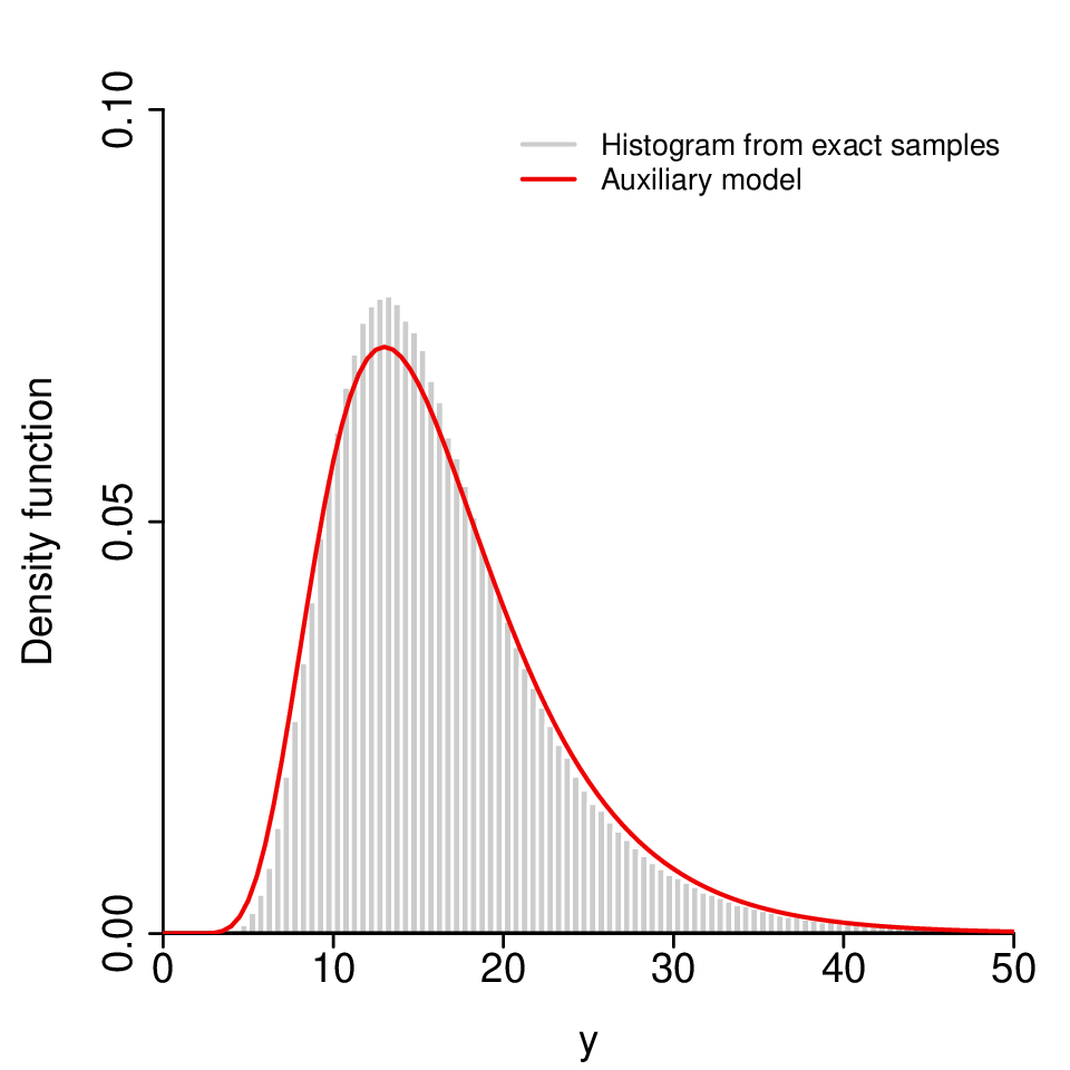
Figure 1a compares the Fenton-Wilkinson lognormal density, $p_{Z}(\bm{y}|\bm{\theta})$, with the true density $p_{Y}(\bm{y}|\bm{\theta})$ at the true parameter values of $\bm{\theta}=(0,1)^{\top}$. The lognormal density is clearly a reasonable match for the true density in this case, although it is slightly more diffuse. However the resulting posterior estimate (shading) is inaccurate, as illustrated in Figure 1b, compared to that obtained under a highly computational ABC rejection sampler (dashed lines) with the vector $\bm{s}=S(\bm{y})={\bm{\theta}}^{*}_{y}$ as summary statistics and with the kernel scale parameter $h$ reduced to a very low level. (The use of the MLE of a tractable approximation as summary statistics is a common approach.) In contrast, the resulting recalibrated posterior approximation (solid lines) appears visually very close to the low-$h$ posterior.

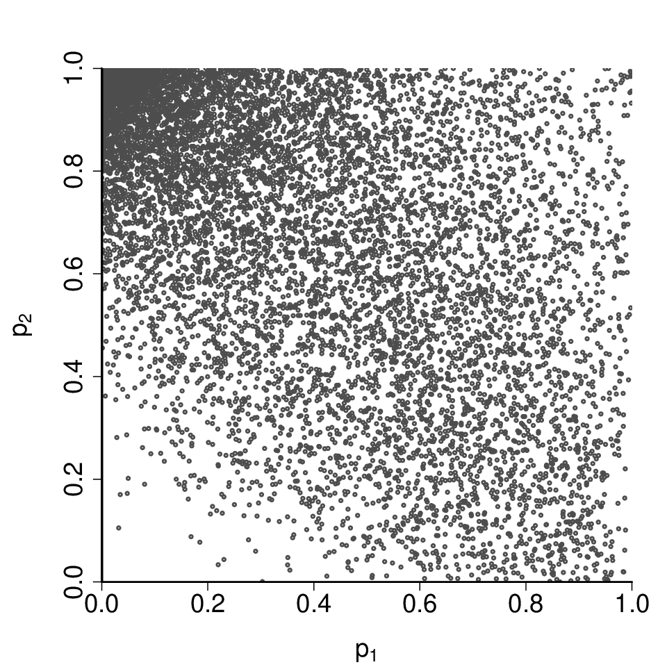
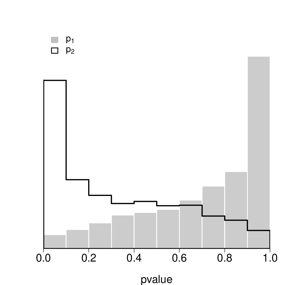
A bivariate scatterplot and univariate marginal histograms of the $\bm{p}=(p_{1},p_{2})^{\top}$ values produced in the recalibration are shown in Figures 1c and 1d. The non-uniformity of the marginal histograms suggests that the Fenton-Wilkinson method overestimates $\mu$ and underestimates $\sigma$ for this analysis, which is supported by the posterior density estimates in 1b. In this case the recalibration procedure corrects these errors successfully. In this analysis, the entire inference process took only a few seconds to complete on a desktop PC, with the computational cost dominated by the optimization process involved in computing ${\bm{\theta}}^{*}_{y}$. In comparison, the cost of recalibration was negligible, as it only involved calculating $\bm{p}$ and quantiles from univariate normal distributions.

In this analysis, we investigate and quantify the effect of recalibration of standard ABC sampler output under various conditions. We consider the simple, deterministic data-generating model $Y=\theta_{1}+\theta_{2}^{2}$, with $\bm{\theta}=(\theta_{1},\theta_{2})^{\top}$, and suppose that $\theta_{1}$ and $\theta_{2}$ have independent $N(0,1)$ priors. For a single observed data point ${\bm{y}_{\mathrm{obs}}}=y$, the resulting posterior mass is then concentrated on the set of points satisfying $\theta_{1}=y-\theta_{2}^{2}$. For the below analysis we adopt ${\bm{y}_{\mathrm{obs}}}=1.$

We follow Algorithm 1, and draw $N=10,000$ samples from the prior distribution, use the full dataset $\bm{y}$ (a single data point) as the summary statistic, and adopt the Epanechnikov kernel $K_{h}$, with $h$ determined by giving the 3,000 samples $\bm{\theta}^{(i)}$ for which $\bm{s}^{(i)}$ is closest to ${\bm{s}_{\mathrm{obs}}}$ non-zero weights $w^{(i)}$ (e.g. [Biau et al. 2015]). The 30% acceptance rate of the algorithm is approximately optimal for regression adjustment ABC in this analysis, in terms of producing the minimum mean square error (MSE) of a particular posterior functional (see below and Figure 3a).

Figure 2a illustrates the regression-adjusted ABC samples in comparison to the support of the true posterior, shown by the solid line. Figure 2b shows the same samples following recalibration, which includes the $\bm{p}$ value regression adjustment of Section 2.4. Standard regression-adjustment ABC is easily able to recover the twisted normal shape of the true posterior distribution, however the ABC approximation error is reflected by the extent of the samples lying far from the true posterior support (the solid line). The recalibrated samples, while still having some deviation away from the true posterior support, visibly produce an improved posterior approximation. This is particularly evident in the lower tail of the $\theta_{2}$ margin.

Figure 2c shows the bivariate distribution of the realised $\bm{p}=(p_{1},p_{2})^{\top}$ values. Here, the univariate marginal distributions are almost uniform, indicating that the marginal posterior distributions of the regression-adjusted ABC posterior approximation are close to the true posterior marginal distributions (c.f. Result 1 and [Prangle et al. 2014]), while the striking dependence structure is a direct result of the form of $\pi(\bm{\theta}|{\bm{s}_{\mathrm{obs}}})$.

More qualitatively, we consider estimation of the posterior expectation $E(\theta_{1}-\theta_{2}|\theta_{1}+\theta_{2}^{2}=1)$ under each of four ABC posterior approximation procedures: standard rejection sampling ABC both with and without regression adjustment, and each of these with a subsequent recalibration adjustment (including a regression adjustment on the $\bm{p}$ values). This computation was repeated 1,000 times and for a range of Epanechnikov kernel scale parameter values $h$, resulting in between 100 and all 10,000 samples with non-zero weight $w^{(i)}>0$ being used for the computation. The log (base 10) mean squared error (MSE) over these 1,000 replicates was recorded. The conclusions of the below analysis were unchanged when other quantities of potential interest such as $P(\theta_{1}>\theta_{2}|\theta_{1}+\theta_{2}^{2}=1)$ were considered.

Figure 3a displays the log of the MSE for each method as a function of the number of posterior samples (out of 10,000). The same quantity based on samples drawn from the exact posterior is illustrated by the dashed line. Each of the ABC based log MSE curves behave in a similar way as the number of posterior samples increases (i.e. as the kernel scale parameter $h$ increases). For small scale parameter values, the log MSE initially decreases as long as the quality of the posterior approximation for each method is high, with the decrease in log MSE achieved through an increase in the number of samples. That is, the high log MSE for low $h$ is primarily driven by Monte Carlo error. At some point, however, with increasing $h$ the quality of the posterior approximation deteriorates too much, and the log MSE increases due to bias in the posterior approximation.

However, the relative performance of each ABC method differs in its performance for low $h$, and the point at which the bias in the posterior approximation begins to dominate the MSE. For low $h$ values standard rejection ABC (light red line) performs as well as the exact posterior distribution until around 1,500 samples. For low $h$, implementing any post-processing method only increases the Monte Carlo error, as these require the estimation of regression parameters and/or marginal distribution functions $\tilde{F}_{j,\bm{s}}(\cdot)$, with more overheads required for recalibration than for regression adjustment. For larger $h$, however, there is a clear benefit to post-processing, with the quality of the regression adjusted posterior approximation (dark red line) meaning that it can reach a lower log MSE for an $h$ equivalent to around 3,000 samples. The recalibrated posterior approximations perform even more efficiently, with the recalibrated regression-adjusted ABC posterior the most efficient of all, achieving their optimum log MSE values at around 5,000 and 8,000 samples. In fact, the minimum MSE obtained by recalibration (recalibrated regression-adjusted ABC) was 0.0002, which is a sizeable reduction from its uncalibrated counterpart of 0.0005 (regression-adjusted ABC) – especially taking into account the theoretical minimum, 0.0001, obtained by exact calculations.

Figure 3b presents the same information as Figure 3a but comparing the recalibration adjusted methods both with and without regression adjusted $\bm{p}$ values (Section 2.4). In this case, adjusting the $\bm{p}$ values clearly improves recalibrated rejection ABC, but recalibrated regression-adjustment ABC is only improved to a small extent. This primarily occurs as the linear regression model assumptions are not reasonable in this region.

In the above analysis, for ease of presentation, the same acceptance rate adopted in steps 1.4 and 2.1 of Algorithm 1 was used when computing the marginal estimates $\tilde{F}_{j,\bm{s}}(\cdot)$ in step 2.2. However, it could be computationally more efficient to use different rates for each step, such as using 30% of the synthetic samples to recalibrate a regression-adjustment ABC based on an acceptance rate of 10%.

References

- Aeschbacher et al. 2012 Aeschbacher, S., M. A. Beaumont, and A. Futschik (2012). A novel approach for choosing summary statistics in approximate Bayesian computation. Genetics 192, 1027–1047.
- Anderson and Coles 2002 Anderson, C. and S. Coles (2002). The largest inclusion in a piece of steel. Extremes 5(3), 237–252.
- Asmussen and Rojas-Nandayapa 2008 Asmussen, S. and L. Rojas-Nandayapa (2008). Asymptotics of sums of lognormal random variabiles with Gaussian copula. Statistics and Probability Letters 78, 2709–2714.
- Barthelmé and Chopin 2014 Barthelmé, S. and N. Chopin (2014). Expectation propagation for likelihood-free inference. Journal of the American Statistical Association 109, 315–333.
- Beaumont et al. 2002 Beaumont, M. A., W. Zhang, and D. J. Balding (2002). Approximate Bayesian computation in population genetics. Genetics 162(4), 2025–2035.
- Biau et al. 2015 Biau, G., F. Céreou, and A. Guyader (2015). New insights into approximate Bayesian computation. Ann. Inst. H. Poincaré Probab. Statist. 51, 376–403.
- Blum and François 2010 Blum, M. G. B. and O. François (2010). Non-linear regression models for Approximate Bayesian Computation. Statistics and Computing 20(1), 63–73.
- Blum et al. 2013 Blum, M. G. B., M. A. Nunes, D. Prangle, and S. A. Sisson (2013). A comparative review of dimension reduction methods in approximate Bayesian computation. Statistical Science 28, 189–208.
- Bortot et al. 2007 Bortot, P., S. G. Coles, and S. a. Sisson (2007). Inference for Stereological Extremes. Journal of the American Statistical Association 102(477), 84–92.
- Cook et al. 2006 Cook, S. R., A. Gelman, and D. B. Rubin (2006). Validation of software for Bayesian models using posterior quantiles. Journal of Computational and Graphical Statistics 15(3), 675–692.
- Drovandi et al. 2017 Drovandi, C. C., K. L. Mengersen, and C. P. Robert (2017). Approximating the likelihood in Approximate Bayesian Computation. In S. A. Sisson, Y. Fan, and M. A. Beaumont (Eds.), Handbook of Approximate Bayesian Computation, pp. in press. Chapman & Hall/CRC Press.
- Drovandi et al. 2015 Drovandi, C. C., A. N. Pettitt, and A. Lee (2015). Bayesian indirect inference using a parametric auxiliary model. Statistical Science 30(1), 72–95.
- Erhardt and Sisson 2016 Erhardt, R. and S. Sisson (2016). Modelling extremes using approximate Bayesian computation. In Extreme Value Modeling and Risk Analysis, pp. 281–306. Chapman and Hall/CRC Press.
- Fan et al. 2013 Fan, Y., D. J. Nott, and S. A. Sisson (2013). Approximate Bayesian computation via regression density estimation. Stat 2, 34–48.
- Fearnhead and Prangle 2012 Fearnhead, P. and D. Prangle (2012). Constructing summary statistics for approximate Bayesian computation: Semi-automatic approximate Bayesian computation. Journal of the Royal Statistical Society. Series B: Statistical Methodology 74(3), 419–474.
- Fenton 1960 Fenton, L. F. (1960). The sum of log-normal probability distributions in scatter transmission systems. IRE Transactions on Communications Systems 8(1), 57–67.
- Frazier et al. 2017 Frazier, D. T., C. P. Robert, and J. Rousseau (2017). Model misspecification in ABC: Consequences and diagnostics. In preparation.
- Gleim and Pigorsch 2013 Gleim, A. and C. Pigorsch (2013). Approximate Bayesian computation with indirect summary statistics. Technical report, http://citeseerx.ist.psu.edu/viewdoc/summary?doi=10.1.1.665.5503.
- Gourieroux et al. 1993 Gourieroux, C., A. Monfort, and E. Renault (1993). Indirect inference. Journal of Applied Econometrics 8(S1), S85–S118.
- Jingxian et al. 2005 Jingxian, W., N. B. Mehta, and Z. Jin (2005). A flexible lognormal sum approximation method. GLOBECOM - IEEE Global Telecommunications Conference 6, 3413–3417.
- Li et al. 2017 Li, J., D. J. Nott, Y. Fan, and S. A. Sisson (2017). Extending approximate Bayesian computation methods to high dimensions via Gaussian copula. Computational Statistics and Data Analysis 106, 77–89.
- Marin et al. 2016 Marin, J.-M., L. Raynal, P. Pudlo, M. Ribatet, and C. P. Robert (2016). ABC random forests for Bayesian parameter inference. https://arxiv.org/abs/1605.05537.
- Martin et al. 2017 Martin, G. M., B. P. McCabe, D. T. Frazier, W. Maneesoonthorn, and C. P. Robert (2017). Auxiliary likelihood-based approximate Bayesian computation in state space models. arXiv preprint arXiv:1604.07949.
- Menéndez et al. 2014 Menéndez, P., Y. Fan, P. H. Garthwaite, and S. A. Sisson (2014). Simultaneous adjustment of bias and coverage probabilities for confidence intervals. Computational Statistics and Data Analysis 70, 35–44.
- Nott et al. 2014 Nott, D. J., Y. Fan, L. Marshall, and S. A. Sisson (2014). Approximate Bayesian computation and Bayes linear analysis: Towards high-dimensional ABC. Journal of Computational and Graphical Statistics 23, 65–86.
- Prangle et al. 2014 Prangle, D., M. G. B. Blum, G. Popovic, and S. A. Sisson (2014). Diagnostic tools for approximate Bayesian computation using the coverage property, Invited Paper. Australia and New Zealand Journal of Statistics 56, 309–329.
- Schwartz and Yeh 1982 Schwartz, S. C. and Y. S. Yeh (1982). On the distribution function and moments of power sums with log-normal components. Bell System Technical Journal 61(7), 1441–1462.
- Sisson et al. 2017 Sisson, S. A., Y. Fan, and M. A. Beaumont (2017). Overview of approximate Bayesian computation. In S. A. Sisson, Y. Fan, and M. A. Beaumont (Eds.), Handbook of Approximate Bayesian Computation, pp. in press. Chapman & Hall/CRC.
- Tran et al. 2017 Tran, M.-N., D. J. Nott, and R. Kohn (2017). Variational Bayes with intractable likelihood. Journal of Computational and Graphical Statistics, in press.
- Wegmann et al. 2009 Wegmann, D., C. Leuenberger, and L. Excoffier (2009). Efficient approximate Bayesian computation coupled with Markov chain Monte Carlo without likelihood. Genetics 182, 1207–1218.
- Wegmann et al. 2010 Wegmann, D., C. Leuenberger, S. Neuenschwander, and L. Excoffier (2010). ABCtoolbox: a versatile toolkit for approximate Bayesian computations. BMC bioinformatics 11(1), 116.