Beam Energy Dependence of Dielectron Production in Au+Au Collisions from STAR at RHIC
Contents
Abstract
At sufficiently high temperatures and baryon densities, nuclear matter is expected to undergo a transition into the Quark-Gluon-Plasma (QGP) consisting of deconfined quarks and gluons and accompanied by chiral symmetry restoration. Signals of these two fundamental characteristics of Quantum-Chromo-Dynamics (QCD) can be studied in ultra-relativistic heavy-ion collisions producing a relatively large volume of high energy and nucleon densities as existent in the early universe. Dileptons are unique bulk-penetrating sources for this purpose since they penetrate through the surrounding medium with negligible interaction and are created throughout the entire evolution of the initially created fireball. A multitude of experiments at SIS18, SPS and RHIC have taken on the challenging task to measure these rare probes in a heavy-ion environment. NA60’s results from high-quality dimuon measurements have identified the broadened spectral function as favorable scenario to explain the low-mass dilepton excess, and partonic sources as dominant at intermediate dilepton masses.
Enabled by the addition of a TOF detector system in 2010, the first phase of the Beam Energy Scan (BES-I) at RHIC allows STAR to conduct an unprecedented energy-dependent study of dielectron production within a homogeneous experimental environment, and hence close the wide gap in the QCD phase diagram between SPS and top RHIC energies. This thesis concentrates on the understanding of the LMR enhancement regarding its M, p and energy dependence. It studies dielectron production in Au+Au collisions at beam energies of 19.6, 27, 39, and 62.4 GeV with sufficient statistics. In conjunction with the published STAR results at top RHIC energy, this thesis presents results on the first comprehensive energy-dependent study of dielectron production.
This includes M- and p-spectra for the four beam energies measured in 0-80% minimum-bias Au+Au collisions with high statistics up to 3.5 GeV/c and 2.2 GeV/c, respectively. Their comparison with cocktail simulations of hadronic sources reveals a sizeable and steadily increasing excess yield in the LMR at all beam energies. The scenario of broadened in-medium spectral functions proves to not only serve well as dominating underlying source but also to be universal in nature since it quantitatively and qualitatively explains the LMR enhancements measured over the wide range from SPS to top RHIC energies. It shows that most of the enhancement is governed by interactions of the meson with thermal resonance excitations in the late(r)-stage hot and dense hadronic phase. This conclusion is supported by the energy-dependent measurement of integrated LMR excess yields and enhancement factors. The former do not exhibit a strong dependence on beam energy as expected from the approximately constant total baryon density above 20 GeV, and the latter show agreement with the CERES measurement at SPS energy. The consistency in excess yields and agreement with model calculations over the wide RHIC energy regime makes a strong case for LMR enhancements on the order of a factor 2 - 3.
The extent of the results presented here enables a more solid discussion of its relation to chiral symmetry restoration from a theoretical point of view. High-statistics measurements at BES-II hold the promise to confirm these conclusions along with the LMR enhancment’s relation to total baryon density with decreasing beam energy.
Zusammenfassung
Die vorliegende Doktorarbeit besteht aus einem Hauptteil (Part I) im Themengebiet der hoch-energetischen Kernphysik und einem Nebenteil (Part II) über Entwicklung und Beitrag von neuen Software Modulen zur Kollaboration und der Öffentlichkeit. Der Hauptteil behandelt das Thema der Energieabhängigkeit von Dielektronen-Produktion in ultra-relativistischen Schwerionen-Kollisionen mithilfe des STAR Detektors (Solenoidal Tracker at RHIC) am Brookhaven National Laboratory in Upton, NY. Im Nebenteil werden zum Einen sieben C++ und Python Bibliotheken für Datenanalyse und Dokumentation vorgestellt. Zum Anderen wird in diesem Teil der Übergang der gesamten 15-jährigen Geschichte des STAR Softwarepakets in ein modernes System der Versionskontrolle beschrieben. Beide Teile sind im Folgenden ausführlich zusammengefasst.
Messung der energieabhängigen Dielektronen-Produktion mit STAR
Der Phasenzustand von Kernmaterie ändert sich mit zunehmender Temperatur
und Baryonendichte (Section 1.1). Die Theorie der
Quanten-Chromo-Dynamik (QCD) hat sich sehr erfolgreich darin erwiesen
[1], die Eigenschaften dieser Phasen vorherzusagen
und zu bestätigen. Im QCD Vakuum sind Quarks und Gluonen darauf
beschränkt als Bestandteile von farb-neutralen Hadronen vorzukommen.
Außerdem ist die globale chirale Symmetrie des QCD Langrangian im Vakuum
spontan gebrochen [2]. Mit diesen beiden Charakteristiken ist die
QCD in der Lage, die grundlegenden Eigenschaften des experimentellen
Hadronenspektrums zu beschreiben [3].
Bei ausreichend hohen Temperaturen und Baryonendichten durchläuft
Kernmaterie den Phasenübergang ins Quark-Gluon-Plasma (QGP), in dem freie
Quarks und Gluonen die Freiheitsgrade bestimmen (Deconfinement) und chirale Symmetrie
wiederhergestellt ist [4]. Diese
fundamentalen Eigenschaften der QCD Materie können in
ultra-relativistischen Schwerionen-Kollisionen untersucht werden
[5, 6]. In den Kernstößen wird ein
verhältnismäßig großes Volumen mit hohen Energie- und
Nukleonendichten produziert, die vergleichbar zu den Bedingungen im frühen
Universum sind (Section 1.2). Während der darauffolgenden
Ausdehnung und Abkühlung durchschreitet die heiße und dichte Materie
mehrere QCD Phasen, bevor sie in die beobachtbaren Teilchen des QCD Vakuums
hadronisiert und ausfriert [7].
Messungen des elliptischen Flusses von Mesonen und Baryonen, zum Beispiel,
geben Aufschlüsse sowohl über die Zeitskala der Thermalisierung des
Mediums als auch über den Grad der kollektiven Expansion
[8, 9]. Es ist allerdings wichtig, (eindeutige)
Signale für die beiden fundamentalen QCD Charakteristiken des
Deconfinements und der Chiralen Symmetrie Restauration zu beobachten und
umfassend zu messen: Wenn Quark-Antiquark () Paare in
einem thermisch ausgeglichenen deconfined QCD Medium annihilieren, sollte man
thermische elektromagnetische Strahlung direkt vom QGP beobachten können;
Änderungen der Spektralfunktion von Vektormesonen im Medium könnten
Vorläufereffekte eines Verschwindens der QCD Vakuumstruktur sein
[10, 11]. Die Diskussion des letzteren Zusammenhangs
(Section 1.3) legt dar, dass eine koordinierte Anstrengung von
theoretischer und experimenteller Seite notwendig ist, um die
Schlussfolgerungen aus den Dielektronenmessungen der -Spektralfunktion
bezüglich (teilweiser) Chiraler Symmetrie Restauration zu stärken.
In diesem Bezug sind Dileptonen ein einzigartiges Werkzeug. Sie durchdringen
das umgebende Medium mit vernachlässigbarer
Wechselwirkung und entstammen
der gesamten Evolution des Systems (Figure 1.6). Die
Verteilungen von invarianter Masse (M) und Transversalimpuls (p)
widerspiegeln ihre zeitlich geordnete Emission und sind daher empfindlich auf
die Evolutionsdynamik des Systems. Insbesondere die Low-Mass- (LMR) und
Intermediate-Mass-Regionen der Dielektronenspektren versprechen jeweils
Zugang zur in-Medium modifizierten -Spektralfunktion und zur effektiven
QGP Temperatur. Für die Extraktion der QGP Temperatur muss allerdings der
Beitrag eines möglicherweise Medium-modifizierten Charm Kontinuums bekannt
sein [12].
Eine Vielzahl von Experimenten an SIS18 (Schwerionen-Synchrotron), SPS (Super
Proton Synchrotron), und RHIC (Relativistic Heavy Ion Collider)
haben die schwere Aufgabe auf sich genommen, diese seltenen Proben in einer
Schwerionen-Umgebung zu messen (Section 1.3.1). CERES
beobachtete als erstes Experiment einen beträchtlichen und
unerklärten LMR Produktionsüberschuss im Vergleich zu einem Cocktail
aus erwarteten hadronischen Quellen [13]. Die NA60 Resultate
von hoch-qualitativen Dimuonen-Messungen haben die verbreiterte
-Spektralfunktion als bevorzugtes Szenario für den LMR
Überschuss und einen partonischen Ursprung für die dominanten Quellen
im IMR identifiziert [14]. PHENIX folgte mit
Dielektronen-Messungen bei höchsten RHIC Energien, die eine bedeutende
Verstärkung des LMR Signals und gute Übereinstimmung der IMR
Produktion mit einem Charm Kontinuum von N-skalierten p+p Kollisionen
aufweisen [15].
Im Gegensatz zu den NA60 Ergebnissen, konnte die Größe der LMR
Signalverstärkung nicht durch existierende Modellrechnungen erklärt
werden - selbst mit Ausnutzung des gesamten verfügbaren Parameterraums.
Messungen der Dielektronen-Produktion bei identischen Energien mit STAR am RHIC
führten zu einer moderateren Verstärkung, die im Einklang ist mit den
NA60 Resultaten und mit Modellrechnungen basierend auf in-Medium
verbreiterten
-Spektralfunktionen [16]. Es sei an dieser Stelle
angemerkt, dass HADES für niedrige Temperaturen und hohe Baryonendichten
das DLS Rätsel mit einem LMR Verstärkungsfaktor von
2-3 bestätigt hat [17, 18].
Diese Vorgeschichte schafft die Voraussetzungen für die umfassende
Untersuchung der Dielektronenproduktion in dieser Doktorarbeit. Ermöglicht
durch die Hinzufügung des Time-Of-Flight (TOF) Detektors im Jahre 2010
liefert STAR ausgezeichnete Teilchenidentifikation, niedriges Materialbudget,
volle azimuthale Akzeptanz bei mittleren Rapiditäten, und breite
p-Abdeckung [19]. Insbesondere mit der ersten Phase des Beam
Energy Scans (BES-I) [20] bietet STAR die noch nie da
gewesene Gelegenheit, eine energie-abhängige Untersuchung der
Dielektronenproduktion innerhalb eines homogenen experimentellen Umfelds
durchzuführen und damit die große Lücke im QCD Phasendiagram
zwischen SPS und höchsten RHIC Energien zu schliessen
(Section 1.4).
Die vorliegende Arbeit konzentriert sich auf die Analyse von
Au+Au Kollisionen bei Strahlenergien von 19.6, 27, 39, und 62.4 GeV, die
während BES-I mit ausreichender Statistik für eine solche
Untersuchung aufgenommen wurden (Section 2.1). In Verbindung mit den
veröffentlichten STAR Ergebnissen bei höchsten RHIC Energien stellt
dies den ersten umfassenden und energie-abhängigen Datensatz bereit.
Angesichts des beträchtlichen Aufwands wird dieser Datensatz der wohl
einzig verfügbare bei diesen Energien in naher Zukunft
bleiben.11
1
STAR wird weiterhin Daten mit hoher Statistik bei
s ¡ 20 GeV während BES-II aufnehmen.
Zu Beginn der Analyse werden geeignete Auswahlkriterien angewandt, um den
Datensatz auf hoch-qualitative Kollisionsereignisse (Events) und
Teilchenspuren zu reduzieren (Section 2.2). Die zusätzliche
Rekonstruktion der Eventebene (Section 2.2.2) ist Voraussetzung
für die statistische Generierung von Untergrund-Paarverteilungen.
Elektronen und Positronen werden durch Kombination von Impuls, Geschwindigkeit,
und Energieverlust gemessen im TOF Detektor und der Time-Projection-Chamber
(TPC) sauber identifiziert (Section 2.3). Dielektronen (e/e Paare)
werden aus der resultierenden Auswahl von Elektronen und Positronen kinetisch
rekonstruiert und Untergrund-Beiträge statistisch abgezogen
(Section 2.4), indem von Same- und Mixed-Event Methoden auf
p-integrierte und -differentierte Weise Gebrauch gemacht wird.
Für den Vergleich zu theoretischen Rechnungen und zwischen Energien
müssen die rohen M- und p-Verteilungen der Dielektronen korrigiert
werden (Chapter 3), um Verluste durch Detektor-Ineffizienzen und Auswahlkriterien zu
beheben. Zu diesem Zweck werden simulierte Teilchenspuren in reale Events
eingebettet (Embedding) und mit denselben Mitteln wie für die
experimentelle Eventrekonstruktion durch den Detektor verfolgt
(Section 3.1). Die Abschätzung von systematischen
Unsicherheiten erfordert den Vergleich von simulierten zu sauberen
experimentellen Verteilungen basierend auf geeigneter Teilchenauswahl. Die
Berechnung von Gesamt-Effizienzen der Spurrekonstruktion und -verfolgung folgt
dem Vorgehen der experimentellen Datenanalyse und benutzt die dedizierte
Teilchenauswahl von Embedding und Experiment (Section 3.2). Die
Spureffizienzen werden schließlich mithilfe einer einfachen
Zwei-Körper Monte-Carlo Simulation in Paareffizienzen übertragen
(Section 3.3).
Die Physik-Interpretation der experimentellen Ergebnisse in dieser Arbeit
(Chapter 5) basiert auf (i) der Simulation hadronischer
Zerfallskanäle, die bekanntermaßen zur Dielektronenproduktion in
elementaren Kollisionen beitragen, und (ii) effektive Modellrechnungen, die
die in-Medium Effekte beschreiben. Ersteres stellt den sogenannten
hadronischen Cocktail dar, dessen Quellen und charakteristischen
Massenregionen in der Einleitung im Zusammenhang mit p+p Kollisionen
vorgestellt und mit früheren Dielektronen-Messungen in
Schwerionen-Kollisionen verglichen werden (Section 1.3). Die
Einzelheiten der Cocktail Simulationen, wie sie für die
energie-abhängige Dielektronen-Produktion in Au+Au Kollisionen bei BES-I
Energien verwendet werden, sind ausführlich beschrieben
(Section 4.1). In der Einleitung (Section 1.3) wird auch der
gemessene LMR Produktionüberschuss über dem Cocktail und dessen
mögliche Verbindung zu Chiraler Symmetrie Restaurierung mittels Hadronic
Many-Body Theory (HMBT) behandelt. Im Simulationskapitel (Section 4.2)
werden einige veranschauliche Einzelheiten und die Ergebnisse dieser
Berechnungen für BES-I Energien diskutiert.
Für die genannten vier Strahlenergien, legt diese Dissertation M- and
p-Spektren vor (Chapter 5), gemessen in 0-80% minimum-bias Au+Au
Kollisionen mit hoher Statistik bis zu jeweils 3.5 GeV/c und 2.2 GeV/c.
Deren Vergleich zu Cocktail Simulationen aus hadronischen Quellen deckt einen
beträchtigen und stetig zunehmenden LMR Überschuss bei allen Energien
auf. Dieser kann weder durch Vakuum /-Spektralfunktionen, die durch
die Feuerball-Expansion propagiert wurden, noch durch die entsprechenden
bloßen Ausfrierungsbeiträge beschrieben werden. Modellrechnungen mit
einer in-Medium verbreiterten -Spektralfunktion auf Grundlage von
HMBT erreichen stattdessen gute
Übereinstimmung sowohl über den gesamten Energiebereich als auch in
der Form der M- und p- Verteilungen. Dieser Beitrag dominiert im LMR
über die Beiträge vom QGP und dient daher im
Allgemeinen gut als zugrunde liegende Ursache des gemessen Überschusses im
gesamten RHIC Energiebereich. Die Beobachtung bedeutet auch, dass der Großteil
der Signalverstärkung durch Wechselwirkungen des -Mesons mit
thermischen Resonanzanregungen in der spät(er)en heißen und dichten
hadronischen Phase geregelt wird.
Die Energie-Abhängigkeit sowohl der M-integrierten und auf invariante
Pionen-Produktion normierten LMR Überschüsse als auch der LMR
Signalverstärkung unterstützen diese Schlussfolgerung. Im Einklang
mit der etwa konstanten totalen Baryonendichte überhalb von 20 GeV weisen
die absoluten Überschüsse keine starke Abhängigkeit von der
Strahlenergie auf. Die Verstärkungsfaktoren des LMR Signals stimmen mit
CERES Messungen bei SPS Energien trotz unterschiedlicher Akzeptanzen
überein - die STAR Daten sind jedoch von höherer Qualität. Die
von STAR gemessene Beständigkeit des LMR Überschusses und dessen
Übereinstimmung mit Modellrechnungen über den breiten RHIC
Energiebereich liefern überzeugende Argumente für
Verstärkungsfaktoren eher im Bereich 2 - 3 als 5 oder mehr.
Die Energie-Abhängigkeit der integrierten LMR Überschüsse
ermöglicht eine interessante Prognose für die zweite Phase des Beam
Energy Scans (BES-II). Im Energiebereich unterhalb von 20 GeV weisen sowohl
Messungen der totalen Baryonendichten als auch -Meson-basierte PHSD
Rechnungen auf eine ungefähre Verdopplung des LMR Überschusses hin
[21, 22]. Messungen während BES-II mit hoher
Statistik sollten ausreichend Genauigkeit bieten, um diese Vorhersagen zu
testen und unser Verständnis der LMR Signalverstärkung sowie dessen
zugrunde liegende Ursache weiter zu kräftigen [23]. Außer
gesteigerter Statistik wird BES-II mit der beabsichtigten iTPC Aufrüstung
feinere Spurverfolgung und verbesserte Fähigkeiten zur Dimuonen-Messung
liefern.
In der gegenwärtigen Untersuchung sind verlässliche
Rückschlüsse auf QGP Strahlung im IMR leider beschränkt durch a)
die vorhandene Statistik, b) die Unsicherheiten in den Wirkungsquerschnitten in Nukleon-Nukleon Kollisionen, und c) die möglichen
Medium-Modifikationen des Charm Kontinuums durch Entkorrelation der
Zerfallsprodukte. Mithilfe der kürzlich
abgeschlossenen Aufrüstungen der HFT (Heavy Flavor Tracker) und MTD (Muon
Telescope Detector) Detektor-Teilsysteme werden
es BES-II Messungen aber ermöglichen, das Charm Kontinuum und damit
indirekt QGP Strahlung zu untersuchen. Dies ist insbesondere wichtig für
den LMR, da der Beitrag zum Gesamt-Cocktail im 0.4 - 0.7
GeV/c Massenbereich von etwa 20% bei 19.6 GeV auf etwa 60% bei 200 GeV
steigt.
Zusammenfassend stellen die STAR Messungen während BES-I hoch-qualitative Datensätze zur Verfügung, die wesentlich für das Verständnis der LMR Signalverstärkung bezüglich ihrer M-, p- und Energie-Abhängigkeit sind. Die Untersuchung der zugehörigen Zentralitätsabhängigkeit in der nahen Zukunft würde die extrahierbaren Ergebnisse vervollständigen und könnte neue Informationen über die Energie-Abhängigkeit der Feuerball-Lebensdauer preisgeben. Das Szenario der in-Medium verbreiterten -Spektralfunktionen erklärt quantitativ und qualitativ die gemessene LMR Signalverstärkung über den breiten Bereich von SPS bis zu höchsten RHIC Energien. Diese Erklärung erweist sich daher nicht nur dazu in der Lage als dominante zugrunde liegende Ursache zu dienen sondern auch als universell in ihrem Wesen.
Der Umfang der dargelegten Ergebnisse erlaubt eine solidere Diskussion im Hinblick auf deren Beziehung zu Chiraler Symmetrie Restauration vom theoretischen Standpunkt aus. Messungen mit hoher Statistik während BES-II verprechen, diese Folgerungen sowie die Relation von LMR Signalverstärkung zu totaler Baryonendichte mit abnehmender Strahlenergie zu bestätigen.
Software Projekte für STAR und Open-Source
Die C++ Softwareklasse StV0TofCorrection (Section 7.1) implementiert
Funktionen, um die Flugzeit von Teilchen aus V (Off-Vertex) Zerfällen
zu korrigieren. Der zugrunde liegende Algorithmus basiert auf der berichtigten
Rekonstruktion der Mutterteilchen. Die Anwendung auf - und
-Zerfälle legt dessen Fähigkeit dar, zusätzlich
Untergrund von anderen Zerfällen zu verwerfen. Außerdem erlaubt die
Klasse dem Benutzer, einen Standardfilter auf die korrigierten Teilchenmassen
anzulegen und damit das Signal-zu-Untergrund Verhätnis zu verbessern. Der
Quellcode dieser Arbeit ist seit Januar 2011 Teil des StBTofUtil [24] Moduls in der offiziellen STAR Code Repositorie. Die neueste
Revision der Implementation ist von Dezember 2013. Ein interner Report wurde
der STAR Kollaboration zugänglich gemacht
[25] 22
2
Dieser Teil der Dissertation wurde
vom DAAD durch ein Auslandsstipendium unterstützt.
.
Die C++ Softwareklasse StBadRdosDb (Section 7.2) wurde im Rahmen dieser
Arbeit entwickelt, um im Laufe einer Analyse bequem Informationen über die
Anzahl der fehlenden Auslese-Boards der TPC zu erfragen. Die Daten der 2010 und
2011 Strahlzeiten werden in zeitliche Perioden (run ranges) mit gleicher
Anzahl fehlender Boards unterteilt und in einem passenden Datenbankformat
gespeichert. StBadRdosDb kann dann benutzt werden, um die zugehörige
Periode für einen spezifischen Run zu erhalten. Dies ist insbesondere
hilfreich für Analysen, die sich auf stabile Detektorbedingungen
während der Strahlzeit verlassen und daher empfindlich auf
run-range-abhängige Effizienzkorrekturen sind. StBadRdosDb wurde der
gesamten STAR Kollaboration bekannt gemacht [26] und
ebenfalls in der STAR CVS Repositorie zur Verfügung gestellt
[27].
Die C++ Softwareklasse StRunIdEventsDb (Section 7.3) wurde
entwickelt, um die Handhabung von Run-abhängigen Untersuchungen
über mehrere Strahlenergien (Part I) zu erleichtern. Für alle
BES-I Energien der Jahre 2010 und 2011 stellt die Implementation eine Abbildung
von einer spezifischen Run Identifikationsnummer zum zugehörigen
Listenindex bereit. Für eine Kombination von Run und Trigger kann
desweiteren die Anzahl an Events für alle Energien abgefragt werden.
Ein weiteres Kapitel im zweiten Teil dieser Dissertation (Chapter 8)
beschäftigt sich mit der Ausführung des Übergangs der zentralen
STAR Code Repositorie von CVS zu git. Es wird vorgeführt, wie die
gesamte Geschichte aller STAR Module mithilfe von cvs2git konvertiert werden
kann. Außerdem wird gerrit als neues Review-System für
zukünftige Code-Änderungen und als Gateway für alle
Interaktionen mit der zentralen Repositorie eingeführt. Dies bezieht die
Bereitstellung der notwendigen Skripten und Anweisungen sowie die
Demonstration
eines Einsatzes des Review-System auf einem entfernten Server mit ein. Als
Ersatz für cvsweb zum Browsen der neuen Repositorien wird cgit vorgeschlagen.
Die Größe und projektinternen Bibliotheksabhängigkeiten machen
die Organisation von Software entwickelt für Physik-Analysen (Part I)
mühsam [28]. Oft werden die ROOT-basierten shared
libraries von länglichen Makros anstatt von kompilierten Programmen aus
aufgerufen, obwohl es die Qualität des Softwareprojekts
erheblich verbessern würde. Das C++ Programm ckon (Section 9.1) wurde daher
entwickelt, um den Arbeitsablauf der Kompilation und Ausführung von ROOT
Analysen zu automatisieren. Mit den Befehlen ckon setup && ckon erlaubt
ckon dem Benutzer, den Erstellungsprozess eines gesamten Softwareprojekts
automatisiert zu durchlaufen, aber gleichzeitig über dessen Ordner-Layout
zu entscheiden. Der Benutzer ist nicht nur vom Makefile-Schreiben befreit
sondern kann auch auf einfache Weise fremden Code oder Dritt-Bibliotheken sowie
eigene Hilfs- und Datenbankklassen mithilfe einer YAML Konfigurationsdatei
einbauen.
Das graphische Darstellungswerkzeug ccsgp (Section 9.2) wurde entwickelt, um Veröffentlichungs-fertige wissenschaftliche Abbildungen mit Gnuplot und Python zu produzieren. Die Repositorie wp-pdf (Section 9.3) umfasst eine Ansammlung an Anweisungen und Software, um — basierend auf denselben AsciiDoc Dateien — simultan eine Website und einen gedruckten Report für den STAR-internen Review-Prozess zu generieren. Das Kommandozeilen-Program rmrg (Section 9.4) erweitert ROOTs hadd Programm [29] mit fehlenden Features und besserer Kontrolle, um ROOT Bäume oder Histogramme zusammenzufügen.
Part I Physics: Energy-Dependence of Dielectron Production in STAR
Chapter 1 Introduction
«We should investigate [novel] phenomena by distributing high energy or high nucleon density over a relatively large volume.»
— T.D. Lee (1974 [5])
1.1 The Phases of QCD
The Standard Model of particle physics [2] comprises a collection of quantum field theories describing the electromagnetic, weak, and strong interactions of subatomic particles with relative strengths at the size of a nucleon according to their coupling constants:
Quantum-Chromo-Dynamics (QCD) [30-34] has emerged [1] as the underlying theory of strong interactions describing the fundamental properties of quarks and their color-exchanging interactions via gluons. Even though QCD has been a very successful theory to predict and guide experimental observations (e.g. [35], jets [36]), some fundamental questions remain unresolved: For instance, the nuclear constituents of ordinary matter are known but it is yet to be understood how they arrange themselves into the composite structures observed in nature. The running coupling constant of QCD separates the low-energy regime (low momentum transfers Q, large distances) from the high-energy regime in which is small enough for QCD to be treated perturbatively, i.e. by Taylor expansion in orders of [37]. This expansion is applicable down to Q 1 GeV/c or above distances of about 0.2 fm which is still about an order of magnitude smaller than the nucleon radius. Hence, the solution of the QCD equations and therefore the behavior of the nuclear force on energy scales relevant for the description of stable atomic nuclei remain unsettled.
Significant progress in this non-perturbative regime has most successfully been made within the computational framework of Lattice QCD as major mathematical constraints 11 1 in form of the numerical sign problem impeding importance sampling. can be avoided at zero net baryon densities and finite temperatures [38, 39]. However, on scales relevant to the internals of the nucleons, i.e. for the study of quark matter phases with quarks and gluons as degrees of freedom, perturbative QCD suggests the existence of asymptotically free (deconfined) quarks and gluons allowing them to escape their confinement into color-neutral hadrons [37]. Hence, under high temperatures and energy densities, the equations of QCD predict that nuclear matter undergoes a phase transition into the so-called Quark-Gluon-Plasma (QGP) [4] — a "soup" in which quarks and gluons constitute the relevant degrees of freedom.
In 2005, theorists and experimentalists [40] claimed the discovery of a strongly coupled QGP (sQGP) sourced in a so-called Color Glass Condensate (CGC) which was critically discussed at the time by the experiments at the Relativistic Heavy-Ion Collider (RHIC, [41]) emphasizing the need for additional measurements of various other variables [42-45]. It turns out that this sQGP behaves much like a perfect fluid with a viscosity near the quantum limit [46] and unlike a weakly interacting plasma as would intuitively be suggested by the small in the perturbative regime of QCD. In recent years, the study of the properties of this dense nuclear matter has been the main focus of the High Energy Nuclear Physics community [47-49].

The QCD phase diagram shown in Figure 1.1a represents
the current conception how strongly interacting nuclear matter evolves into
other phases when varying the thermodynamical environment, namely temperature
T and baryon-chemical potential which is linked to net baryon
density. Reaching a better understanding of the QCD phase diagram has direct
implications on the role of nuclear matter in the cosmos. The part of the phase
diagram at low temperatures and high baryon densities, on the one hand, is
closely related to the dense nuclear matter at the core of neutron stars
[51]. Due to the tiny ratio of baryon to photon number of about
10 (/T) [2], the part at high temperatures and
low densities, on the other hand, corresponds to the thermodynamical path that
the expanding and cooling early universe took microseconds after the big bang.
At moderate temperatures and baryon densities, nuclear matter exists in form of
a Hadron Gas [52] as dictated by the confining long-range nature
of QCD. Around temperatures of about 170 MeV, Lattice QCD predicts the
liberation of the confined quarks to the QGP [53] resulting in a
notable rise in pressure with increasing temperature due to the release of many
additional degrees of freedom (see Figure 1.1c). The
calculation for 2+1 flavors using light up/down quarks and a heavy strange
quark corresponds to the most realistic case for the equation of state
[50]. The calculations in Figure 1.1b at
zero net baryon density [38] also identify the transition to be
of rapid analytical crossover type given the location of the physical quark
masses in the broad range of possible m and m configurations in the
so-called Columbia phase diagram [54].
Even though Taylor expansion in allows Lattice QCD to be extended into the small non-zero regime, effective models like Nambu-Jona-Lasinio [55, 56] need to be employed instead to cover predictions beyond T. However, such models also need to incorporate the second fundamental QGP characteristics after deconfinement, namely chiral symmetry breaking (SB). Chiral symmetry is evident in the zero quark mass limit of the QCD Lagrangian in form of a re-organization of the QCD vacuum in left and right handed contributions with respect to the orientation of spin versus parity. It is spontaneously broken by the QCD vacuum exhibiting a non-zero quark-antiquark condensate () [57], and hence expected to be restored at high temperatures [58]. Spontaneous SB explains the basic features of the experimental hadron spectrum [3], i.e. the manifestation of eight (nearly) massless Goldstone bosons (, K, ) as well as non-degenerated opposite parity isospin multiplets as observed in Figure 1.1d. The effective models used at > T suggest this chiral transition to be of first order for realistic light quark masses [59, 60]. Together with the Lattice QCD predictions at zero , it results in the appearance of a critical point between the crossover and first-order regions. The latter might end in another critical point at low temperatures due to an unclear border between superfluid nuclear matter and superconducting quark matter [61].
The occurrence of the deconfinement and chiral transitions can intuitively be
understood using the MIT bag model [62, 50] which treats
hadrons as objects confining the valence quarks within a finite size of
vanishing : At high temperatures, the
individual bags merge into a single large bag allowing quarks and gluons to
move freely (see percolation models for QCD [63]). Also, the
hadronic bag is larger than the constituent quark bag defined by current quarks
covered in a cloud of virtual quarks and gluons. This has lead to the
speculation of distinct deconfinement and chiral phase transitions with
[64, 65].
The preceding discussion only outlines the most prominent features of the rich QCD phase diagram bearing relevance to the contents and objective of this thesis (Section 1.4). The publications [61] and [66] including the references therein review the phase diagram in dense QCD and at high baryon densities giving rise to additional partially conjectured phase structures like quarkyonic matter, for instance, which shares properties from baryonic and quark matter phases.
1.2 Ultra-relativistic Heavy-Ion Collisions
The quote at the beginning of Chapter 1 [67], recalls T.D. Lee’s suggestion to try restoring the broken symmetries of the physical vacuum temporarily by studying extended environments of high energy or nucleon densities. It was subsequently demonstrated [5, 6] that the latter could be achieved via relativistic heavy-ion collisions which are still to date the only means to recreate nuclear matter in the laboratory as it existed during the early universe. The phase diagram in Figure 1.1a also depicts -T-regions currently reachable by experiments at the Large Hadron Collider (LHC), in RHIC’s top energy and Beam Energy Scan (BES) programs as well as at the future Facility for Antiproton and Ion Research (FAIR) — to name a selected few. The initial phase of the BES program in the years 2010/11 (BES-I) serves the purpose of scanning the phase diagram of QCD, first and foremost, for evidence of the critical point and the first order phase transition. To locate these characteristics of nuclear matter, the considerable capabilities of the Solenoidal Tracker at RHIC (STAR) allow for a multitude of observables like particle production, collective flow, fluctuations, cumulants, jets and others to be measured and studied in BES-I [20]. Consistently combining the resulting various signatures over a wide range of beam energies makes the BES program a powerful tool to explore the s-dependence as well as possible "turn on/off" effects of partonic media.
Figure 1.1a also indicates the according evolution trajectories such a medium takes through the QCD phase diagram while expanding and cooling. To provide the reader with better insights regarding the evolution of a heavy-ion collision, the space-time picture of the subsequential stages are depicted in Figure 1.2 and schematically discussed in the following [68] in terms of the invariant proper time .

Before the collision ( < 0), the incoming nuclei travel at ultra-relativistic speeds and time dilation causes them to appear as pancake-like objects to an observer in the center-of-mass frame. The nuclear constituents within these thin disks are forced by the Lorentz contraction on very small distances at which (color-carrying) gluons have taken over as the dominating content of hadrons [69]. The gluons can then self-generate very high gluon densities via gluon-splitting (condensate) which inversely corresponds to very high transverse momenta making the incoming nuclei effectively behave like gluonic walls. Such a solid-type behavior on short as opposed to liquid-type on long time scales coined the term for this other new form of nuclear matter: color glass condensate (CGC) [70]. The stochastic source of these self-generating high-density gluon fields is hence of basically static nature which allows the parton distributions to be replaced by an ensemble of coherent classical fields for the CGC’s theoretical treatment [71].
The initial scattering at = 0 is followed by so-called hard processes with momentum transfers of typically Q > 10 GeV/c at LHC energies resulting in the characteristic di-jet events [72, 73], for instance. Around 0.2 fm/c, the transverse momentum scale becomes semi-hard with Q 1 GeV/c and the gluons composed in the CGC are liberated generating most of the final-state multiplicity via fragmentation and hadronization of these initial-state gluons. The liberated partons form the non-equilibrium state of partonic matter called Glasma until it thermalizes into the QGP at 1 fm/c [74]. Naively speaking, thermalization occurs when scattering times characterized by small interaction lengths are small compared to expansion times. Such a quick approach to thermalization at about 1 fm/c requires coherent and strong self-interaction of the liberated partons to compete the medium expansion [75]. However, redistribution of energy in spite of being rapidly driven apart only works to a certain degree since the QGP keeps on expanding and cooling. The result is a space-time dependent temperature profile which only allows for local thermal equilibrium to be reached during expansion. The development of thermal equilibrium distinguishes the respective theoretical treatment of Glasma and QGP via viscous and ideal hydrodynamics [76] which describe the medium’s expansion and flow, thus referring to the fluid’s long-range behavior.
At 10 fm/c, hadronization traps quarks and gluons inside color-less
hadrons corresponding to the previously discussed phase transition into a
Hadron Resonance Gas (HRG). The continuously expanding and cooling
HRG subsequently undergoes two conceptually different so-called freeze-out transitions [7]: (i) a chemical freeze-out stopping inelastic
processes that change hadronic species into each other and hence freezing
hadronic abundances, and (ii) a thermal freeze-out at which all
momentum-changing interactions, i.e. also all elastic collisions, cease. The
cross section of the abundance-changing inelastic hadron-hadron reactions is
(usually much) smaller than the total cross-section which drives all
momentum-changing and hence thermally equilibrating reactions. This makes it
increasingly harder for inelastic reactions to keep up with the continuously
decreasing density. They hence become unlikely earlier during the medium
expansion than elastic reactions, and thus
cause the chemical freeze-out to occur at higher temperatures than the thermal
freeze-out [77]. The latter happens at 20 fm/c when the
HRG cannot keep the local thermal equilibrium intact anymore. Freely streaming
particles are then allowed to escape to the detector measuring momentum
distributions that are expected to be the same as the thermal distribution in
the very late-stage expansion [78]. Note that, for RHIC (7.7 -
200 GeV) and SPS (160 - 200 AGeV) energy regimes, the chemical freeze-out
temperature is close to the critical temperature of the deconfinement
transition. At energies covered at the Alternating Gradient Synchrotron (AGS, <
11 AGeV), however, the chemical and thermal freeze-out temperatures approach
each other and finally coincide at energies measured at the Heavy-Ion
Synchrotron (SIS18, < 2 AGeV) [79].
An important concept in the evolution of heavy-ion collisions is the aforementioned development of a collective motion called flow [80]. In the simplified case of a (strictly) central collision, the interaction zone is circular when viewed along the incident beam directions. The constituents rescattering in the expanding nuclear liquid move outward collectively in a radially isotropic manner typically referred to as radial flow [81]. The according radial expansion velocity can be extracted from the paramaterization of the Blast-Wave model to final-state hadron p spectra [82] which are a result of inherently isotropic thermal emission at temperature T and radial flow. The latter is reflected in the definition of the initial effective temperature of the medium [83, 84]:
The initial overlap zone of two non-centrally colliding nuclei, illustrated in Figure 1.3 (left) [85], is usually of elliptic shape which results in a higher pressure gradient along the shorter direction than along the longer direction. Rescattering thus causes the constituents of the liquid to collectively flow faster in the shorter direction effectively converting the initial spatial into a momentum anisotropy. The azimuthal anisotropy in flow velocity also reveals the self-quenching nature of this so-called elliptic flow as it drives the matter toward a spherical shape. Elliptic flow is characterized by the second Fourier coefficient v in azimuthal multiplicity distributions of final state hadrons [8, 9]:
The chronological build-up of elliptic flow during the expansion is shown in Figure 1.3 (right) using the v measure. The full magnitude of the elliptic flow only develops late(r) in the evolution with the specific timing depending on the effective parton scattering cross sections. Hence, particles created early in the evolution and embedded in this anisotropically expanding medium experience no significant flow, yet. The early saturation of elliptic flow well before the hadronization transition is also indicative of the thermalization to happen on the quark rather than the hadronic level [86].

In summary, Figure 1.2 reiterates the similarity of the space-time picture of a heavy-ion collision to Big Bang cosmology and the related discussion identifies a few fundamental questions that need particular attention in the context of heavy-ion collisions — especially if one wants to prove the creation of a QGP [87, 44]. First, whether thermal equilibrium is reached through sufficient rescattering during the initial stage of the collision. Measurements of elliptic flow at RHIC reveal a magnitude of collective expansion that indicates thermalization time scales of less than 1-2 fm/c and hence, justify the characterization of the medium using bulk thermodynamic variables [88]. Second, whether a distinctive footprint for individual partons can be identified. Number-of-constituent (NCQ) scaling holding up for mesons and baryons suggests a collectively expanding partonic source [89, 90]. Third, signals of the two fundamental QCD characteristics, chiral symmetry restoration and deconfinement, need to be comprehensively studied. For the latter characteristic, detection of direct thermal electromagnetic radiation as expected from annihilation in a thermally equilibrated deconfined QCD medium, would provide one of the desired smoking guns. Another would be to unequivocally measure the disappearance of the vacuum consequences of spontaneous SB in the QCD medium (see Figure 1.1d and Section 1.1).
As will be discussed in the remainder of this introductory chapter, both signatures might be accessible via dileptons which are regarded as golden probes of the early stages due to their bulk-penetrating electromagnetic nature. To cover the various aspects of these striking final-state ingredients of a heavy-ion collision, Section 1.3 further motivates the study of dilepton production including a recapitulation of its experimental and theoretical status. Section 1.4 concludes the introduction with a brief overview of the thesis and its objective.
1.3 Dileptons as Bulk-Penetrating Electromagnetic Probes
The precise measurement of the - and a-mesons’ spectral functions in hadronic decays at the Large Electron-Positron collider (LEP) [91] is shown in Figure 1.4 (left), underlying the vector-axialvector (V-A) splitting of about 500 MeV in Figure 1.1d. It exhibits a clear separation of the respective pole masses as expected from spontaneous SB in the QCD vacuum. In a simplified picture, two scenarios can be distinguished for the degeneration of the chiral partners in a quark matter environment (Figure 1.4 right, [87]): (i) the a pole mass drops to the mass and/or they approach each other, hence keeping the resonant strucure intact, or (ii) the resonances "melt" down to approach the according production rates from perturbative QCD. The clarifying study of the fate of chiral symmetry and its manner of possible restoration in dense states of nuclear matter, thus requires experimental access to the so-called in-medium spectral functions of the chiral partners.

However, the relation of medium-modifications of vector meson spectral functions to chiral symmetry restoration (SR) is not straight-forward. Spectral functions need to be connected, on the one hand, to the order parameter of the chiral transition, namely (a reduction in) the condensate, and, on the other hand, to the measured dilepton yields emanating from the entire fireball evolution. This paragraph follows the arguments in [10] (Section 2.7.1) and [11] in an effort to make the connection that allows dilepton production measured in heavy-ion collisions to be interpreted with respect to SR.

Qualitatively, the relation can be retraced through the discussion of the model-independent (T,)-dependence of the chiral condensate in a pion or nucleon gas at low and T [92-94]:
with the pion decay constant, the (scalar) density and the sigma commutator of hadron h. In the non-relativistic limit, denotes the scalar quark density in the hadron. The expression illustrates that SR is an additive effect since every hadron contributes a certain decrease to the quark condensate according to its , with being produced through thermally excited hadrons [94]. The expression has been generalized for a hadron resonance gas in leading order of density, also taking care of hadronic interactions in a manner consistent with chiral symmetry. In other words, thermal resonance excitations in the hadron gas give rise to the so-called "vacuum cleaner" effect since the resonances’ quark content "sweeps up" the chiral condensate of the vacuum [11]. Together with Figure 1.5, this shows that presence of hadrons alone already results in the reduction of the chiral quark condensate consistent with ab-initio Lattice QCD calculations. The connection to spectral functions becomes clear when studying the mechanisms of the effective hadronic model in Section 4.2 and [95] that are required to comply with the results of the dilepton measurements introduced in Section 1.3.1 and especially with the results of this thesis (Chapter 5). In short, the components that underlie the preferred scenario of a broadening of the -meson’s spectral function, are (i) the modified coupling of its pion cloud to the medium (), and (ii) its direct interactions with the mesons and baryons in the heat bath exciting further resonances (MB). Hence, thermal resonance excitations driving the reduction of the chiral condensate are actually one of the processes causing the -broadening (in addition to chiral mixing through the pion cloud). This close relation of (partial) SR and spectral function is further strengthened by the fact that the and MB medium effects find their counterparts in the term since it decomposes into short- and long-distance contributions from the hadron’s quark core and pion cloud, respectively [96].
Taking the direct approach and measuring the a meson in the medium is experimentally difficult due to its low production rates and broad width. Instead, a coordinated procedure has to be followed to quantitatively connect the chiral quark condensate to measured dilepton yields through the meson’s spectral function [10]: On the theoretical side, the vector and axial-vector spectral functions are calculated within a chirally invariant model carefully constrained by basic symmetry principles using effective vertices in agreement with available data. Using Weinberg sum rules, temperature-dependent pion decay constants and quark condensates can be deduced and compared for consistency with Lattice QCD results. The spectral functions are propagated through a realistic model for the fireball expansion taking into account measured hadronic observables (e.g. v). On the experimental side, this enables the detailed comparison to data with respect to centrality-, -, mass- and p-dependence. Besides centrality, this thesis covers these pivotal ingredients and hence tightens the connection for dilepton data to be interpreted in terms of SR. Since spectral functions are difficult to obtain in Lattice QCD in the near future, this approach is the only way to enable another leap forward in dilepton physics.
Vector mesons are generally a good choice for the in-medium spectroscopy of a quickly expanding and cooling fireball. As indicated by the life times listed below, short-lived resonances such as the -, - and -mesons decay on time scales very similar to the evolution of a heavy-ion collision (cf. Figure 1.2). The long-lived pseudo-scalar - and -mesons, on the other hand, decay long after freeze-out and hence, are not suitable for the study of the early-stage QCD medium.
| 1.3 fm/c | 1.7 fm/c | 23 fm/c | 46 fm/c | 151 pm/c | 26 nm/c |
Due to the matching quantum numbers , Vector Meson Dominance [97] also allows vector mesons to couple to virtual photons which in turn directly decay into dielectrons ( pairs) and dimuons ( pairs) collectively called dileptons. The electromagnetic nature of their interactions causes interaction lengths much larger than the fireball life time rendering final-state interactions negligible. Hence, dileptons can serve as pristine probes allowing for direct and undistorted access to the properties of in-medium spectral functions which makes them the most promising candidates to conduct these studies. Note that, even though -baryons exhibit life times comparable to the -meson, such in-medium information would be lost in the respective hadronic decay channels and . The decay products suffer rescattering in the fireball which basically restricts their sensitivity to the break-up stages of the collision.

As visually depicted in Figure 1.6, dielectrons also emanate from the initial hard scattering via Bremsstrahlung and from the QGP phase via electromagnetic (thermal) radiation in addition to the decays during hadron gas and freeze-out phases. Being thus created throughout the entire evolution of the hot dense medium, dielectrons can be considered bulk-penetrating probes and provide dynamic as well as direct information about their original heavy-ion collision stage encoded in their invariant mass (M) and transverse momentum (p). At this point, it is illustrative to discuss the prevalent features of a simulated dielectron invariant mass spectrum in p+p collisions as shown in Figure 1.7 and compare to the expected sources of dielectron production in heavy-ion collisions. There are multiple categories of electromagnetic radiation and background sources at play contributing to different invariant mass regions of the "physical" spectrum. It can generally be concluded that in heavy-ion collisions, earlier creation times correspond to higher temperatures and thus to higher dielectron invariant masses and vice versa.

The High-Mass Region (HMR, M > 3 GeV/c) is primarily occupied by yields from the prompt production during the primordial nucleon-nucleon collision. Drell-Yan annihilation of quark and antiquark of two passing hadrons dominates over thermal emission in this region. Hidden heavy flavor vector mesons (J/, ’) appear on top of this continuum that also has contributions from semi-leptonic weak decays of B-mesons and -baryons originating from back-to-back pairs and hence, resulting in correlated dileptons.
The Intermediate-Mass Region (IMR, 1.1 < M < 3 GeV/c) also exhibits a continuous yield of correlated pairs from semi-leptonic decays of charmed mesons competing in a heavy-ion environment with thermal radiation via annihilation from the QGP. With contributions from possibly medium-modified correlated charmed decays known, an initial effective temperature of the fireball can be deduced in this region from the slope of dielectron m spectra given sufficient statistics. Due to the scarcity of electromagnetic probes, the latter impedes such a measurement even at SPS or lowest RHIC energies where the cross sections fall off steeply.
In the Low-Mass Region (LMR, M < 1.1 GeV/c), dielectron production is dominated by the decay products from final-state hadronic sources culminating in a cocktail of light pseudo-scalar and vector mesons (,,’,,,). Electromagnetic radiation due to (multiple) reinteractions in the hot and dense HRG populates this region and could provide information about in-medium modifications of the vector mesons’ spectral function properties. Modifications of the dielectron rates and their integration over the fireball evolution as well as consequences on the invariant mass spectrum are addressed in the context of this thesis within an effective multi-body hadronic theory in Section 4.2.
1.3.1 Measurements of Dilepton Production
The challenging measurement of dilepton production has been an active field of
research in experimental high energy nuclear physics through multiple
generations of detectors at colliders and fixed-target machines since the
1990’s. The reader is referred to the main part of the thesis for details on
the general analysis and simulation techniques employed to arrive at the
spectra presented in the following. Here, we concentrate on the results of
selected influential measurements and their current interpretations and
conclusions leading up to the important contributions of this thesis to the
progress of dielectron physics.
The CERES and NA45 collaborations [13, 98-100] first reported an unexplained LMR excess yield in S+Au collisions while achieving excellent agreement of cocktail simulations and data in p+N collisions (Figure 1.8a). However, follow-up comparisons of measured LMR invariant mass spectra with calculated dropping-mass and broadening spectral functions of the -meson in Pb+Au collisions, did not allow for the distinction of the two scenarios. The emergence of high-quality dimuon measurements in In+In collisions by the NA60 collaboration [14] significantly accelerated the progress by clearly favoring the broadened spectral function scenario for the modifications of the -meson driven by (multiple) baryonic interactions in the hot hadronic phase (Figure 1.8b). The tail above the -mass can be described by 4-mixing, correlated charm and QGP contributions [101]. Also particularly interesting are the conclusions that can be drawn from NA60’s measurement of the effective temperature T and its mass dependence in Figure 1.8c. The steady rise up to M of about 1 GeV/c is consistent with the radial flow expected from the hadronic emission source . The sudden drop and hence absence of significant flow above 1 GeV/c, however, suggests the partonic emmission via as dominant source. Accumulation of further evidence as discussed in [14], is even consistent with the interpretation of the excess dimuons as thermal radiation. This not only triggered renewed attention to dilepton physics by the theory community, but also independent and dedicated high-accuracy measurements of the dielectron decay channels at top RHIC energy — first by PHENIX and recently complemented by STAR.


The PHENIX detector system has measured invariant mass and
transverse momentum spectra in d+Au collisions and seen very good agreement of
the data with next-to-leading order perturbative QCD calculations over the
entire accessible phase space [104]. Hence, any enhancement seen in the heavy-ion
collisions is not due to cold nuclear matter effects. More importantly, PHENIX
has also published dielectron invariant mass spectra in Au+Au collisions
[15] exhibiting a significant LMR enhancement of more than a factor
of 5 over an expected cocktail of hadronic sources
(Figure 1.9a). None of the scenarios for in-medium
spectral functions of the vector mesons could satisfactorily explain the
magnitude of the enhancement, even by exhausting the full parameter space
allowed. Same is true for PHSD calculations in which neither the incorporated
hadronic nor partonic sources were able to account for the enhancement observed
by PHENIX. It is interesting to note, that the latest dielectron measurements
by PHENIX using the novel Hadron-Blind Detector (HBD) show a more moderate
enhancement factor of 2-3 for the 20-40% centrality bin [105]. It
remains to be seen whether the large enhancement of the original measurement
bears up in the future since the most central bin of the HBD measurement, to
which most of the enhancement has been attributed, has not been shown to date.
As detailed in Section 1.4, STAR has in recent years entered the
landscape of dielectron measurements enabled by major upgrades to this large
acceptance mid-rapidity (multi-purpose) detector.
Figure 1.9b shows STAR’s main results of the very recently
completed analysis of dielectron production in Au+Au collisions at top RHIC
energy [16]. The statistical quality of the measurement allowed
STAR to observe an enhancement factor of about 1.8 in the mass region 0.30-0.76
GeV/c which is significantly lower than reported by PHENIX. Neither
comparisons of cocktail simulations nor of production yields within PHENIX
acceptance revealed any explanation for the discrepancy in the magnitude of the
LMR excess. A detailed comparison of the LMR invariant mass shapes shows that
the data disfavors a pure vacuum- spectral function for the excess but is
in reasonable agreement with broadened and QGP contributions calculated
within hadronic multi-body as well as PHSD models. This conclusion further
supports the NA60 findings in size and shape. When split in -, -
and -like mass regions, the data over cocktail ratios in the latter two
can be reproduced by the cocktail calculations as opposed to the ratio in the
-like region which is reasonably well described by the aforementioned
models and weakly dependent on the number of participants (N, centrality)
and transverse momentum. A power-law fit to the N-scaled -like
dielectron excess results in an exponent of 0.54 0.18 possibly indicating
sensitivity to QCD medium dynamics like the lifetime of the HRG phase (see
[106]).
For completeness, we also need to discuss measurements of dielectron production in the energy range of normal to moderate temperatures and baryon densities. One of the early measurements in 1.04 AGeV Ca+Ca collisions by the DiLepton Spectrometer (DLS) at the BEVALAC [107] compares dielectron invariant mass distributions to freeze-out decays as well as in-medium modified - and -mesons. While reasonably described by at SPS energies [101], neither the dropping mass nor the broadened in-medium spectral function scenario can account for the considerable excess yield in the low mass region [108, 109] which led to the so-called "DLS-puzzle". The second-generation High Acceptance Di-Electron Spectrometer (HADES) was subsequently built in an effort to systematically study this excess with high precision in the SIS18 energy regime. Taking into account the different acceptances, HADES was able to confirm the DLS measurements in its invariant mass and transverse momentum dependence for 1 and 2 AGeV C+C collisions [17, 18]. The HADES findings further show that such light collision systems can in first order be described as an isospin-averaged (incoherent) superposition of elementary N+N processes (Figure 1.9c). However, in the heavier collision system of Ar+KCl at 1.76 AGeV the -subtracted invariant mass spectrum exceeds this N+N reference by a factor of about 2.5 to 3 between 0.15 and 0.5 GeV/c (Figure 1.9d). The excitation function covered by the DLS and HADES experiments indicates that the excess closer resembles the scaling of pion rather than production. Hence, the interpretation of dielectron production in the regime of 1-2 AGeV bombarding energies requires a better theoretical understanding of the relevant N resonances and their -meson coupling.
1.3.2 Underlying source of Dilepton Enhancement
The final part of this section is dedicated to the empirical discussion of a few theoretical, partly data-driven observations that collectively support the interpretation of the experimental results as thermally emitted dileptons [110]. The purpose is not to provide a complete and resilient overview but rather briefly describe the interplay of a few theoretical points which pinpoint the observed dilepton emission to temperatures around the chiral transition. It provides an instructive exercise since the main conclusion of this thesis plays an integral part in the argumentation.

Due to its unique connection to theory, dilepton invariant mass spectra
directly reflect the thermal emission rate (see Section 4.2.1). The slopes of the dashed lines in
the continuum region of the NA60 dimuon measurements in
Figure 1.10a reveal an emission temperature of about 150 MeV or
at least between 130 and 170 MeV. This temperature range happens to correspond
to the temperature of the chiral transition T.
Figure 1.10b studies in-medium hadronic and QGP contributions
for an equation of state (EoS) with a first-order phase transition at T 180 MeV with respect to a Lattice EoS with T at 170 MeV. The lower
T is balanced by enhanced QGP and depleted hadronic contributions resulting
in almost identical low-mass yields and corroborating a predominant emission
source around T. Also, an effective excess temperature of 220 MeV as well
as rather large flow expansion velocities (0.3) both extracted from
direct photon spectra measured by PHENIX, suggest a "later" emission at T
220 MeV / 1.35 160 MeV T. Theoretically, one observes that the
in-medium -meson rates smoothly "melt" into the according rates from QGP
continuum radiation. Experimentally, the NA60 data has quantitatively confirmed
the broadened spectral function scenario as explanation for the low-mass
excess yields.
Since, as previously discussed, the hadronic in-medium spectral functions
are related to the condensate, the development of a pion
cloud and excitation of baryonic as well as mesonic resonances as mechanisms
underlying this "-melting", are possibly precursor to the dynamic
restoration of chiral symmetry. The preceding theoretical and experimental
observations, as a whole, allow the authors of [110] to speculate
about a three-fold degeneracy of contributions from in-medium HRG,
perturbative QCD and Lattice QCD convening at the chiral phase
transition temperature.
It is crucial, however, to study the dilepton LMR enhancements for various regions of the QCD phase diagram and establish the degree of universality of in-medium vector meson modifications as underlying source. In anticipation of the results, this thesis reports on the extensive energy-dependent measurements during STAR’s BES-I which indeed indicate the universal character of this scenario (see Chapter 5). Hence, the study of emission temperature and in-medium scenarios results in the important observation that spectral slopes, yields and flow of low-mass dileptons at SPS and RHIC point toward a universal underlying source with average emission temperatures of about 150 MeV coinciding with T.
However, there are caveats that need to be kept in mind. It is important to also identify conditions in a heavy-ion environment under which these medium effects turn off. While peripheral collisions are challenging in this regard since the dense hadronic phase still persists, high(er) p data like the NA60 dimuon measurements or elementary projectiles on cold nuclei like +AeeX by CLAS are promising candidates [111]. Last but not least, a thorough theoretical framework needs to relate the measured spectral functions to its chiral partner a to convincingly address the long-standing question of chiral symmetry restoration. Progress in this direction has recently been made in [112].
1.4 Thesis Objective and Overview
As later outlined in Section 4.2, the most distinct features of
electromagnetic radiation from the hot hadronic phase are unfortunately hidden
by the according hadronic freeze-out decays. However, model calculations still
predict about 50% reduction in the / region and more importantly,
about a factor of two enhancement at 0.5 GeV/c when comparing a broadened to
a vacuum-like spectral function for the dielectron spectrum from direct decays
of , and over the fireball evolution
[113, 87]. The / resonances appear to be less
susceptible to the different scenarios. The preceding introduction has argued
that theory can connect these modifications to chiral symmetry restoration with
sufficient experimental data at its disposal. However, the accuracy required to
test the respective differences from various scenarios in the () spectral
function, is experimentally very challenging.
The completion of the Barrel Time-of-Flight detector (TOF) in 2010 has allowed
STAR to play an important role in the study of dielectron production
[16, 114, 115] with excellent particle
identification, low material budget, full azimuthal acceptance at mid-rapidity,
and a wide momentum coverage [19, 116, 117]. STAR
is thus one of the most versatile mid-rapidity detectors currently available to
the High Energy Nuclear Physics community. For instance, TOF efficiently
rejects slow hadrons and provides pure electron identification together with
the energy loss measured in STAR’s Time-Projection-Chamber (TPC), which makes
the two detectors the primary subsystems employed in dielectron analyses at
STAR. In particular, combined with the first phase of the Beam Energy Scan
Program (BES-I, [20]), STAR presents the unprecedented
opportunity to map out a significant portion of the QCD phase diagram within a
homogeneous experimental environment.
The objective of this thesis in the main Part I is to present STAR’s novel
and successful endeavor extending the dielectron measurements from top RHIC
energies down to the SPS energy regime. The results of this thesis therefore
not only close a wide gap in the QCD phase diagram, but also provide the first
comprehensive dataset of dielectron measurements with respect to energy
dependence and experimental environment. In the particular context of the
dielectron analyses presented in this thesis, STAR aims to look for
energy-dependent changes in the in-medium spectral function modifications and
QGP radiation, possibly identifying the underlying universal nature of the
respective dielectron emission source(s). Only by varying beam energy and
accessing different regions of the phase diagram, we can objectively verify
conclusions reached for energies at which a QGP is or is not expected to form.
This fundamentally distinguishes the efforts in this thesis from dielectron
measurements previously undertaken. The discussion in Section 1.3 in
particular, has identified such measurements as crucial experimental input to
explore the connection between measured dilepton yields and chiral symmetry
restoration.
The thesis is outlined as follows. Chapter 2 starts out by briefly introducing the concepts of RHIC as well as important aspects of the STAR detector setup relevant to dielectron analyses. It continues with the key elements of the experimental raw data analyses ranging from event and track selection including particle identification to pair reconstruction and background subtraction. Chapter 3 presents the procedure employed to derive and apply corrections due to detector inefficiencies. Chapter 5 discusses the obtained results including new and energy-dependent invariant mass spectra as well as p spectra in comparison to the simulations and model calculations of Chapter 4. In the end, Chapter 6 summarizes the main results of the thesis and gives an outlook on the role of dielectron measurements in the current STAR upgrades, the future second phase of the Beam Energy Scan program (BES-II), and CERN’s LHC. Preliminary versions of the results in Chapter 5 have been presented at various major conferences in recent years, and published in the respective proceedings [118]. Papers based on the results of this thesis are in preparation to be published in the journals Physical Review Letters and Physical Review C.
Additional parts on software (Part II) and hardware (Chapter 11) projects developed within the framework of this thesis contain a multitude of contributions to the STAR 22 2 a selection will possibly be published as STAR notes in the future and Open-Source community as well as the inital development of a Xe-Excimer Lamp designed to enable pad-by-pad efficiency corrections for the RICH detector of the HADES experiment.
Chapter 2 Data Acquisition and Analysis
This chapter discusses the complex but integral part of gathering and analyzing the (raw) data required to perform an energy-dependent measurement of dielectron production at the Relativistic Heavy Ion Collider (RHIC). Section 2.1 briefly presents relevant aspects of experimental setup and data acquisition by means of the Solenoidal Tracker at RHIC (STAR). In Section 2.2, the datasets used in this thesis are introduced and suitable selection criteria are discussed to reduce the data to high-quality collision events and particle tracks. The separate reconstruction and analysis of the event plane described in Section 2.2.2 is a prerequisite for the statistical generation of background pair distributions. The procedure to cleanly identify electrons and positrons using STAR’s detector subsystems Time-Of-Flight (TOF) and Time Projection Chamber (TPC) is discussed in Section 2.3 along with the resulting sample purities. Dielectrons (e/e pairs) are reconstructed and background contributions substracted statistically in Section 2.4 by employing same and mixed event techniques in p-integrated and -differential manner. Note that corrections to account for efficiency losses in the detector and to be applied on the raw spectra are derived in Chapter 3.
2.1 Experiment: RHIC and STAR

It is beyond the scope of this thesis to give a complete introduction to neither the functionality of heavy-ion accelerators nor the technology used to build the detectors around the collision zone. Since excellent reviews about RHIC and STAR already exist [120], this section gives overviews merely outlining the general concepts of the two and concentrates on some additional details relevant to dielectron analyses. Where appropriate the reader is referred to references containing in-depth information.
The scenario to feed Au ions into RHIC using an injector chain of accelerator rings is sketched out in Figure 2.1 [119]. The Tandem Van de Graaff as well as the Booster and the Alternating Gradient (AGS) synchrotrons are pre-existing hadron accelerators at the Brookhaven National Laboratory (BNL) [121] that provide three different stages of increasing beam energy after each of which the Au ions are partially stripped of their electrons to adjust their charge to the according next-stage ring diameters and intended energies. The Tandem [122] uses its characteristic two-stage acceleration mode including mid-way electron stripping to boost Au ions from the sputter ion source [123] to an energy of 1 MeV/u. A charge state of +32 is subsequently selected by bending magnets for the delivery via the Heavy Ion Transfer Line [124] to the Booster Synchrotron [125, 126] in which the Au ions are accelerated to 95 MeV/u. Au ions exit the Booster for the final step of acceleration in the AGS [127] to an energy of 10.8 GeV/u before bunch-wise injection into RHIC as Au via the AGS-to-RHIC transfer line [128]. RHIC consists of a pair of superconducting rings with 3.8 km circumference capable of accelerating and storing two counter-circulating gold beams with energies up to 100 GeV/u each [129]. The rings intersect at four points along the circumference allowing for a complementary set of detectors [130] to conduct experiments using relativistic heavy ion collisions. Each experiment operates a pair of Zero-Degree Calorimeters (ZDCs) [131, 132] as a common detector subsystem on either side of and close to the respective interaction zones. The ZDCs detect neutron multiplicities from the collisions and enable the accelerator staff to monitor luminosity and locate collision vertices ("steering"). For more details on RHIC, the reader may want to use [133] as an entry point.
The data for the energy-dependent analysis of dielectron production presented here has been obtained by means of the STAR detector [134, 135]. The STAR detector serves the study of a very broad physics program ranging from high-density QCD, over the proton’s spin structure to ultra-peripheral collisions via electromagnetic interactions of passing ions. Such a program requires a suite of multi-purpose and complementary detector subsystems. Figure 2.2 shows a graphical rendering of the STAR detector with its subsystems Endcap [136] & Barrel [137] Electromagnetic Calorimeters (EEMC & BEMC), Beam-Beam Counter [138] (BBC), upgraded pseudo Vertex Position Detector [139, 140] (upVPD), and Magnet [141]. Also depicted are TPC and TOF, the combination of which is particularly important for the study of dielectrons and discussed to some detail in Section 2.1.1 followed by STAR’s Data Acquisition (DAQ) and Trigger systems in Section 2.1.2.

2.1.1 TPC and TOF
The cylindrical Time Projection Chamber (TPC) [143] constitutes the very heart of the STAR detector system measuring 4 m in diameter as well as length, and stretching from 50 to 200 cm in radial distance from the beam axis. Stable and unstable particles emanate from the collision zone located approximately in the center of the TPC and traverse through the covered volume filled with P10 gas (10% methane, 90% argon). Along their path, the particles ionize the P10 gas leaving behind a track of released secondary electrons. A thin conductive membrane at the center of the TPC, the concentric field-cage cylinders, and the end caps define a uniform electric field of 135 V/cm which induces a drift of the electrons along its field lines toward the readout caps at both ends of the chamber. P10 gas is a well-established choice for this purpose since it exhibits fast drift velocities at comparably low electric fields. The charge of the drifting electrons, registered when they reach the TPC’s readout plane, allows for the measurement of a track segment’s x/y and z coordinates through its projection into two dimensions and the elapsed drift time, respectively.
The TPC is furthermore installed inside a large solenoidal, room-temperature magnet providing a uniform field of up to 0.5 T along the z-direction (beam axis). In addition to the spatial reconstruction, the charged particle’s momentum can hence be derived from the track’s curvature in the magnetic field enabling high-resolution 3D-imaging of the heavy-ion collision. Electric field uniformity is critical in this context to achieve a track reconstruction precision of less than 1 mm with electron drift paths of up to 2.1 m. A relative momentum resolution of = 0.02 is achieved which improves with the number of hits induced by a track’s secondary electrons in the TPC’s readout end caps and with decreasing particle momentum. Particularly noteworthy is the TPC’s resulting large acceptance of close to 4 in azimuth and < 1 in pseudo-rapidity for charged particle tracking and the full range of multiplicities.
The reconstructed momentum does not suffice to determine the particle species. However, in every ionizing collision with the atoms along its path through the gas, the particle releases energy from (10 eV) frequently up to (100 eV) rarely. The momentum dependence of this energy loss dE/dx per length dx of the ionization cluster is specific to the particle species (c.f. Bethe formula [144]) and its measurement hence allows for a very capable particle identification below the relativistic rise (see Section 2.3). The deposition of collisional energy in the ionization clusters along the track is a stochastic process which impedes the accurate measurement of an average dE/dx since the according track segments are too short to neglect the resulting fluctuations. Instead, dE/dx distributions can satisfactorily be parameterized by varying the most probable energy loss with the length of the ionization cluster [145, 146]. With an energy loss resolution of 8%, pions and kaons can be identified cleanly up to a transverse momentum of 0.7 GeV/c and protons up to 1 GeV/c. The challenge in achieving the target dE/dx resolution lies in TPC calibration and understanding of signal as well as gain variations during TPC readout.
The TPC readout system [147] is based on Multi-Wire Proportional Chambers (MWPC) with readout anode planes partitioned into 140k pads in total. The high electric fields at the MWPC’s anode wires cause an avalanche of liberated electrons initiated by an ionizing collision of the drifting electrons which amplifies the electronic signal by about three orders of magnitude. The positive ions left behind by the avalanche electrons induce a temporary image charge on the pad plane distributed over multiple neighboring pads. The resulting charge distribution is accurate enough to determine the original track segment’s x/y-position within 20% of the pad width. The readout systems on either side of the TPC are composed of 12 sectors using different pad geometries for inner and outer subsectors due to the varying track density. The inner subsectors use small pad sizes arranged in widely spaced rows as opposed to the outer subsectors with larger but densely packed pads. This setup allows for good two-track separation and optimized dE/dx resolution using a moderate number of pads at small and large radii, respectively. A future upgrade of the inner TPC sectors [23] will cover the small radii with densely packed pads, too. The electronic readout of the TPC pad planes consists of small Front-End Electronics (FEE) cards responsible for amplification, shaping and analog-to-digital conversion of the avalanche signal. Each readout board (RDO) controls 36 FEE cards, provides power and sends the processed signals to the DAQ system. See Section 7.2 for details on so-called "bad" RDOs missing during the time when the data sets used in this thesis were taken.
Finding and reconstructing particle tracks from the ionization clusters recorded on adjacent pads of the TPC readout plane (so-called tracking via pattern recognition), is an integral ingredient of raw data processing to enable event classification and successful physics analyses. The fast tracking algorithm [148] employed in STAR utilizes the fact that the solenoidal magnetic field forces the particles on helical trajectories. In the plane perpendicular to the field (e.g. TPC readout plane), the helical paths are projected into circles. These circular paths transform into straight lines when applying a conformal mapping from cartesian coordinates to the (s,z)-plane with s the trajectory length. This procedure simplifies the design of a fast algorithm by linking closest space points into track segments and extending them with the unused space point closest to a straight line fit. The algorithm proceeds inward due to the smaller track densities (less ambiguity) on outer layers of the TPC and accepts or rejects track candidates based on the -quality of the fit. The initialization of this nose-following method requires a space point on the track to be known which in the general, unbiased case of global tracks, simply is the first point associated with the track. For so-called primary tracks that match well with the interaction point, however, the primary vertex is included in the fit to effectively constrain the track’s origin to the event vertex. After a full track is found it can be parameterized anew using a helix model in three-dimensional space. The reconstruction of secondary and tertiary vertices for K, , and decays, for instance, can then be achieved by calculating the Distance-of-Closest-Approach (DCA) of two global helices via a numerical minimization algorithm (c.f. Section 3.1). A difficulty requiring special attention in this context, is the reconstruction of the particle’s momentum vector. For its physical determination the according track needs to be correctly assigned to the particle’s true vertex of origin. However, in addition to the main interaction and secondary vertices, the latter can also be a spurious interaction vertex caused by event pile-up or merely a scattering center. The assignment of a track to a particular vertex is an integral part of STAR’s event reconstruction chain (see Section 2.2) [149].
The level-3 trigger explained in Section 2.1.2 performs the above
tracking procedure in each of the TPC sectors separately and in real-time.
Tracks that cross sector boundaries will hence be split. This phenomenon also
increasingly occurs the further away the two incoming nuclei collide from the
TPC’s central membrane. A track crossing the membrane will have two parts of
its ionization electrons drifting toward opposite sides of the TPC readout
system (end caps). To remove such split tracks in the data analysis, the
selection criteria in Table 2.1 (Section 2.2)
require more than half the possible number of ionization clusters (i.e.
electronic hits in the pad plane) to be used in the reconstruction of a
track.
The particle identification (PID) abilities of the TPC are limited to hadrons with momenta up to the relativistic rise above which the particle separation power ceases due the merging energy loss bands. Extracting the maximum physics information contained in hadron spectra, for instance, hence makes it imperative to extend the measurable hadron momentum range up to 2-3 GeV/c. This has been achieved in STAR by the installation of an additional detector subsystem in 2010 that allows for the measurement of a particle’s velocity and its characteristic momentum dependence. The barrel Time-Of-Flight (TOF) detector [150] is based on the Multi-gap Resistive Plate Chamber (MRPC) technology and covers a pseudo-rapidity range of < 1. Within the acceptance of the TOF detector, the selection on average doubles the fraction of kaons and protons identified successfully with a separation up to momenta of 1.7 and 3.0 GeV/c, respectively.
The basic quantity underlying the measurement is the time interval t elapsed between the initial nuclear collision and registration of a particle in a TOF tray at a certain (r,,) spatial position. Each signal in the TOF’s trays can be associated with a track reconstructed in the TPC by extrapolation (TOF matching) which additionally provides the track’s momentum p and path length s. The interval t hence suffices to identify the particle species through its mass m via
Particle identification via consequently requires the measurement of a
global start time and many particle-specific stop times in each event. The
separate detector subsystem upVPD [151, 140] mounted close to
the beam pipe at z = 5 m is used to obtain the start time. It is,
however, unfeasible to distribute the start time from the upVPD to each TOF
tray taking the stop time and to install bulky electronics for the digitization
of each TOF tray logic signal with respect to the start time. Instead, the
upVPD and TOF tray signals can be digitized in the same electronics versus a
common clock synchronized within 10-20 ps which does not change the relative
timing information required to determine . All successful TOF detector
systems share this approach.
The combination of information from TOF and TPC dE/dx does not only improve STAR’s hadron PID capabilities but also allows it to cleanly identify electrons over a wide momentum range and with large acceptance coverage for the first time (see Section 2.3). Physics-wise, it enables STAR to effectively reconstruct and study the properties of resonances that are sensitive to the dense medium in which they are created. Section 1.3 has extensively discussed dielectrons as promising probes for these resonances which is why the installation of TOF has been crucial in opening up an entirely new realm of physics analyses to STAR (c.f. Section 1.4).
2.1.2 Trigger and DAQ

In the year 2000, RHIC collided Au ions with a bunch crossing rate of about 10 MHz which natively separates STAR’s detector system into two classes. The fast subdetectors, on the one hand, can keep up with the beam crossing rate and measure global event properties like the charged particle multiplicity at mid-rapidity (Central Trigger Barrel, CTB), the neutron multiplicity at forward/backward-rapidities (ZDCs), and energy localization for electrons/photons (BEMC). The slow subdetectors (primarily the TPC), on the other hand, require additional time to conduct a track-based analysis for a more sophisticated event selection resulting in a data rate of about 100 Hz. STAR hence implements a multi-level trigger system [152] using the fast detectors to reduce the data rate by about 5 orders of magnitude.
Its first stage consists of three trigger levels called Level-0, -1, and -2 based on the signal from the fast detectors. These levels are fully pipelined since the fast detectors do not need to process multiple events at the same time. Within about 1.5 s after each bunch crossing, Level-0 processes the measured global multiplicities and energies and signals the slow detectors to initiate their cycle of amplification, digitization and acquisition (ADA). During the Level-1 trigger phase of about 100 s, characteristics in the particle distributions are used to identify background from beam-gas collisions and abort the ADA cycle during the 40 ms required for the readout of the TPC. Signal digitization on its FEE takes about 10 ms and is the reason for the above limit of 100 Hz on the TPC’s readout rate. About 5 ms elapse after the collision until the raw data in a fine pixel array is analyzed on the Level-2 trigger CPU farm to decide whether to abort the event during the TPC digitization phase and before transmission to the DAQ. The pixel array is well-suited to isolate jets or to refine particle topologies which constrain the event selection to specific interaction mechanisms. A minimal constraint on the latter is achieved by selecting events with at least one neutron measured coincidentally in each of the ZDCs. This corresponds to 95% of the geometrical cross-section and defines the minimum bias trigger (MinBias).
The Level-2 trigger phase only provides a prototype event to be fed into the second stage of STAR’s trigger system. This so-called Level-3 trigger [153] is responsible to reach a final decision whether or not to store the full event information. For this purpose, it analyzes all available data within 200 ms after the collision via a complete online event reconstruction in a dedicated CPU farm. Single particle properties like momentum and energy loss can subsequently be used to select J/ and anti-nuclei candidates as well as back-to-back tracks in ultra-peripheral collisions, for instance. An online display for the visual inspection of individual events in real time is included in the Level-3 trigger [154]. Figure 2.3 shows a screenshot of the online display with the detected tracks emerging from a representative Au+Au collision and demonstrates that the TPC is capable of reconstructing >1000 tracks per pseudo-rapidity unit.
The STAR Data Acquisition System (DAQ) [155] receives data from the many detector subsystems at input rates up to 100 Hz (c.f. Level-3 data rate), reduces it to 20-50 MB/s via zero suppression (2 events/s for central collisions), and sends built events via Gigabit Ethernet to the RHIC Computing Facility (RCF) [156] where they are stored to tape using HPSS [157]. The duration of the Level-3 trigger phase limits the processing time available for the DAQ and hence requires a fully integrated farm of 50 CPUs [158] to parallelize the tracking. The DAQ also needs to handle many events at the same time and in different stages of completion since the decision from the Level-3 trigger to build an event arrives long after the event has been received. The data stored on tape in a unified format provides the basis for STAR’s offline event reconstruction chain. The latter is introduced in Section 2.2 and the resulting compact data files analyzed through-out the remainder of this chapter.
2.2 Datasets and Event/Track Selection
The zero-suppression performed in the STAR DAQ system [155] only does a minimum to reduce the size of the recorded raw data by discarding signals that fall within the expected electronic noise. The task of further data reduction becomes the duty and responsibility of the STAR event reconstruction chain [149, 159, 160]. This broad first stage of STAR data analysis combines raw digitized detector data into detector hits (e.g. TPC cluster finder), integrates all detector components during tracking to obtain physical particle properties (e.g. calibration and TOF matching), and performs various post-tracking procedures such as vertex and possibly secondary/tertiary vertex (V) finding. Each of these specific data reduction tasks is implemented in a dedicated software module as part of the so-called Big Full Chain (BFC, see StarClassLibrary documentation in [161]). As a result, the BFC produces the more compact Data Summary Tapes (DSTs) containing the "real data" in form of a list of events with associated particles and their physical properties (see StEvent and StTrack documentation in [161]). While being taken during the running experiment, the raw data is run through parts of the reconstruction chain to control and monitor its quality "online". In addition to the DST production phase, the original raw detector data is needed offline only for detector calibration purposes. Once calibration is completed the final set of DST files is produced along with so-called micro-DST files (MuDSTs) and both committed to long-term archival storage at RCF. MuDSTs [162] further reduce stored event sizes from 2-3 MB to 200-300 KB and obey a standardized file format organized in ROOT [163] branches suitable for physics analyses across all STAR working groups. Note that global and primary tracks matching the event vertex are stored twice in the dual list of tracks in the MuDST files. These derived data sets are redistributed to STAR member institutions across the globe to be readily available for analysis by collaborators.
The second stage of the STAR data analysis concentrates on the study of the reconstructed collisions with respect to a specific physics phenomenon. It builds on the MuDST files which already provide reconstructed tracks from the best primary vertex matched to the according TOF hits. Using all global tracks and established basic event- and track-wise selection criteria, so-called PicoDSTs are produced to further reduce the data needed for a common STAR physics analysis [164]. Table 2.1 summarizes the main properties of the four datasets relevant to this thesis along with the event and track selection criteria used in the production of derived ROOT trees containing electron and positron candidates (also see Section 2.3). The data taken in the years 2010/11 hold excellent premises for a successful study of dielectron production. STAR’s unique and versatile capabilities come combined during these runs with particularly low material budget (due to the retired Silicon Vertex Tracker) and high statistics both of which are favorable for the difficult extraction of physics via the rare electromagnetic probes. Of the energies recorded during this first phase of the RHIC Beam Energy Scan (BES-I), = 19.6, 27, 39 and 62.4 GeV have been selected as very promising for the statistics-hungry analysis of dielectron production.

Most of the criteria used in Table 2.1 for data reduction are considered established in STAR and ensure a minimum quality that defines a "good" event or track, for instance. Their notation and meaning are briefly explained in the according footnotes. Two less common choices for the criteria should be noted, though: i) The VPD cut used at 200 GeV [16] is not employed at BES energies due to the VPD’s significantly reduced efficiency. ii) An event like in Figure 2.4 triggered by a beam-pipe collision with a simultaneous Au+Au event in the center of the TPC, is not rejected by the selection of the 0-80% most central events. Unlike other beam-pipe events it also exhibits a (reference) multiplicity appropriate for a Au+Au collision but most of the primary tracks are not matched with TOF due to the wrong timing information (c.f. Section 2.1.1). Hence, an additional requirement of a minimum number of TOF-matched primary tracks is used to remove such events [165]. Table 2.1 also contains a detailed list of number of events per analysis stage as well as the final number of events with which to normalize the efficiency-corrected dielectron spectra (Chapter 5). Further details in Section 2.2.1 accompany the analysis stages involving the concept of reference multiplicity (RefMult) and refined run-by-run event quality assurance (RunQA). Section 2.2.2 explains the procedure to obtain uniform distributions of the event plane angle used for event classification in Section 2.4.
| s (GeV) | 19.6 | 27 | 39 | 62.4 |
|---|---|---|---|---|
| Year | 2011 | 2011 | 2010 | 2010 |
| Days | 112 - 122 | 172 - 179 | 99 - 112 | 80 - 82, 84 - 98 |
| # Runs | 483 | 382 | 615 | 735 |
| # Files | 9757 | 13896 | 24922 | 25569 |
| # Events (M) | 48.7024 | 95.4347 | 170.859 | 120.528 |
| Size (TB) | 1.1 | 1.9 | 3.8 | 4.9 |
| Event Selection | ||||
| MinBias Trigger 11 1 STAR-internal IDs to select minimum bias trigger events. | 3400 01/11/21 | 360001 | 280001 | 2700 01/11/21 |
| Event Vertex 22 2 fiducial event vertex volume to remove beam on beam-pipe events. | V < 2 cm & V < 70 cm | V < 2 cm & V < 40 cm | ||
| Min. Ref. Mult. 33 3 minimum reference multiplicity to select the 0-80% most central events (see Section 2.2.1). | 6 | 7 | ||
| Others | #GlobTracks < 3000 44 4 total number of global tracks in an event. & #TofMatchedPrims 2 55 5 number of primary tracks matched to TOF hit(s) in an event. & #TracksEP > 0 66 6 number of global tracks in an event used for its event plane reconstruction (see Section 2.2.2). | |||
| Primary Track Selection | ||||
| Momentum | p > 0.2 & p < 10 GeV/c | |||
| Track Quality | nHitsFit 15 77 7 number of TPC dE/dx cluster hits used for particle helix fit. & nHitsFit/nHitsPoss > 0.52 88 8 remove split tracks (see Section 2.1.1). & nHitsDedx 15 99 9 total number of TPC dE/dx cluster hits in an event. | |||
| TOF Matching | TofMatchFlag > 0 1010 10 flag determining whether a track is matched to TOF hit(s): 0 - no match, 1/2 - one-to-one/multiple. & TofYLocal < 1.8 cm 1111 11 constrain distance btw. TPC track extrapolation endpoint and TOF pad center to remove false TOF matches. | |||
| Others | < 1 & glDCA < 1 cm 1212 12 distance-of-closest-approach of global track to event vertex. | |||
| Number of Events (in Millions) by Analysis Stage | ||||
| STAR RunQA 1313 13 collaboration-wide list for bad run rejection via StRefMultCorr (see Section 2.2.1). | 48.1469 | 91.2154 | 164.116 | 109.177 |
| Minimum Bias | 46.4914 | 90.4904 | 164.116 | 84.2632 |
| #GlobTracks | 46.4909 | 90.4904 | 164.116 | 84.2618 |
| Event Vertex | 37.0639 | 71.3360 | 133.213 | 70.7260 |
| #TofMatchedPrims | 36.1075 | 70.8353 | 132.195 | 68.2627 |
| Refined RunQA 1414 14 additional run rejection specific to this physics analysis (see Section 2.2.1). | 33.6811 | 67.2199 | 131.324 | 62.6191 |
| Min. Ref. Mult. | 30.8784 | 61.7139 | 118.704 | 56.7663 |
| #TracksEP | 30.8783 | 61.7137 | 118.691 | 56.7082 |
| Final (weighted) 1515 15 corrected for trigger inefficiencies (see Section 2.2.1). | 32.2307 | 63.6828 | 122.390 | 59.4631 |
2.2.1 Reference Multiplicity and Quality Assurance
In heavy-ion collisions, the impact parameter of the two incoming nuclei cannot be observed directly due to the femtoscopic length scales at play. However, related geometric parameters such as the number of participating nucleons (N) or the number of binary nucleon-nucleon collisions (N) are typically needed to classify the centrality of an event during a physics analysis. For instance, in Section 2.4 an event’s centrality class is used to group it with other similar events for the generation of background distributions using the event mixing technique, and in Section 4.1 N constitutes the factor required to scale simulations of charm continuum distributions from p+p to Au+Au collisions (quoted in Table 4.2). This predicament is commonly addressed nowadays using Glauber Monte Carlo simulations [166] which provide a theoretical mechanism to estimate the necessary quantities from experimental data by modeling the multiple scattering of the traversing nucleons inside the colliding nuclei. As illustrated in Figure 2.5 (left and middle), the latter are assembled in-silico using suitable nuclear density distributions and brought to collision with an impact parameter b chosen randomly according to . The collision subsequently proceeds via a sequence of independent (inelastic) binary nucleon-nucleon collisions with the participants traveling along straight lines inbetween collisions. In very simple terms, a nucleon-nucleon collision occurs when the criterion is satisfied for their radial distance d (black disk, : total inelastic nucleon-nucleon cross-section).

One of the advantages of Glauber Monte Carlo models is their capability to simulate experimental final-stage observables like the charged particle multiplicity N. The cartoon in Figure 2.5 (right), for instance, connects the N distribution d/dN to the fundamental geometry-related parameters b and N. The d/dN distribution is thus a good experimental measure to indirectly determine a set of centrality classes ranging from central to peripheral collisions by calculating fractions of the total reaction cross section (/). The N multiplicities then serve as a reference for the centrality of a collision which is why a single measured N is commonly referred to as reference multiplicity (RefMult) of an event. In Table 2.1, a minimum reference multiplicity has been used to select the 0-80% most central events, i.e. events with impact parameters approximately up to 80% of the maximum radial distance between the incoming nuclei ( > 0).
Figure 2.6 shows the (raw) reference multiplicity distributions of charged particle tracks reconstructed by STAR within < 0.5 at BES-I energies [167]. All experimental distributions are accurately described by Glauber Monte Carlo simulations over the full N range except for some of the most peripheral events suffering trigger inefficiencies. The effect is corrected by using the N-dependent ratio of simulation over data as a weighting factor on event- but also track-wise observables (Section 2.4). The final number of events listed in Table 2.1, for instance, is obtained by calculating the according weighted sums of events. Note that the correction is as large as 30% for the peripheral centrality bin whereas negligible in more central collisions. The z-vertex dependence of other sources of inefficiencies due to changes in the trigger configuration throughout the run are also included in the correctional weighting factors.

| s | 70-80 | 60-70 | 50-60 | 40-50 | 30-40 | 20-30 | 10-20 | 5-10 | 0-5 |
|---|---|---|---|---|---|---|---|---|---|
| 19.6 | 6 | 12 | 23 | 40 | 66 | 102 | 152 | 220 | 263 |
| 27 | 6 | 13 | 26 | 45 | 74 | 114 | 168 | 241 | 288 |
| 39 | 7 | 15 | 28 | 50 | 81 | 125 | 185 | 265 | 316 |
| 62.4 | 7 | 16 | 30 | 54 | 88 | 135 | 199 | 285 | 339 |
The preceding procedure culminated in the development of a STAR software module called StRefMultCorr [168, 169] which not only provides the centrality classes listed in Table 2.2 but also includes basic quality assurance (QA) to reject bad runs based on their average RefMult. The according list can be found in Table A.1 and is refined for this dielectron analysis as follows.
A so-called run compiles a set of events taken during a time with steady detector conditions and, depending on the beam energy, lasts for about 30-60 minutes with a few million events. The choice to split the data acquisition into chunks called runs is rather arbitrary but simplifies time-dependent studies like the quality assurance in Figure 2.7. For the latter, the event-by-event observables reference multiplicity (RefMult), number of global/primary tracks with and without TOF match, global momentum and pseudo-rapidity are averaged over the events contained in the run with an index specific to the corresponding RunID (see Section 7.3). To obtain a refined list of "bad" runs in addition to the one provided by StRefMultCorr, outliers from the general trend of these observables across all runs are detected using the Grubbs test [170]. In its two-sided form, this test continuously recalculates the statistic for the observable Y, its sample mean and standard deviation . Using this statistic, the iterative algorithm [171] intrinsically starts testing for outliers with the data point currently farthest away from the sample mean when properly weighted with its statistical uncertainty. This data point is marked as outlier at a significance level and removed from the sample before the next iteration if the statistic satisfies
with N the sample size and t the quantile of the Student’s t-distribution for probability /2N and N-2 degrees of freedom. The iteration is aborted and no further RunIDs rejected once no outliers are found anymore according to the above criterion. Note that normal distribution of the data technically is a requirement for the validity of the Grubbs test. For the observables used for the Run QA in Figure 2.7 and Section A.3, this requirement could be satisfied by partitioning the data into suitable run ranges (e.g. the ones provided by StBadRdosDb in Section 7.2) and applying the algorithm on the subsets separately. However, this would have complicated the analysis unnecessarily since the simplified implementation chosen in [171] with = 0.95 has proven to be effective enough in rejecting the worst outliers and can also be applied across all energies without modifications. The resulting refined list of rejected runs is also included in Table A.1.
2.2.2 Event Plane Reconstruction
The event plane method [9, 172] is a concept integral to many physics analyses trying to measure elliptic flow v in a heavy-ion collision (see Section 1.2). In such analyses, an identified particle’s v signal can be extracted from a fit to its yield distribution in the form of
as function of its azimuthal angle with respect to the second harmonic event plane angle [167]. The measurement of dielectron elliptic flow [173] is beyond the scope of this thesis and the v signal extraction requiring corrections for self-correlations and calculation of event plane resolutions, for instance, thus not part of this analysis. However, an event’s and hence the full reconstruction of the event plane are still needed to later allow for the correct statistical subtraction of background from combinatorial pairs. The latter is an important step to obtain the dielectron spectra from physical sources. The study of event mixing in Section 2.4 further reveals that event classification taking the event plane angle into account is imperative for the correct background shape.
The reconstruction of the event plane relies on the particles’ observed azimuthal angles and hence the event’s anisotropic flow itself to arrive at a reasonable estimate for the more fundamental plane defined by the participating nucleons. Direct experimental access to the participant plane is not possible but an estimate for it is important since theoretical models commonly use it to describe flow measurements. The initial elliptical overlap zone containing the participant nucleons (see Figure 1.3) is oriented isotropically in space due to the stochastic nature of a nucleus-nucleus collision. The reaction plane defined by the incoming nuclei is hence distributed uniformly regarding its azimuthal angle with respect to the beam axis. This uniformity in the initial reaction consequently demands a flat distribution of the event plane angle with the event flow vector in the laboratory determined by the measured azimuthal angles of the reconstructed particles in an event:
where N denotes the number of tracks with global DCA < 1 cm, < 1 (full TPC), and global momenta of 0.15 - 5 GeV/c. In the optimal case, the weights w in the above raw event flow vector are chosen such that they reflect the elliptic flow v which is often linearly dependent on the particle’s transverse momentum p up to about 2 GeV/c.
As a representative for all BES-I energies (see Section A.3), Figure 2.8 depicts the run-by-run averaged raw event flow vectors at = 39 GeV. The averages clearly correlate with the number of missing RDOs for the different run ranges indicated by the magenta vertical lines (see Section 7.2). Within each run range, the average Q-vectors are approximately constant when taking statistical uncertainties into account. These observations are in agreement with expectations since such inefficiencies in the detector response immediately destroy isotropy and induce a preferential direction on the average Q-vector. Detector imperfections, in general, hence introduce acceptance correlations on the distribution. This necessitates the application of analysis methods to correct for the resulting effects and flatten the distribution. The intuitive procedure called Phi-Weighting is to weight each contributing particle with the inverse of an azimuthal angle distribution averaged over a sufficiently large number of events. But strong variations in acceptance or entirely missing sectors are difficult to compensate using Phi-Weighting. Alternatively, an average raw event flow vector can be derived from a large enough selection of events and subtracted from on an event-by-event basis to obtain the recentered event flow vector [9, 172]. This Recentering method is not only more practical to implement but also guarantees a zero . The corrected event plane angle is subsequently recalculated using the recentered Q-vector .
The event samples used for the purpose of obtaining an average raw event flow vector should be small enough to register changes in detector response and beam performance during the experiment but also large enough to ensure statistically significant averages. In this analysis [174, 175], the datasets at each energy are therefore divided into 10 z-vertex (V) intervals and raw Q-vector averages are calculated for each run separately. Samples with less than four events for a specific V bin and RunID are ignored in the subsequent analysis steps. Instead of using equi-distant intervals, the V distributions for each energy are parameterized using the functional forms listed in Table 2.3 and partitioned such that each bin contains the approximately equal number of events. The resulting V intervals are appended in Table 2.3 and also used for event classification during event mixing in Section 2.4. Exemplatory coordinates for all BES-I energies are shown in Figure 2.9 as a function of reference multiplicity. The dependence is parameterized with a straight line to smoothen the statistical fluctuations and the resulting fit parameters are used to obtain event-by-event vectors according to the event’s V, RunID, and RefMult.
| s | Form | a | b | c | |||||||
|---|---|---|---|---|---|---|---|---|---|---|---|
| 19.6 | 6631.45 | 7.6321 | 0.372181 | ||||||||
| 27 | 48240.6 | 8.16007 | 2.5618 | ||||||||
| 39 | 1.67147e-3 | 8.05854e-4 | -2.00757 | ||||||||
| 62.4 | 1.77048e-3 | 1.04252e-3 | 1.36677 | ||||||||
| V intervals (in cm) | |||||||||||
| 19.6 | -70 | -54.88 | -40.88 | -27.72 | -14.84 | -1.96 | 10.92 | 24.36 | 38.64 | 54.32 | 70 |
| 27 | -70 | -54.04 | -39.48 | -25.76 | -12.6 | 0.28 | 13.16 | 26.32 | 40.04 | 54.88 | 70 |
| 39 | -40 | -27.84 | -18.72 | -11.2 | -4.64 | 1.44 | 7.52 | 13.92 | 21.12 | 29.76 | 40 |
| 62.4 | -40 | -28 | -19.36 | -12.32 | -6.24 | -0.48 | 5.28 | 11.52 | 18.88 | 28.16 | 40 |

Finally, any residual correlations remaining in the recentered distribution can be forced flat on average via the Shift Correction method [9, 172]: The distribution averaged over the events in each combination of V interval and RunID is fit with a second order Fourier expansion
from which the fully corrected event plane angle can be obtained using
Figure 2.10 depicts typical second order Fourier expansion parameterizations of the distributions at all BES-I energies. Figure 2.11 compares the according raw event plane angle distributions to the recentered and shift-corrected ones proving the successful flattening of the averaged distributions. The latter can hence be split into several intervals and the corrections used on the raw event plane angles in Section 2.4 to categorize similar events in the event mixing technique.


2.3 Single-Electron/Positron Samples
So far, suitable event and track selection criteria (Table 2.1) have been applied on the BES-I datasets derived from the according STAR DSTs [174]. This first raw data analysis step has also included run-by-run quality assurance (Figure 2.7) and event plane reconstruction to provide improved event classification in Section 2.4 via a uniformly distributed event plane angle (Figure 2.11). Next, the resulting good tracks in an accepted event need to be reduced to the particle species of interest in the particular data analysis. In the context of this thesis and its intended physics results (Chapter 5), the suppression of hadrons facilitated through the usage of the TOF detector is of crucial importance for the identification of electrons and positrons. Section 2.3.1 describes the procedure with which clean electron and positron samples are obtained in combination with the particles’ specific energy loss in the TPC. Section 2.3.2 studies the samples in detail revealing their high degree of purity which makes them ideally suited for the study of dielectron production. Note that this section only includes selected figures at a single energy and particle charge in order to support the text whereas the complete set can be found in Section A.4.
2.3.1 Electron/Positron Identification via TOF and TPC
In dependence of primary momentum and representatively for = 39 GeV, Figure 2.12 shows the distribution of the inverse velocity for positive particles measured with respect to the expected positron velocity of about 1. In this representation the positrons appear as an approximately constant band around zero which allows for the determination of simplified criteria to select the region containing a certain fraction of all reconstructed positrons.

A clear separation of the positrons from slow hadrons up to momenta of about 320 MeV/c is observed beyond which the positrons’ band starts merging with the one from the abundant pions. Together with a separate pion sample at 1 GeV/c, this region is hence used in the following as part of the procedure to determine a 3 selection criterion which efficiently rejects the dominant contamination from pions, kaons, protons and deuterons. When applied on the inverse velocity distribution, this criterion prepares a set of track candidates from which the final positron sample can subsequently be extracted via the TPC energy loss (see Figure 2.14).
Also note the additional band of tracks that appear to be reconstructed in Figure 2.12 with > 1. This non-physical band of seemingly faster-than-light ("tachyonic") particles is observed even though electrons/positrons must reach the TOF detector before all other detectable particles. Photons, however, can convert into electron/positron pairs in the outer TPC field cage or inside the TOF detector itself causing the according TOF hit to have a photon timing. Due to the occupancy in the detector these TOF hits are accidentally matched to hadron tracks in the TPC resulting in an artefact of apparently tachyonic particles.

The momentum dependence of this detector peculiarity can be derived through simple geometrical considerations outlined briefly in the following and depicted in Figure 2.12 as a dashed line to guide the reader’s eye. For the definition of the variables see Figure 2.13. The paths of a photon with length L and a hadron h with length L meet in the same TOF hit with a timing corresponding to L. With the photon time-of-flight t = L/c, the tachyonic velocity amounts to where L is related to L via with the radius of the helix’s projected circle and the according central angle of the circular segment. Embedded in a magnetic field B, the track’s transverse momentum is resulting in with .
The functional form of the 3 TOF selection criterion is derived programmatically [176] through a series of analysis steps based on the momentum-dependent inverse velocity distribution. First, one-dimensional 1/ distributions are obtained from the projection in momentum intervals small enough to approximate a gaussian distribution for the pions. Second, the 1/ interval with the most entries is identified as the pion peak in the respective momentum bin and the distribution parameterized with a gaussian in the peak’s vicinity. Third, the resulting gaussian is subtracted from the experimental 1/ distribution to remove contributions from the pion tail to the positron band. Fourth, the slopes of the entire remaining distribution are determined bin-by-bin through linear interpolation using five points at a time. Fifth, a sign change in the slopes and exception of the tachyonic artefact then reveals the positron peak, the position of which is used to determine the range limits of its gaussian parameterization. The calculation of the two 3 endpoints for the latter results in the positions of the solid open circles below 320 MeV/c in Figure 2.12. For the determination of the positron band’s gaussian widths around 1 GeV/c the 1/-1/ representation is used assuming particle species independence in the TOF measurement. Here 1/ denotes the inverse velocity expected for a particle with pion mass at the respective primary momentum. The two regions are combined using a minimization of the momentum-dependent selection functional
to the data points of the experimental 3 windows. This allows for a constant 3 selection around the positron distribution across all momenta. Table 2.4 compiles the parameters resulting from the above fit of the TOF selection functional. The preceding arguments, conclusions and procedure to extract positrons via TOF with a probability of 99.73%1616 16 at the time of this writing, systematic uncertainties on the TOF selection have not been taken into account, yet. are also valid and hence employed for other particles and energies as apparent from Figure A.9.
| A | B | C | D | d | |
| 19.6 GeV | 2.322e-3 | 16.2 | 0.2458 | 2.459e-2 | -3.426e-2 |
| 27 GeV | 3.078e-3 | 17.04 | 0.2383 | 1.693e-2 | -2.627e-2 |
| 39 GeV | 2.0785e-3 | 18.3 | 0.2478 | 2.429e-2 | -3.361e-2 |
| 62.4 GeV | 2.158e-3 | 12.56 | 0.2265 | 1.739e-2 | -4.174e-2 |
To conclude the identification of electrons and positrons, a momentum-dependent selection criterion to be subsequently applied on the energy loss measured in the TPC is developed in the following. For better handling of dE/dx selection windows, the energy loss is transformed into
describing the logarithmic deviation of the measured from the expected dE/dx of electrons/positrons in units of the dE/dx distribution’s width 1717 17 due to TPC mis-calibration at 27 GeV, a n correction factor of 1.9 is taken into account in Figure A.10. . By means of this representation, STAR’s new particle identification (PID) capabilities are illustrated in Figure 2.14 by comparing the momentum dependence of n distributions for positive particles at = 39 GeV with and without using the TOF selection functional of Figure 2.12. Without employing TOF to reduce hadron contamination, the positron band is effectively buried underneath the substantial overlaps of pion, kaon, and proton energy losses below 1.5 GeV/c. Combining TOF and TPC for particle identification purposes, however, now also allows STAR to cleanly identify electrons and positrons down to momenta as low as 0.2 GeV/c. The combined PID continues to work well up to the high momenta at which the magnetic calorimeters provide good energy resolution for identification. Unlike elementary collisions (see Figure 47 in [150]), the well separated pions and positrons/electrons are not the only bands visible in the n distributions. Due to the high occupancy in heavy-ion collisions, hadrons in the tachyon band above about 280 MeV/c survive the TOF selection in Figure 2.12 and cause residual contamination from kaons and protons as well as so-called merged pions in Figure 2.14 (right). The latter is caused by close-by pion pairs, the tracks of which are not resolved in the TPC and thus result in approximately double the energy loss with a momentum dependence resembling single pions.

Horizontal solid and dashed lines in Figure 2.14 indicate gaussian mean as well as 1, 2 and 3 windows. Mean and width are based on the separate analysis of pure samples from photon conversions and Dalitz decays in Section 3.1 and Table 3.3. The windows are used as guidelines for the definition of the momentum-dependent criterion on the TPC energy loss to select electrons and positrons. Similar to the TOF selection functional, the resulting TPC dE/dx selection functional basically consist of a common bare part plus an offset for the lower and upper limits, respectively:
with A = 0.9 and the values of the parameters D and d listed in Table 2.5. The upper limit at every BES-I energy is tuned to select about 3 of the electrons/positrons at very low momenta followed by a smooth transition down to about 2 across the region in which the residual kaons and proton traverse the band. However, the multiples of dE/dx width for the lower limit are chosen to transition from 2 down to 1 due to the significant potential of pion contamination into the n < 0 tail of the distributions. The figures containing n distributions and the resulting TPC selection functions are included for all BES-I energies in Figure A.10 and Figure A.11.
| 19.6/39 GeV | 27 GeV | 62.4 GeV | 19.6/39 GeV | 27 GeV | 62.4 GeV | ||
| D | -1.65 | -1 | -1.3 | d | 1.5 | 0.5 | 1.7 |
The electron and positron samples resulting from the combined TOF/TPC PID are characterized in Figure 2.15 at all energies by means of their respective run-by-run dependent average number per event. Some of the observed structures at 39 GeV, for instance, can be linked to the different phases of data taking using the same set of missing RDOs as indicated by vertical magenta lines. Others, however, e.g. at 19.6 GeV, are related to other possible acceptance effects of the detector. The number of electrons and positrons averaged over the entire beam time ranges from 0.2 at 39 GeV, and 0.26 at 19.6/62.4 GeV, up to 0.29 at 27 GeV. Not only does 27 GeV deliver the highest average number of electrons/positrons per event but it also appears to be the most stable beam time in terms of changing detector conditions. Figure A.12 in the appendix shows the number of events for a given combination of electrons and positrons reiterating that the bulk of the events (91-96%) does not contain any electrons/positrons at all, only one of each or at most a single unlike-sign pair. Further, more detailed studies of samples quality follow in Section 2.3.2.
2.3.2 Sample Purities
The study of hadron contamination levels in the electron/positron samples
generated in Section 2.3.1 is especially important for the analysis
of dielectron production if a detailed understanding of the sample qualities in
terms of purity is to be obtained. Due to scarcity of these electromagnetic
probes, however, the accurate momentum-dependent determination of single hadron
contributions to the electron/positron samples is challenging and complex. A
generic functional form that works well across beam energies and momentum
ranges needs to be derived to parameterize the n distributions in
Figure 2.14 resulting from the application of electron/positron TOF selection
criteria (see Figure 2.12). It is immediately evident, though, that
the multitude of possible contaminations by pions, kaons, protons, and merged
pions causes a high number of floating parameters for the minimization
of n parameterizations. A fully automated procedure to successfully
perform such multi-particle fits hence necessitates a preceding analysis of
pure hadron samples in the n-vs-momentum space that provides a good
handle on their respective functional shapes and allows for most of the
parameters to be either fixed or constrained within reasonable limits. As a
result, an elaborate two-prong approach consisting of (i) multi-gaussian fits to pure hadron n distributions, and (ii) simultaneous
multi-particle fits to n distributions of electron/positron
candidates has been developed. It is presented in detail in the remainder of this subsection
which concludes with momentum-dependent purities calculated at all BES
energies. The purities serve as a basis for the important estimate of
systematic uncertainties on dielectron invariant mass spectra caused by hadron
contaminations (see Section 2.4).
Analysis of pure hadron distributions. The same functional form and parameters as for the electron/positron selection via TOF (see Table 2.4 and accompanying text) are used for the generation of pure /K/p samples. Merely the selection window is reduced to 1 around the 1/-1/ band ( = velocity of the particle of interest) using the offset parameters d and D at the respective energy. As discussed in Section 2.3.1, a qualitatively sufficient sample of merged pions () appears as part of the pure pion sample at about twice the single pion energy loss. In Figure 2.16, the resulting n distributions of the pure hadron samples are subsequently analyzed in dependence of particle momentum. Before starting their iterative parameterization via multi-gaussian fits, the initial values for the first gaussian means and a suitable n parameterization range are determined by studying the momentum dependence of the most probable energy loss using Bichsel functions [145, 146] (Figure 2.16 left column). The peak of the projected n distribution in each momentum bin is taken as the most probable energy loss (solid crosses) and its momentum dependence parameterized (solid red line) via
with a the proportionality factor and dE/dx the Bichsel function depending on e/e mass m and hadron mass m. The shift parameter b is used to set the upper and lower range limits (dashed red lines). For merged pions, a and m are fixed to the final parameters of the pion fit with the offset initiated to . Table 2.6 lists the initial and final parameters of all n functions.

| s | 19.6 GeV | 27 GeV | 39 GeV | 62.4 GeV | |
| a | 12.5 12.5051 | 6.579 6.199 | 12.5 12.2 | 12.5 12.421 | |
| m | 0.13957 0.1235 | 0.13957 0.12298 | 0.13957 0.12346 | 0.13957 0.12379 | |
| b | 0 -0.4446 | 0 -0.22654 | 0 -0.38356 | 0 -0.10062 | |
| K | a | 12.5 13.1061 | 6.579 6.5254 | 12.5 12.3772 | 12.5 12.7731 |
| m | 0.49368 0.45557 | 0.49368 0.45243 | 0.49368 0.4542 | 0.49368 0.45213 | |
| b | 0 -0.307 | 0 -0.1462 | 0 -0.4072 | 0 -0.0601 | |
| p | a | 12.5 11.7627 | 6.579 5.8754 | 12.5 11.299 | 12.5 11.2449 |
| m | 0.93827 0.93989 | 0.93827 0.93538 | 0.93827 0.92899 | 0.93827 0.94254 | |
| b | 0 -1.2483 | 0 -0.6287 | 0 -1.1916 | 0 -1.0686 | |
| a | 12.5051 | 6.199 | 12.2 | 12.421 | |
| m | 0.1235 | 0.12298 | 0.12346 | 0.12379 | |
| b | 8.66784 9.05812 | 4.29681 4.51977 | 8.45682 8.82378 | 8.60922 9.11032 |
By extrapolation, this initialization phase not only allows access to reliable estimates of the most probable energy loss as well as reasonable fit ranges across the entire momentum range. It also ensures sanitized starting parameters for the following iteration procedure to accurately describe the momentum dependence of hadron n distributions (Figure 2.16 right two columns).
A particle’s energy loss measured in the TPC is distributed normal around its
most probably energy loss which results in a gaussian function as valid
description of the rather momentum-independent n distributions with
normalized widths of 1. However, in the representation of a hadron’s
energy loss in the n-vs-p plane, i.e. with respect to the energy
loss expected from electrons/positrons, its momentum dependence becomes
non-constant as illustrated for the protons in Figure 2.16 (lower
left). Especially in the regions where n falls off steeply with
increasing momentum, several gaussians start contributing to the overall shape
unless momentum intervals are kept unmanagably small. The multiple overlapping
gaussians with approximately equal widths are slightly shifted towards each
other and contribute with different yields to the measured n distribution of the hadrons in the respective momentum bin. Iteratively
increasing the number of gaussians used to fit the pure hadron samples’
n distributions until satisfactory agreement is achieved, thus makes
for an intuitive approach to solve this issue and cope with finite momentum bin
widths. The underlying algorithm reiterates a minimization of an
increasing sum of gaussians until either the reduced is less than 3.5
(or alternatively, the minimum /NDF is reached), or the number of
gaussians used exceeds 6. The right two columns of Figure 2.16 depict representative examples of this procedure’s end results for the , K,
p and ’s n distributions at selected momenta. The full list
of these multi-gaussian parameterizations at all BES energies are attached in
Section A.5 demonstrating the excellent level of control over
the distributions’ shapes which is an essential requirement for the success of
the following simultaneous multi-particle fits.
Analysis of electron/positron candidate distributions. The momentum dependence of the experimental n distributions for electron/positron candidates resulting from the 3 TOF selection in Figure 2.12 is now parameterized using the functional representation of the hadron n distributions extracted in the previous paragraph. Figure 2.17 depicts a selection of distributions in momentum ranges that illustrate how the , K, p, and bands are traversing and overlapping the electron/positron band. Each of the graphs shows the total parameterization of the full experimental n distribution along with the respective single contributions, all of which are the outcome of the minimization procedure discussed in the following.
The full momentum-dependent parameterization of electron/positron candidate
n distributions involves a large number of parameters to be
optimized. The extraction of accurate shapes and positions for the according
contaminating hadron distributions through the analysis of pure hadron samples
allows for a considerable reduction of the floating parameter space. The
parameters of the resulting multi-gaussian functions can be kept fixed and
symmetric with respect to particle charge. This leaves (at most) the
yields for the hadron contaminations as floating
parameters plus the yields as well as gaussian means and widths for electrons
and positrons. The latter can confidently be fixed to the charge-averaged mean
and width (Table 3.3) deduced from the
experimental electron/positron samples of photon conversion and Dalitz decays
in Section 3.1. However, a closer look at the lowest momentum range
0.2 - 0.22 GeV/c, in which hadron contaminations are small, reveals that a
secondary gaussian is required to satisfactorily describe the high-end tail of
the electron/positron band. In an initialization fit, this gaussian is tuned to
the tail in the lowest momentum bin and subsequently used in identical form
throughout all higher momenta. To utilitize the symmetries between electron and
positron candidate distributions and further reduce the parameter space by
linking most of the 10 remaining floating yields, a simultaneous parameterization of the electron and positron candidate n distributions has been implemented using the ROOT extension library RooFit [177]. This allows for the ,
, and yields to be
forced the same while and especially
yields are allowed to vary separately. A successful fit
minimization further requires sensible initial values for the yields of the
single contributions to be set in each momentum bin. Reasonable estimates for
the current momentum bin are achieved by extrapolating the optimized yields of
the previous four momentum ranges via a power law (ax), and imposing 20-70%
parameter limits based on the resulting central value (see last page of
Section A.5). The n range used for the
simultaneous fit corresponds to the lowest and highest limits given by the
underlying hadron n parameterization ranges. Since kaons are skipped
between 0.48 - 1.2 GeV/c, (anti-)protons below 0.4 and above 1.2 GeV/c, and
anti-protons above 0.8 GeV/c where their respective contributions are
negligible, most momentum bins only require five floating parameters for a
successful description of the electron/positron candidate n distributions. As demonstrated in Figure 2.17 and
Section A.5, the above procedure works very well across the
entire momentum range and most importantly across all energies without
modifications. The only minor adjustment happens at small momenta below 0.6 and
0.3 GeV/c where correctional shifts for and , respectively, are
required in form of two additional floating parameters shifting the full
multi-gaussian functions. The functional representation of the
electron/positron candidate n distributions now allows for purity
and contamination levels to be calculated for the electron and positron samples
based on the TPC selection window applied in each momentum bin (see
Figure 2.14 right).
Electron/positron sample purities and contamination levels.
For the purpose of quantifying sample qualities, the ultimate goal of this
section is to derive purities and contamination levels of the electron/positron
samples resulting from the application of TOF and TPC selection criteria.
Figure 2.18 gives an overview of their momentum dependence at all BES
energies exhibiting characteristic patterns common to all energies. For 73% of
the full electron/positron sample or up to 0.4 GeV/c, excellent purities very
close to 1 are achieved which drive the - for electrons and positrons
exceptional - total sample purities of 97-98.5% listed in
Table 2.7. At higher and with increasing momentum the pion tail and
the traversing proton band begin to dominate the contamination of the
electron/positron samples causing a continuous reduction in purity down to
about 40% at 2 GeV/c. Anti-protons are produced in heavy-ion collisions with
significantly smaller cross sections than protons, the effect of which is
observed at 0.7 - 1.2 GeV/c through an estimated purity decrease
of 10-15% for the positron samples. It affects, however, only 5% of the total
electron/positron statistics with momenta above 0.7 GeV/c. Contaminations by
kaons at 0.4 - 0.5 GeV/c and by merged pions predominantly at 0.7 - 0.8 GeV/c
are barely visible and on the sub-0.5% level. During the pair reconstruction
procedure in Section 2.4, these impurities (as deviations from 100%
pure electron/positron samples) are considered part of the systematic
uncertainties on the respective invariant mass spectra 1818
18
the
propagation of impurity levels to systematic uncertainties on M spectra is
in progress.
.
As a final note on the side: The momentum dependence of upper and lower TPC
selection limits has been varied to optimize the window for best sample
significance. It turns out that only a minor improvement of the sample
significances could be achieved by updating the current TPC selection
functional with parameter values resulting from a fit to the result of the
significance tuning.
| s (GeV) | 19.6 | 27 | 39 | 62.4 | s (GeV) | 19.6 | 27 | 39 | 62.4 |
| e | 98.5 | 97.8 | 97.0 | 98.2 | e | 98.1 | 97.8 | 96.8 | 98.1 |
2.4 Pair Reconstruction
The single electrons and positrons identified with high purities in Section 2.3 on an event-by-event basis constitute a list of particles originating from various, a priori unknown sources. Combining the four-momenta of all electrons and positrons in an event to form dielectrons with invariant masses M and transverse momenta p results in the so-called unlike-sign (opposite charge) foreground spectra. These contain the actual dielectron signal plus background contributions from purely combinatorial or correlated sources. The former consist of pairs formed from disparate decays and the latter of cross pairs caused by the combination of pairs within the same Dalitz or 2 decay (c.f. Figure 2.24 left). To identify the signal emanating from the interesting physical sources (see Table 4.1) by disentangling it from the background, two well-established and complementary statistical techniques are employed: i) the like-sign same-event method which reproduces both combinatorial and correlated background but is statistically limited at higher M, and ii) the mixed-event method which exclusively provides the combinatorial background but instead with effectively unlimited statistical accuracy. Since the / region of STAR dielectron spectra typically exhibits signal-to-background ratios of only 1/100 - 1/250 at BES-I energies, accurate background subtraction is crucial to enable the successful reconstruction of the dielectron signal and its comparison to the cocktail simulations and model calculations of Chapter 4.
In Section 2.4.1 [175], the prerequisite p-dependent dielectron M-distributions are prepared for all like- and unlike-sign charge combinations of electrons and positrons from within the same event and from different events via event-mixing. Quality assurance of the mixed events is presented and pair-based selection criteria applied on all distributions to reject photon conversions. Section 2.4.2 [178] explains the statistical techniques in detail and performs the background subtraction. At the end of this chapter, raw dielectron M- and p-distributions are readily available for the application of Chapter 3’s efficiency corrections which ultimately enables the spectra’s physics interpretation in Chapter 5.
2.4.1 Generation of Pair Distributions
The reconstruction of all pairs for an event in a so-called same-event analysis and the subsequent generation of unlike-sign foreground distributions by means of the particles’ Lorentz vectors is a straight-forward task in combinatorics. Special attention only has to be paid in the case of like-sign combinations to avoid double counting of pairs (i.e. start secondary iteration at j=i+1). In the like-sign same-event background subtraction method discussed in Section 2.4.2, the two resulting like-sign background distributions are averaged and corrected for the acceptance difference between like- and unlike-sign pairs which is obtained from mixed-event distributions.
The mixed-event technique enables the population of unlike- and like-sign background distributions with pairs from uncorrelated sources by combining electrons and positrons from two different events within the same event class. Here, an event class is defined by an event’s primary z-vertex V (Table 2.3), its reference multiplicity RefMult (Table 2.2), and its event plane angle (Figure 2.11). The space of event classes is discretized into 10, 9, and 10 bins for the V-, RefMult-, and -dimension, respectively. This ensures the quick aggregation of a sufficient amount of similar events from which to generate high-statistics unlike- and like-sign distributions while avoiding changes in shapes due to a too coarse binning. The particular configuration choice is supported by the study of different event class discretization levels in Figure 2.19. The ratios of unlike-sign distributions and acceptance correction factors - both characteristic for the mixed-event technique (see Section 2.4.2) - with respect to the respective fine-grained discretization reveal that coarser binnings for and V affect the underlying distributions’ shapes at least up to M 1 GeV/c. With finer binning the shape effects quickly diminish making the above configuration choice sufficiently accurate within 0.2%. These observations motivate the use of as additional dimension in the event class definition which entails the separate reconstruction of the event plane and the event-by-event correction of event flow vectors in Section 2.2.2.

On a technical level, the following strategy is pursued to obtain like- and unlike-sign mixed-event distributions. During the (same-)event loop, the current event is appended to an in-memory event buffer of size 20 pertaining to the respective event class. When an event buffer at full capacity is encountered, the (same-)event loop is put on halt and the event-mixing started using the list of events in the buffer. For each combination of two unequal events A and B in the buffer, the respective particle lists are iterated such that every () in A is partnered (i) with every () in B to form like-sign pairs in which case no double counting occurs since the particle lists originate from different events, and (ii) with every () in B to form unlike-sign pairs. Once completed, the event buffer is cleared and the (same-)event loop resumed until the next full event buffer is found and the procedure repeated.
An alternative strategy would be to trigger event-mixing during the
(same-)event loop every time an event is attributed to the specific buffer.
When a full event buffer is encountered, one event is selected randomly and
removed to make space for the incoming event. This method would result in more
statistics for the same buffer size but the two strategies are not expected to
cause significant discrepancies in the mixed-event distributions.
Note that events without any electrons or positrons are also included in the
buffers and subsequently the even-mixing. If such empty events were skipped,
most event buffers would preferably be filled with more central events which
possibly changes the shape of the like- and unlike-sign distributions. Instead
of accounting for this effect by applying correction factors on the more
peripheral events, the loss in produced statistics is recovered by using an
increased buffer size.
For the event buffer configuration chosen here, event-mixing requires that a
total of events are
simultaneously kept in memory. To keep the memory footprint to a minimum, a
dedicated event class is used containing only minimal event and track
information. Furthermore, storing events for re-usage during event-mixing
requires an explicit copy as opposed to a same-event analysis in which the same
allocated memory (via TClonesArray) can be used repeatedly for event storage.
A custom copy constructor has hence been implemented as part of the dedicated
event class which omits the event header and only clones the track arrays of
non-zero length when transfering the current event to the event buffer’s
reusable STL container.
In Section 2.4.2, the resulting mixed-event spectra are normalized
to the corresponding same-event distributions and used in the mass region where
combinatorial contributions account for the uncorrelated background.
Particularly the intermediate mass region of the dielectron spectrum (IMR)
requires the large statistics provided by event-mixing to contain the
statistical errors to the ones dictated by the unlike-sign foreground.
Finally, an important question to pose is whether all event buffers are sufficiently filled up to their intended size before performing event-mixing. In Figure 2.20, an insufficient configuration for the setup of event buffers and for the partitioning of the full statistics (left) is compared to the optimal case (right). In the scenario on the left, the available event statistics has been processed in parallel by dividing it into smaller sub-samples and attributed to event buffers based on equal-length segments in V. This approach evidently causes event-mixing based on "truncated" event buffers observed in the reduced buffer utilization, both overall as 95% of buffers are actually full when event-mixing starts, as well as at both ends of the V selection window. These issues are resolved in the scenario on the right, by partitioning the V distribution into intervals with approximately equal number of events (see Table 2.3) and by processing the full event statistics sequentially.

Based on the like- and unlike-sign pairs extracted from the above same- and
mixed-event analyses, six p-dependent fore- and background pair invariant
mass distributions are generated in M and p intervals of 1 MeV/c and 10 MeV/c,
respectively. However, before the according histograms can be used as basis for
the statistical background subtraction and extraction of raw dielectron signal
spectra in Section 2.4.2, a few pair-based selections and
corrections need to be applied. First, only pairs with rapidities
are considered. Second, the event class dependent
weighting factors which correct the raw reference multiplicity distributions
(see Figure 2.6 and accompanying text) for trigger
inefficiencies and configuration changes, are applied on a pair-by-pair basis.

Last, pairs emanating from photon conversions are rejected by reducing the selection for M < 0.2 GeV/c to pairs with a large enough so-called angle. Figure 2.21 highlights the different orientations of the decay planes with respect to the magnetic field for background conversion pairs and signal pairs from Dalitz decays. The bulk of the photons radiating outward from the primary vertex hit the radially symmetric detector material close to the beam axis approximately orthogonally. The created conversion pairs have no intrinsic opening angle causing the involved electrons and positrons to only be deflected within the azimuthal plane by the magnetic field. Electrons and positrons from Dalitz decays, however, exhibit a non-zero initial opening angle and hence do not show such a preferred orientation of their decay plane. These distinguishing in- and out-of-plane orientations lie at the heart of the mathematical definition of the angle found in [15]. The study of simulated versus experimental distributions in Figure 2.22 further strengthens the use of as a potential means to separate photon conversions from physical sources.

The sum of the Monte Carlo simulations for photon conversions and Dalitz decays describes the measured distribution very well. As expected from a proper definition of reflecting the differences in the respective decay plane orientations, the Dalitz distribution is mostly uniform whereas the conversion distribution peaks at zero when consistently ordering the charges of the pair for the calculation. Based on the simulations, PHENIX chose to reject all pairs with < 0.25 (vertical red line) in Figure 2.22 [15]. In contrast, for the dielectron analyses at top RHIC energy [16], an M-dependent selection criterion has been employed to efficiently reject photon conversions while still maintaining as much signal from the physical sources as possible:
In Figure 2.23 (left), the above functional form is obtained from a sample of pairs produced via a photon embedding run through the full STAR reconstruction chain (c.f. Section 3.1). Applying the selection criterion on all like- and unlike-sign pairs in same- and mixed-event analyses rejects more than 98% of photon conversions.

Figure 2.23 (right) depicts the (raw) background-subtracted dielectron invariant mass spectrum at = 200 GeV from STAR [16] with and without the above selection applied. Peak-like structures caused by STAR’s beam pipe, SVT support cones and inner TPC field cage can be clearly identified in the distribution of the rejected pairs. Their successive appearance with increasing invariant mass is rooted in the tracking algorithm’s assumption (and definition) that primary tracks originate from the collision vertex. This introduces an artificial opening angle in the reconstruction of pairs from off-vertex converting photons which increases with the radial distance of the pair’s point of origin. For reasons of consistency and simplicity, the analyses of dielectron production at BES energies presented in this thesis, use the same functional form for the selection as derived at 200 GeV. Significant variations in the selection’s photon conversion rejection power are not expected due to its inherent geometric nature. Still, individual selection criteria for the BES energies as well as a study of its possible dependence on the V selection are in preparation.
2.4.2 Extraction of raw Signal Spectra
In the following, the background distributions obtained from the same- and
mixed-event analyses in Section 2.4.1 are combined, scaled and
corrected to construct unlike-sign distributions suitable for subtraction from
the foreground. As argued in [15], since electrons and positrons
are always created pair-wise in heavy-ion collisions, the unlike-sign
background can in general be constructed as the geometric mean of the same- or
mixed-event like-sign background distributions regardless of single-particle
efficiencies or acceptances:
. The resulting
background-subtracted invariant mass (M) and transverse momentum (p)
spectra then contain the dielectron signal steming from physical sources only
(c.f. Chapter 4). For the remainder of this section, the subscripts +-, ++,
and -- refer to unlike-sign, positive like-sign, and negative like-sign
distributions, respectively, whereas SE and ME (ME) denote bin
contents of the respective same- and (normalized) mixed-event histograms.
Mixed-Event Normalization. As a consequence of the above argument, the unlike-sign mixed-event distributions have to be normalized by scaling their integrated yield (, PS: M-p-space) to the according yield obtained from the geometric mean of the positive and negative like-sign same-event distributions. However, the latter two also contain correlated pairs which are not accounted for in distributions produced via event-mixing. Hence, the proper yield to use for the normalization factor A is reproduced by the geometric mean of the normalized positive and negative like-sign mixed-event distributions:
where . For the separate calculation of the required positive (A) and negative (A) like-sign normalization factors,
an adequate normalization region NR is chosen as M > 0.9 GeV/c in Figure 2.24 (left) by comparing same- and mixed-event like-sign spectra and identifying an invariant mass region in which their respective shapes agree well within statistical errors. Table 2.8 lists the normalization factors for all BES energies including their statistical and systematic uncertainties. An estimate for the systematic uncertainties is determined by recalculating the normalization factors with M = 1.3 GeV/c as the lower limit of the normalization region and subtracting the result from the values at M = 0.9 GeV/c. Both, statistical and systematic uncertainties on the normalization factors are separately propagated to the final efficiency-corrected spectra presented in Chapter 5. The total relative uncertainties on A are also quoted in Table 2.8 which can contribute substantially to the final spectra uncertainties in invariant mass regions with the lowest signal-to-background ratios. In the BES dielectron analyses, these can be as low 1/200 requiring relative errors on the mixed-event normalizations of less than 0.5% to avoid 100% uncertainties on the data points in the final spectra. All BES energies analyzed here achieve an uncertainty level of about 0.5% or less. Finally note that calculating normalization factors for the mixed-event distributions in each p interval individually would only introduce larger statistical errors and hence complicate the identification of adequate normalization regions.
| 19.6 GeV | 27 GeV | 39 GeV | 62.4 GeV | |
| 0.026629(29)(266) | 0.026533(18)(139) | 0.026780(18)(56) | 0.026714(20)(142) | |
| 0.026635(28)(23) | 0.026549(18)(136) | 0.026859(18)(253) | 0.026737(20)(10) | |
| 0.026668(21)(134) | 0.026554(13)(97) | 0.026816(13)(129) | 0.026726(14)(71) | |
| 0.51% | 0.37% | 0.48% | 0.27% |
Same-Event Acceptance Correction. Below the normalization region identified in Figure 2.24 (left), correlated pairs play a role in the shape of the same-event like- and unlike-sign distributions. Therefore, the same-event like-sign distribution needs to be subtracted from the foreground instead of the normalized unlike-sign mixed-event distribution to correctly extract the dielectron signal. The like-sign pairs generating the distribution, however, are exposed to different acceptance losses than the unlike-sign pairs of the foreground. The effect can be accounted for by bin-wise applying the acceptance correction factor f deduced from the according mixed-event distributions on the distribution:
To avoid subtraction artefacts due to limited statistics at high invariant masses, the arithmetic instead of the geometric mean is used in the calculation of for invariant mass bins with zero bin content in any of the involved like-sign same-event or mixed-event distributions. The acceptance correction factors (Figure 2.24 right) are applied and calculated using the p intervals 0.-0.4, 0.4-0.9, 0.9-1.5, 1.5-2.2, and 2.2-4 GeV/c which coincide with the p edges employed in the determination of pair efficiencies (c.f. Figure 3.12). The lowest transverse momentum bin requires special attention since it is significantly impacted by STAR’s acceptance hole for single track transverse momenta below 0.2 GeV/c. For the current version of the efficiency-corrected dielectron p-spectra in Figure 5.6, the data point for the lowest p interval is thus omitted but yet shown for completeness as part of the raw data presented in this section.

Background Subtraction and Dielectron Signal. Figure 2.25 shows all resulting invariant mass distributions for the unlike-sign foreground along with the corresponding background which are used to generate dielectron signal spectra in the different p intervals separately:
The subtraction is based on the original distributions’ 4 MeV/c invariant mass binning. In this representation, the raw dielectron signal also contains negative entries due to statistical fluctuations in fore- and background. A better representation of the signal spectra thus needs to be found in form of a variable (invariant mass dependent) binning which widens the bin widths enough to reduce statistical errors but still catches the important resonance as well as continuum features of the distributions. In Figure 2.26, the invariant mass spectra from the p-integrated analyses at all BES energies, i.e. constructed based on p-integrated background generation and subtraction, are used to establish a variable binning suited to the available statistics at each individual energy. For this purpose, an automated rebinning algorithm is employed with the following strategy.
- •
Start with the bin at the upper invariant mass limit.
- •
Sum up bin contents until a positive number of entries is aggregated, and
- •
the relative statistical error is smaller than a given mass-range-dependent limit, and
- •
(optionally) a minimum, also mass-range-dependent bin width is reached.
- •
When all criteria are satisfied, define the covered invariant mass range as bin for the rebinned distribution, reset the bin entries counter, and reiterate.
This strategy makes the prolonged trial-and-error approach of manually finding
a suitable variable binning obsolete. It is replaced by an algorithm-based
approach which is easily controllable via a small set of parameters, i.e. a
handful of statistical error limits per beam energy. Such a reproducible and
dynamic environment for the rebinning of dielectron signal spectra is
especially important when analyzing dielectron production at multiple beam
energies. The optimized bin definitions of Figure 2.26 are
subsequently applied to the signal spectra obtained via the above subtraction
method from the p-differential analyses in Figure 2.25.
These p-dependent rebinned invariant mass spectra form the basis for all physics results discussed in Chapter 5: The pair efficiencies of Figure 3.12 are applied in dependence of M and p on the differential spectra which are subsequently summed up to arrive at the efficiency-corrected and p-integrated dielectron invariant mass spectra shown in Figure 5.1 and Figure 5.2. As can be seen in Figure 2.27, the statistics in the signal spectra yields pronounced resonance peaks for , , and J/ but is not sufficient for fully differential M- and p-dependent analyses. The invariant mass distributions in the different p intervals are hence separately integrated over the characteristic mass regions to obtain the efficiency-corrected dielectron p-spectra depicted in Figure 5.6.
Chapter 3 Efficiency Correction
For the comparison to theoretical calculations and amongst energies (Chapter 5) the raw dielectron invariant mass and p distributions resulting from the data analysis in Chapter 2 have to be corrected for losses caused by detector inefficiencies and by analysis selection cuts (c.f. Table 2.1). For this purpose, simulated tracks are embedded into real events and tracked through the detector using the same tools as for real data event reconstruction (Section 3.1). The estimation of systematic uncertainties requires the comparison of simulated to clean experimental distributions of suitable particle samples as also described in Section 3.1. Section 3.2 follows the analysis procedure of Chapter 2 to calculate total single track efficiencies using the particle samples from embedding and experiment. Finally in Section 3.3, the single track efficiencies are propagated into pair efficiencies using a simple two-body Monte-Carlo simulation.
3.1 Particle Samples
The procedure employed in Section 3.2 to obtain total single track efficiencies is mostly based on electron and positron samples generated through the embedding technique. 5% of the collision’s multiplicity is included within a measured Au+Au event as simulated tracks with known kinematics and of known type. The percentage of embedded tracks is chosen such that the additional multiplicity does not change the real event’s centrality class. Generation of events with the appropriate simulated multiplicity is achieved by means of the software package GSTAR [179] which extends GEANT [180, 181] with STAR-specific geometry definitions of detailed detector material information. It also provides a plugin-like framework for the development of external software modules to read event generator output and define signals (hits) induced by particles traversing the sensitive detector elements. In the case of the TPC, for instance, GSTAR produces electron clusters along the charged particle tracks provided by GEANT’s event generator. The clusters are used by the dedicated tss plugin library to realistically simulate their transport and diffusion in the drift field to the TPC’s wire plane followed by electron avalanche, spread over read-out pads, and pixel-by-pixel digitization to ADC counts [182]. The resulting output of this TPC response simulation is subsequently propagated through the TPC cluster/hit finder of STAR’s standard event reconstruction software [159] which also includes, amongst others, track and vertex reconstruction, and provides the usual data summary files (DSTs) for further physics analysis. See Section 2.2 for details on this first analysis stage of event reconstruction from raw detector data. As a result, the embedding procedure allows for the determination of single track efficiencies by calculating the fraction of simulated tracks still available at different stages of the dielectron analysis chain (Chapter 2).
Embedding has been established as a request based STAR-wide procedure with dedicated teams incorporated in the organizational structure [183]. Table 3.1 hence summarizes general information on the charge-separated embedding requests needed to access the simulation results for the minimum-bias dielectron analyses at BES-I energies and analyzed in Section 3.2. All single-electron embedding requests have the uniform simulation of rapidity and azimuthal angle in common. All of them use a subset of events ensured to cover the entire beam time.
| (GeV) | Events (10) | MC (10) | Matched (10) | FSETs | Id(s) (20…) | (cm) | p (GeV/c) | STAR Library |
| 19.6 | 217 | 1.43 | 0.80 | 200-204 | 121203/4 | 70 | 0.2-5 | P11id |
| 27 | 228 | 1.59 | 0.94 | 200-204 | 123601/2 | 50 | 0.2-4 | P11id |
| 39 | 141 | 1.03 | 0.60 | 200-201 | 113301 | 50 | <2 | SL10d |
| 62.4 | 103 | 0.82 | 0.45 | 200-202 | 12401 | 50 | <2 | SL10k |
To ascertain the quality of simulated particle samples in general, track quality and global distance-of-closest-approach (DCA) distributions, for instance, are compared for tracks from embedding and from experiment (Section 3.2.1). Hence, sufficiently pure and samples need to be generated from measured quantities provided by the TPC alone since TOF hits not only impose a certain track quality but also restrict the sample to tracks originating from and using helixes re-fitted to the primary vertex. Both would distort the according distributions rendering them unsuitable for the use in quality assurance (QA). In STAR and unlike pions, however, the satisfactory identification of rarely produced leptons requires the measurement of their time-of-flights to achieve a small level of hadronic contamination in the particle sample (see Section 2.3). This fundamentally distinguishes the embedding QA of electron and positron tracks from the rather standard one of hadrons. Suitable high-statistics experimental samples for pions, on the one hand, can simply be obtained by requiring minimal track qualities of nHitsFit > 14 and nHitsFit/nHitsPoss > 0.52 for primary tracks with < 0.2. Minimal track quality and the track’s energy loss in the TPC alone, on the other hand, only allows for the selection of candidates via < 2.
One way to obtain clean experimental samples is by combining the unlike-sign candidates into dielectrons and employing pair-based cuts to reduce them to the ones originating from Dalitz decays or photon conversions. The procedure for the electron (positron) sample starts by requiring the electron (positron) to be associated with a primary track which is then paired with all global positron (electron) candidates. The physical helices (StPhysicalHelixD) of both partner tracks are constructed with the respective global momenta and used in a minimization algorithm (StHelix::pathLengths()) to determine the pair’s DCA (dca). The secondary decay vertex is defined midway between the partner helices’ closest points of approach. After rejecting pair combinations with dca > 1 cm (Figure 3.1 upper left) the partners’ 4-momenta are calculated at the secondary decay vertex based on the global helices to obtain the correct "global-global" dielectron invariant mass M. Dielectrons from physical sources (Dalitz decay or photon conversion in this context) appear as a peak structure at very low invariant masses and are separated from pairs of purely combinatorial origin via M < 4 MeV/c (Figure 3.1 lower left). The perpendicular decay length L denotes the distance of secondary to primary vertex in the x-y-plane and can subsequently be used to identify dielectrons mostly from photon conversion in the detector material (3.8 < L < 6.1 cm) and mostly from Dalitz decays (L < 2 cm), see Figure 3.1 upper right. An improved selection of electrons and positrons attributed to either Dalitz decays or photon conversions can be achieved using the "primary-global" dielectron invariant mass M. As indicated by the overall M distribution in Figure 3.1 (lower right) most of the dielectrons originating from Dalitz decays exhibit invariant masses M < 2.9 MeV/c whereas most of the dielectrons caused by photon conversion appear in 3.0 < M < 7.0 MeV/c. This appreciable separation is due to the invariant mass shift induced on primary tracks that in fact emanate from off-event-vertex decays like photon conversion. The M’s distinction power, however, is less than optimal to justify a further decrease in statistics for the already challengingly small final particle sample. Electrons and positrons from both sources are hence combined into the respective final samples used in Section 3.2. As soon as a primary positron (electron) in the () candidate combinations survives the preceding selection criteria for photon conversion or Dalitz decay it is attributed to the final experimental positron (electron) sample.
Figure 3.2 shows the electron sample’s distribution of TPC versus its primary momentum. It illustrates the procedure’s power to reduce the candidates sample contaminated by pions, kaons and protons to the final (almost) pure sample.

In addition to their importance in the QA of embedding samples, the final experimental samples are used to derive the dominant systematic uncertainties by comparison of simulated and measured track quality as well as global DCA distributions. Since a slow simulator for the newly installed TOF detector as plugin to GSTAR has not been available during the time frame of this thesis, the final experimental samples also serve to calculate TOF matching efficiencies. Moreover, due to its abundant statistics, the pion samples play a crucial role in the determination of TOF matching efficiencies (Section 3.2.2).
3.2 Single-Track Efficiencies
In the following subsections, the particle samples produced in Section 3.1 are used to determine detector- and analysis-related efficiencies step by step and separately in particle charges. In general, the calculations follow the raw data analysis procedure of Chapter 2 and the according selection criteria listed in Table 2.1. The experimental as well as simulated particle samples are first reduced to tracks abiding the criteria for event vertex and minimum reference multiplicity at the respective energy. For the embedding samples, however, special attention has to be paid to the removal of electrons and positrons (i) emanating from photon conversions in the detector material (ParentGeantId=0), and (ii) sharing a minimum number of common TPC hits between simulated and associated reconstructed tracks (NCommonHit>=10). Separate histograms for the latter two are subsequently filled and divided at each step of the analysis chain starting at an appropriate initial binning in transverse momentum p, pseudo-rapidity , and azimuthal angle . The total single track efficiencies (Equation 3.1) can then be obtained through the product of contributions due to detector inefficiencies (), minimum track quality requirements (), cuts on the global DCA (), and track matching to hits in the TOF detector (), as well as TOF () and TPC () selection. The dependencies on p, , , and momentum p indicate the kinematic variables used to determine and propagate the efficiencies for each of the contributions. Note that the TOF selection efficiency has been tuned versus particle momentum in Section 2.3 to a constant value of 3. Also shown in Equation 3.1 are the forms and dependencies of the systematic uncertainties for the dominating contributions that are taken into account in the determination of total systematic uncertainties on the single track efficiencies. Losses and systematic uncertainties due to detector inefficiencies as well as track quality and global DCA cuts are covered in Section 3.2.1, whereas the ones due to TOF Matching and TPC Selection are addressed in Section 3.2.2 and Section 3.2.3, respectively. Section 3.2.4 summarizes the resulting total single track efficiencies for electrons and positrons including the propagated systematic uncertainties. The full set of efficiencies and uncertainties are tabularized in Section A.8. For reasons of clarity and conciseness, most of the figures in the following subsections use electrons at = 39 GeV as representative examples for all energies and particles with supporting figures included in Section A.9.
3.2.1 Detector, Track Quality and Global DCA
As explained in Section 3.1, the embedding procedure already emulates the simulation of the detector’s response such that the detector efficiency within STAR acceptance can be calculated as the ratio of the number of reconstructed over the number of simulated tracks in a chosen p// interval (bin). The fractions and of tracks that satisfy the minimum track quality requirements in Table 2.1 for nHitsFit and nHitsdEdx, respectively, are then based on the selection of simulated tracks remaining after losses due to the detector response. The resulting p dependencies of detector and track quality efficiencies are depicted in Figure 3.3 for electrons in an examplatory / window at = 39 GeV. The -interval = 15° is chosen according to the detector’s sector-wise segmentation and compared to = 5°. The p-dependency’s shape varies considerably with the narrower azimuthal binning but at the same time suffers enlarged statistical errors. Similar behavior can be observed when comparing different choices of -intervals albeit to much lesser extent. The two effects compete when aiming for a better handle on the efficiencies’ differential shapes, on the one hand, as opposed to avoiding sizeable statistical fluctuations dictated by the limitations of the embedding sample, on the other hand. The related variations, however, should not be propagated as part of the systematic uncertainties. Instead, one needs to arrive at a conscious decision on a binning in p, , and capable of reproducing the predominant features of the efficiencies’ integrated p-, , and dependencies.
For this purpose, two reasonable interval choices for the kinematic variables p, , and are compared in Figure 3.4 for the according dependencies of detector and track quality efficiencies at = 39 & 62.4 GeV. In comparison to their narrower counterparts, it turns out that the wider choices of p = 0.2 GeV/c, = 0.25, and = 15° still sufficiently account not only for the efficiencies’ comparably smooth dependence on p but also for their more prominent features in and . This includes the differences in positive and negative pseudo-rapidities and, in particular, the azimuthal structures reflecting the lower efficiencies at sector borders and the overall reduced efficiencies in the less performing sectors. Figure 3.4 also serves the purpose of giving an overview comparison across energies allowing for a better understanding of the detector’s performance during the respective beam times and possibly revealing issues characteristic to a specific energy. For instance, the number of missing or mal-functioning TPC read-out boards (bad RDOs) varies considerably during a run and especially over the time period in which the BES-I data has been taken ( two years). The reduced efficiencies for some of the sectors visible in the -dependencies (c.f. additional figures in Section A.9) can be correlated with the number of bad RDOs in different RunID ranges of an energy run. For details, the reader is referred to the specially developed STAR software module StBadRdosDb in Section 7.2 providing the required databases (Section B.2) and interface utilities. The higher number of bad RDOs during the runs in 2010 as compared to 2011 also explains the lower fully integrated efficiencies for 39 and 62.4 GeV versus 19.6 and 27 GeV in Table 3.2.
| 19.6 GeV | 27 GeV | 39 GeV | 62.4 GeV | ||||||||
| 92% | 95% | 91% | 92% | 96% | 91% | 92% | 96% | 76% | 87% | 96% | 87% |
A side note on the statistical error bars used in Figure 3.3 and later in Figure 3.7: Since intuitively provides a good estimator for the (unknown) true efficiency, calculations of the latter boil down to the division of two histogram bin contents k and n in the same p//-interval with k (out of n) the number of tracks passing the selection criterion. It proves more difficult, however, to assign the correct statistical uncertainties on the calculated efficiencies. As discussed in [184], using poisson or binomial distributions to derive the mean efficiency and its variance either falsely assumes non-correlated k and n or results in unphysical zero values for the border cases or . The correct probability density function derived in [184], on the other hand, not only exhibits a most probable value of but also dismisses the ill-behaving variances in favor of
which yields physical non-zero values in the extreme cases for k.
For reasons of quality assurance, Figure 3.5 compares
track quality and global DCA distributions produced via embedding to
distributions obtained from the experimental particle samples. All
distributions generally show good agreement between the simulated and measured
data creating confidence in the quality of the embedding samples. The level of
agreement in the nHitsdEdx distributions, in particular, is worth
highlighting since it only recently emerged from a STAR-internal effort to
improve the simulation of a particle’s energy loss in the TPC during the
embedding procedure. As a consequence, nHitsdEdx efficiencies can now
confidently be derived from simulated distributions instead of, as previously,
relying on the experimental ones.
In the case of global DCA, the according embedding distributions in
Figure 3.5 also serve to derive p-dependent
efficiencies for the restriction of the particle samples to tracks with global
DCAs (glDCA) of less than 1 cm. The electrons and positrons from physical
sources sought after in this thesis emanate from the primary vertex which is
why the data analysis (Chapter 2) and the detector efficiencies
(Figure 3.3 and Table A.2)
are based on primary instead of global tracks. However, only tracks with glDCA
< 3 cm are tagged as primary and associated with the global partner. Given the
glDCA distribution’s shape, the bulk of the tracks appears within the glDCA
< 1 cm criterion resulting in close to 1.
Relative systematic uncertainties on the combined track quality and global DCA efficiencies can be estimated by quantifying how well each of the embedding distributions reproduces the efficiencies calculated from the according experimental distribution. Note that, for reasons of simplification during the raw data analysis, the latter have been produced using the same minimum track quality requirements as chosen in the data analysis (see Table 2.1) which also conincide with the lowest values recommended by STAR to define a good track. Hence, for the determination of systematic uncertainties on track quality efficiencies, an alternate minimum requirement of nHitsPoss/Fit/dEdx > 24 is employed (c.f. vertical lines in Figure 3.5). For each of the distributions, the respective selection criteria are then used to calculate the relative efficiencies difference
with and the efficiencies deduced from the experimental and embedding distributions, respectively. The resulting for each of the track quality and global DCA distributions are propagated quadratically to obtain the total relative uncertainties compiled in Figure 3.6. For all particles and at all energies, the p-interval 0.5 - 0.8 GeV/c exhibits the smallest uncertainties and hence best overall agreement in the underlying distributions. At the energies 19.6 and 27 GeV, the uncertainties for electrons and positrons in this momentum bin are about 2% and well below the ones derived from the comparison to pion distributions. At 39 and 62.4 GeV, however, these uncertainties range around 5% roughly in agreement with the pions except for a 10% uncertainty for positrons at 39 GeV. The trend of higher systematic uncertainties at 39 and 62.4 GeV with respect to 19.6 and 27 GeV is possibly caused by mis-matching nHitsdEdx distributions due to the larger number of (RunID ranges with) bad RDOs (Section 7.2 and Section B.2), especially at 39 GeV. For most energies and particles, one observes systematically larger uncertainties in the lowest and the higher p-intervals which can probably be attributed, respectively, to the residual pion and kaon/proton contaminations in the experimental samples (Figure 3.2). The combined relative systematic uncertainties on track quality and global DCA efficiencies are propagated in Section 3.2.4 along with the systematic uncertainties of TOF matching (Section 3.2.2) and TPC selection (Section 3.2.3) efficiencies.
3.2.2 TOF Matching
The measurement of a particle’s velocity via the TOF detector in addition to its momentum and energy loss in the TPC is crucial for the successful identification of rare electrons and positrons (Section 2.3). Tracks measured in the TPC are therefore matched to TOF detector hits during the first phase of the event reconstruction analysis chain (Section 2.2). The according matching efficiencies are determined by the selection criteria > 0 and |yLocal| < 1.8 cm (Table 2.1), and based on the sample of tracks remaining after detector response, track quality requirements and global DCA cuts (c.f. Equation 3.1). Two major issues complicate the derivation of TOF matching efficiencies: (i) a slow simulator of the TOF’s response for the use in GSTAR has not been available as of this writing, and (ii) the experimental electron and positron samples generated in Section 3.1 do not provide sufficient statistics to calculate efficiencies in a narrow enough p// binning without being dominated by statistical errors. Dependence on p// during the determination of efficiencies, however, is imperative since the differential efficiency shapes vary significantly for different kinematic regions. A possible solution is to properly scale the TOF matching efficiencies derived from pion samples to the ones from electrons/positrons given that their shape is satisfactorily reproduced. Figure 3.7 explores this solution by comparing p-dependent electron to TOF matching efficiences for the different scenarios from /-integrated to /-differential. For each scenario of /-interval choices the pion efficiencies (red lines) are independently scaled to the respective electron efficiencies (blue symbols) using their p-averaged ratio as scaling factor.
The level of agreement between p-dependent electron and pion efficiencies
can be quantified using the reduced as a measure for the
"goodness-of-fit". As for its usual parameterization via minimization,
a value around one indicates a good description of the data (electron
efficiencies) by the model (scaled pion efficiencies) taking into account the
statistical errors on the data. The reduced values calculated for the
different scenarios in Figure 3.7 support the visual
impression that electron efficiencies can only be reproduced well by the pion
efficiencies in the fully differential case ( = 0.25,
= 15°) and not when integrating over one or both of the kinematic
variables and . The reproducibility in shape also allows for the
p-averaged absolute deviation of electron from scaled pion efficiencies to
be taken as estimate for the systematic uncertainty in the respective
/-interval (red band in Figure 3.7).
To further scrutinize the validity of the procedure,
Figure 3.8 shows normalized distributions of
the factors F involved in the scaling of pion efficiencies as well as of the
reduced goodness-of-fit parameters and the resulting systematic
uncertainties on the TOF matching efficiencies. For better comparison and
clarity, all distributions are shifted and scaled by the energy-averaged
gaussian means and widths to exhibit and
, respectively. The original mean and widths are quoted
in the labels. The first important observation is that 95% of all reduced
values for electrons and positrons at all energies lie between 0.5 and
2.1 with a mean of about 1.4 and no significant differences amongst energies or
particles (right column). This strongly supports the previous conclusion that
the pion efficiencies’ shapes agree well with the ones of electrons and
positrons. Since, moreover, also 95% of the scaling factors are in the range
1.01 - 1.17 with a mean of about 1.1 (middle column), the scaled pion
efficiencies can confidently be used as a replacement for the statistically
challenged electrons/positrons. The left column in
Figure 3.8 reveals overall mean systematic
uncertainties of about 5% at 19.6 GeV and about 3% at the other energies.
3.2.3 TPC Selection
Since the TPC’s response and related efficiency losses are already accounted for in Section 3.2.1 (), the final step remaining in the calculation of total single track efficiencies (c.f. Equation 3.1) is the determination of TPC selection efficiencies for the momentum-dependent particle identification employed in Section 2.3 via the specific energy loss in the TPC. The respective selection cuts are implemented in a continuous functional form which is why the according efficiences can be derived solely from the assumedly constant gaussian mean and width of the underlying n distribution. Figure 3.9 gives an overview of the procedure described in the following.
The experimental electron/positron samples of Section 3.1 can be used to calculate global gaussian means and widths of the respective momentum-integrated n distributions. However, an accurate gaussian width determination in this manner is impeded by hadron contaminations in either tail of the n distributions at different momenta. Hence, each projection of the n distributions in the momentum range 0.2 - 0.8 GeV/c (Figure 3.9 lower left) is first parameterized with three gaussians independently over the full range and the two tails (Figure 3.9 upper left). The fit functions are initialized with and where the mean is kept fixed and the width is limited to 10. The widths resulting from the minimization are studied versus the momentum and the smallest is selected as the most probable width of the distribution (Figure 3.9 upper right). This choice suggests itself since the contamination bands of pion, kaon and proton run through the constant electron band (n0) and hence effectively broaden the width preferably on one side of the n distribution. Since the n distribution’s width is expected to be approximately constant in momentum (1), an optimized width is obtained by averaging over momentum. Its systematic uncertainty is estimated by the larger of three times its standard deviation and . Table 3.3 lists the global means as well as the optimized gaussian widths and their uncertainties.
| 19.6 GeV | 27 GeV | 39 GeV | 62.4 GeV | ||
| e | -0.249 | -0.136 | -0.264 | -0.0609 | |
| e | 0.8690.043 | 0.8360.023 | 0.8760.037 | 0.8610.006 | |
| e | -0.235 | -0.129 | -0.257 | -0.0662 | |
| e | 0.8690.012 | 0.8420.006 | 0.8810.020 | 0.8660.006 |
The continuous momentum-dependent TPC selection efficiencies in Figure 3.9 (lower right) can subsequently be calculated analytically from the integral over a normalized gaussian with mean and width :
where the error function evaluated at the integration limits . For a given momentum p, the lower and upper limits (and indirectly ) are obtained from the functions n(p) in Section 2.3 which are used for the identification of electrons/positrons through their energy loss in the TPC. The systematic uncertainties = are propagated quadratically to via
3.2.4 Total Efficiencies and Uncertainties
Concluding this section, the efficiencies derived in the preceding subsections are combined according to Equation 3.1 for electrons and positrons separately using = 0.25, = 15°, and the variable p binning defined by the TOF matching efficiencies (c.f. Figure 3.7). To account for the different p-intervals used in the determination of efficiencies for detector response, track quality requirements (p = 0.2 GeV/c) and global DCA cuts (p = 0.3 GeV/c), efficiencies and associated uncertainties are interpolated linearly between bin centers. The propagation of efficiencies beyond the maximum p simulated in embedding is achieved by assuming constant values and uncertainties evaluated at 2 GeV/c. In the extreme cases of zero efficiency in which standard propagation of squared relative errors is not applicable, the Monte Carlo technique is employed to generate a random sample of combined efficiencies based on sampling the single uncertainties. Mean and especially width of the sample can then be calculated manually which allows for the conservation of well-defined and physical non-zero statistical and systematic uncertainties. For the application of TPC selection efficiencies and uncertainties (c.f. Figure 3.9), the center p and given by the binning for TOF matching efficiencies are mapped to the momentum . In the case of relative systematic uncertainties on track quality and global DCA efficiencies (Figure 3.6), a conservative estimate is used for the six p bins by propagating the maximum uncertainty allowed by the statistical errors. As an example, Figure 3.10 shows the resulting total single track efficiencies in a single /-interval for electrons and positrons at all energies including their statistical and systematic uncertainties. It is worth noticing that statistical errors stay significantly smaller than the systematic uncertainties for almost the entire p range covered - especially at the low momenta where most of the dielectron production emanates from. The efficiencies range between 40-60% and exhibit appreciable differences in shape for electrons and positrons which in hindsight motivate the consistently separated treatment of their respective efficiencies.
3.3 Pair Efficiencies
The calculation of dielectron (pair) efficiencies is the primary purpose of
this chapter. In the following, they are derived from the total electron and
positron single track efficiencies of Section 3.2.4 via a
Monte Carlo simulation of two-body decays. The pair efficiencies need to be
determined in dependence of dielectron invariant mass M and transverse
momentum p such that they can be applied as an inverse weight on the raw
spectra of Section 2.4 and compared directly to cocktail simulations
and model calculations in Chapter 5.
The general idea of the simulation is to (i) randomly generate the dielectrons’ M, p, pseudo-rapidity and azimuthal angle , (ii) decay them according to two-body kinematics, (iii) apply STAR acceptance and single track efficiencies on the two daughters as well as pair-based cuts on the parent, and finally (iv) rebin, normalize and divide appropriate histograms to obtain the pair efficiencies. As input to this procedure, each dielectron’s M, p and are hence sampled uniformly in the ranges 2m - 3.5 GeV/c, 0 - 4 GeV/c and 0 - 2, respectively. The pair’s rapidity y is also sampled randomly in [-1, 1] and transformed into via
At low invariant masses and transverse momenta, STAR’s acceptance misses
dielectrons exhibiting transverse masses m < 0.4 GeV/c. For the lowest
p-interval 0 - 0.4 GeV/c, this acceptance hole results in quickly falling
but still non-zero residual efficiencies at M < 0.4 GeV/c. Using a
uniform input approach, it is hence very challenging to gather sufficient
statistics in this invariant mass range. To alleviate the situation, sets of
kinematic variables for 10 additional dielectrons are sampled for each
dielectron simulated in the full ranges using identical strategy but separate
random generators. Together with a suitable choice of a variable invariant mass
binning, significantly fewer iterations are consequently required to
sufficiently reduce the statistical errors, i.e. to a level negligible with
respect to the systematic uncertainties and to the statistical errors
on the raw data.
The subsequent two-body decay of the parent dielectron follows
the kinematics for direct vector meson decays discussed in Section 4.1 by calculating the decay daughters’ kinematic variables in the dielectron’s
center of mass frame and then boosting both into the lab frame. To calculate
the pair efficiencies for the current dielectron, the total single track
efficiencies for each decay leg are obtained for the respective
/-interval and interpolated linearly in p along with the
according statistical and systematic uncertainties. The statistical errors of the efficiencies are
used to randomly vary the single track efficiencies via gaussian sampling. The
resulting efficiencies are multiplied into pair efficiencies and the according
systematic uncertainties are propagated either through standard or through
Monte Carlo propagation to also cover the extreme cases.
The last step before
filling "output" histograms using the pair efficiencies as weight
11
1
allows for the automatic averaging of efficiencies incl. stat./syst.
uncertainties over the simulated sample.
, is the application of cut
efficiencies on the dielectron parent. In Section 2.4 photon conversion
is efficiently rejected using a M-dependent selection cut which has been
tuned at top RHIC energy [16] to deliver good -Dalitz
selection efficiency at optimal photon conversion rejection efficiency.
Determining the consequential reduction in pair detection efficiency in this
manner, can be achieved through the use of -Dalitz and photon conversion
samples simulated via the embedding technique. The resulting M-dependent
cut efficiencies are depicted in Figure 3.11 and also
interpolated linearly to obtain an efficiency value at arbitrary invariant
mass.
Figure 3.12 compiles invariant mass and transverse momentum dependent pair efficiencies for all energies including the respective relative systematic uncertainties. The former peak at roughly 30% for 19.6 & 27 GeV and at about 20% for 39 & 62.4 GeV. At M < 1 GeV/c, the latter range between 10-15% for 19.6 & 27 GeV, and between 15-20% at 39 & 62.4 GeV. As expected, the statistical errors are much smaller than the systematic uncertainties except for the last bin next to STAR’s acceptance hole in the lowest p-interval. The rather appreciable changes in shape with transverse momentum above M 0.5 GeV/c signify the importance of a two-dimensional efficiency correction. Also note that the p-intervals chosen here purposely coincide with the ones in Figure 5.6.
Chapter 4 Simulations and Models
The physics interpretation of the experimental results in Chapter 5 is based on (i) the simulation of hadronic decay channels known to contribute to dielectron production in elementary collisions, and (ii) effective model calculations that describe the respective in-medium effects. The former constitutes the so-called hadronic cocktail whose sources and characteristic mass regions have already been introduced in the context of simulated p+p collisions in Section 1.3 along with its according comparison to previous dielectron measurements in heavy-ion collisions. Section 4.1 describes the details of the cocktail simulations that are employed in this thesis for the energy-dependent dielectron production in Au+Au collisions at BES-I energies. Section 1.3 also highlights the excess yields measured over the cocktail in the Low-Mass-Region (LMR) of the invariant mass spectra as well as its possible connection to chiral symmetry restoration through calculations based on Hadronic Many-Body Theory (HMBT). Section 4.2 discusses some of the illustrating details and shows the results of these calculations for the BES-I energies studied in this thesis.
4.1 Cocktail Simulation
Table 4.1 lists the decay channels contributing to the total cocktails of this thesis and denotes two conceptionally different categories of dielectron sources: i) direct or Dalitz decay channels of the freeze-out pseudo-scalar/vector mesons in the mass range of interest, or ii) semi-leptonic decays of charmed higher-mass resonances. A Monte Carlo (MC) simulation is employed for the meson decays by sampling correctly parameterized transverse momentum distributions, using appropriate two- and three-body kinematics, and accounting for the detector’s momentum resolution. The continuum arising in the Intermediate-Mass-Range (IMR) from the charmed resonances decays, on the other hand, is simulated in p+p collisions using PYTHIA and scaled to Au+Au at the respective energy. At the end of this section, the results of the simulations for all BES-I energies are summarized in preparation for their comparison to the experimental results.
| Dalitz PSM/VM | |||
| Direct PSM/VM | |||
| Semi-Leptonic CR |
As a reference point for the following discussion, all parameters required as input to the simulations are listed in Table 4.2. Many of the details explained in the remainder of this section can be comprehended to greater depth by following along in the simulation code published at [185].
| Particle Properties | |||||||
| pseudo-scalar mesons | vector mesons | ||||||
| particle | ’ | J/ | |||||
| m 11 1 (hadron) mass of pseudo-scalar/vector meson (in GeV/c). | 0.1349766 | 0.547853 | 0.95778 | 0.77526 | 0.78265 | 1.019455 | 3.096916 |
| 22 2 resonance (or decay) width in Breit-Wigner distribution (in GeV). | 7.725e-9 | 1.3e-6 | 0.199e-3 | 0.1478 | 8.49e-3 | 4.26e-3 | 9.29e-5 |
| N 33 3 number of final states in QED part of Kroll-Wada formula. | 2 | - | 1 | - | |||
| 44 4 parameter in form factor parameterization of Kroll-Wada formula (in GeV). | 1.756 | 1.95 | 1.84 | - | 2.24 | 3.23 | - |
| 55 5 additional parameter in form factor parameterization of Kroll-Wada formula (in GeV). | 0 | 0.02 | 0 | 0.01 | 0 | ||
| BR 66 6 branching ratio for direct decay. | - | 4.72e-5 | 7.28e-5 | 2.954e-4 | 5.94e-2 | ||
| BR 77 7 branching ratio for Dalitz decay. | 1.174e-2 | 6.9e-3 | 9.0e-4 | - | 7.7e-4 | 1.15e-4 | - |
| M/ 88 8 meson-to-pion ratios of invariant yields. | 1 | 0.085 | 0.0078 | 0.06 | 0.069 | 0.018 | 6.2e-6 |
| Momentum Smearing | |||||||
| Resolution 99 9 parameters for p dependence of momentum resolution. | Double-Tailed Crystal Ball Function 1010 10 left-to-right: mean and width of gaussian core, and two parameters defining each of the non-gaussian tails. | ||||||
| a | b | n | n | ||||
| 6e-3 | 8.3e-3 | -0.001 | 0.01 | 1.29 | -1.75 | 2.92 | 1.84 |
| Tsallis-Blast-Wave Parameters 1111 11 temperature T, expansion velocity , and exponent q. | Pion | Charm Continuum | |||||
| ( = 1.5 for n = 1) | Yields | ||||||
| T (GeV) | q | dN/dy | (b) | (mb) | N | ||
| 19.6 GeV | 0.1189 | 0.3582 | 1.0272 | 51.9 | 6.13.9 | 32 | 231.75 |
| 27 GeV | 0.1222 | 0.3927 | 1.014 | 55.8 | 19.712.6 | 33 | 238.7 |
| 39 GeV | 0.1229 | 0.3841 | 1.02322 | 58.6 | 5736 | 34 | 243.16 |
| 62.4 GeV | 0.1168 | 0.3457 | 1.049 | 61.7 [186] | 160100 | 36 | 252.9 |
| Branching Ratios of Charmed Resonances | D | D | |||||
| 0.1607 | 0.0649 | 0.065 | 0.045 |
4.1.1 Pseudo-Scalar/Vector Meson Sampling and Decays
One of the important ingredients in the simulation of the cocktails is the input distributions chosen for the pseudo-scalar/vector mesons in Table 4.1. The distributions are used to decay the mesons according to the kinematics of their direct and Dalitz channels. This step is needed to apply momentum smearing on the daughter particles and reject those outside the STAR acceptance, i.e. with transverse momenta p < 0.2 GeV/c and pseudo-rapidity || > 1. The mesons’ rapidity and azimuthal distributions are sampled uniformly in and , respectively. Their p distributions (i.e. ) are obtained from simultaneous Tsallis-Blast-Wave parameterizations [82] to pion, kaon and proton p spectra measured at BES-I energies [186-188] (Figure 4.1) using the meson mass m to calculate the respective transverse mass :
with the proportionality factors (Table 4.3), temperature T, and where the radial surface expansion velocity of the fireball.
| (GeV) | / | K | K | p | |
| 19.6 | 488.7/498.1 | 448.9 | 271.7 | 4970 | 577.2 |
| 27 | 404.3 | 365.1 | 261.2 | 4580 | 994.1 |
| 39 | 391.7 | 319.1 | 246.4 | 2720 | 909.4 |
| 62.4 | 496.3 | 295.9 | 254.9 | - | - |
For the simple direct two-body decays, the resonance’s invariant mass (M) shape is sampled based on the Breit-Wigner probability distribution [190]:
The daughters’ momenta p in the pseudo-scalar/vector meson’s center-of-mass system are then given by with m the electron mass which allows for the derivation of the kinematic variables of (p, , ) and (p, -, +). In such back-to-back decays, polar angle and azimuthal angle are distributed uniformly in (0, ) and (0, 2), respectively. Given the longitudinal momenta , the required p and are determined by
The resulting Lorentz vectors are finally boosted into the lab frame using the PSM/VM’s velocity. For the Dalitz decay channels, the Kroll-Wada formula [191] is used to sample the correct dielectron invariant mass shape within the allowed range of 2m to m-m with m the daughter hadron’s or photon’s (=0) rest mass:
where the QED part, the form factors (FF, [144, 192-194]) and the phase space (PS) are given by
The dielectron invariant mass sampled from the Kroll-Wada distribution is first used to simulate the intermediate virtual photon’s back-to-back decay into electron and positron in its center-of-mass system via the two-body dielectron kinematics described above. The underlying two-body kinematics can also be employed to obtain the Lorentz vectors of decay hadron/photon and lepton pair (virtual photon) assuming uniformly distributed helicity angles. The required daughter hadron momentum p can be calculated in the parent pseudo-scalar/vector meson’s center-of-mass system via with . The electron’s and positron’s Lorentz vectors are boosted first into the lepton pair’s rest frame and subsequently into the parent pseudo-scalar/vector meson’s lab frame with the latter also for the daughter decay hadron/photon. In the combined case of allowed Dalitz and direct decay modes, the simulation randomly switches between the two kinematics according to the ratio of Dalitz (BR) and direct (BR) branching ratios.
4.1.2 Momentum Smearing and Yield Scaling
The final step in the simulation of the pseudo-scalar/vector mesons is the smearing of their decay daughter’s momenta, reminiscent of the reconstruction procedure in the experimental data analysis. Momentum smearing can be achieved by adding a gaussian-like distributed momentum shift to the simulated p as derived in the following. For the BES-I energies, similar momentum resolution as achieved at = 200 GeV is assumed which allows to utilize the same parameterizations tuned to match the measured J/ signal [16]. needs to be sampled according to the decay leptons’ (relative) momentum resolution defined by the p dependent one standard deviation (width) of gaussian fits to distributions of the relative momentum shift . This shift caused by the tracking in the TPC with respect to the true particle momentum can be derived via
with the Monte Carlo simulated (true) momentum and the according momentum reconstructed in the STAR-specific embedding procedure (see Chapter 3). Statistics gathered in the latter does not allow for reliable fits of the distribution’s tails on a bin-by-bin basis in transverse momentum. However, the influence of the tails on the width of the distribution is negligible which is why the p dependency of the momentum resolution can be parameterized using
and separated from the tail-including randomization of . The distributions of each transverse momentum bin i are scaled such that the respective gaussian widths equal , i.e.
They are subsequently added up to form a universal (p independent) distribution dN/dx parameterized by means of a double-tailed Crystal Ball function [195-197] ( and ):
with
denoting the two tails of the distribution. In summary, it follows for the smeared daughter momenta , including the proper scaling of the daughter’s functional momentum shape back to the correct width at the specific momentum,
with sampled randomly
from the above Crystal Ball function.
Finally, the resulting Lorentz vectors for the decay particles are used to
generate dielectron invariant mass and p spectra at mid-rapidity
() within STAR acceptance. The
acceptance difference between vector mesons and their daughter dielectrons
caused by the difference in rapidities for Dalitz decays results in an 8%
overall correction [189] and is included in the scaling
factors listed in Table 5.1.
So far, the pseudo-scalar/vector meson’s invariant mass spectra obtained from the Monte Carlo simulations only provide the correct shape but still need to be scaled to the desired invariant yields before being compiled into the hadronic cocktail. The previous Tsallis-Blast-Wave fits also provide the total invariant pion yields in STAR (dN/dy) which are used in conjunction with meson-to-pion (M/) ratios from SPS to extract the invariant yields of all other pseudo-scalar/vector mesons. The expected number of dielectrons per event emanating from the decay(s) of a specific pseudo-scalar/vector meson (PSM/VM) within STAR acceptance is calculated from the according number of simulated dielectrons and folded with the total branching ratio for the PSM/VM’s direct and Dalitz decays, times the number of PSM/VMs per event:
Estimates of systematic uncertainties on the resulting invariant mass spectra shown in Figure 4.2 are primarily due the pseudo-scalar/vector meson yields dN/dy and difficult to obtain at BES-I energies since finalized measurements in heavy-ion collisions by STAR and/or PHENIX are only available at top RHIC energy. The publication of STAR’s BES-I data available in preliminary status and used for the pion yields in Table 4.2 is underway at the time of this writing. Hence, the simulations in this thesis are empirically assigned a lump-sum uncertainty of 30% on the yields. In the BES-I regime, only the rather old measurements from elementary collisions at the Intersecting Storage Rings are also available at all energies in addition to a few from Fermilab. Section A.7 compiles all the data including references and parameterizes the p spectra via Levy functions. In the future, this could be used to get a better handle on the simulation-related systematic uncertainties of meson yields using number of participant scaling from p+p to Au+Au collisions.
4.1.3 Charm Continuum
The cocktail simulations also include contributions from correlated semi-leptonic decays of charmed resonances (see Table 4.1). The constituents of a -pair generated in the initial collision hadronize into D-mesons and -baryons by combining with lighter u-, d- or s-quarks. About 16% of the hadrons subsequently undergo semi-leptonic weak decays showing up as a continuum of pairs in the intermediate mass range. The dedicated Monte Carlo event generator PYTHIA (v6.416 [198]) is used through ROOT’s interface class TPythia6 to simulate the charm production in center-of-mass minimum-bias p+p collisions. The resulting distributions are subsequently scaled to Au+Au collisions using the average number of binary collisions N measured by STAR at the respective beam energy.
The PYTHIA simulation is initialized in its default minimum-bias mode (MSEL=1) with a predefined subset of hard-scattering processes in hadron-hadron collisions, i.e. QCD high-p processes as well as low-p production. Two main settings are tuned in Figure 4.3 (left) to match STAR’s measured charmed meson spectrum in p+p collisions [199] (also see PYTHIA manual [198]): (i) the current default value of 2 GeV/c for the gaussian width of the primordial k distribution inside a hadron is much larger than explainable by purely non-perturbative terms, hence reset to PARP(91)=1.0, and (ii) the default Q=4 scale of the hard 2-2 scattering processes is tuned to high-p Tevatron studies [200] but heavy-flavor production [201, 202] suggests PARP(67)=1.0. In addition, the non-electron Individual Decay Channels (IDC) 684-735, 755-807, 818/824-850 and 1097-1165 are switched off for the contributing charmed resonances D, D, D and , respectively. The mesons , J/ and are disabled, i.e. IDC=857-862 switched off, since they do not contribute to the charm continuum in the dielectron invariant mass spectrum. PYTHIA automatically recalculates the effective branching ratios for the open decay channels and adjusts the generated cross section according to the decays simulated. During the simulation run, the hadronization of the quarks generated in the initial collision is modeled via the Lund string fragmentation model [203]: The force’s color lines are concentrated in narrow tubes between the quark pairs using appropriate string tension. The quarks oscillate periodically along the direction of this color string until it eventually breaks and the pair fragments into new quark-antiquark pairs. For each generated p+p event, the simulation identifies strings that result from the fragmentation of each of the original c- and -quarks, checks for the existence of their decay products, and counts the associated number of -pairs ().
In the analysis of the simulation results, dielectron invariant mass and p spectra of the charm continuum are generated within STAR acceptance. Since the PYTHIA settings used here exclusively simulate the semi-leptonic decay channels of the charmed resonances, each of the decay dielectrons needs to be weighted with the product of the two branching ratios reponsible for when filling the according histograms (denoted below by the symbol). The number of dielectrons within STAR acceptance emanating from charmed resonance decays and expected in a single minimum-bias p+p event is then obtained by scaling the distributions from the relative cross section in simulation to the one measured in minimum-bias nucleon-nucleon collisions using the factor
which in summary gives
Since to date, many of the according measurements are not available or show sizeable spreads at BES-I energies, a data-driven approach is chosen to determine estimates for the experimental cross sections . In Figure 4.3 (right) the double-log representation of its measured energy dependence is parameterized via in the range from SPS up to LHC energies. 1.5-times the (average) standard deviation of the data points from the parameterization is taken as the associated systematic uncertainty at each energy to cover most of the variation in the data.

4.1.4 Summary of Simulation Results
In conclusion of this section, the panel in Figure 4.4 compiles the
total simulated dielectron invariant mass spectra for the BES-I energies
including a band for its systematic uncertainties. All the single hadronic
contributions to the cocktail are shown as well, with the charm continuum
highlighted in blue. Note that the freeze-out is in fact depicted as
dashed lines but not included in the total cocktail since the contributions due
to in-medium modified spectral functions are derived from model calculations in
Section 4.2 and compared to the measured spectra in Chapter 5.
Propagation of the systematic uncertainties in the pseudo-scalar/vector mesons’ mid-rapidity
yields and the charm cross sections results in total uncertainties of about
20-60% (Figure 4.5 left) on the total cocktail simulation
(Figure 4.5 right).
4.2 In-Medium Modifications
The cocktail simulations of Section 4.1 do not include any contributions from the medium, particularly not those from in-medium effects on low-mass vector mesons discussed and connected to chiral symmetry restoration in Chapter 1. In support of the related discussion and the interpretation of the thesis results in Chapter 5, this section is dedicated to a brief introduction of the most prevalent aspects of the Hadronic Many-Body Theory (HMBT) employed in this thesis to predict the effects of in-medium modifications. The theory addresses in-medium spectral functions and fireball evolution, both necessary to arrive at the integrated dielectron emission rates measured experimentally via invariant mass spectra. Many and more of the details selected in the following recapitulation can primarily be found in [113] but also in [3, 204, 87]. The conclusion of this section presents the latest model calculations performed by Rapp [205]. In Chapter 5, they are compared to the efficiency-corrected experimental data obtained in Chapter 2 and Chapter 3.
4.2.1 Dilepton Production Rates
The time-reverse process to dielectron production (in the vacuum) is annihilation into a myriad of hadrons depending on the center-of-mass energy . The QCD effects can be separated from the basic QED-only processes by taking the ratio of the total cross section to the according with the running coupling constant for the strong force where , = 217 MeV the QCD scale, and the number of quark flavors [206].
Figure 4.6 shows the available world data for below 3 GeV where the light u-, d- and s-quarks determine the hadronic production dynamics since the collision energy is not sufficient to produce the bound state J/, yet. The data is compared to a naive quark-parton model (blue dashed line) in which the ratio is predicted by purely electro-weak considerations to
with the electric charge of quark q and the -meson rest mass. Also depicted in green dashed lines is the ratio
including corrections to due to the QCD effects which can be calculated perturbatively up to via [206, 208]
Above about = 1.5 - 2 GeV, the measured annihiliation cross section approaches and is satisfactorily accounted for by the calculated perturbative QCD rate and thus negligibly impacted by hadronization. hence constitutes a duality threshold below which the resonance structures can accurately be described by the light vector mesons , and through Vector Meson Dominance (VMD, [97]). This allows for the decomposition of the imaginary part of the vacuum electro-magnetic current-current correlator into
with the imaginary part of the vector meson propagator denoting its spectral function. provides the general framework for the study of thermal dilepton emission [209, 210] since the according dilepton production rate can directly be obtained via
with f the thermal Bose distribution function.
When embedding low-mass vector mesons in an environment of hot hadronic matter the extension of to finite temperature and baryo-chemical potentials is achieved by calculating approximations of the respective spectral functions - assuming that VMD still holds in the medium. In HMBT, standard many-body techniques are employed to incorporate medium effects on a microscopic level in the -meson propagator through self-energy corrections due to -cloud polarization and resonant interaction with surrounding mesons M and baryons B:
with and from the heat bath. The calculation of processes involved in the corrections is represented by the Feynman diagrams in Figure 4.7, for instance, which are allowed to subsequently occur multiple times and in different combinations.

The resulting LMR medium effects for the -meson turn out to cause the most
prominent contribution to the calculated invariant mass spectra
(Figure 4.10) while being well accessible in experiment
(Chapter 5). In comparison, the changes in the spectral functions of -
and -meson are mostly hidden beneath the according freeze-out decays. For
details on the self-energy corrections of - and -mesons, the
reader is referred to the literature [113] since the remainder of
this section will concentrate on the discussion of LMR in-medium effects caused
by the -meson.
Figure 4.8 (left) shows the resulting temperature dependence for the -meson spectral function. A rather strong broadening is observed towards the phase boundary at T 180 MeV (with a small mass shift). Since the -meson is its own antiparticle with respect to the strong force, an appreciable additional broadening arises around the phase boundary temperature from its equal interaction with baryons and antibaryons (Figure 4.8 right). In contrary, note that the -meson is mostly agnostic to these in-medium effects presumably due to the OZI-rule which explains the absence of baryonic resonances with N decay channels by the strong suppression of antistrange quark annihilation needed to supply the excitation energy.

Above the duality threshold, the free electro-magnetic correlator can be evaluated using the lowest-order thermal annihilation rate. For the QGP phase, this constitutes a lower limit of the true emission rates since theoretical predictions for in-medium corrections are challenging. Recent progress to calculate QGP dilepton rates non-perturbatively has been achieved using thermal Lattice QCD (lQCD, [211]) which is used in Section 2.2 of [115] to construct an extension of the QGP rates to finite 3-momentum. When compared to the according HMBT calculations close to the transition temperature, the "melting" of the -meson’s vacuum resonance structure in the medium suggests a smooth transition into the structureless lQCD shape with partonic degrees of freedom. Since leading-order temperature effects alone already reduce the duality threshold towards the , the QGP rate is extrapolated into the hadronic phase and employed down to M 1.1 GeV/c.
4.2.2 Fireball Evolution

For the calculation of dielectron invariant mass spectra and their comparison to experimental results, the production rates need to be integrated over the space-time evolution of a heavy-ion collision. A simplified fireball expansion model with time-dependent cylindrical volume is employed in [205] using parameters that reflect measured expansion/flow velocities and particle spectra as most important features of the full hydrodynamic simulation. Figure 4.9 shows the time-dependent temperature profile of the fireball expansion which is needed for the derivation of the dilepton production rates. Throughout the entire evolution the system’s trajectory in (T,) is determined by isentropic expansion, i.e. constant entropy per baryon s/. At the RHIC energies used in this thesis, chemical freeze-out can be assumed to coincide with the critical temperature for the chiral/deconfinement transition and is hence fixed at T 170 MeV. The hadronic phase’s entropy below T develops toward thermal (kinetic) freeze-out according to the standard HRG equation of state (EoS), whereas above T, the QGP phase’s entropy is governed by a lQCD EoS starting at its formation time. Note that [115] also contains a discussion of this thesis’s results in a preliminary version compared to model calculations using a quasi-particle EoS and T = 180 MeV. However, as already discussed in Section 1.3.2, the total yield stays approximately the same due to the duality of emission rates around T which enhances the QGP but equally reduces the hadronic yield. During the mixed phase at constant T, the hadronic matter fraction can be inferred from entropy balance since the entire system is in the QGP phase if its total volumetric entropy density is larger than . Table 4.4 quotes the charged particles rapidity densities which are the remaining necessary input parameters for the model calculations at BES-I energies. Also listed are the initial temperatures T for a chemically equilibrated QGP resulting from the fireball expansion parameters.
| (GeV) | 19.6 | 27 | 39 | 62.4 | (GeV) | 19.6 | 27 | 39 | 62.4 |
| T (MeV) | 224 | 230 | 237 | 283 | 135 | 140 | 145 | 185 |
4.2.3 Summary of Model Calculation Results
The pair yields have been computed for the use in this
thesis [205] uniformly in rapidity employing STAR
acceptance cuts for the individual leptons and neglecting momentum
smearing to account for the detector’s mass resolution.
Figure 4.10 summarizes the results of the model calculations
described in this section by studying their energy dependence (left) and
discussing the consequences on the dielectron invariant mass spectra using
= 27 GeV as a representative example
(right). The sum of cocktail simulations and model calculations is compared in
invariant mass and transverse momentum to the experimental data for all BES-I
energies in Chapter 5 (c.f. Figure 5.2 and Figure 5.6).
The total of HMBT and QGP calculations in Figure 4.10 (left) exhibits very similar shape with only little structure for all BES-I energies. The single contributions are hence only displayed for = 19.6 GeV to demonstrate that hadronic in-medium modifications dominate up to M 1 GeV/c beyond which thermal radiation from the QGP phase takes over. Since the latter originates from earlier emission times and higher temperatures, its smaller slope parameter allows it to reach higher invariant masses than the hadronic sources. However, in this intermediate mass regime (IMR), the QGP signal competes with the continuum from correlated semi-leptonic charmed decays (c.f. Figure 4.4) even though it prevails over Drell-Yan contributions up to the J/ mass.
Figure 4.10 (right) compares the HMBT+QGP in-medium invariant mass distributions at = 27 GeV to the hadronic cocktail without freeze-out -meson as well as to / vacuum spectral functions propagated through the fireball (VacSF+FB). In the / and mass regions (grey boxes) the medium effects are unfortunately hidden under the respective freeze-out contributions even though the / resonance structure experiences a rather strong suppression (c.f. change from short dashed to solid line versus dash-dotted line in left grey box). Due to its already discussed inertness to in-medium modifications, this is especially true for the -meson for which such effects are basically unobservable with the available experimental statistics (omitted in the figure).
However, the comparison also reveals two promising regions for the medium
effects to be detected in the invariant mass spectra. On the one hand, in the
mass region below the / resonances from 0.4 to 0.75 GeV/c (blue
boxes, identical to Figure 5.2 and Figure 5.3) as
well as in the region between / and , the dominant
contribution to the total yield is caused by (hadronic) in-medium effects
rather than freeze-out decays (cocktail). Moreover, almost the entire effect
in these regions is rooted in the broadening of the -meson’s spectral
function [113] with a contributed yield as much as three times larger
than the cocktail at M = 0.6 GeV/c (c.f. enhancement ratios in
Figure 5.3 right). In the IMR (M > 1.1 GeV/c), on the
other hand, the in-medium contributions from the hadronic and QGP phases
jointly amount to a dielectron yield comparable in size and shape to the
continuum.
It should be emphasized at this point that the preceding conclusions on in-medium hadronic and QGP effects have been reached without prior knowledge of their comparison to experimental data in Chapter 5 and can hence be considered true predictions with respect to observable consequences on dielectron spectra.
Chapter 5 Results and Discussion
This chapter presents the results of this study’s energy-dependent analysis of dielectron production in combination with the according published results at top RHIC energy ( = 200 GeV, [16]). The results cover invariant mass (M) and transverse momentum (p) spectra of characteristic mass regions as well as their comparison to simulations and model calculations allowing for the detailed discussion of their physics interpretation. The Low-Mass-Region (LMR, M < 1.1 GeV/c) as one of the particularly interesting regions is highlighted by studying the energy dependence of observed excess yields and enhancement ratios over the cocktail with respect to previous measurements, relation to total baryon density, and expectations for BES-II.
Figure 5.1 depicts the efficiency-corrected invariant mass spectra of all STAR dielectron measurements in 0-80% minimum bias Au+Au collisions enabling a systematic study of dielectron production for the wide energy range from about SPS up to top RHIC energies, namely = 19.6 - 200 GeV. The peak structures of the mesons’ Dalitz decay and especially the direct decays of the -, - and J/-mesons are nicely identified in the experimental spectra despite the rather poor signal-to-background ratio in the / mass region (see Section 2.4). The quality of the data allows for the invariant mass spectra to be measured up to M 3.5 GeV/c. The scaling factors in Table 5.1 are used to scale the cocktail simulations described in Section 4.1 to the experimental spectra in the region (M < 0.1 GeV/c). The choice of employing scaling factors is justified in light of the difficulties involved in the determination of cocktail yields 11 1 Note: STAR’s latest /K/p yields are not published and their systematic uncertainties still under evaluation. as well as the efficiency correction of the data (Chapter 3). It also allows for a more meaningful comparison to model calculations above the mass region since neither conclusions regarding the absolute excess nor regarding the enhancement factors, for instance, should be biased by a mass-independent overall scaling of the spectra. As for the magnitude of the scaling factors, it should be noted that even the spectra at = 200 GeV require an adjustment of about 10% despite very high statistics and low(er) systematic uncertainties. The scaling factors for BES-I energies are thus not only within reach of the respective systematic uncertainties (see uncertainties in Table 5.1) but also within acceptable limits as empirically expected from the measurement at top RHIC energy.
| 19.6 GeV | 27 GeV | 39 GeV | 62.4 GeV | 200 GeV | |
| F | 0.830.13 | 0.820.12 | 0.870.14 | 0.870.13 | 0.900.09 |
The cocktail simulations generally show good agreement with the data over the entire mass range covered with sufficient statistics during BES-I. In the LMR, though, and as previously reported by other measurements (see Section 1.3), all spectra consistently exhibit a sizeable excess over the cocktail. Contributions from direct decays after freeze-out using a simple Breit-Wigner shape are depicted for comparison at = 19.6 GeV. However, they are not included in the total cocktails used in this chapter since they by far do not account for the magnitude of the enhancement [212]. Instead, the in-medium model calculations treat the full evolution of the -meson including the appropriate amount of freeze-out decays (see Section 4.2) and hence need to be added on top of the cocktail without any contributions. In particular, the scenario of a broadened spectral function resulting from Hadronic Many-Body Theory (HMBT) together with QGP contributions [3, 205], consistently describes the invariant mass dependence of dielectron LMR yields from SPS to top RHIC energies within systematic uncertainties. In the IMR, these model calculations also yield a visible contribution on top of the cocktail resulting in an improved agreement with the data. This is possibly the first measurement indicative of IMR in-medium effects emerging in the BES-I energy regime. HMBT and QGP contributions are especially sizeable at lower BES-I energies where the cross sections in elementary collisions () fall off steeply.
However, substantial conclusions on the possible observation of QGP radiation in this mass region are not only constrained by the limited statistics in this region and the large uncertainties on , but also difficult due to the unknown medium effects on the charm continuum (see Chapter 6) as well as the correlated background contributions from decays in jets (details see Section 2.4). Without adequate statistics in the mass region above about 1.1 GeV/c, the latter impedes the precise normalization of mixed event to same event background distributions, and the former is indistinguishable from the data even in the simple case of de-correlated charm pairs causing changes in the mass slope. Conclusive measurement of QGP radiation would also require the study of T versus invariant mass which has proven challenging already at = 200 GeV with superior statistics and systematics. The BES-I dielectron results for the IMR presented here, drive most of the motivation for BES-II since they reiterate the importance of measuring the -continuum in detail. The improved beam luminosity hopefully enhances statistics sufficiently enough to even allow for energy-dependent T measurements of the QGP. The present study not only constitutes the first dielectron results available in heavy-ion collisions at BES-I energies but also enables novel comparisons within STAR of the and decay channels, for instance, or of the J/ to results obtained using electro-magnetic calorimeters at intermediate p.
Figure 5.2 gives more detailed insights into the mass region of the dielectron spectra between the tail and beyond the resonance, exhibiting sizeable excess yields over the cocktail of hadronic (freeze-out) sources. In their consistent description over a wide range of energies by the in-medium model calculations, contributions primarily due to the broadened in-medium spectral function in HMBT clearly dominate over contributions from the QGP in the mass region 0.4 to 0.75 GeV/c (blue rectangles). Hence, the measured excess yields are rooted in the meson modifications mainly governed by interactions with baryons in the late-stage but hot and dense hadronic phase. Moreover, the model calculations of the yields from the two contributing phases in this scenario indicate a smooth increasing evolution with beam energy and only minor changes in their spectral shape. An alternative scenario is to assume a vacuum spectral function for the and mesons un-modified by the medium. The resulting invariant mass spectra after integrating the according rates over the fireball evolution and adding the contributions from freeze-out decays on top, are included in Figure 5.2 (brown dashed line) for comparison to the broadened spectral function scenario. The respective shape already suggests by eye that this scenario is insufficient to describe the required yields in the mass region of the excess. In this context, studying the cocktail-subtracted excess yields (data minus cocktail) and cocktail-normalized enhancement ratios (data divided by cocktail) in Figure 5.3 draws a clearer picture.
The absolute excess yields below the meson evidently increase smoothly with beam energy (see Table 5.2) and exhibit an approximately constant dependence on invariant mass. Both observations are consistently described by the yields predicted in HMBT and QGP calculations, which are favored at all energies by the data over the scenarios using fireball-propagated vacuum spectral functions or bare freeze-out decays. The same conclusion can be reached from the enhancement ratios in this mass region, which allow for visually improved statistical and systematic uncertainties but convolute relative differences in the energy dependence of cocktail and data. Still, the energy-dependent measurement of excess yields and enhancement ratios corroborates the preceding conclusion that the broadened scenario provides a consistent description in good agreement with the data over a wide energy range.
| 19.6 GeV | 27 GeV | 39 GeV | 62.4 GeV | 200 GeV | |
| () | 0.65 | 0.72 | 0.82 | 1.2 | 1.8 |
The quality of the STAR data also allows for the systematic measurement of integrated LMR enhancement factors and excess yields with respect to their energy dependence in the BES-I energy regime. Due to the approximately constant dependence on invariant mass, these integrated measures are suitable to quantify the energy dependence of the LMR dielectron production yields with respect to the cocktail in Figure 5.4. The mass region 0.4 - 0.75 GeV/c is chosen as basis to derive the integrated observables since it avoids STAR’s limited acceptance and hence steep decline in detector efficiency for p < 0.2 GeV/c, but is still broad enough in range to gather sufficient statistics while not being influenced by the tail of the distribution.
The measured LMR excess yields in Figure 5.4 (left) are normalized to the invariant pion yields at the respective energy which allows for the comparison to the energy dependence of the total baryon density in Figure 5.5.

In general, protons/pions are the most abundant baryons/mesons emanating from and routinely measured in a heavy-ion collision. The proton-to-pion ratio is about 1/5 at SPS energies and decreases to about 1/10 at RHIC energies as opposed to a ratio of about 1 at AGS energies. Hence, at SPS as well as RHIC energies mesons are the dominating particle species controlling the freeze-out conditions [213] which also makes the proton-to-pion ratio a valid estimator for the total baryon density. This is important in the discussion of LMR excess yields since in-medium modifications to the spectral function are expected to depend on total instead of net baryon density due to the seeming CP invariance of the strong interaction (see Section 4.2 and Section 2.7.1 in [10]). The study in Figure 5.4 (left) does not reveal a strong energy dependence of the excess yield in line with the approximately constant total baryon density for BES-I energies as observed in Figure 5.5. A possible energy-dependent enhancement which would thus be directly related to earlier creation times, seems to be hidden due the emission of LMR dielectrons during phases driven by hadronic densities and due to the integration of the according rates over the system’s temperature evolution profile.
The agreement in energy dependence of measured LMR excess
yields and total baryon density in BES-I further raises the interesting
question of which trend to expect for the BES-II energy regime. -meson
based PHSD calculations [21, 22] predict a relative
increase of the expected excess yield in
M = 0.2 - 0.7 GeV/c by about a factor of two which is consistent
with the according increase in the measured total baryon densities below
= 20 GeV in Figure 5.5. This
trend is translated to Figure 5.4 (left) and compared to the
average excess yield extrapolated from the BES-I regime. Systematic
uncertainties from = 200 GeV are associated
with the extrapolation since statistical errors are expected to be small in
BES-II with RHIC’s improved luminosities at the community’s disposal. It shows
that STAR should be able to continue studying the LMR excess yield’s trend with
decreasing beam energy and its (possible) correlation with total baryon density
[23].
The extraction of enhancement factors in Figure 5.4 (right) allows for the comparison to the previously reported results of CERES and PHENIX. Despite different experimental acceptances, the STAR results reach general consistency with CERES at = 17 GeV while providing higher quality measurements. In comparison to PHENIX, however, the results show a sizeable discrepancy which is not fully resolved yet, since neither the projection of STAR’s results into the PHENIX acceptance, nor the detailed comparison of cocktail simulations provide satisfactory explanations ([16], also see Section 1.3).
In the mass range of 0.4 - 0.75 GeV/c, STAR’s measurements of excess yields as well as enhancements factors are compared to the different theoretical scenarios used in the context of Figure 5.2 and Figure 5.3. Along with the excess yields, one observes an increasing enhancement factor with decreasing energy in agreement with the HMBT in-medium -meson calculations. As a result, the preceding conclusion of a broadened spectral function as preferred scenario for the enhancement, is further supported in its energy dependence by the agreement of the data over the wide BES-I energy range. Hence, for the first time since the NA60 dimuon measurements, its findings regarding LMR enhancement are also confirmed in the dielectron sector with the added bonus of consistency in energy dependence.
In Figure 5.6, STAR’s measurements are extended to the p dependence of dielectron production in six characteristic regions of the invariant mass spectrum. Note that, though available in Section 2.4.2, the lowest p bin is omitted since it is severely influenced by STAR’s acceptance hole and hence suffers large systematic uncertainties during the efficiency correction. The comparison of the enhancement’s p dependence to medium modifications allows for more resilient conclusions about its source since transverse momentum and invariant mass together cover the full phase space available to dielectrons. In line with the invariant mass dependence of Figure 5.1, overall consistency with the cocktail and also with the scenario of an in-medium broadened spectral function in the LMR is observed at all BES-I energies. This further strengthens the conclusion of the latter being the correct description for the LMR excess at these energies.
In the projected momentum range, the p spectra in Figure 5.6 show an approximately exponential shape. When represented as transverse mass distributions, their inverse slope can be interpreted as the effective temperature T of the expanding medium. The observed continuous decrease in slope over the six different invariant mass regions is characteristic for dielectrons emanating from all stages of the expansion and reveals the time-ordered nature of the different dielectron sources [212]. The slopes (T) of the p spectra in Figure 5.6 also decrease (increase) faster up to the / pole mass region than from the to the J/ mass regions beyond 1 GeV/c. Though not directly observed here for the dielectron excess due to insufficient statistics, this is reminiscent of the observations made for the dimuon excess in Figure 1.8c: T rises linearly with M up to the -meson mass but stays below its expected trend. Referring to the same figure, it is argued in [212] that this is "consistent with radial flow of an in-medium hadronlike source, namely , decaying continuously into lepton pairs". It is further consistent with expectations that maximal radial flow is reached by the due to the its maximal coupling to pions (c.f. T vs. in Section 1.2).
All the above observations in the dielectrons’ M and p distributions reiterate their unique sensitivity to the space and time evolution dynamics of a heavy ion collision.

In summary, the results of this thesis can cumulatively be taken as an indication for the universal nature of the source underlying the observed enhancement in LMR dielectron production. The theoretical scenario of a broadened spectral function seems to be serving well to describe this source which itself fuels the required progress on the theory side to thoroughly connect the measured spectral function to its chiral partner and arrive at the long-awaited conclusions on possible chiral symmetry restoration. For instance, the authors of [112, 214] subsequently pose the question whether the in-medium vector () spectral functions describing the dilepton data presented in this chapter, are theoretically compatible with SR. Satisfying theoretical constraints and Lattice QCD results, they find a smooth reduction of the a meson’s mass and a large increase in its width with increasing temperature (Figure 5.7). The axial-vector spectral function ultimately merges with the vector spectral function which they argue establishes a direct and compatible connection of dileptons and SR. They admit that microscopic calculations of the a are imperative and efforts in this direction are ongoing at the time of this writing.
Chapter 6 Summary and Outlook
Quantum Chromo Dynamics (QCD) has emerged [1] as a very successful theory to
predict and confirm the properties of the phases in which nuclear matter exists
at various temperatures and baryon densities (see Section 1.1). In
the QCD vacuum, quarks and gluons are confined into color-neutral hadrons and
the global chiral symmetry of the QCD Lagrangian is spontaneously broken [2] which
explains the basic features of the experimental hadron spectrum [3]. At
sufficiently high temperatures and baryon densities, nuclear matter is expected
to undergo a transition into the Quark-Gluon-Plasma (QGP) consisting of
deconfined quarks and gluons as the determining degrees of freedom, and
accompanied by chiral symmetry restoration [4]. Such fundamental properties of QCD
matter can be studied in ultra-relativistic heavy-ion collisions [5, 6] producing a
relatively large volume of high energy and nucleon densities as existent in the
early universe (see Section 1.2). During its subsequent expansion and
cooling, the hot and dense matter created in these collisions goes through
multiple stages of QCD phases before hadronizing and freezing out into the
observable particles of the QCD vacuum [7]. Measurement of the elliptic flow of
mesons and baryons, for instance, sheds light on the thermalization time scale
of the medium as well as the degree of collective expansion driven by a
possibly partonic source [8, 9]. It is imperative, however, to observe and
comprehensively measure (smoking-gun) signals for the two fundamental QCD
characteristics of deconfinement and chiral symmetry restoration. Annihilation
of pairs in a thermally equilibrated deconfined QCD
medium would result in thermal electromagnetic radiation (directly from the
QGP), and modifications of vector meson spectral functions in the medium
could reveal precursor effects of the disappearance of the QCD vacuum
structure, respectively [10, 11]. The discussion of the latter
connection in Section 1.3 identifies the requirement of a coordinated effort from both the
theoretical and experimental side to strengthen the conclusions on (partial)
chiral symmetry restoration based on dielectron measurements of the
spectral function.
Dileptons are unique bulk-penetrating tools in this regard since they penetrate
through the surrounding medium with negligible interaction and are created
throughout the entire system evolution starting at the early bulk stages (see Figure 1.6). The
pairs’ invariant mass (M) and transverse momentum (p) distributions are
reminiscent of their time-ordered emission and hence sensitive to the system’s
evolution dynamics. The Low-Mass- (LMR) and Intermediate-Mass-Regions (IMR) of
dielectron spectra, in particular, promise access to the in-medium modified
spectral function as well as the effective QGP temperature, respectively,
provided for the latter that the contribution by a possibly medium-modified
charm continuum is known [12]. A multitude of experiments at SIS18, SPS and RHIC
have taken on the challenging task to measure these rare probes in a heavy-ion
environment (see Section 1.3.1). CERES has first observed a
sizeable and unexplained excess yield in the LMR over a cocktail of expected
hadronic sources [13]. NA60’s results from high-quality dimuon measurements have
identified the broadened spectral function as the favorable scenario to
explain the LMR excess, and partonic sources as dominant in the IMR [14]. PHENIX
followed with dielectron measurements at top RHIC energy exhibiting a
significant LMR enhancement and good agreement of IMR dielectron production
with a charm continuum as expected from N-scaled p+p collisions [15]. As
opposed to the NA60 results, the former could not be explained in size by the
existing model calculations even when exhausting the available parameter space.
Measurements of dielectron production at the same energy by STAR at RHIC
resulted in a more moderate enhancement consistent with NA60 measurements and
with model calculations based on in-medium broadened spectral functions [16].
Note that in the low temperature and high baryon density regime, HADES
confirmed the DLS puzzle with a measured LMR enhancement factor of about 2 - 3 [17, 18].
The two preceding paragraphs set the stage for the extensive study of
dielectron production presented in this thesis. Enabled by the addition of the
TOF detector system completed in 2010, STAR provides excellent PID, low
material budget, full azimuthal acceptance at mid-rapidity, and wide p coverage [19]. Especially in combination with the first phase of the Beam Energy
Scan (BES-I) at RHIC [20], STAR presents the unprecedented opportunity for an
energy-dependent study of dielectron production within a homogeneous
experimental environment closing the wide gap in the QCD phase diagram between
SPS and top RHIC energies (see Section 1.4). This thesis concentrates
on the analysis of the beam energies 19.6, 27, 39, and 62.4 GeV recorded in
Au+Au collisions during BES-I providing sufficient statistics for such a study
(see Chapter 2). In conjunction with the published STAR results at top
RHIC energy, this provides the first comprehensive energy-dependent dataset
that will also most likely be the only one available in this energy regime for the forseeable future
given the enormous effort involved in obtaining it
11
1
STAR will continue to take high statistics data at s ¡ 20 GeV during BES Phase-II.
. The results of this thesis
(see Chapter 5) include M- and p-spectra for the four beam energies
measured in 0-80% minimum-bias Au+Au collisions with high statistics up
to 3.5 GeV/c and 2.2 GeV/c, respectively. Their comparison with cocktail
simulations of hadronic sources reveals a sizeable and steadily increasing
excess yield in the LMR at all beam energies which cannot be described by
/ vacuum spectral functions propagated through the fireball
expansion and much less by the according bare freeze-out contributions. Good
agreement over the entire energy range as well as in M and p shape is
instead reached with model calculations within Hadronic Many-Body Theory
(HMBT) based on an in-medium broadened spectral function. This
contribution dominates in the LMR over contributions
from the QGP and hence universally serves well as the underlying source of
the measured enhancement for the entire RHIC energy regime. It also means that
most of the enhancement is governed by interactions of the meson with
thermal resonance excitations in the late(r)-stage hot and dense hadronic
phase. This conclusion is supported by the energy-dependent measurement of
integrated LMR excess yields normalized to the invariant pion yields as well as
LMR enhancement factors. The former do not exhibit a strong dependence on beam
energy as expected from the approximately constant total baryon density above
20 GeV, and the latter show agreement with the CERES measurement at SPS energy
despite different detector acceptances while providing higher quality data.
The consistency in excess yields and with model calculations measured by STAR
over the wide RHIC energy regime makes a strong case for LMR enhancements on
the order of a factor 2 - 3 rather than 5 or more.
The energy-dependence of the integrated LMR excess yields allows for an
interesting projection into the second phase of the Beam Energy Scan (BES-II).
For the energy regime below 20 GeV, measurements of the total baryon density as
well as -meson based PHSD calculations suggest an increase of about a
factor of two in LMR excess [21, 22]. High-statistics
measurements in BES-II should provide enough accuracy to study these
predictions and further strengthen our understanding of the LMR enhancement and
its underlying source [23]. Besides enhanced statistics, BES-II will
provide improved tracking due to the proposed iTPC upgrade, and improved
capabilities for the measurement of dimuons, for instance.
In the present study, reliable conclusions on QGP radiation in the IMR are
unfortunately primarily constrained by the available statistics, the
uncertainties in cross sections in nucleon-nucleon
collision, and possible medium-modifications of the charm continuum through
decorrelation of the decay daughters. Measurements during
BES-II, however, will enable the study of the charm continuum and hence
indirectly QGP radiation due to the recently completed upgrades of the HFT and
MTD detector subsystems. This is especially important for the LMR since the
contribution to the total cocktail in the 0.4 - 0.7
GeV/c mass region increases from about 20% at 19.6 GeV up to about 60% at
200 GeV.
In conclusion, STAR’s measurements during BES-I provide high-quality datasets essential to improve the understanding of the LMR enhancement regarding its M, p and energy dependence. The study of its centrality dependence in the near future would complete the extractable results and could reveal new information about the energy dependence of the fireball’s life time. The scenario of broadened in-medium spectral functions has proven to not only serve well as dominating underlying source but also to be universal in nature since it quantitatively and qualitatively explains the LMR enhancements measured over the wide range from SPS to top RHIC energies. The extent of the results presented here enables a more solid discussion of its relation to chiral symmetry restoration from a theoretical point of view. High-statistics measurements at BES-II hold the promise to confirm these conclusions along with the LMR enhancement’s relation to total baryon density with decreasing beam energy.
Part II Software: STAR and Open-Source Projects
Chapter 7 Contribution of STAR Software Modules
7.1 StV0TofCorrection: TOF Correction of Off-Vertex Decays
- Abstract
-
The class described in this chapter provides member functions to correct the time-of-flight of daughter particles originating from V decays. The underlying algorithm is based on the reconstruction of mother decay particles. Detailed studies performed by applying the algorithm to - and -decays, demonstrate its background rejection power and prove it to work as expected. As an additional feature, a default cut on the particles’ corrected mass is implemented and can be applied by the user to improve the signal-to-noise ratio. The source code of this work has been developed in the last quarter of 2010 and is part of the StBTofUtil [24] module in the official STAR CVS code repository since January 2011. The latest revision of the class implementation is from December 2013. A version of this chapter from December 2010 has been made available to the STAR collaboration as an internal report [25]. This work was supported by the German Exchange Service DAAD.
To identify the species of detected particles, their mass is calculated by
means of their velocity . For this purpose, the particles’ time-of-flight
(TOF) from their decay vertex to a matched hit in the TOF detector is required.
In the case of very short-lived particles their decay vertex can be assumed to
coincide with the event vertex. However, due to the non-negligible decay length
of V particles, a TOF correction has to be applied to the emanating daughter
particles which can be achieved by calculating the time-of-flight for the
reconstructed unstable mother particles. By subsequently applying a cut on the
corrected mass, a higher ratio of those decay particles can be obtained which
actually fit the V decay topology. The class StV0TofCorrection described
in this chapter provides the necessary tools for such V TOF corrections. It
has been developed for the usage within STAR’s analysis framework StRoot.
This chapter first explains the implemented algorithm and subsequently tests it
by means of - and -decays. It concludes b y demonstrating the
general usage of StV0TofCorrection accompanied by examples of its
application.
Figure 7.1 illustrates the TOF correction algorithm. Blue crosses schematically denote single TPC hits of the proton track. The first TPC hit is taken as origin for the path length measure. The variables used to correct the time-of-flight of a proton produced in the decay chain are shown as well. Using this example the general TOF correction algorithm implemented in the StV0TofCorrection class is explained in the following.

Let v be the 3d-vector from the global origin of the cartesian coordinate system to the event vertex, v the 3d-vectors to the decay vertices of / and v the 3d-vector to the TOF hit matched with the proton track. Then, the decay lengths of / and their velocities
with M the invariant masses and p the reconstructed momenta of
/, can be used to calculate the / time-of-flights
. For the decay lengths, the mother
particle tracks are assumed to be straight regardless of their charge.
Deviations caused by this assumption were investigated and found to be
negligible. Consequently, the original proton time-of-flight TOF can be
corrected via TOF’ = TOF - ’t’. The use of
and
provides a way to recalculate the
proton mass with its corrected time-of-flight if the corresponding path length
is known. Latter is deduced by evaluating the points on the
proton helix which correspond to the distance of closest approach (dca) to TOF
hit and decay vertex, respectively. Therefore a function
written by A. Schmah was adapted to the needs of the class. It iteratively
determines the dca of a point to a helix and returns the corresponding path
lengths. Given the path lengths on the proton helix to the TOF hit
() and the decay vertex
() the corrected proton path length amounts to
. Finally, a cut
on the corrected proton mass can be applied to reject protons which do not fit
the given decay topology. By this means the signal-to-noise ratio can be
increased significantly. The preceding discussion holds for all types of V decays independent of particle species or number of decay steps. Therefore,
the algorithm has been implemented with unlimited and variable number of
function arguments to assure a most general usage.
In the following the class functionality and its features are investigated taking the decay in Au+Au collisions at 7.7 GeV as an example due to its sufficient statistics. For decay reconstruction the set of cuts listed in the following table is used resulting in 34 M candidate combinations.
| Event Vertex | PID TPC dE/dx |
|---|---|
| Vz < 70 cm & Vr < 2 cm | |
| Track Properties | Topology |
| nHitsFit > 14 | decay length > 4 cm |
| nHitsRatio > 0 | dca( V ) < 2.5 cm |
| dca( p ) > 0.5 cm & dca( ) > 1 cm | dca( p ) < 2.5 cm |
| 0.1 < p < 10 GeV/c | 1.06 < M( p ) < 1.19 GeV/c |
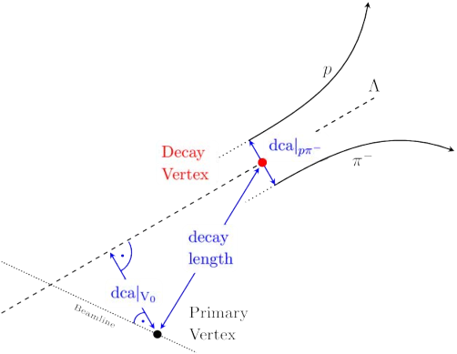
To gain access to the different effects of TOF correction the candidates sample is divided into three sub-samples: In Sub-Sample I only combinations with information for both particles are selected to check whether the algorithm works and whether the PID can be improved. In the Sub-Sample I all other cases where a TOF correction is possible are gathered to answer the question of how many candidates can be restored. The last sub-sample comprises the residual combinations which do not provide any TOF information. See Table 7.2 for further clarification. The boolean values indicate whether the specific information is available for the track or not. Note that there are cases where TOF information is available for the track but no information. This is connected to the fact that the timing information for global tracks is not reliable and therefore omitted on MicroDST level.
| 1 1 | 1 1 | Sub-Sample I |
| 1 0 | 1 0 & 1 1 | Sub-Sample II |
| 0 1 | 0 1 & 1 1 | |
| 0 0 | 1 0 & 0 1 & 1 1 | |
| 0 0 | 0 0 | Sub-Sample III |

Figure 7.3 shows a comparison of mass distributions for protons
steming from decays. For the sample with
available information for each decay track, distributions
are plotted with (blue) and without (black) applied TOF correction. A scaled
mass distribution (green) for a background-free sample
(inlet) is shown as well. The cut applied on the p invariant
mass is 1.113 - 1.118 GeV/c. Solid lines represent Gaussian functions fitted
in the range . Resulting parameters are
given in corresponding colors. Red dashed lines indicate the applied mass cuts
for particle identification. The percentages given in this and the following
figures are based on the total initial number of combinations. No differentiation has been made regarding the changing momentum
resolution. As its main feature the TOF correction algorithm changes the mass
distributions with respect to the origin of the particle: the distribution of
protons which do not fit the specific decay topology are shifted to lower
masses and broadened - see the shoulder of the blue distribution. Whereas
true protons stay at their original mass. This can be proven by generating a
background-free sample using tighter and additional cuts
- see inlet in Figure 7.3. The Gaussian function fitted to the
resulting scaled mass distribution is not shifted and its extrapolation does
not reveal any underlying or broadened structure. Applying a cut on the squared
proton mass inreases the separation power of - and non-
-daughters.

The pion mass distributions after the proton mass cut are shown in
Figure 7.4 using identical color code. The aforementioned cut on
the proton mass is already applied. Here the non-
-daughters can only be seen as tails at the lower mass end
of the pion distribution not allowing a separation as clear as for protons.
However more important, the mean pion mass is shifted by 3 MeV/c to its
nominal mass. Thus, using the TOF correction algorithm accounts for the
systematically off pion mass intrinsically.
Figure 7.5 compares the invariant mass spectra with (blue) and without (black) applied TOF correction algorithm. The distributions are fitted with Breit-Wigner + higher order polynomial functions (solid). There are two major improvements to be emphasized:

- •
The number of reconstructed ’s stays constant which proves that mainly non- -daughters have been rejected by the new proton and pion particle identification.
- •
The signal-to-background ratio improves by more than a factor 3. A comparable effect can be seen for the case of incomplete TOF information. This nicely shows the background rejection power of the algorithm for the cases of TOF information being available.
Unfortunately, the current sub-sample only covers 8% of the total number of
candidates. The residual sub-samples therefore dominate
the signal-to-background ratio with respect to the overall achievable
improvements.
Figure 7.6 shows the mass distributions for sub-sample II with (blue) and without (black) applied TOF correction. Red dashed lines indicate the mass cuts used for particle identification. In general, the distributions for both particles indicate the same features as discussed in the previous section, i.e. non-decay-daughter separation and pion pole mass shift. However, in addition a gain of 35% can be observed for the pions in a range around the respective mean masses. These are pions whose time-of-flight was intrinsically reconstructed by the algorithm using the matched TOF hit but which originally did not have a information associated (see Table 7.2). For this sub-sample, particle identification cuts on the proton and pion mass have been applied as well (indicated by red dashed lines in Figure 7.6).


The comparison of the resulting invariant mass
distributions is shown in Figure 7.7. Even for the current
statistically dominant sub-sample (60%) a significant improvement (factor 2.3)
in signal-to-background ratio can be observed suffering only a small signal
loss. Latter could mainly be caused by the fact that the applied mass cuts have
rather been chosen in favor of the uncorrected distributions.
The final invariant mass spectrum is shown in Figure 7.8. The corrected spectrum shows a slightly smaller width and a non-significant decrease of 10% in the number of s.

Regarding the signal-to-background ratio an overall
improvement of approx. 40% is achieved. The comparably lower gain in contrast
to Sub-Sample I and Sub-Sample II is due to the poor
signal-to-background ratio of the sub-sample in which no TOF correction is
possible at all. Nevertheless these improvements show the importance of
applying a TOF correction to the tracks of V decay particles regarding
background suppression.
In addition to the preceding analysis the TOF correction algorithm was applied to the decay . The corresponding plots can be found in Figure 7.9. Applying a TOF correction results in an increase of signal-to-noise ratio by a factor of 1.5 in this case.

In general, the class is supposed to be initiated once by calling its constructor. The member functions setVectors3D, setMotherTracks and correctBeta are afterwards used multiple times for the TOF correction of each decay particle. Hence, these member functions have to be invoked for each combination of daughter particles in the following order. Remember to call these functions each time as a block.
- setVectors3D(v0)(v1)...(vn)(vtof)
-
This function sets all the space vectors needed for TOF correction. The function arguments v0…vtof are all of type StThreeVectorD and define the vectors to the following space points.
- •
v0: event vertex / primary vertex
- •
v1…vn: vertices in decay chain resulting in the final particle to be corrected
- •
vtof: TOF hit
Special care has to be taken of the vectors’ ordering: Start with the event vertex and add the vertex vectors as you follow the decay chain to the final particle and its TOF hit. The final argument of setVectors3D always corresponds to the TOF hit vector.
The event vertex does not change on a candidate-by-candidate basis, of course. Nonetheless, it is given to setVectors3D as an argument to simplify the implementation and to minimize the functions to be called by the user. Make sure to start TOF correction only if a TOF hit for the particle exists! Carefully check the original time-of-flights given as an argument to the correctBeta function!
The operator () is overloaded to allow for a variable number of arguments to be given to the function and pack them into an inline container sequentially. Thus, make sure to put each function argument inside brackets as indicated in above.
Starting gcc 4.3 the so called variadic templates were included in the compiler. These function templates accept a variable number of arguments (parameter rack) which can be accessed and unpacked via the ellipsis (…) operator. This approach would have been a more elegant way to implement the class. Unfortunately, variadic templates will only be understood within the new C++0x standard which presumably will be published at the end of 2011. - •
- setMotherTracks(t0)...(tn-1)
-
Call this function to set the reconstructed 4-momentum vectors t0…tn-1 of type StLorentzVector for all mother particles. Keep the warning in setVectors3D in mind!
The number of arguments given should be smaller by 2 compared to setVectors3D. If not, the code compiles nevertheless but results in an error message during runtime. - correctBeta(helix,tof,betacorr)
-
This is the main function of the class. It takes the helix of type StPhysicalHelixD and the original time-of-flight tof of the particle to be TOF corrected and writes the corrected particle velocity into betacorr. The variable betacorr can afterwards be used to calculate a new particle mass and utilize it for particle identification. Alternatively, correctBeta can be called as correctBeta(helix,tof,betacorr,p,enum) with p the particle’s momentum and enum the particle species. In this form a default hardcoded m-cut is applied to the particle’s mass and the result returned as boolean value (enum definition: 0 = pi, 1 = K, 2 = p).
- clearContainers()
-
This function needs to be called to clear all inline containers before TOF correcting the next particle. To assure the filling of a clean container, allocated memory and pointers are deleted in this function. It could be done automatically after the TOF correction is finished. However, the user is encouraged to do it manually to have a more memorizable and controllable block of functions.
7.2 StBadRdosDb: Database Interface for TPC missing RDOs
The class StBadRdosDb has been developed to use information about the TPC’s
number of missing read-out boards (RDO) during a physics analysis. The data
taken in runs 10 & 11 are divided into run ranges with equal number of
missing RDOs and the result stored in a custom database format. StBadRdosDb can then be used to acquire the current run range given a specific run id. This
is especially helpful for analyses which rely on stable detector conditions
throughout a beam time and thus are sensitive to a run-range-dependent
efficiency correction. Upon request by STAR’s physics working group for bulk
correlations, StBadRdosDb has been announced to the collaboration
[26] and made available in the STAR CVS
[27] as well as the author’s code repository
[215]. The makeRunList.pl script used to generate official
STAR run lists for each beam time and available in a common area of STAR
scripts [216] has been modified to query the central STAR database
for the number of missing RDOs per subsequent run and the according TPC sectors
and RDO id’s. It has been extended to deal with 2010 as well as 2011 data. The
queried dataset is reduced to the list of run id’s at which the number of
missing RDOs changes. Given the correct trigger setup name and year the
genBadRdosDb.pl script is executed as
$ perl genBadRdosDb.pl AuAu39_production 2011
See the RunLog browser [217] for information on the
trigger setup name. For convenience, the code repository contains a bash script
to (re-)generate all database files: database/genAll.sh. If database files
for upcoming beam energies are generated one should make sure that the trigger
selection in the genBadRdosDb.pl script covers all runs needed in the
respective data analysis. The StBadRdosDb class does not require any STAR
libraries to be loaded and solely relies on ROOT. It provides the following
member functions to retrieve information about missing RDOs and their
respective run ranges. For their usage see the testStBadRdosDb.C ROOT macro.
- Int_t GetRunRange(Int_t runid);
-
This function is considered the main purpose of the StBadRdosDb implementation. It returns the run range index for a given run id.
- Int_t GetNrRunRanges() { return NrRanges;}
-
A helper function returning the total number of run ranges. It can be used to define arrays and histogram ranges for run-range dependent analyses.
- Int_t GetNrBadRdos(Int_t run_range);
-
An informational function returning the number of missing RDOs for a given run range.
- Int_t GetSector(Int_t run_range, Int_t nrdo);
-
GetSector returns the sector to which a specific missing RDO with index nrdo in run range run_range belongs.
- Int_t GetNrBadRdosSector(Int_t runid, Int_t sector);
-
retrieves the number of missing RDOs for a specific run id and sector.
- Int_t GetFirstId(Int_t rr) { return prun[rr];}
-
Helper function to get the first run id in the database for a specific run range.
Table 7.3 lists an examplatory database file used by the member functions of StBadRdosDb to provide information about the missing RDOs of a specific beam time. All energies for the years 2010 and 2011 have been included in the database (Section B.2). Each line in the database files indicates the start of a run range containing run id’s with equal number of missing RDOs. The second column shows the number of missing RDOs in this range followed by the according number of RDO identifiers. Each identifier encodes the missing RDO’s sector and identification number (format: sector.id). These identifiers are encoded in genBadRdosDb.pl and decoded in the class member functions GetSector and GetNrBadRdosSector.
| RunID | # bad RDOs | RDO identifiers (sector.id) |
| 11148001 | 3 | 17.01 23.02 23.08 |
| 11151010 | 4 | 11.10 17.01 23.02 23.08 |
| 11151028 | 3 | 17.01 23.02 23.08 |
| 11151040 | 4 | 17.01 21.11 23.02 23.08 |
| 11151080 | 5 | 01.07 17.01 21.11 23.02 23.08 |
| 11152053 | 6 | 01.07 07.05 17.01 21.11 23.02 23.08 |
| 11153012 | 7 | 01.07 01.09 07.05 17.01 21.11 23.02 23.08 |
| 11156032 | 8 | 01.07 01.09 07.05 09.03 17.01 21.11 23.02 23.08 |
| 11158011 | 9 | 01.07 01.09 07.05 09.03 11.01 17.01 21.11 23.02 23.08 |
7.3 StRunIdEventsDb: Database Interface for Run Id Indexing
StRunIdEventsDb has been developed to facilitate handling the run-dependent
studies for the multiple beam energies analyzed in Part I of this
thesis. The class implementation provides a mapping from a specific run id to
its corresponding index for all energies of STAR’s beam energy scan during runs
10 & 11. Moreover, the number of events can be retrieved on a run-by-run basis
for each trigger at all energies.
Analogous to Section 7.2 the perl script genRunIdEventsDb.pl is used to generate the database files. The following literal block - which also serves as configuration file for the StRunIdEventsDb class - lists all triggers for a specific combination of energy and year. Figure 7.10 shows database excerpts for 39 and 62 GeV with index, run id, and corresponding number of events per trigger. The full database and the code are available in the author’s code repository [218].
- database/config
-
7.7 2010 2 mb total11.5 2010 2 mb total19.6 2011 6 mb1-fast HLT-tracks vpd-mon bbc-small-mon-narrow zdc-mon-tac total27. 2011 5 mb1-fast vpd-mon-tac bbc-small-mon-narrow zdc-mon-tac total39. 2010 4 mb mbslow ht-11 total62.4 2010 5 min-bias min-bias-slow ht_11_mb central total200. 2010 7 Central vpd-mb NPE_18 NPE_15 NPE_11 NPEHT_25 total200. 2011 6 vpd-zdc-mb-protected NPE_18 NPE_15 NPE_11 NPE_18_ftp total

StRunIdEventsDb has been implemented as a singleton class to avoid repeated loading of the database into memory. Hence, the constructors are declared private and a public member function is added which decides on returning a pointer to a newly created instance of StRunIdEventsDb or to an already existing one. To assure singleton behavior this pointer is declared a private static member. It therefore suffices to initialize the class and load the database via
The following class member functions are implemented to communicate with the database.
- Int_t getTotalNrRunIds() { return mNrRunIds;}
-
get the total number of run id’s
- Int_t getRunIdIndex(const Int_t& runid);
-
get the index for a specific run id
- Int_t getRunId(Int_t ind);
-
get the run id for a specific index
- Int_t getNrEvents(string tn, Int_t runid);
-
get the number of events for a specific runid and trigger name
- void printAllTrigNames();
-
print all trigger names available for this energy and year
- string getTrigName(Int_t n);
-
get a single trigger name according to the index of printAllTrigNames()
Chapter 8 Transition of STAR CVS to a modern Revision Control System
The use of a revision control system to track the changes of its code basis is essential to the progress of a software development project. STAR is in no way different to other large technology companies in that many submodules exist for STAR’s detector subsystems with different people responsible for each of them. Regarding one of the largest experiments in heavy ion physics, however, there is progress made not only in terms of pure software improvements for data analyses but also an ever increasing amount of submodules needs to be added each year accompanying STAR’s detector upgrades. Still, along with the data itself, code used to process the data taken during previous beam times needs to be available to ensure reproducibility of published results and possible reproduction of DSTs when new knowledge is acquired or bugs identified. In addition, running experiments like STAR involves a myriad of custom-built tools needed for tasks such as data acquisition and backup, online monitoring and analysis, database organization and interfaces, detector alignment and calibration, track reconstruction and detector matching during data production, Monte Carlo simulations, ticket/issue submission, documentation, and publications. Hence, STAR’s code organization closely resembles the development structure and release cycles of other large software products with hierarchical work flows and a policy which requires all code to be made accessible to all collaborators. On top, most of the data analysis in STAR is conducted on multiple remote computing sites at all of which identical code deployments have to be guaranteed despite differing development environments.
All this requires maintaining a centralized revision control system like the Concurrent Versions System (CVS) [219] which currently is STAR’s system of choice. Since its beginnings, STAR has collected an immense amount of code and developed a workflow heavily centered around CVS with many tweaks to customize it. Even though other centralized successors (Subversion, for instance) have been released to overcome some of CVS’s shortcomings, STAR’s very active data taking and publication cycle have not allowed for a transition to newer systems. However, with the rise of distributed revision control systems like git [220] for instance, the many advantages of modern revision control systems do seem to make a re-evaluation of STAR’s current system necessary. Some of these advantages include instant and cheap creation and deletion of branches, branch merging and rebasing, working without connection to the remote (central) repository, significantly compressed repository sizes, fast repository cloning, temporary stashing of changes as well as selective staging and committing.
There exist many distributed revision control systems but especially git has gained traction and became very popular through the immersion of social coding and with it an increased number of open source contributions. Judging by the popularity of it, git seems to be best suited to support a developer’s workflow as it encourages frequent commits and work on parallel feature branches. Thus, likewise in STAR, collaborators seem to prefer the use of git for their private analysis code development which starts to increasingly collide with or at least inhibit the contribution to STAR’s central CVS repository. In general, due to the expensive nature of branching in CVS most of the code developed by the physicists in STAR seems to stay untracked in their home directories and unshared through the designated user areas in STAR’s CVS. It therefore seems to be time for an overhaul of STAR’s revision control system and a transition to one of the modern distributed systems.
The following two requirements need to be kept in mind, though. First, STAR’s policy requires git as a distributed revision control system to be used in a centralized but modular manner. A spread of the entire STAR software with each checkout through many home directories is unfavorable. Second, concerns about manpower almost dictate the use of already available and established open source solutions particularly because the transition would have to happen during ongoing operations. At the same time, these solutions should have a good chance of long-term support or be already stable enough for STAR not to depend on their fate.
This chapter will not discuss the merits of one revision control system over the other but give a specific suggestion on how a transition could be carried out with the best chance of going through smoothly. It is assumed that git would become the new revision control system of choice without discussing its advantages or disadvantages when compared to other distributed systems. This chapter concentrates on the execution of a transition from CVS to git by demonstrating that history conversion of all STAR CVS submodules is feasible via cvs2git and by introducing gerrit as the new review system for future code changes and gateway for all sorts of interactions with the central repository. This includes providing the necessary scripts and instructions as well as deploying an instance of the review system on a remote server for demonstration purposes. cgit is proposed as a replacement for cvsweb as web service to browse the repository.
Section 8.1 motivates and explains the proposed solution and Section 8.2 discusses a list of requirements in the framework of the proposed solution. In Section 8.3 gerrit is set up on a remote server with cgit as external browser, STAR’s CVS is converted into multiple git repositories, synchronized to the remote server and added to gerrit. Finally, Section 8.4 gives instructions on how to interact with the demonstration deployment as an end user. Note that this chapter is of special importance to STAR as it introduces a solution for modernizing its revision control system. It will serve as documentation to accompany the migration to the new system and provide references to documentation to ease the user’s transition from CVS to git.
Introductory Comment on Git for CVS Users. Git is commit based with all the rest being almost exclusively pointers. Each commit has a parent, and each branch is based on a commit. That’s why git is light in committing and branching. A tag in git, for instance, is only a pointer to a single commit and as such a direct connection to go back to a certain point in time. In general, git is fundamentally different from CVS in that its revisions are snapshots of the directory at a given point in time unlike CVS where everything is file based. Git for instance, records file renames and moves perfectly fine.
8.1 Proposed Solution: Git + Repo + Gerrit + CGit
Due to the distributed nature of git the concept of submodules is not equivalent to CVS. Submodules in CVS can be checked out and committed to separately while the minimum unit for a checkout is defined by one git repository. Submodules in git [221] are generally used for foreign libraries which evolve entirely separately but on which the software itself depends on. They are not checked out together with a git repository but need to be initialized and synchronized separately. The day-to-day usage of git submodules has some serious trip falls and is rather cumbersome which is why the community tends to avoid them. Hence, the "imitation" of a central CVS repository with git is better realized using independent git sub-repositories whose interplay is controlled via a wrapper script and a configuration file. This way multiple sub-repositories can be checked out and worked on simultaneously while global tagging and branching is maintained by the wrapper script.
Google’s Android Open Source Project (AOSP) has this issue already resolved and developed such a wrapper script in python called repo [222]. It uses a so-called manifest configuration file in xml format to organize the structural layout of the project and the remote location of the repositories as well as coordinated checkouts of specific versions. It does not replace git but operates "on top of git" [223]. AOSP’s workflow is directly applicable to STAR’s as it is general enough to serve as a template for any major collaborative software development project. AOSP’s workflow using repo is very well documented [224] and with its millions of lines of code well-proven in an heavy software development environment. These are good credentials for STAR to use it and not to fear its near-term obsolescence.
The same counts for gerrit [225], a web-based code review tool which controls all the interaction with the single git repositories including amongst others merging patches into the master branch. Gerrit achieves this control mechanism by running ssh and http daemons on two different non-standard ports. Not only does it provide a stream-lined, documented and self-sustained code review, its configuration also covers many aspects of centralized collaboration code development. For instance, it provides automated builds via the Jenkins trigger [226] and code changes will only be accepted and merged if they pass the build process and according (unit) tests. It includes email notifications, sign-offs etc. and even a REST API [227].
The standard repository browser gitweb comes with every git installation by default and can be configured to be used in gerrit. It is suggested, however, to use the cgit browser [228] instead which is more feature-rich and easily exchangeable with gitweb in gerrit. cgit is written in C and includes caching if desired, both of which make it extremely fast and very responsive. cgit is straight-forward to set up and its development is very active. In March 2013 it has been selected by the Linux Kernel as its primary repository browser [229, 230].
In a nutshell, git + repo + gerrit + cgit gives STAR the best chances to succeed in a CVS to Git migration while significantly modernizing its workflow and code review.
8.2 STAR specific Requirements and Requests
In the following a list of requirements and requests which are specific to STAR is discussed. These items have been identified as important questions to STAR through discussion with the project leader of STAR’s software & computing group, Dr. Jerome Lauret (jlauret@bnl.gov).
- Centralized Workflow with Feature and Development Branches
-
In the past, the lack of convenient use of feature and temporary branches in CVS has caused users to maintain copies of entire CVS submodules of StRoot/ in their designated user area at offline/users/. The user areas do not serve the purpose of maintaining official STAR code until it is ready to be committed into the main branch. They exist as an area for users to share code which is not STAR official but still of interest for the entire collaboration. Thus, the new system has to enable the use of development and feature branches for the user to work on while still within the central repository. Also, the new platform has to take care of the organization of these parallel branches in terms of sharing, reviewing and merging with the main branch and core development.
These concerns and appearances of "offline-branching" and inconvenient parallel development are what caused the development of git in the first place. Together with repo and gerrit as tools to organize the interplay of many git repositories as well as the parallel coding of multiple developers, the new system proposed in Section 8.1 covers all possible aspects of such a development environment in a very convenient and well documented manner. See the quick intro of gerrit for a standard "life of a patch" [225].
Moreover, even though git is of distributed nature all code committing must be encouraged to go to a central repository. This principle is enforced by STAR rules and must not be violated when switching to a new revision control system. Here again, the usage of many git repositories as a joint central entity is the main purpose for the development of gerrit by AOSP as outlined in Section 8.1. Gerrit serves as the sole gateway to the repositories and while it is possible to push directly to the git repositories behind gerrit and thus entirely circumvent the review, this is not desired and can be switched off completely. - Authentication and Authorization
-
In contrary to a publicly accessible open source project such as AOSP, strict authentication and authorization mechanisms have to be enforced in STAR. These methods have to be consistent with BNL policies. For instance, users without valid RCF account are not to be allowed write access to repositories served by the new platform.
In its default setup gerrit manages users and its logins via the OpenID mechanism. Internally users are organized in groups with specific access rights globally or on a per project basis. Gerrit provides ACL authorization like CVS does but its capabilities allow very fine grained and extensive control of the repositories and its branches (see [225]). For authentication already existing kerberos accounts can be used instead of OpenID. This is not in the scope of the demonstration deployment of this chapter as it would only be possible to implement on a dedicated server at BNL with access to krb5.keytab [231]. This needs to be explored after the user’s reception of the new system has been reviewed. Hence for simplicity, the demonstration deployment of the gerrit instance in this chapter will only be based on a single user login (protected) and multiple associated e-mail addresses and ssh-keys (see Section 8.4).
Two aspects of authentication and authorization will have to be evaluated in the future. First, having an automated mechanism to port the current CVS access rules (karma) into gerrit would be favorable to preserve access rights to repositories and branches. Second, CVS currently does not have truely public areas which are not subject to STAR’s access control. STAR might profit if such areas would be realizable with the new platform enabling STAR collaborators to participate in community work.
gitolite [232] is an alternative AA system to setup access controlled hosting of git repositories. Access on per project and per branch basis is configured via a dedicated gitolite-admin repository with a central configuration file and public ssh-keys. It integrates very well with cgit, too, and repo can still be used to organize multiple git repositories at once. Without a gerrit instance, however, repo upload is redundant, of course. Gitolite is a very good option for the hosting of git repositories with a small number of developers who organize the control of a small amount of development and feature branches themselves and do not need automated code review nor continuous build integration. Thus, to secure the long-term stability of code organization and review in STAR gerrit seems to be better suited. - Demonstration Deployment and Trial Phase
-
For the final migration to git and the associated deployment of the gerrit platform a phase of daily incremental conversion of CVS to git history would not necessarily be required. During a trial phase with a gerrit demonstration deployment — as is the goal of this chapter — CVS and git could run in parallel and even diverge. The demonstration deployment of this chapter will already put in place a full conversion of STAR’s CVS repository for users to play with. In addition, it shall encourage the involvement of the people responsible for each repository to thoroughly check their converted history. This should help in identifying failed conversions of single commits as well as possible merging or splitting of historically linked CVS submodules into git repositories. Following this feedback, these requests can be scripted into the automated conversion (see Section 8.3) before a date is scheduled for the final migration at which the STAR’s CVS repository is retired for good.
- Repository Browser
-
The core of STAR’s developer team is long-time used to the cvsweb experience of browsing code and its history. The proposed repository browser cgit already provides a large set of features and comes very close to the conception of browsing code in STAR. Contrary to STAR’s CVS, the new system will not have the entire STAR CVS repository and all its submodules mangled into one big git repository but split them up into many smaller ones organized by the repo script. Thus, the cgit browser will serve these repositories as independent unrelated entities. It allows, however, to organize the repositories into categories which significantly facilitates the browsing. Pagination can be switched off such that the general layout of the cgit browser will look like the Linux Kernel’s [230]. CGit further features sorting the repository listing on its landing page based on name, description, owner and idle time. Together with the very fast search function, the list of repositories can quickly be reduced to the ones of interest to the user.
Still, cgit is an open source project and thus helpful features like "Expand/Collapse Categories" can be suggested to the community or contributed. As for the representation of a repository itself in cgit, functionalities present in cvsweb are mostly implemented in cgit [233], too, but will need some getting used to on the user’s side.
In the author’s opinion only GitLab [234] would be a serious alternative candidate to use as repository browser. Rather than only being a repository browser, however, it aims at being an open source alternative to the popular GitHub social coding platform [235]. Hence, it does not fit STAR’s requirements to interface with gerrit as well as cgit does.
8.3 Migration from CVS to new System
This section documents in detail the steps to be taken to first set up a gerrit instance on a remote server with cgit as an external repository browser (Section 8.3.1) and then convert the CVS submodules StRoot, kumacs, pams, StDb, StarDb, asps, QtRoot, StarVMC and mgr into git repositories (Section 8.3.2). The converted repositories will also be added to the gerrit review system.
The demonstration deployment of gerrit in this section will only rely on a simple single sign-on via HTTP authorization. The credentials are chosen to be the common ones for access to usual STAR protected areas. This allows all STAR collaborators to interact with the system with administrator priviledges given that they add their ssh-key to the STAR Protected user on gerrit as described below. However, it still restricts read access to STAR’s code to its collaborators only. This is by design such that all collaborators contributing to the STAR code repository can try out the new system before a production deployment with fine-grained access control is started.
The gerrit instance which will be set up in the following will also be used to serve all scripts and configuration files necessary for the deployment in a dedicated repository named git4star. Thus on all sites and for all users interacting with the gerrit review system a dedicated ssh-key pair has to be generated and its public key uploaded to the STAR Protected user on gerrit 11 1 http://gerrit4star.the-huck.com/#/settings/ssh-keys . This needs to be done for end users uploading changes as well as admins converting CVS repos and creating projects. The source codes for the shell scripts are also appended to this thesis in Section B.3.
Last, the following entry needs to be added for the gerrit4star host to ~/.ssh/config. After that connecting to gerrit via ssh gerrit4star should present itself with a welcome message and exit. All the subsections in this section assume that the reader can clone the git4star repository via git clone gerrit4star:git4star on all sites.
8.3.1 On the Web Server
- Assumptions
-
Gerrit runs under a dedicated gerrit4star user at the domain http://gerrit4star.the-huck.com with the external cgit browser at http://cgit4star.the-huck.com.
- Apache Configuration
-
As super-user, setup a name-based virtual host to serve cgit at http://cgit4star.the-huck.com [236] and second one with reverse proxy and HTTP authentication for the gerrit review system at http://gerrit4star.the-huck.com (see [225]). Restrict access to both by adding the STAR Protected user to htpasswd and including the appropiate section in the apache configuration. This user will later be used as single sign-on and thus administrator login to gerrit as well as for all repository interaction through ssh (see above’s ~/.ssh/config). Example cgit4star.the-huck.com and gerrit4star.the-huck.com apache configuration files are available in the git4star script repository (see following step).
- Get git4star script repository
-
As gerrit4star user, clone the git4star script directory:
git clone gerrit4star:git4star $HOME/git4star - Setup cgit browser
-
The following will clone, init, config and install cgit [237]. It will configure the cgit.cgi script to be installed in $CGIT_SCRIPT_PATH and anything else in $prefix. Adjust both in cgit.conf to reflect your web server setup.
git clone git://git.zx2c4.com/cgit $HOME/cgitcd cgit && git submodule init && git submodule update# copy cgit config filecp $HOME/git4star/cgit.conf $HOME/cgit/make -j4# switch user if ’gerrit4star’ doesn’t have sudo perms# go back to ’gerrit4star’ user afterwardssudo make install# copy cgitrc to $CGIT_CONFIG (see cgit.conf)cp $HOME/git4star/cgitrc $prefix/etc/cgitrc# go to http://cgit4star.the-huck.com to see whether cgit runs# ignore "no repositories found" message - Install gerrit
-
The code below downloads, installs and configures the HTTP proxy for gerrit [225]. The configureHttpProxy.sh script also starts the ssh and http daemons. http://cgit4star.the-huck.com should now list an AllProjects.git repository which appears to be empty and visiting http://gerrit4star.the-huck.com should now show the gerrit welcome page after logging in using the STAR protected credentials. Fill out "Full Name" as well as optionally register an e-mail and add a ssh-key.
cd $HOME # for gerrit4star userwget https://gerrit-releases.storage.googleapis.com/gerrit-2.6.1.war# the following batch install will raise a FAILED notice but that’s okjava -jar gerrit-2.6.1.war init --batch -d $HOME/gerrit_review~/git4star/configureHttpProxy.sh - Configure CGit as external browser
-
Gerrit will still show links to its internally handle gitweb browser. Running $HOME/git4star/configureCGit.sh configures cgit as external browser instead of gitweb. For the final $HOME/gerrit_review/etc/gerrit.config see the $HOME/git4star/gerrit.config file in the git4star script repository. Check the cgit links for AllProjects.git in gerrit after configuration to confirm a correct configuration.
- Final Step
-
Set additional access rights "Create Reference" and "Push Merge Commit" for administrators under refs/* at http://gerrit4star.the-huck.com/#/admin/projects/All-Projects,access. This is later needed to push the newly converted CVS repositories directly into gerrit.
8.3.2 In a Working Directory at BNL with CVSROOT Access
- Assumptions
-
All of the following code will be executed within a dedicated working directory. Access to the git4star script repository is assumed as well.
<WORKDIR> = /star/institutions/lbl/huck/star_cvs2git/ - Convert STAR CVS
-
The following code downloads and unpacks cvs2git [238]. The CVS submodules StRoot, kumacs, pams, StDb, StarDb, asps, QtRoot, StarVMC and mgr are then converted to git via the convertStarCVS.sh script. Make sure to check the environment variables in this script before executing it!
cd <WORKDIR> && git clone gerrit4star:git4starwget http://cvs2svn.tigris.org/files/documents/1462/49237/cvs2svn-2.4.0.tar.gztar -xvzf cvs2svn-2.4.0.tar.gzcd git4star# the following converts all repos and takes about 1.5h!./convertStarCVS.sh | tee cvs2git.logTwo remarks on the conversion of CVS to git. First, the conversion of STAR’s CVS repository to git for production deployment of gerrit would require a list of all CVS committers in the format username : Full Name <E-Mail> to be fed into the conversion. This list would map usernames to the format in which git uses them because each git commit requires the committer to provide an e-mail address, too. This is due to the principle that committers should minimally be reachable by e-mail. Such a list could be either generated by using the finger command or direct access to a database at BNL providing this information. Second, a general freely choosable "cvs2git" user including name and e-mail would need to be provided during the conversion. This user gets used for commits for which CVS does not record the original author. More information about these details can be found in the my.cvs2git.options file in the git4star script repository.
- Create and upload Gerrit Projects
-
Running createGerritProjects.sh in $workdir/git4star creates all projects in gerrit and pushes the according repositories to gerrit. The script also adds sign-off and change-id requirements to all projects in gerrit.
- Write Manifest for repo
-
When executing the writeManifest.sh script a default manifest named default.xml is generated based on the converted CVS repositories which can later be used to initialize the STAR repository for the use with the repo script (see Section 8.4).
| git (MB) | CVS (MB) | |
| StRoot | 363 | 480 |
| kumacs | 14.8 | 1.74 |
| pams | 37.6 | 128 |
| StDb | 6.47 | 4.58 |
| StarDb | 199 | 576 |
| asps | 16.1 | 47.5 |
| QtRoot | 16.3 | 12.5 |
| StarVMC | 47.5 | 116 |
| mgr | 4.66 | 5.93 |
| total | 705 | 1373 |
8.4 End User Instructions for Gerrit Demonstration Deployment
- Setup Gerrit Access
-
Add ssh-key to STAR Protected user in gerrit as describe in the introduction part of this section. Run ssh gerrit4star to check whether you see the welcome message and thus are able to connect to gerrit correctly. Add your git-config e-mail address to the STAR Protected user at http://gerrit4star.the-huck.com/#/settings/contact and confirm it via the link in the e-mail sent to you. Put the following into your ~/.gitconfig.
- Setup, init and start sync’ing with repo
-
First install the repo script as described in [239]. A good introduction and overview of the usage of repo and the associated workflow can be found in [240, 241]. To get started, create an empty directory to hold your working files.
mkdir MyStarProjects && cd MyStarProjectsThe manifest specifies where the various repositories included in the STAR repository will be placed within your working directory. Init your working directory using the default.xml in the git4star script repository:
repo init -u gerrit4star:git4star --config-nameWhen prompted, configure repo with your full name and the email you added above to the STAR Protected user in gerrit. ALL projects can be pulled down to your working directory as specified in the default manifest by running a simple repo sync. However, this is not desired in most cases. The repo script allows for only a list of gerrit projects to be synchronized via
repo sync StRoot-StAnalysisMaker StRoot-StHbtMaker - Start Work and Upload Changes for Review
-
The workflow of repo together with gerrit is very well documented in [242, 243]. Start a new development branch in all the repos you sync’ed via
repo start <branchname> --allChange to the git repository of your choice, start playing around, change files and when you are done, commit everything via
git commit -a -s -m "commit message"Add your ssh-key to the ssh-agent (ssh-add ~/.ssh/<ssh-key-name>) and upload your changes to gerrit for review via a simple
repo uploadCheck repo help for more. Screenshots of Gerrit and CGit for STAR are appended in Section B.4.
Chapter 9 Open Source Contribution of Physics Analysis and Documentation Tools
9.1 ckon: Automatic Build Tool for ROOT Analyses
ROOT [163] allows for the automatic compilation of shared libraries using the ACLiC compiler [244]. This is very convenient for the quick use of compiled libraries in CINT but the organization of code developed for a physics analysis project would be cumbersome regarding its size and the resulting intra-project library dependencies. On top, ROOT-based shared libraries are mostly invoked through a macro and not a compiled program. The latter significantly improves the quality of a software project. Most bugs are detectable during compilation and not runtime and run control can be extended through command line options and arguments. This avoids constant recompilation due to hard-coding of I/O variables, for instance, and facilitates the use in shell scripts. Writing Makefiles for each library and program on the other hand is a difficult, time-consuming and repetitive task. This section is dedicated to a comprehensive solution of this issue.
On all computing sites STAR provides the user with the perl script cons to automatically compile shared libraries which rely on ROOT as well as StRoot software. However, cons is somewhat outdated and does not provide flexible configuration options. It covers a standard source code layout in which each subdirectory of StRoot is compiled into a library. For custom configuration like deeper structures which would need cons to recursively scan directories, for instance, the user needs to modify the cons script itself. Moreover, it is not straight-forward to set up on a local machine when StRoot software is not even needed. The author hence uses Autoconf and its simplified Makefile-"language" to automatically generate Makefiles specific to the underlying operating system. Autoconf is well established amongst software looking to be platform independent and provides GNU’s known "configure / make / make install" workflow including distribution package management ("make clean / make distclean / make dist").
This is a first step towards an easy-to-maintain project layout but still requires the setup of Automake-Makefiles with library-specific naming conventions. This task is already stream-lined when compared to manually writing Makefiles but still is error-prone and very repetitive. The latter, however, makes the entire process wrapable into the dedicated software tool ckon. On top of relieving the user from any duty to write Makefiles at all, this tool makes it easy to include foreign code or third-party libraries as well as the user’s own core utility and database classes based on a simple project-specific YAML configuration file. All which is needed to build an entire project is ckon setup && ckon with the user deciding on the source directory’s layout.
The following first outlines the usage of GNU’s autoconf in conjunction with
ROOT which is based on a talk given by the author at the Junior’s Day of the
STAR Collaboration Meeting in November 2011 at LBNL. Find the talk titled "An
example-driven introduction to using autoconf/automake (& Doxygen) for the
organization of C++ data analysis software within the CERN ROOT framework"
published on speakerdeck.com [28]. The automatic build tool
ckon is subsequently introduced which was developed by the author to automate
the suggested autoconf-based workflow for ROOT. Even though doxygen support is
discussed in the presentation the reader is referred to Section 9.3 in which the
author opts for Asciidoc to cover documentation of a physics analysis project.
The listing below demonstrates a possible layout for a simple ROOT analysis using Autoconf. The according source code is published at [245]. For references, see [246-251].
-
configure.ac required for ./configure script
-
Automake-Makefile for generating the main program bin/runhSimple
-
source code for main program to control the class behavior.
decodes options and re-initializes argc/argv for TRint -
hSimple class based on $ROOTSYS/tutorials/hsimple.C [252]
-
same for Options class [253].
for demonstration purposes only (better use Boost’s program_options) -
install program in bin/ and run it:
autoreconf -v --force --install && ./configure && makerunhSimple "out/hsimple.root"runhSimple -N 1000000 "out/hsimple.root"runhSimple -O "pics/test.png" "out/hsimple.root"runhSimple -N 20000 -O "pics/test.png" "out/hsimple.root" -
build & package distribution management
make dist # generate tarballmake clean # remove build filesmake distclean # remove everything generated by automake
ckon is a C++ build tool which automatically takes care of compilation, dictionary generation and linking of programs and libraries developed for data analyses within the CERN ROOT analysis framework [163]. Given a source directory it recursively parses header include statements to figure out which libraries the main programs need to be linked to. It uses automake/autoconf [254] to be platform independent and GNU install compliant. In addition, m4 macros [255] are automatically downloaded and the according compiler flags included based on a list of boost [256] libraries provided in the config file. For the purpose of YAML database usage, a m4 macro can be downloaded during setup to link against the yaml-cpp library [257]. The project’s source code has been published on github [258] with the according documentation at [259]. It was written by the author of this thesis with invaluable contributions by Hiroshi Masui. It is released under the MIT License [260] and requires the following list of software already installed on the system: m4/1.4.6, autoconf/2.68, automake/1.11.4, libtool/2.4, boost/1.50, libcurl/7.27.0. Install ckon via
Shown below are the generic command line options which can be given to ckon. The long option --ckon_cmd is implemented as optional positional option to run the setup, clean all compilation products (i.e. make clean) and globally install libraries and programs (i.e. make install).
Run ckon setup to generate the files configure.ac and .autom4te.cfg (both
autoconf specific with no need for modifications) as well as ckon.cfg.
Modify the latter to resemble your directory structure and linker options.
Simply remove the lines/options you do not need, thus using the default
options.
The following options can be set on the command line or preferably in
ckon.cfg. Optionally, a file named ckonignore with a list of strings to be
ignored during the build process, can be created in the working directory.
Wildcards are not supported (yet). Instead, each path currently processed by
ckon will be checked against the strings/lines in ckonignore. If one of the
strings in ckonignore is contained in the currently scanned path, the path is
ignored/skipped.
In addition, unregistered options of the form ldadd.prog_name are allowed to use for adding LDFLAGS to the linker of specific programs. The given string/value is added verbatim in LDADD. Unregistered options are only allowed in ckon.cfg. For instance, link the programs genCharmContrib and dedxCut versus Pythia6 [261] and RooFit [177] by adding the following to ckon.cfg.
ckon.boost is set during ckon setup to use and link against specific boost
libraries. Try not to run rootcint (ckon.NoRootCint) on the library if
compilation fails.
Since version 0.4 ckon allows for the automatic download
of a yaml.m4 macro during ckon setup to link against the yaml-cpp library
[257]. Please submit an issue [262] if the macro does not
find the yaml-cpp library after you installed it. This added functionality
should not break anything if you choose not to use YAML during ckon setup.
For the recursive header scan to work, make sure that all include directives
for C++ and ROOT headers are enclosed in <...>! Only your local/private
headers should be enclosed in "...". Otherwise ckon will fail reporting a
basic_string::_S_create error.
Put header and source files for each library into a separate folder in
ckon.src_dir. Running ckon should automagically take the right action for
the current status of your build directory (no need to run ckon clean before
re-compilation). Makefiles and LinkDef’s are generated automatically based on
the contents and timestamps in the ckon.src_dir directory. A typical
directory structure is shown in Section B.5 using the current defaults for
illustration purposes.
9.2 ccsgp: Publication-ready Plots with Gnuplot and Python
ccsgp [263] is a plotting library based on gnuplot-py which wraps the necessary calls to gnuplot-py into one function called make_plot. The keyword arguments to make_plot provide easy control over the plot-by-plot dependent options while reasonable defaults for legend, grid, borders, font sizes, terminal etc. are handled internally. By providing the data in a default and reasonable format, the user does not need to deal with the details of "gnuplot’ing" nor the internals of the gnuplot-py interface library. Every call of make_plot dumps an ascii representation of the plot in the terminal and generates the eps hardcopy original. The eps figure is also converted automatically into pdf, png and jpg formats for easy inclusion in presentations and papers. In addition, the user can decide to save the data contained in each image into hdf5 files for easy access via numpy. The function repeat_plot allows the user replot a specific graph with different properties, like axis ranges for instance. The make_panel user function facilitates plotting of 1D- or 2D-panel images with merged axes. The library allows for the generation of identical plots independent of the data input source (ROOT, YAML, ascii, pickle, hdf5, etc.) using the full power of python. The name ccsgp stands for Carbon Capture and Sequestration GnuPlot as this library started off in the context of CCS research [264]. The package ccsgp_get_started [265, 266] provides a sample setup to get started with ccsgp. ccsgp is initialized as a module and its usage demonstrated with dedicated functions in the examples module. Helpful utility functions are also included to complement the features of ccsgp. Installation and implementation details for both, ccsgp and ccsgp_get_started, are appended in Section B.6.
9.3 wp-pdf: Setup/Tools for Physics Analysis Homepage and Note
During the STAR review process of physics analyses for publication detailed
reports have to be provided to the committee in form of a homepage as well as
in pdf-format. Usually, this means twice the workload for presenting the same
content. The markup language AsciiDoc and the python script blogpost both
developed by S. Rackham are the ideal tools to separate writing and compiling
information from its presentational form [267]. The content only
exists in text files which are pushed to a Wordpress instance for display in
html or which can be converted into a docbook [268] to generate an
analysis note. The a2x tool-chain takes care of this process [269].
Text-based source files also make it possible to track progress and changes
with a revision control system. This approach significantly reduces the
workload while at the same time improves the quality of the analysis note
and corresponding homepage by using the tools optimized for the respective task.
In this section the collection of commands required to achieve this goal is condensed into a small Makefile providing descriptive targets. This makes it very convenient to update WordPress pages from the command line as well as create the corresponding pdf versions. The instructions are tuned to the usage of the Wordpress instance in the context of a high energy physics analysis.
wp-pdf has been announced on Asciidoc’s mailing list [270] and a public demonstration page which uses the AsciiDoc userguide itself has been deployed at http://asciidoc.the-huck.com. The following instructions and the Makefile are also published on github [271]. On a side note, images can quite comfortably be organized and served remotely 11 1 see http://downloads.the-huck.com by using git-annex [272, 273].
- setup wordpress
-
- •
configure apache [236]
- •
create mysql database [274]
- •
install Wordpress [275]
- •
add upgrade constants to wp-config.php [276] (see Section B.7)
- •
change to www-data owner: sudo chown -R www-data:www-data public/
- •
install Foghorn theme, adjust Appearance Theme Options
- •
install the following wordpress plugins:
Options Framework, Disable Comments, CMS Page Order, Multi-level Navigation Plugin, WP Google Fonts (font: Gentium Book Basic), WP PHP widget, MathJax-Latex (change options: Force Load, Use wp-latex syntax?, Use MathJax CDN?) - •
set up Sidebar in Appearance Widgets:
Search, Section Index, PHP Widget (see Section B.7) - •
go to Settings Permalinks and use post name as URL
- •
after pushing front page, go to Settings Reading and choose it as static front page
- •
- install blogpost
-
The official README and source code of blogpost can be found at [277, 278]. The author of this thesis implemented two changes on top of blogpost version 0.9.5: First, allow more than the 10 last most recent posts/pages to show up in info and second, a bugfix for inline-latex via the config macro [279]. This customized version is available on github [280] along with install instructions in its README file.
- prepare for deployment
-
In the working directory adjust docinfo.xml. If you will be including images, create a symbolic link named images linking to the image directory and/or adjust Makefile (see Section B.7).
- use Makefile for hp, pdf & latex
-
Let wp-pdf do the "magic":
After publishing a page for the first time, use Pages Page Order to arrange pages.
9.4 rmrg: Automization Class and Program for ROOTs hadd
rmrg is a command line program to merge ROOT Trees and Histograms with additional features and increased control currently missing in ROOT’s hadd [29]. Primarily,
- •
automatic file-list generation based on an input directory scan
- •
step-by-step verbose TTree and Histogram merging
- •
options for number of files to merge at once and minimum file size
This tool was developed to be included as afterburner in the PicoDst production at LBNL. Small output files would be merged on a run-by-run basis which provides a homogenous landscape of input files to relieve the queueing systems of the batch farms. The code is published on github [281].
Part III Appendix
Chapter 10 Bibliography
- 1.
D. Gross and F. Wilczek. A watershed: the emergence of Quantum-Chromo-Dynamics. CERN Courier. http://cerncourier.com/cws/article/cern/52034
- 2.
K.A. Olive et al. (Particle Data Group). Review of Particle Physics. Chin. Phys. C38, 090001. https://doi.org/10.1088/1674-1137/38/9/090001
- 3.
R. Rapp and J. Wambach. Chiral symmetry restoration and dileptons in relativistic heavy ion collisions. Adv. Nucl. Phys. 25, 1. http://arxiv.org/abs/hep-ph/9909229
- 4.
E. Shuryak. Quantum-Chromo-Dynamics and the theory of superdense matter. Physics Reports 61, 71–158. https://doi.org/10.1016/0370-1573(80)90105-2
- 5.
National Science Foundation et al. 1975. Report of the Workshop on BeV/Nucleon Collisions of Heavy Ions - How and Why. Bear Mountain, NY.
- 6.
H.G. Baumgardt et al. Shock waves and mach cones in fast nucleus-nucleus collisions. Zeitschrift für Physik A273, 359–371. https://doi.org/10.1007/BF01435578
- 7.
U. Heinz and G. Kestin. Jozso’s Legacy: Chemical and Kinetic Freeze-out in Heavy-Ion Collisions. EPJ 155, 75. https://arxiv.org/abs/0709.3366
- 8.
J.-Y. Ollitrault. Anisotropy as a signature of transverse collective flow. PRD 46, 229–245. https://doi.org/10.1103/PhysRevD.46.229
- 9.
A. Poskanzer and S. Voloshin. Methods for analyzing anisotropic flow in relativistic nuclear collisions. PRC 58, 1671. https://arxiv.org/abs/nucl-ex/9805001
- 10.
G. David, R. Rapp, and Z. Xu. Electromagnetic Probes at RHIC-II. Phys.Rept. 462, 176–217. https://arxiv.org/abs/nucl-ex/0611009
- 11.
R. Rapp. Update on SR in the Context of Dilepton Data. J.Phys.Conf.Ser. 420, 012017. https://arxiv.org/abs/1210.3660
- 12.
A. Drees. Dileptons and photons at RHIC energies. Nuclear Physics A830, 435c–442c. https://doi.org/10.1016/j.nuclphysa.2009.10.036
- 13.
CERES Collaboration. Enhanced Production of Low-Mass e+e- in 200 GeV/N S-Au at CERN SPS. PRL 75, 1272. https://doi.org/10.1103/PhysRevLett.75.1272
- 14.
NA60 Collaboration. First measurement of the SF in high-energy N+N. PRL 96, 162302. http://arxiv.org/abs/nucl-ex/0605007
- 15.
PHENIX Collaboration. Measurement of e+e- continuum in pp/AuAu at 200 GeV and implications for direct production. PRC 81, 034911. http://arxiv.org/abs/0912.0244
- 16.
STAR Collaboration. Dielectron mass spectra in Au+Au at 200 GeV. PRL 113, 022301. http://arxiv.org/abs/1312.7397
- 17.
HADES Collaboration. Dielectron production in C+C collisions at 2-AGeV. PRL 98, 052302. https://arxiv.org/abs/nucl-ex/0608031
- 18.
HADES Collaboration. Study of dielectron production in collisions at 1A-GeV. PLB 663, 43. https://doi.org/10.1016/j.physletb.2008.03.062
- 19.
STAR Collaboration. Mid-rapidity e+e- spectrum in p+p at 200 GeV. PRC 86, 024906. https://doi.org/10.1103/PhysRevC.86.024906
- 20.
STAR Collaboration. Experimental Exploration of QCD Phase Diagram: Search for Critical Point and Onset of Deconfinement. http://arxiv.org/abs/1007.2613
- 21.
W. Cassing et al. Excitation functions of hadronic observables from SIS to RHIC energies. NPA 674, 249. http://arxiv.org/abs/nucl-th/0001024
- 22.
O. Linnyk. 2014. Private Communication.
- 23.
STAR Collaboration. STAR Public Note 0598: Studying the phase diagram of QCD matter at RHIC. https://drupal.star.bnl.gov/STAR/starnotes/public/sn0598
- 24.
StBTofUtil. www.star.bnl.gov/cgi-bin/protected/cvsweb.cgi/StRoot/StBTofUtil
- 25.
- 26.
- 27.
P. Huck. www.star.bnl.gov/cgi-bin/protected/cvsweb.cgi/offline/users/huck
- 28.
- 29.
- 30.
D. Gross and F. Wilczek. Ultraviolet Behavior of Non-Abelian Gauge Theories. PRL 30, 1343. https://doi.org/10.1103/PhysRevLett.30.1343
- 31.
H. Politzer. Reliable Perturbative Results for Strong Interactions? PRL 30, 1346–1349. http://doi.org/10.1103/PhysRevLett.30.1346
- 32.
D. Gross and F. Wilczek. Asymptotically Free Gauge Theories I. Phys. Rev. D8, 3633. https://doi.org/10.1103/PhysRevD.8.3633
- 33.
D. Gross and F. Wilczek. Asymptotically Free Gauge Theories II. Phys. Rev. D9, 980. https://doi.org/10.1103/PhysRevD.9.980
- 34.
H. Georgi and H. Politzer. Electroproduction scaling in asymptotically free theory of strong interactions. PRD 9, 416. https://doi.org/10.1103/PhysRevD.9.416
- 35.
S. Bethke. World summary of the strong coupling constant. Nucl.Phys.Proc.Suppl. 234, 229–234. https://arxiv.org/abs/1210.0325
- 36.
G.F. Sterman. QCD and jets. http://arxiv.org/abs/hep-ph/0412013
- 37.
M. Peskin and D. Schroeder. An Introduction To Quantum Field Theory. Westview Press.
- 38.
P. Petreczky. Lattice QCD at T0. J.Phys. G39, 093002. https://arxiv.org/abs/1203.5320
- 39.
K. Liu. Finite Baryon Density Algorithm. http://arxiv.org/abs/hep-lat/0312027
- 40.
M. Gyulassy and L. McLerran. New forms of QCD matter discovered at RHIC. NPA 750, 30. https://arxiv.org/abs/nucl-th/0405013
- 41.
G. Baym. Relativistic Heavy Ion Collider: From dreams to beams in two decades. NPA 698, 23–32. https://arxiv.org/abs/hep-ph/0104138
- 42.
I. Arsene et al. Quark–gluon plasma and color glass condensate at RHIC? The BRAHMS perspective. NPA 757, 1. https://doi.org/10.1016/j.nuclphysa.2005.02.130
- 43.
B. Back et al. The PHOBOS perspective on discoveries at RHIC. Nucl. Phys. A757, 28–101. https://doi.org/10.1016/j.nuclphysa.2005.03.084
- 44.
J. Adams et al. Experimental and theoretical challenges in the search for the quark–gluon plasma: The STAR Collaboration’s critical assessment of the evidence from RHIC collisions. NPA 757, 102. https://doi.org/10.1016/j.nuclphysa.2005.03.085
- 45.
K. Adcox et al. Formation of dense partonic matter in relativistic nucleus–nucleus collisions at RHIC: Experimental evaluation by the PHENIX Collaboration. NPA 757, 184–283. https://doi.org/10.1016/j.nuclphysa.2005.03.086
- 46.
L. Cifarelli, L.P. Csernai, and H. Stöcker. The Quark-Gluon Plasma, a nearly perfect fluid. Europhys. News 43, 29–31. https://doi.org/10.1051/epn/2012206
- 47.
QM 11. JPG 38. http://iopscience.iop.org/0954-3899/38/12
- 48.
QM 12. NPA 904. https://doi.org/10.1016/S0375-9474(13)00372-2
- 49.
QM 14. NPA 931. www.sciencedirect.com/science/journal/03759474/931
- 50.
F. Karsch. Lattice QCD at high temperature and density. Lect. Notes Phys. 583, 209–249. https://arxiv.org/abs/hep-lat/0106019
- 51.
I. Bombaci. Quark deconfinement in neutron stars and -ray bursts. J.Phys.Conf.Ser. 50, 208. https://doi.org/10.1088/1742-6596/50/1/024
- 52.
R. Hagedorn. New derivation of the statistical theory of particle production with numerical results for p-p at 25 GeV. Nuovo Cimento 15, 434. http://doi.org/10.1007/BF02902578
- 53.
S. Gupta et al. Scale for the Phase Diagram of Quantum Chromodynamics. Science 332, 1525. https://doi.org/10.1126/science.1204621
- 54.
T. Bhattacharya et al. QCD Phase Transition with Chiral Quarks and Phys. Quark Masses. PRL 113, 082001. https://doi.org/10.1103/PhysRevLett.113.082001
- 55.
Y. Nambu and G. Jona-Lasinio. Dynamical Model of Elementary Particles Based on Superconductivity I. Phys. Rev. 122, 345. https://doi.org/10.1103/PhysRev.122.345
- 56.
Y. Nambu and G. Jona-Lasinio. Dynamical Model of Elementary Particles Based on Superconductivity II. Phys. Rev. 124, 246. https://doi.org/10.1103/PhysRev.124.246
- 57.
T. Muta. Foundations of Quantum Chromodynamics. An Introduction to Perturbative Methods in Gauge Theories. World Scientific Lecture Notes in Physics.
- 58.
D. Gross et al. QCD and instantons at finite temperature. Reviews of Modern Physics 53, 43. https://doi.org/10.1103/RevModPhys.53.43
- 59.
R.D. Pisarski and F. Wilczek. Remarks on the chiral phase transition in QCD. PRD 29, 338–341. https://doi.org/10.1103/PhysRevD.29.338
- 60.
A. Masayuki and Y. Koichi. Chiral restoration at finite density/temperature. NPA 504, 668. https://doi.org/10.1016/0375-9474(89)90002-X
- 61.
K. Fukushima and T. Hatsuda. Phase diagram of dense QCD. Rept.Prog.Phys. 74, 014001. https://arxiv.org/abs/1005.4814
- 62.
T. DeGrand et al. Masses and other parameters of the light hadrons. PRD 12, 2060–2076. https://doi.org/10.1103/PhysRevD.12.2060
- 63.
H. Satz. Deconf./percolation. NPA 642, 130. https://arxiv.org/abs/hep-ph/9805418
- 64.
E. Shuryak. Two scales and phase transitions in Quantum-Chromo-Dynamics. PLB 107, 103–105. https://doi.org/10.1016/0370-2693(81)91158-8
- 65.
Y. Aoki et al. The QCD transition temperature: Results with physical masses in the continuum limit. PLB 643, 46. https://arxiv.org/abs/hep-lat/0609068
- 66.
K. Fukushima and C. Sasaki. The phase diagram of nuclear/quark matter at high baryon density. Prog.Part.Nucl.Phys. 72, 99. https://arxiv.org/abs/1301.6377
- 67.
T. D. Lee and G. C. Wick. Vacuum stability and excitation in a spin-0 field theory. PRD 9, 2291. https://doi.org/10.1103/PhysRevD.9.2291
- 68.
E. Iancu. QCD in heavy ion collisions. http://arxiv.org/abs/1205.0579
- 69.
R. Placakyte. Parton Distribution Functions. http://arxiv.org/abs/1111.5452
- 70.
L. McLerran. The color glass condensate and small x physics. Lect. Notes Phys. 583, 291. https://arxiv.org/abs/hep-ph/0104285
- 71.
J.L. Albacete and C. Marquet. Gluon saturation and initial conditions for relativistic HICs. Prog.Part.Nucl.Phys. 76, 1. https://arxiv.org/abs/1401.4866
- 72.
G. Aad et al. Observation of a Centrality-Dependent Dijet Asymmetry in Pb+Pb at 2.77 TeV with ATLAS. PRL 105, 252303. https://arxiv.org/abs/1011.6182
- 73.
CMS. Jet quenching in PbPb at 2.76 TeV. PRC 84, 024906. https://arxiv.org/abs/1102.1957
- 74.
R. Venugopalan. From Glasma to QGP in heavy ion collisions. J.Phys.G 35, 104003. https://doi.org/10.1088/0954-3899/35/10/104003
- 75.
U. Heinz. Thermalization at RHIC. AIP 739, 163. http://arxiv.org/abs/nucl-th/0407067
- 76.
F. Gelis. CGC and Glasma. Int.J.Mod.Phys. A28, 1330001. https://arxiv.org/abs/1211.3327
- 77.
U. Heinz. Strange messages: Chemical/thermal freezeout in nuclear collisions. JPG 25, 263. https://arxiv.org/abs/nucl-th/9810056
- 78.
S. Choi and K.S. Lee. BW model with two freeze-out temperatures for hadrons produced in HICs. PRC 84, 064905. https://doi.org/10.1103/PhysRevC.84.064905
- 79.
P. Braun-Munzinger et al. Particle prod. in HICs. https://arxiv.org/abs/nucl-th/0304013
- 80.
W. Reisdorf and H. Ritter. Collective flow in heavy ion collisions. Ann.Rev.Nucl.Part.Sci. 47, 663. https://doi.org/10.1146/annurev.nucl.47.1.663
- 81.
I. Bearden et al. Collective Expansion in High Energy Heavy Ion Collisions. PRL 78, 2080–2083. https://doi.org/10.1103/PhysRevLett.78.2080
- 82.
Z. Tang. Spectra and radial flow at RHIC using Tsallis-Blast-Wave. PRC 79, 051901. http://arxiv.org/abs/0812.1609
- 83.
E. Schnedermann et al. Thermal phenomenology of hadrons from 200-A/GeV S+S collisions. PRC 48, 2462. https://arxiv.org/abs/nucl-th/9307020
- 84.
K. Yagi et al. QGP: From Big Bang to Little Bang. Cambridge Monographs on Particle Physics, Nuclear Physics and Cosmology 23. http://utkhii.px.tsukuba.ac.jp/cupbook
- 85.
R. Snellings. Elliptic flow. New J. Phys. 13, 055008. https://arxiv.org/abs/1102.3010
- 86.
B. Zhang, M. Gyulassy, and C.M. Koa. Elliptic flow from a parton cascade. Physics Letters B455, 45–48. https://arxiv.org/abs/nucl-th/9902016
- 87.
R. Rapp et al. Chiral Restoration Transition of Quantum-Chromo-Dynamics and Low Mass Dileptons. http://arxiv.org/abs/0901.3289
- 88.
P. Kolb and U. Heinz. Hydrodynamic description of ultrarelativistic heavy ion collisions. http://arxiv.org/abs/nucl-th/0305084
- 89.
PHENIX Collaboration. Scaling Properties of Azimuthal Anisotropy in Au+Au/Cu+Cu at 200 GeV. PRL 98, 162301. https://doi.org/10.1103/PhysRevLett.98.162301
- 90.
STAR Collaboration. Mass, quark-number, and s dependence of 2nd/4th flow harmonics in ultrarelativ. NN. PRC 75, 054906. https://arxiv.org/abs/nucl-ex/0701010
- 91.
R. Barate et al. Measurement of the axial-vector spectral functions and determination of the strong coupling constant at pole mass from hadronic decays. EPJC 4, 409–431. https://doi.org/10.1007/s100529800895
- 92.
M. Birse. Chiral symmetry in nuclei: Partial restoration and its consequences. JPG 20, 1537. https://arxiv.org/abs/nucl-th/9406029
- 93.
J. Delorme et al. Chiral Lagrangians and quark condensate in nuclei. NPA 603, 239–256. https://arxiv.org/abs/nucl-th/9603005
- 94.
G. Chanfray et al. Quark condensate at finite temperature. Physics Letters B388, 673. https://arxiv.org/abs/nucl-th/9607046
- 95.
R. Rapp and J. Wambach. Low mass dileptons at the SPS: Evidence for R? EPJA 6, 415. https://arxiv.org/abs/hep-ph/9907502
- 96.
M. Birse and J. McGovern. N -commutator in chiral models of the nucleon. PLB 292, 242. https://doi.org/10.1016/0370-2693(92)91169-A
- 97.
Sakurai. Strong Inter. Ann.Phys. 11, 1. https://doi.org/10.1016/0003-4916(60)90126-3
- 98.
CERES/NA45 Collaboration. Low mass e+e- production in 158/AGeV Pb-Au at SPS, its dependence on multiplicity/p. PLB 422, 405. http://arxiv.org/abs/nucl-ex/9712008
- 99.
CERES Collaboration. e+e- pair production in Pb-Au collisions at 158/A-GeV. EPJC 41, 475. http://arxiv.org/abs/nucl-ex/0506002
- 100.
CERES Collaboration. -meson modification detected by low-mass e+e- in central Pb-Au at 158 AGeV/c. PLB 666, 425. http://arxiv.org/abs/nucl-ex/0611022
- 101.
H. van Hees and R. Rapp. Interpretation of thermal dileptons measured at CERN SPS. PRL 97, 102301. https://doi.org/10.1103/PhysRevLett.97.102301
- 102.
HADES Collaboration. Origin of low-mass e+e- pair excess in light N+N. PLB 690, 118. https://doi.org/10.1016/j.physletb.2010.05.010
- 103.
HADES Collaboration. e+e- production in Ar+KCl collisions at 1.76AGeV. PRC 84, 014902. https://arxiv.org/abs/1103.0876
- 104.
D. Sharma. Dielectrons in PHENIX and its implications on heavy flavor. NPA 932, 235. https://doi.org/10.1016/j.nuclphysa.2014.10.024
- 105.
E. Atomssa. Dielectron measurements by PHENIX using the HBD. NPA A904-905, 561c. https://doi.org/10.1016/j.nuclphysa.2013.02.076
- 106.
U. Heinz and K. Lee. -peak in dimuon spectrum as clock for fireball lifetimes in relativistic N+N. PLB 259, 162. https://doi.org/10.1016/0370-2693(91)90152-G
- 107.
DLS Collaboration. Dielectron cross section measurements in N+N at 1A-GeV. PRL 79, 1229. https://doi.org/10.1103/PhysRevLett.79.1229
- 108.
C. Ernst et al. Intermediate mass excess of dilepton production in HICs at relativistic energies. PRC 58, 447. https://doi.org/10.1103/PhysRevC.58.447
- 109.
E. Bratkovskaya. Dilepton production and m-scaling at BEVALAC/SIS. NPA 634, 168. https://arxiv.org/abs/nucl-th/9710043
- 110.
R. Rapp. Thermal Electromagnetic Radiation in Heavy-Ion Collisions. Talk at TRW ’12. http://crunch.ikp.physik.tu-darmstadt.de/erice/2012/sec/talks/thursday/rapp.ppt
- 111.
CLAS Collaboration. Search for medium modifications of the -meson. PRL 99, 262302. https://doi.org/10.1103/PhysRevLett.99.262302
- 112.
P. Hohler and R. Rapp. Realistic implementation of massive Yang-Mills theory for /a. PRD 89, 125013. https://doi.org/10.1103/PhysRevD.89.125013
- 113.
R. Rapp. Signatures of thermal dilepton radiation at ultrarelativistic energies. PRC 63, 054907. http://arxiv.org/abs/hep-ph/0010101
- 114.
X. Dong, F. Geurts, and B. Huang. Nuclear Physics A 904-905, 19–26 & 217–224 & 565–568. https://doi.org/10.1016/S0375-9474(13)00372-2
- 115.
R. Rapp. Dilepton spectroscopy of QCD matter at collider energies. AHEP, 148253. http://arxiv.org/abs/1304.2309
- 116.
STAR Collaboration. Pion, kaon, proton and anti-proton p distributions from p+p/d+Au at 200 GeV. PLB 616, 8. https://doi.org/10.1016/j.physletb.2005.04.041
- 117.
STAR Collaboration. Open charm yields in d+Au at s = 200 GeV. PRL 94, 062301. http://arxiv.org/abs/nucl-ex/0407006
- 118.
P. Huck. Beam energy dependence of e+e- production in Au+Au from STAR. NPA 931, 659. https://arxiv.org/abs/1409.5675
- 119.
M. Harrison et al. Relativistic Heavy Ion Collider project overview. NIM A499, 235–244. https://doi.org/10.1016/S0168-9002(02)01937-X
- 120.
RHIC & its Detectors. http://www.sciencedirect.com/science/journal/01689002/499/2
- 121.
Brookhaven National Laboratory. http://www.bnl.gov
- 122.
J. Benjamin et al. Injecting RHIC from the Brookhaven Tandem Van de Graaff. PAC 4, 2277. https://doi.org/10.1109/PAC.1999.792658
- 123.
D. Steski et al. Operation of the RHIC Au-ion source. Rev. Sci. Instrum. 73, 797. https://doi.org/10.1063/1.1430871
- 124.
P. Thieberger et al. Tandem injected relativistic heavy ion facility at BNL. NIM A268, 513. https://doi.org/10.1016/0168-9002(88)90570-0
- 125.
E. Forsyth and Y. Lee. Design and Status of the AGS Booster Accelerator. PAC Proc. http://accelconf.web.cern.ch/AccelConf/p87/PDF/PAC1987_0867.PDF
- 126.
D.S. Barton. Heavy Ion Program at Brookhaven National Lab: AGS and RHIC. PAC Proceedings 1987. https://accelconf.web.cern.ch/accelconf/p87/PDF/PAC1987_0804.PDF
- 127.
- 128.
AGS to RHIC Transfer Line. http://www.rhichome.bnl.gov/RHIC/Runs/RhicAtr.pdf
- 129.
- 130.
T. Ludlam. Overview of experiments and detectors at RHIC. Nucl. Instr. Meth. A499, 428. https://doi.org/10.1016/S0168-9002(02)01948-4
- 131.
C. Adler et al. The RHIC zero-degree calorimeters. Nucl. Instr. Meth. A461, 337–340. https://doi.org/10.1016/S0168-9002(00)01238-9
- 132.
C. Adler et al. The RHIC zero degree calorimeter. Nucl. Instr. Meth. A470, 488–499. https://arxiv.org/abs/nucl-ex/0008005
- 133.
H. Hahn et al. The RHIC design overview. Nuclear Instrum. Meth. A499, 245–263. https://doi.org/10.1016/S0168-9002(02)01938-1
- 134.
M. Beddo et al. STAR CDR. https://drupal.star.bnl.gov/STAR/files/StarCDR.pdf
- 135.
K. Ackermann et al. STAR detector overview. Nucl. Instrum. Meth. A499, 624–632. https://doi.org/10.1016/S0168-9002(02)01960-5
- 136.
C. Allgower et al. The STAR endcap electromagnetic calorimeter. NIMA 499, 740–750. https://doi.org/10.1016/S0168-9002(02)01971-X
- 137.
M. Beddo et al. STAR Barrel Electromagnetic Calorimeter. Nucl. Instr. Meth. A499, 725. https://doi.org/10.1016/S0168-9002(02)01970-8
- 138.
C. Whitten et al. Beam-Beam Counter: A local polarimeter at STAR. AIP Proc. 980, 390. https://doi.org/10.1063/1.2888113
- 139.
J. Zhou. Construction of a new detector, and calibration strategies, for start timing in STAR at RHIC. https://scholarship.rice.edu/handle/1911/20548
- 140.
W.J. Llope et al. STAR VPD. NIM A759, 23. https://arxiv.org/abs/1403.6855
- 141.
F. Bergsma et al. The STAR detector magnet subsystem. Nucl. Instr. Meth. A499, 633–639. https://doi.org/10.1016/S0168-9002(02)01961-7
- 142.
A. Schmah. 2011. STAR Setup Rendering. Private Communication.
- 143.
M. Anderson et al. STAR TPC: unique tool for studying high multiplicity events at RHIC. NIM A499, 659. https://doi.org/10.1016/S0168-9002(02)01964-2
- 144.
PDG. Particle Phys. Rev. PRD 86, 1504. https://doi.org/10.1103/PhysRevD.86.010001
- 145.
H. Bichsel. Energy Loss. https://drupal.star.bnl.gov/STAR/starnotes/public/sn0418
- 146.
H. Bichsel. STAR Public Note 0439: Comparison of Bethe-Bloch and Bichsel Functions. https://drupal.star.bnl.gov/STAR/starnotes/public/sn0439
- 147.
M. Anderson et al. A readout system for the STAR time projection chamber. NIM A499, 679. https://doi.org/10.1016/S0168-9002(02)01965-4
- 148.
P. Yepes. An algorithm for fast track pattern recognition. Nucl. Instr. Meth. A380, 582. https://doi.org/10.1016/0168-9002(96)00726-7
- 149.
A. Rose. STAR integrated tracker. CHEP03. http://arxiv.org/abs/nucl-ex/0307015
- 150.
STAR TOF proposal. https://www.star.bnl.gov/public/tof
- 151.
W.J. Llope et al. The TOFp/pVPD time-of-flight system for STAR. NIM A522, 252–273. https://doi.org/10.1016/j.nima.2003.11.414
- 152.
F.S. Bieser et al. The STAR trigger. Nuclear Instruments and Methods in Physics A499, 766–777. www.star.bnl.gov/public/tpc/NimPapers/trigger/trigger_nim.pdf
- 153.
C. Adler et al. The STAR Level-3 trigger system. Nucl. Instrum. Meth. A499, 778–791. https://doi.org/10.1016/S0168-9002(02)01975-7
- 154.
V. Fine et al. OO Model of the STAR offline production "Event Display" and its implementation based on Qt-ROOT. CoRR. http://arxiv.org/abs/cs.HC/0306087
- 155.
J. Landgraf et al. An overview of the STAR DAQ system. Nucl. Instr. Meth. A499, 762–765. https://doi.org/10.1016/S0168-9002(02)01973-3
- 156.
B. Gibbard and T. Throwe. The RHIC computing facility. Nucl. Instr. Meth. A499, 814–818. https://doi.org/10.1016/S0168-9002(02)01978-2
- 157.
High Performance Storage System. http://www.hpss-collaboration.org
- 158.
A.W. Chan et al. The linux farms of the RHIC computing facility. NIM A499, 819–824. https://doi.org/10.1016/S0168-9002(02)01979-4
- 159.
C. Pruneau et al. A new STAR event reconstruction chain. CERN Document Server. http://cds.cern.ch/record/688747/files/CERN-2005-002-V1.pdf?version=2
- 160.
STAR Reconstruction. https://drupal.star.bnl.gov/STAR/comp/reco
- 161.
- 162.
- 163.
ROOT. http://root.cern.ch
- 164.
LBL PicoDst. http://rnc.lbl.gov/~xdong/SoftHadron/picoDst.html
- 165.
A. Schmah and R. Reed. 7.7 GeV Background Studies. Private communication.
- 166.
M. Miller et al. Glauber modeling in high energy NN collisions. Ann.Rev.Nucl.Part.Sci. 57, 205. https://arxiv.org/abs/nucl-ex/0701025
- 167.
STAR Collaboration. v of identified hadrons in Au+Au at 7.7-62.4 GeV. PRC 88, 014902. https://arxiv.org/abs/1301.2348
- 168.
H. Masui and A. Schmah. StRefMultCorr - Correction of Reference Multiplicities in STAR. www.star.bnl.gov/cgi-bin/protected/cvsweb.cgi/offline/users/hmasui/StRefMultCorr
- 169.
StRefMultCorr. http://cgit.the-huck.com/StRefMultCorr/tree
- 170.
F. Grubbs. Sample criteria for testing outlying observations. Ann.Math.Statist. 21, 27–58. https://doi.org/10.1214/aoms/1177729885
- 171.
P. Huck. Grubbs test for run QA. http://cgit.the-huck.com/RunQA/tree
- 172.
S. Voloshin et al. Collect. phenomena in non-central NN. http://arxiv.org/abs/0809.2949
- 173.
X. Cui. Dielectron v in s = 200 GeV Au+Au at STAR. J.Phys.Conf.Ser. 446, 012047. https://doi.org/10.1088/1742-6596/446/1/012047
- 174.
P. Huck. StLeptonTreeMaker. http://cgit.the-huck.com/StLeptonTreeMaker/tree
- 175.
P. Huck. StDielectronMaker. http://cgit.the-huck.com/StDielectronMaker/tree
- 176.
P. Huck. ElectronPid. http://cgit.the-huck.com/ElectronPid/tree
- 177.
- 178.
- 179.
M. Potekhin and O. Barannikova. GSTAR: STAR detector simulation framework using GEANT. http://www.star.bnl.gov/public/comp/simu/gstar/gstar.html
- 180.
S. Agostinelli et al. Geant4 - A simulation toolkit. Nucl. Instr. Meth. A506, 250–303. https://doi.org/10.1016/S0168-9002(03)01368-8
- 181.
J. Allison et al. Geant4 developments and applications. IEEE Trans.Nucl.Sci. 53, 270–278. https://doi.org/10.1109/TNS.2006.869826
- 182.
W.G. Gong. Public STAR Note 0197: Slow Simulator for STAR Time Projection Chamber. http://www.star.bnl.gov/public/comp/simu/TpcRespSim/src/papers/SN0197.pdf
- 183.
STAR Simulation Requests. https://drupal.star.bnl.gov/STAR/starsimrequest
- 184.
T. Ullrich and Z. Xu. Efficiency Calculations. http://arxiv.org/abs/physics/0701199
- 185.
P. Huck. BesCocktail. https://github.com/tschaume/BesCocktail
- 186.
STAR Collaboration. Systematic measurements of identified particle spectra in p+p, d+Au and Au+Au from STAR. PRC 79, 034909. https://doi.org/10.1103/PhysRevC.79.034909
- 187.
L. Kumar. Systematics of kinetic freeze-out properties in NN from STAR. NPA 931, 1114. https://arxiv.org/abs/1408.4209
- 188.
E. Sangaline. http://nuclear.ucdavis.edu/~sangaline/rcp_www/rawspectra
- 189.
J. Butterworth. 2014. Private communication.
- 190.
G. Breit and E. Wigner. 1936. Capture of Slow Neutrons. Physical Reviews 49, 519–531. https://doi.org/10.1103/PhysRev.49.519
- 191.
N. Kroll and W. Wada. Internal pair production associated with the emission of high-energy gamma rays. Phys.Rev. 98, 1355. https://doi.org/10.1103/PhysRev.98.1355
- 192.
NA60 Collaboration. Study of the electromagnetic transition form-factors in and decays. PLB 677, 260–266. https://arxiv.org/abs/0902.2547
- 193.
L.G. Landsberg. Electromagnetic decays of light mesons. Physics Reports 128, 301–376. https://doi.org/10.1016/0370-1573(85)90129-2
- 194.
M.N. Achasov et al. Study of conversion decays e+e- & e+e- with SND Detector at VEPP-2M. PLB 504, 275–281. https://doi.org/10.1016/S0370-2693(01)00320-3
- 195.
J. Gaiser. Charmonium spectroscopy from radiative decays of the J/ and ’ mesons. http://www.slac.stanford.edu/pubs/slacpubs/2750/slac-pub-2899.pdf
- 196.
- 197.
T. Skwarnicki. Study of radiative CASCADE transitions between the Y’ and Y resonances. http://lss.fnal.gov/cgi-bin/find_paper.pl?other/thesis/skwarnicki.pdf
- 198.
T. Sjöstrand et al. PYTHIA. JHEP 05, 026. https://arxiv.org/abs/hep-ph/0603175
- 199.
STAR Collaboration. Measurements of D/D production in p+p at 200 GeV. PRD 86, 072013. https://doi.org/10.1103/PhysRevD.86.072013
- 200.
R. Field and R. Group. PYTHIA tune A at CDF. http://arxiv.org/abs/hep-ph/0510198
- 201.
E. Norrbin and T. Sjostrand. Production of charm hadrons in the string model. PLB 442, 407. https://arxiv.org/abs/hep-ph/9809266
- 202.
E. Norrbin and T. Sjostrand. Production and hadronization of heavy quarks. EPJC 17, 137–161. https://arxiv.org/abs/hep-ph/0005110
- 203.
B. Andersson et al. Parton fragmentation and string dynamics. Phys.Rep. 97, 31–145. https://doi.org/10.1016/0370-1573(83)90080-7
- 204.
R. Rapp. Vector probe. JPG 31, S217. https://doi.org/10.1088/0954-3899/31/4/027
- 205.
R. Rapp. 2014. in-medium model calculations for BES-I. Private Communication.
- 206.
PDG. QCD Review. http://pdg.lbl.gov/2014/reviews/rpp2014-rev-qcd.pdf
- 207.
- 208.
P.A. Baikov et al. Adler function, sum rules and Crewther relation of order. PLB 714, 62. https://doi.org/10.1016/j.physletb.2012.06.052
- 209.
R. Rapp et al. In-medium excitations. Compressed Baryonic Matter Physics Book 814, 335–529. https://doi.org/10.1007/978-3-642-13293-3_4
- 210.
L. McLerran and T. Toimela. Photon and dilepton emission from the quark-gluon plasma: Some general considerations. PRD 31, 545. https://doi.org/10.1103/PhysRevD.31.545
- 211.
H.T. Ding et al. Thermal dilepton rate & electr. conductivity: Analysis of vector current correlators in quenched lQCD. PRD 83, 034504. https://arxiv.org/abs/1012.4963
- 212.
NA60 Collaboration. Thermal dimuons. EPJC 61, 711. http://arxiv.org/abs/0812.3053
- 213.
F.-Q. Wang and N. Xu. Baryon phase space density in heavy ion collisions. PRC 61, 021904. https://arxiv.org/abs/nucl-th/9909002
- 214.
P.M. Hohler and R. Rapp. Is -meson melting compatible with R?. PLB 731, 103–109. https://arxiv.org/abs/1311.2921
- 215.
P. Huck. StBadRdosDb. http://cgit.the-huck.com/StBadRdosDb/tree
- 216.
- 217.
STAR RunLog Browser. http://online.star.bnl.gov/RunLog
- 218.
P. Huck. StRunIdEventsDb. http://cgit.the-huck.com/cgit.cgi/StRunIdEventsDb
- 219.
Concurrent Versions System. http://ximbiot.com/cvs/manual/cvs-1.12.12/cvs_1.html
- 220.
Git Distributed Revision Control System. http://git-scm.com
- 221.
Git Submodules. http://git-scm.com/book/en/Git-Tools-Submodules
- 222.
Google Repo Script. https://dl-ssl.google.com/dl/googlesource/git-repo/repo
- 223.
Wikipedia Repo Script. http://en.wikipedia.org/wiki/Repo_%28script%29
- 224.
Android Open Source Project. http://source.android.com/source/developing.html
- 225.
Gerrit. https://www.gerritcodereview.com
- 226.
Jenkins Trigger for Gerrit. https://wiki.jenkins-ci.org/display/JENKINS/Gerrit+Trigger
- 227.
Using Gerrit Git Review with Jenkins CI Server. http://vimeo.com/20084957
- 228.
CGit Web Frontend. http://git.zx2c4.com/cgit/about
- 229.
kernel.org announces use of CGit. https://www.kernel.org/pelican.html
- 230.
kernel.org CGit Browser. https://git.kernel.org/cgit
- 231.
Gerrit Kerberos. https://groups.google.com/forum/#!topic/repo-discuss/DF-0moQaJ2I
- 232.
Gitolite - Git Repository Hosting. http://gitolite.com/gitolite
- 233.
CGit Configuration Options. http://git.zx2c4.com/cgit/tree/cgitrc.5.txt
- 234.
GitLab - Self hosted Git Management Software. http://gitlab.org
- 235.
GitHub - Social Coding. https://github.com
- 236.
- 237.
CGit README. http://git.zx2c4.com/cgit/tree/README
- 238.
cvs2git Documentation. http://cvs2svn.tigris.org/cvs2git.html
- 239.
Download and Install Repo. http://source.android.com/source/downloading.html
- 240.
Developing with Repo. http://source.android.com/source/developing.html
- 241.
Using Repo. http://source.android.com/source/using-repo.html
- 242.
Gerrit - Life of a Patch. http://source.android.com/source/life-of-a-patch.html
- 243.
Gerrit - Submit Patches. http://source.android.com/source/submit-patches.html
- 244.
- 245.
P. Huck. ROOT and Autoconf. https://github.com/tschaume/autoconf-analysis-root
- 246.
Automake w/ C++. www.openismus.com/documents/linux/automake/automake
- 247.
- 248.
Autoconf Manual. http://www.gnu.org/software/hello/manual/autoconf
- 249.
Automake Manual. http://www.gnu.org/software/hello/manual/automake
- 250.
Automake Examples. http://realmike.org/blog/2010/07/18/gnu-automake-by-example
- 251.
- 252.
hSimple script. http://root.cern.ch/svn/root/tags/v5-24-00b/tutorials/hsimple.C
- 253.
- 254.
autoconf. http://www.gnu.org/software/autoconf
- 255.
- 256.
Boost C++ Libraries. http://www.boost.org
- 257.
A YAML parser and emitter for C++. https://code.google.com/p/yaml-cpp
- 258.
ckon - Automatic Build Tool for ROOT Analyses. https://github.com/tschaume/ckon
- 259.
ckon - Read the Docs. https://ckon.readthedocs.org
- 260.
MIT License. http://opensource.org/licenses/MIT
- 261.
- 262.
ckon - Submit Issue. https://github.com/tschaume/ckon/issues
- 263.
P. Huck. Carbon Capture & Sequestr. GnuPlot. https://github.com/tschaume/ccsgp
- 264.
J. Huck et al. Evaluating porous materials for carbon capture. Energy & Environmental Science 7, 4132. https://doi.org/10.1039/C4EE02636E
- 265.
P. Huck. Get started with ccsgp. https://github.com/tschaume/ccsgp_get_started
- 266.
P. Huck. ccsgp Documentation. http://ccsgp-get-started.readthedocs.org
- 267.
AsciiDoc. http://www.methods.co.nz/asciidoc
- 268.
DocBook. http://www.docbook.org
- 269.
a2x tool-chain. http://www.methods.co.nz/asciidoc/a2x.1.html
- 270.
- 271.
- 272.
git-annex. http://git-annex.branchable.com
- 273.
git-annex-downloads. https://github.com/tschaume/git-annex-downloads
- 274.
Create MySQL DB. https://library.linode.com/hosting-website#sph_creating-a-database
- 275.
Wordpress Install. https://library.linode.com/web-applications/cms-guides/wordpress
- 276.
- 277.
BlogPost README. http://srackham.wordpress.com/blogpost1
- 278.
BlogPost Source. https://code.google.com/p/blogpost
- 279.
- 280.
Customized BlogPost. https://github.com/tschaume/blogpost
- 281.
StRootMerger and rmrg. https://github.com/tschaume/rmrg
- 282.
Setup Analysis. http://star.the-huck.com/appendices/setup-analysis
- 283.
Protected Data Repo. http://cgit.the-huck.com/dielectron_data_protected/tree
- 284.
P. Huck. Thesis Supporting Information. http://star.the-huck.com/download
- 285.
hex-color scale. http://thadeusb.com/weblog/2010/10/10/python_scale_hex_color
Chapter 11 Xenon Excimer Lamp for HADES RICH
- •
Dec ’09 - Jul ’10, Kruecken, Friese (TU Munich)
- •
DPG spring meeting 2001, abstract submission 11 1 http://www.dpg-verhandlungen.de/year/2011/conference/muenster/part/hk/session/39/contribution/34 , poster 22 2 http://www.star.bnl.gov/protected/lfspectra/huck/Talks/DPG11_poster_druck.jpg
- •
new VUV lamp for single photon measurement with HADES RICH
- •
Hardware development and design project
- •
13 years of HADES RICH operation (MWPC w/ CsI photo cathode) and renewal of Front-end electronics
- –
necessitates measurement of cathode pads response on single photons
- –
develop light source for single cherenkov typical VUV photons (160nm)
- –
- •
requirements:
- –
trigger for readout electronics
- –
isotropic and full detector coverage
- –
externally adjustable light emission/tuning
- –
- •
technique: Xenon Excimer Emission via alpha radiation (2.4cm radiation length)
- •
R&D and design
- –
diaphragm valve
- –
flange for RICH mounting
- –
LEMO readout electronics and external control
- –
getters for Xenon gas purity improvements through heating
- –
piezo motor for light emission control
- –
invar inlet for Quarz glass - metal connection
- –
241Am alpha radiation source
- –
Si-PiN-Diode for triggering (fast trigger signal 100ns)
- –
- •
assembly steps in cleanroom (glas-metal soldering)
- •
energy deposition measurements for variable light output and trigger rate
- •
on-site RICH MWPC pad-by-pad signals / measurements (voltage dependence …)
- –
single photon spectra
- –
homogenous RICH MWPC illumination through reflection on VUV mirror
- –
photon density, mean quantum efficiency, number of photo-electrons, trigger rate
- –
pad-by-pad: high statistics, gas amplification, thresholds, detection efficiency
- –


Appendix A Physics
A.1 Technical FAQs
- Relevant URLs
-
- •
cgit.the-huck.com: version-controlled code & data repositories 11 1 clone any repo via git clone http://protected@cgit.the-huck.com/<repo-name>
- •
downloads.the-huck.com/star: download page containing all pictures, talks etc
- •
star.the-huck.com: central analysis webpage
- •
Analysis Chain for raw data [282].
- •
- Designated Data Repository
-
The dielectron_data_protected repository provided at [283] contains all necessary text files to go through a step-by-step comparison with the raw data analysis and the efficiency correction as well as the final physics plots. The included README is a good starting point explaining directory structure and notations. For the comparison of background ratio plots at 19 GeV, for instance, the README refers to rawdata/19 sub-directory. Same for the single track efficiencies. M-dependent ratios are also included (rgm, rmm, rpp) along with the acceptance correction factor (ac). Efficiency-corrected data is collected in the input sub-directories of examples/ (mostly gp_panel).
A.2 Bad Run Tables
| StRefMultCorr | additional RunIDs rejected | ||||||
| 2010 | 2011 | 19.6 GeV | 27 GeV | 39 GeV | 62.4 GeV | ||
| 11080072 | 11095005 | 12113091 | 12136034 | 12113082 | 12172044 | 11102107 | 11080055 |
| 11081023 | 11095006 | 12114007 | 12136054 | 12113083 | 12172045 | 11105033 | 11080056 |
| 11081025 | 11095009 | 12114035 | 12138005 | 12113084 | 12172046 | 11080057 | |
| 11082012 | 11095010 | 12114078 | 12138017 | 12113085 | 12172048 | 11080062 | |
| 11082013 | 11095011 | 12114092 | 12138021 | 12113086 | 12172049 | 11080063 | |
| 11082046 | 11095012 | 12114116 | 12146004 | 12113087 | 12172050 | 11080067 | |
| 11082056 | 11095013 | 12115009 | 12146006 | 12113088 | 12172057 | 11080071 | |
| 11082057 | 11095014 | 12115014 | 12146007 | 12113089 | 12172058 | 11080072 | |
| 11084009 | 11095015 | 12115015 | 12146008 | 12113091 | 12173014 | 11081001 | |
| 11084011 | 11095022 | 12115016 | 12151035 | 12114026 | 12174037 | 11081003 | |
| 11084012 | 11095040 | 12115018 | 12153002 | 12115026 | 12174048 | 11081004 | |
| 11084013 | 11095048 | 12115019 | 12153004 | 12117010 | 12174054 | 11081025 | |
| 11084020 | 11095050 | 12115020 | 12153007 | 12119009 | 12175062 | 11081034 | |
| 11084021 | 11095051 | 12115022 | 12153013 | 12119011 | 12175089 | 11081037 | |
| 11084035 | 11095061 | 12115023 | 12157038 | 12119015 | 12175094 | 11081052 | |
| 11084044 | 11095062 | 12115062 | 12157051 | 12119016 | 12176047 | 11081053 | |
| 11084064 | 11095063 | 12115073 | 12158040 | 12119017 | 12176057 | 11081054 | |
| 11085015 | 11095064 | 12115093 | 12158041 | 12119018 | 12176058 | 11081058 | |
| 11085025 | 11095082 | 12115094 | 12158054 | 12119020 | 12176066 | 11084049 | |
| 11085030 | 11095087 | 12116012 | 12158056 | 12119021 | 12176067 | 11084064 | |
| 11085046 | 11096024 | 12116054 | 12158057 | 12119023 | 12176068 | 11084069 | |
| 11085055 | 11096039 | 12117010 | 12162055 | 12119024 | 12176071 | 11084070 | |
| 11085056 | 11096043 | 12117016 | 12162056 | 12119025 | 12178059 | 11085001 | |
| 11085057 | 11096044 | 12117020 | 12162057 | 12119027 | 12178078 | 11085050 | |
| 11086005 | 11097093 | 12117065 | 12162058 | 12119028 | 12178094 | 11085051 | |
| 11086007 | 11099124 | 12119040 | 12164037 | 12119040 | 12178123 | 11085052 | |
| 11087001 | 11100002 | 12119042 | 12164078 | 12179002 | 11085054 | ||
| 11087002 | 11100045 | 12120017 | 12164079 | 12179063 | 11085055 | ||
| 11087003 | 11101046 | 12120026 | 12166002 | 12179083 | 11086001 | ||
| 11087004 | 11102012 | 12121017 | 12166003 | 11086002 | |||
| 11088013 | 11102051 | 12121022 | 12167015 | 11086003 | |||
| 11089026 | 11102052 | 12121034 | 12167024 | 11086005 | |||
| 11089028 | 11102053 | 12121050 | 12167052 | 11086007 | |||
| 11089029 | 11102054 | 12121067 | 12168002 | 11086011 | |||
| 11089055 | 11102055 | 12122019 | 12168009 | 11086019 | |||
| 11089068 | 11102058 | 12127003 | 12168022 | 11086022 | |||
| 11089072 | 11103035 | 12127010 | 12168077 | 11086043 | |||
| 11091007 | 11103056 | 12127011 | 12170044 | 11087058 | |||
| 11091015 | 11103058 | 12127017 | 12170045 | 11087059 | |||
| 11091021 | 11103092 | 12127018 | 12170054 | 11087065 | |||
| 11091078 | 11103093 | 12127032 | 12170056 | 11089054 | |||
| 11092010 | 11105052 | 12128025 | 12172050 | 11092014 | |||
| 11092011 | 11105053 | 12132043 | 12172051 | 11092032 | |||
| 11092012 | 11105054 | 12132061 | 12172055 | 11093075 | |||
| 11092032 | 11105055 | 12133018 | 12173030 | 11093077 | |||
| 11092033 | 11107007 | 12134023 | 12173031 | 11093078 | |||
| 11092034 | 11107042 | 12136005 | 12173032 | 11093081 | |||
| 11092067 | 11107057 | 12136006 | 12173033 | 11093083 | |||
| 11092096 | 11107061 | 12136014 | 12173034 | 11093086 | |||
| 11093001 | 11107065 | 12136017 | 12174067 | 11093087 | |||
| 11094016 | 11107074 | 12136022 | 12174085 | 11093088 | |||
| 11094017 | 11108101 | 12136023 | 12175062 | 11093089 | |||
| 11094018 | 11109013 | 12136024 | 12175087 | 11093090 | |||
| 11094019 | 11109077 | 12136025 | 12175113 | 11093091 | |||
| 11094020 | 11109088 | 12136027 | 12175114 | 11094001 | |||
| 11094021 | 11109090 | 12136028 | 12175115 | 11094002 | |||
| 11094022 | 11109127 | 12136029 | 12176001 | 11094003 | |||
| 11094023 | 11110013 | 12136030 | 12176044 | 11094004 | |||
| 11094024 | 11110034 | 12136031 | 11094007 | ||||
| 11094027 | 11110073 | 11095024 | |||||
| 11094028 | 11110076 | 11095025 | |||||
| 11094042 | 11111084 | 11095027 | |||||
| 11094044 | 11111085 | 11095028 | |||||
| 11094045 | 12176054 | 11095029 | |||||
| 11094046 | 12176071 | 11095030 | |||||
| 11094047 | 12177015 | 11095040 | |||||
| 11094048 | 12177061 | 11095050 | |||||
| 11094050 | 12177092 | 11095066 | |||||
| 11094051 | 12177099 | 11095067 | |||||
| 11094052 | 12177101 | 11095069 | |||||
| 11094053 | 12177106 | 11095070 | |||||
| 11094054 | 12177107 | 11095074 | |||||
| 11094055 | 12177108 | 11095079 | |||||
| 11094074 | 12178003 | 11096005 | |||||
| 11094075 | 12178004 | 11096006 | |||||
| 11094077 | 12178005 | 11096007 | |||||
| 11095001 | 12178006 | 11096008 | |||||
| 11095002 | 12178013 | 11096009 | |||||
| 11095003 | 12178099 | 11096011 | |||||
| 11095004 | 12178120 | 11096012 | |||||
| 11096014 | |||||||
| 11096015 | |||||||
| 11096016 | |||||||
| 11096017 | |||||||
| 11096018 | |||||||
| 11096023 | |||||||
| 11096057 | |||||||
| 11096058 | |||||||
| 11096076 | |||||||
| 11096077 | |||||||
| 11096085 | |||||||
| 11096092 | |||||||
| 11096096 | |||||||
| 11096108 | |||||||
| 11097102 |
A.3 Run QA Figures
A.4 Particle Identification Figures


A.5 Particle Samples Figures
This section is organized in columns for each energy and rows increasing with momentum. It first shows all multi-gaussian fits to pure K, p, merged-, and samples followed by the simultaneous multi-particle fits to n distributions. The grey boxes denote the n selection criterium used to identify electrons/positrons. The final page of this section shows the momentum dependence of the free (but properly initialized and constrained) fit parameters, namely yield fractions (top) and few correctional shifts/widths (bottom). Only a representative sample of the fits is included here. For the full selection see the supporting information [284].
puresamp_burst/PureSampleParticleFits_2015-04-16-rotated90_01.jpg
nsigmael_burst/nsigmael_2015-04-16-nup_01.pdf
nsigmael_2015-04-16_pars-nup.pdf
A.6 Pair Reconstruction Figures

A.7 ISR pT spectra in p+p
data: http://www.star.bnl.gov/protected/lfspectra/huck/html/ppspectra_data/
code: http://cgit.the-huck.com/cgit.cgi/Obsolete/tree/PPptSpectra
deduce /0 ratio from ISR/Fermilab data
make own & pT spectra from dielectron measurement or simply use m scaling
compare to available data in 39 GeV after scaling: , KK
(check 0 yield in AuAu via # participants scaling from p+p)
Phys. Lett. B 194 (1987) 4, Nucl. Phys. B 209 (1982) 309-320, Nucl. Phys. B 158 (1979) 1-10
Phys. Lett. B 79 (1978), Nucl. Phys. B 124 (1977) 1-11, Phys. Lett. B 64 (1976)
Nucl. Phys. B 116 (1976) 77-98, Phys. Rev. Lett 40 (1978) 684, Phys. Rev. Lett. 38 (1977) 112
Nucl. Phys. B 106 (1976) 1-30, Nucl. Phys. B 100 (1975) 237-290, Nucl. Phys. B 98 (1975) 49-72
Phys. Lett. B 55 (1975) 232, Nucl. Phys. B 87 (1975) 19-40, Phys. Lett. B 47 (1973) 75
Phys. Lett. B 47 (1973) 275, Phys. Lett. B 46 (1973) 471, Phys. Rev. Lett. 31 (1973) 413
Phys. Lett. 44B (1973) 521


A.8 Efficiency Tables
| p | ||||||||||
| 19.6 GeV | 27 GeV | 39 GeV | 62.4 GeV | |||||||
| e | e | e | e | e | e | e | e | |||
| 0.3 | -0.875 | -172.5 | 614 | 634 | 673 | 663 | 253 | 21 | 643 | 643 |
| 0.5 | -0.875 | -172.5 | 684 | 604 | 623 | 753 | 613 | (04)e-01 | 743 | 543 |
| 0.7 | -0.875 | -172.5 | 744 | 534 | 593 | 803 | 733 | 122 | 763 | 513 |
| 0.9 | -0.875 | -172.5 | 704 | 494 | 583 | 832 | 753 | 232 | 743 | 503 |
| 1.1 | -0.875 | -172.5 | 773 | 544 | 573 | 773 | 753 | 333 | 793 | 533 |
| 1.3 | -0.875 | -172.5 | 753 | 524 | 563 | 763 | 723 | 423 | 783 | 463 |
| 1.5 | -0.875 | -172.5 | 734 | 574 | 603 | 833 | 753 | 333 | 813 | 503 |
| 1.7 | -0.875 | -172.5 | 744 | 564 | 613 | 813 | 773 | 433 | 793 | 523 |
| 1.9 | -0.875 | -172.5 | 704 | 474 | 593 | 813 | 773 | 433 | 793 | 543 |
| 0.3 | -0.875 | -157.5 | 674 | 604 | 663 | 733 | 563 | 313 | 723 | 603 |
| 0.5 | -0.875 | -157.5 | 554 | 634 | 763 | 683 | 623 | 21 | 613 | 723 |
| 0.7 | -0.875 | -157.5 | 544 | 674 | 783 | 643 | 513 | (04)e-01 | 533 | 743 |
| 0.9 | -0.875 | -157.5 | 584 | 734 | 783 | 543 | 273 | (04)e-01 | 483 | 773 |
| 1.1 | -0.875 | -157.5 | 514 | 714 | 803 | 553 | 212 | 00 | 523 | 783 |
| 1.3 | -0.875 | -157.5 | 514 | 704 | 783 | 553 | 172 | (04)e-01 | 623 | 763 |
| 1.5 | -0.875 | -157.5 | 524 | 674 | 842 | 573 | 102 | 0.020.34 | 523 | 733 |
| 1.7 | -0.875 | -157.5 | 534 | 833 | 813 | 563 | 102 | (04)e-01 | 553 | 733 |
| 1.9 | -0.875 | -157.5 | 524 | 753 | 813 | 583 | 92 | 00 | 563 | 763 |
| 0.3 | -0.875 | -142.5 | 584 | 684 | 713 | 643 | 403 | 563 | 613 | 564 |
| 0.5 | -0.875 | -142.5 | 774 | 604 | 623 | 753 | 31 | 553 | 713 | 573 |
| 0.7 | -0.875 | -142.5 | 773 | 594 | 603 | 813 | 00 | 353 | 763 | 543 |
| 0.9 | -0.875 | -142.5 | 823 | 494 | 573 | 813 | 00 | 222 | 743 | 563 |
| 1.1 | -0.875 | -142.5 | 723 | 514 | 553 | 773 | 0.40.5 | 152 | 773 | 503 |
| 1.3 | -0.875 | -142.5 | 694 | 484 | 583 | 803 | 0.020.37 | 122 | 753 | 593 |
| 1.5 | -0.875 | -142.5 | 644 | 574 | 553 | 773 | (04)e-01 | 92 | 773 | 633 |
| 1.7 | -0.875 | -142.5 | 724 | 564 | 603 | 813 | 00 | 82 | 763 | 593 |
| 1.9 | -0.875 | -142.5 | 693 | 574 | 613 | 793 | 00 | 72 | 823 | 553 |
| 0.3 | -0.875 | -127.5 | 634 | 594 | 643 | 643 | 21 | 433 | 653 | 453 |
| 0.5 | -0.875 | -127.5 | 574 | 674 | 783 | 663 | 0.40.5 | 483 | 503 | 513 |
| 0.7 | -0.875 | -127.5 | 604 | 714 | 842 | 623 | 142 | 643 | 443 | 603 |
| 0.9 | -0.875 | -127.5 | 554 | 654 | 783 | 573 | 152 | 663 | 433 | 583 |
| 1.1 | -0.875 | -127.5 | 524 | 743 | 813 | 523 | 263 | 623 | 433 | 693 |
| 1.3 | -0.875 | -127.5 | 594 | 783 | 833 | 633 | 323 | 653 | 473 | 673 |
| 1.5 | -0.875 | -127.5 | 544 | 724 | 793 | 543 | 373 | 583 | 453 | 603 |
| 1.7 | -0.875 | -127.5 | 574 | 704 | 763 | 623 | 393 | 613 | 494 | 663 |
| 1.9 | -0.875 | -127.5 | 554 | 743 | 803 | 533 | 443 | 623 | 473 | 633 |
| 0.3 | -0.875 | -112.5 | 574 | 624 | 653 | 623 | 132 | 683 | 373 | 533 |
| 0.5 | -0.875 | -112.5 | 654 | 624 | 673 | 753 | 463 | 563 | 523 | 494 |
| 0.7 | -0.875 | -112.5 | 733 | 524 | 553 | 842 | 613 | 463 | 663 | 363 |
| 0.9 | -0.875 | -112.5 | 704 | 594 | 613 | 823 | 603 | 483 | 623 | 413 |
| 1.1 | -0.875 | -112.5 | 704 | 574 | 593 | 832 | 603 | 483 | 633 | 463 |
| 1.3 | -0.875 | -112.5 | 743 | 474 | 513 | 813 | 633 | 513 | 643 | 433 |
| 1.5 | -0.875 | -112.5 | 714 | 554 | 593 | 793 | 553 | 443 | 673 | 463 |
| 1.7 | -0.875 | -112.5 | 713 | 564 | 613 | 832 | 633 | 453 | 693 | 464 |
| 1.9 | -0.875 | -112.5 | 803 | 564 | 603 | 793 | 653 | 453 | 653 | 494 |
| 0.3 | -0.875 | -97.5 | 604 | 534 | 583 | 713 | 423 | 613 | 464 | 513 |
| 0.5 | -0.875 | -97.5 | 614 | 644 | 783 | 623 | 473 | 753 | 493 | 603 |
| 0.7 | -0.875 | -97.5 | 494 | 714 | 813 | 613 | 473 | 812 | 503 | 693 |
| 0.9 | -0.875 | -97.5 | 594 | 783 | 803 | 653 | 443 | 832 | 443 | 713 |
| 1.1 | -0.875 | -97.5 | 634 | 694 | 813 | 603 | 503 | 792 | 503 | 673 |
| 1.3 | -0.875 | -97.5 | 584 | 724 | 823 | 563 | 553 | 862 | 503 | 683 |
| 1.5 | -0.875 | -97.5 | 564 | 714 | 813 | 603 | 653 | 882 | 513 | 723 |
| 1.7 | -0.875 | -97.5 | 594 | 753 | 813 | 613 | 543 | 862 | 473 | 723 |
| 1.9 | -0.875 | -97.5 | 554 | 724 | 723 | 613 | 663 | 812 | 533 | 753 |
| 0.3 | -0.875 | -82.5 | 604 | 404 | 663 | 633 | 593 | 753 | 473 | 663 |
| 0.5 | -0.875 | -82.5 | 734 | 464 | 593 | 753 | 723 | 623 | 623 | 553 |
| 0.7 | -0.875 | -82.5 | 694 | 474 | 543 | 803 | 832 | 603 | 633 | 463 |
| 0.9 | -0.875 | -82.5 | 723 | 444 | 513 | 843 | 802 | 593 | 683 | 483 |
| 1.1 | -0.875 | -82.5 | 714 | 454 | 533 | 813 | 852 | 583 | 723 | 484 |
| 1.3 | -0.875 | -82.5 | 784 | 464 | 583 | 753 | 822 | 603 | 733 | 483 |
| 1.5 | -0.875 | -82.5 | 803 | 584 | 583 | 813 | 842 | 623 | 673 | 533 |
| 1.7 | -0.875 | -82.5 | 764 | 514 | 573 | 833 | 842 | 693 | 693 | 503 |
| 1.9 | -0.875 | -82.5 | 784 | 484 | 613 | 783 | 802 | 603 | 703 | 483 |
| 0.3 | -0.875 | -67.5 | 624 | 364 | 583 | 753 | 713 | 263 | 543 | 243 |
| 0.5 | -0.875 | -67.5 | 484 | 334 | 653 | 633 | 683 | 782 | 583 | 653 |
| 0.7 | -0.875 | -67.5 | 464 | 364 | 723 | 613 | 683 | 882 | 563 | 803 |
| 0.9 | -0.875 | -67.5 | 414 | 404 | 683 | 603 | 643 | 912 | 503 | 743 |
| 1.1 | -0.875 | -67.5 | 394 | 444 | 733 | 593 | 623 | 912 | 573 | 753 |
| 1.3 | -0.875 | -67.5 | 414 | 404 | 773 | 613 | 673 | 882 | 553 | 763 |
| 1.5 | -0.875 | -67.5 | 313 | 444 | 713 | 573 | 683 | 902 | 563 | 783 |
| 1.7 | -0.875 | -67.5 | 334 | 494 | 713 | 603 | 653 | 892 | 583 | 793 |
| 1.9 | -0.875 | -67.5 | 354 | 494 | 753 | 533 | 633 | 912 | 603 | 773 |
| 0.3 | -0.875 | -52.5 | 334 | 394 | 413 | 583 | 773 | 11 | 583 | 00 |
| 0.5 | -0.875 | -52.5 | 304 | 414 | 503 | 693 | 852 | 21 | 713 | 31 |
| 0.7 | -0.875 | -52.5 | 334 | 404 | 443 | 683 | 912 | 162 | 733 | 152 |
| 0.9 | -0.875 | -52.5 | 384 | 404 | 473 | 713 | 882 | 323 | 823 | 323 |
| 1.1 | -0.875 | -52.5 | 414 | 384 | 483 | 693 | 882 | 413 | 763 | 373 |
| 1.3 | -0.875 | -52.5 | 444 | 394 | 533 | 723 | 892 | 473 | 833 | 383 |
| 1.5 | -0.875 | -52.5 | 394 | 394 | 533 | 793 | 882 | 493 | 793 | 443 |
| 1.7 | -0.875 | -52.5 | 464 | 414 | 513 | 703 | 882 | 533 | 763 | 503 |
| 1.9 | -0.875 | -52.5 | 474 | 424 | 573 | 713 | 892 | 583 | 832 | 453 |
| 0.3 | -0.875 | -37.5 | 394 | 344 | 353 | 533 | 753 | 303 | 613 | 102 |
| 0.5 | -0.875 | -37.5 | 324 | 474 | 473 | 403 | 573 | 0.70.6 | 443 | 0.50.4 |
| 0.7 | -0.875 | -37.5 | 324 | 534 | 513 | 373 | 403 | 0.80.6 | 283 | 00 |
| 0.9 | -0.875 | -37.5 | 314 | 474 | 543 | 323 | 253 | 0.030.37 | 193 | 00 |
| 1.1 | -0.875 | -37.5 | 364 | 484 | 553 | 373 | 162 | 00 | 132 | 00 |
| 1.3 | -0.875 | -37.5 | 324 | 534 | 573 | 373 | 152 | (04)e-01 | 92 | 00 |
| 1.5 | -0.875 | -37.5 | 414 | 584 | 523 | 413 | 82 | 00 | 82 | 00 |
| 1.7 | -0.875 | -37.5 | 364 | 524 | 553 | 353 | 112 | (04)e-01 | 51 | 00 |
| 1.9 | -0.875 | -37.5 | 384 | 574 | 573 | 433 | 82 | 00 | 41 | 00 |
| p | ||||||||||||||||||
| 19.6 GeV | 27 GeV | 39 GeV | 62.4 GeV | 19.6 GeV | 27 GeV | 39 GeV | 62.4 GeV | |||||||||||
| e | e | e | e | e | e | e | e | e | e | e | e | e | e | e | e | |||
| 0.21 | –0.875 | –172.5 | 40 | 39 | 42 | 42 | 43 | 34 | 32 | 31 | 2213 | 2425 | 2814 | 2613 | 310.4 | 10.40.4 | 1813 | 201.03 |
| 0.23 | –0.875 | –172.5 | 48 | 45 | 49 | 50 | 52 | 50 | 41 | 37 | 2723 | 2825 | 3324 | 3123 | 610.7 | 20.50.4 | 2413 | 2313 |
| 0.25 | –0.875 | –172.5 | 54 | 50 | 53 | 56 | 57 | 36 | 48 | 40 | 3123 | 3025 | 3624 | 3523 | 811.0 | 10.40.3 | 2823 | 2513 |
| 0.27 | –0.875 | –172.5 | 59 | 51 | 56 | 61 | 66 | 0 | 53 | 43 | 3424 | 3124 | 3724 | 3923 | 1221 | 000 | 3124 | 2713 |
| 0.29 | –0.875 | –172.5 | 60 | 55 | 59 | 62 | 63 | 0 | 53 | 46 | 3524 | 3324 | 3924 | 4023 | 1422 | 000 | 3224 | 2813 |
| 0.31 | –0.875 | –172.5 | 64 | 55 | 59 | 66 | 66 | 0 | 57 | 47 | 3724 | 3324 | 3924 | 4323 | 1722 | 000 | 3524 | 2813 |
| 0.33 | –0.875 | –172.5 | 63 | 59 | 63 | 65 | 59 | 0 | 56 | 51 | 3724 | 3524 | 4124 | 4323 | 1722 | 000 | 3424 | 3024 |
| 0.35 | –0.875 | –172.5 | 63 | 60 | 65 | 65 | 58 | 0 | 56 | 52 | 3824 | 3524 | 4225 | 4323 | 1922 | 000 | 3524 | 3024 |
| 0.37 | –0.875 | –172.5 | 65 | 60 | 65 | 67 | 61 | 0 | 58 | 52 | 3924 | 3524 | 4124 | 4623 | 2222 | 000 | 3624 | 2924 |
| 0.39 | –0.875 | –172.5 | 65 | 62 | 66 | 67 | 62 | 0 | 58 | 55 | 4024 | 3624 | 4224 | 4623 | 2423 | 000 | 3724 | 3024 |
| 0.42 | –0.875 | –172.5 | 63 | 66 | 71 | 64 | 60 | 0 | 56 | 59 | 3824 | 3824 | 4425 | 4423 | 2623 | 000 | 3624 | 3124 |
| 0.46 | –0.875 | –172.5 | 63 | 67 | 72 | 66 | 62 | 0 | 57 | 60 | 3924 | 3824 | 4324 | 4623 | 3124 | 000 | 3724 | 3024 |
| 0.5 | –0.875 | –172.5 | 64 | 69 | 73 | 66 | 63 | 0 | 57 | 61 | 4024 | 3824 | 4223 | 4623 | 3523 | 000 | 3713 | 2922 |
| 0.54 | –0.875 | –172.5 | 62 | 71 | 76 | 64 | 61 | 72 | 56 | 63 | 3824 | 3824 | 4323 | 4423 | 3523 | 20.50.3 | 3613 | 2922 |
| 0.58 | –0.875 | –172.5 | 61 | 71 | 76 | 63 | 61 | 70 | 56 | 63 | 3824 | 3624 | 4123 | 4423 | 3623 | 30.60.5 | 3613 | 2922 |
| 0.62 | –0.875 | –172.5 | 62 | 68 | 73 | 64 | 62 | 49 | 56 | 61 | 3924 | 3424 | 3923 | 4423 | 3713 | 30.60.7 | 3613 | 2722 |
| 0.66 | –0.875 | –172.5 | 64 | 66 | 71 | 66 | 64 | 49 | 58 | 58 | 4124 | 3223 | 3723 | 4523 | 4013 | 40.71.0 | 3713 | 2522 |
| 0.7 | –0.875 | –172.5 | 64 | 66 | 70 | 66 | 64 | 56 | 58 | 58 | 4124 | 3123 | 3623 | 4523 | 4113 | 60.91 | 3713 | 2522 |
| 0.74 | –0.875 | –172.5 | 65 | 65 | 70 | 67 | 64 | 60 | 58 | 59 | 4124 | 3023 | 3523 | 4523 | 4113 | 712 | 3713 | 2522 |
| 0.78 | –0.875 | –172.5 | 64 | 69 | 73 | 66 | 63 | 63 | 58 | 62 | 4024 | 3123 | 3623 | 4513 | 4013 | 912 | 3613 | 2622 |
| 0.82 | –0.875 | –172.5 | 63 | 70 | 74 | 65 | 62 | 65 | 57 | 62 | 3924 | 3123 | 3623 | 4413 | 4014 | 1013 | 3513 | 2623 |
| 0.86 | –0.875 | –172.5 | 63 | 69 | 73 | 64 | 62 | 66 | 57 | 62 | 3824 | 3023 | 3523 | 4413 | 4014 | 1213 | 3513 | 2623 |
| 0.9 | –0.875 | –172.5 | 63 | 68 | 73 | 65 | 63 | 67 | 57 | 61 | 3824 | 2923 | 3523 | 4413 | 4014 | 1313 | 3513 | 2523 |
| 0.94 | –0.875 | –172.5 | 63 | 68 | 73 | 65 | 63 | 67 | 57 | 61 | 3924 | 2923 | 3523 | 4313 | 4014 | 1413 | 3513 | 2523 |
| 0.98 | –0.875 | –172.5 | 64 | 66 | 72 | 64 | 63 | 68 | 57 | 60 | 4024 | 2923 | 3423 | 4213 | 4014 | 1624 | 3513 | 2523 |
| 1.1 | –0.875 | –172.5 | 66 | 62 | 68 | 66 | 65 | 65 | 59 | 57 | 4325 | 2924 | 3123 | 4125 | 4116 | 1826 | 3815 | 2524 |
| 1.3 | –0.875 | –172.5 | 69 | 65 | 69 | 70 | 67 | 69 | 60 | 58 | 4425 | 2924 | 3023 | 4225 | 4126 | 2528 | 3815 | 2224 |
| 1.5 | –0.875 | –172.5 | 68 | 68 | 72 | 72 | 67 | 72 | 61 | 60 | 4325 | 3328 | 3425 | 47110 | 4227 | 2027 | 4017 | 2425 |
| 1.7 | –0.875 | –172.5 | 65 | 73 | 76 | 69 | 65 | 72 | 59 | 63 | 4128 | 3427 | 3625 | 43111 | 4217 | 2629 | 3716 | 2725 |
| 1.9 | –0.875 | –172.5 | 63 | 73 | 76 | 68 | 65 | 72 | 59 | 63 | 3828 | 2926 | 3525 | 43111 | 4217 | 2629 | 3816 | 2725 |
| 0.21 | –0.875 | –157.5 | 41 | 38 | 40 | 42 | 43 | 30 | 34 | 31 | 2814 | 2213 | 2413 | 3114 | 2213 | 1312 | 2414 | 1613 |
| 0.23 | –0.875 | –157.5 | 46 | 46 | 49 | 48 | 45 | 37 | 39 | 39 | 3124 | 2723 | 3023 | 3514 | 2413 | 1512 | 2814 | 2113 |
| 0.25 | –0.875 | –157.5 | 50 | 51 | 54 | 51 | 49 | 43 | 42 | 45 | 3424 | 3023 | 3423 | 3814 | 2613 | 1612 | 3014 | 2513 |
| 0.27 | –0.875 | –157.5 | 52 | 56 | 59 | 54 | 50 | 48 | 45 | 50 | 3524 | 3323 | 3724 | 3914 | 2613 | 1612 | 3114 | 2824 |
| 0.29 | –0.875 | –157.5 | 56 | 58 | 60 | 57 | 53 | 50 | 49 | 52 | 3624 | 3423 | 3924 | 4124 | 2824 | 1612 | 3314 | 2924 |
| 0.31 | –0.875 | –157.5 | 56 | 62 | 65 | 58 | 52 | 56 | 50 | 55 | 3624 | 3623 | 4224 | 4124 | 2814 | 1612 | 3324 | 3224 |
| 0.33 | –0.875 | –157.5 | 60 | 61 | 64 | 61 | 56 | 58 | 53 | 54 | 3724 | 3523 | 4224 | 4324 | 3124 | 1512 | 3524 | 3224 |
| 0.35 | –0.875 | –157.5 | 63 | 62 | 65 | 63 | 57 | 62 | 55 | 56 | 3824 | 3623 | 4324 | 4424 | 3124 | 1412 | 3624 | 3324 |
| 0.37 | –0.875 | –157.5 | 62 | 65 | 67 | 63 | 56 | 74 | 55 | 58 | 3724 | 3823 | 4624 | 4424 | 3124 | 1512 | 3524 | 3524 |
| 0.39 | –0.875 | –157.5 | 64 | 65 | 66 | 65 | 58 | 79 | 57 | 57 | 3724 | 3823 | 4524 | 4424 | 3224 | 1312 | 3624 | 3524 |
| 0.42 | –0.875 | –157.5 | 69 | 62 | 64 | 70 | 62 | 82 | 61 | 56 | 3924 | 3623 | 4524 | 4724 | 3524 | 1011 | 3724 | 3424 |
| 0.46 | –0.875 | –157.5 | 69 | 63 | 65 | 70 | 63 | 20 | 63 | 56 | 3733 | 3723 | 4624 | 4624 | 3624 | 10.30.2 | 3624 | 3515 |
| 0.5 | –0.875 | –157.5 | 70 | 63 | 66 | 71 | 63 | 0 | 63 | 56 | 3533 | 3623 | 4623 | 4523 | 3523 | 000 | 3423 | 3614 |
| 0.54 | –0.875 | –157.5 | 72 | 60 | 64 | 73 | 65 | 0 | 65 | 54 | 3633 | 3522 | 4423 | 4523 | 3523 | 000 | 3423 | 3413 |
| 0.58 | –0.875 | –157.5 | 73 | 60 | 63 | 74 | 66 | 0 | 65 | 54 | 3533 | 3522 | 4323 | 4323 | 3423 | 000 | 3323 | 3413 |
| 0.62 | –0.875 | –157.5 | 71 | 61 | 64 | 72 | 66 | 0 | 63 | 55 | 3433 | 3523 | 4323 | 4123 | 3223 | 000 | 3123 | 3413 |
| 0.66 | –0.875 | –157.5 | 67 | 62 | 66 | 69 | 66 | 0 | 60 | 56 | 3223 | 3623 | 4423 | 3823 | 3123 | 000 | 2822 | 3513 |
| 0.7 | –0.875 | –157.5 | 67 | 63 | 66 | 68 | 65 | 0 | 59 | 57 | 3123 | 3723 | 4423 | 3723 | 2923 | 000 | 2622 | 3513 |
| 0.74 | –0.875 | –157.5 | 67 | 63 | 66 | 68 | 65 | 0 | 59 | 57 | 3223 | 3723 | 4323 | 3523 | 2622 | 000 | 2622 | 3513 |
| 0.78 | –0.875 | –157.5 | 67 | 61 | 64 | 69 | 67 | 0 | 61 | 55 | 3323 | 3723 | 4213 | 3523 | 2422 | 000 | 2622 | 3413 |
| 0.82 | –0.875 | –157.5 | 69 | 60 | 64 | 71 | 70 | 0 | 63 | 55 | 3423 | 3723 | 4113 | 3423 | 2222 | 000 | 2622 | 3415 |
| 0.86 | –0.875 | –157.5 | 69 | 62 | 65 | 71 | 70 | 0 | 62 | 55 | 3423 | 3923 | 4113 | 3323 | 1922 | 000 | 2522 | 3415 |
| 0.9 | –0.875 | –157.5 | 68 | 61 | 65 | 70 | 68 | 0 | 62 | 55 | 3423 | 3823 | 4113 | 3122 | 1622 | 000 | 2522 | 3515 |
| 0.94 | –0.875 | –157.5 | 68 | 60 | 64 | 69 | 67 | 0 | 62 | 55 | 3423 | 3723 | 4113 | 3022 | 1512 | 000 | 2522 | 3415 |
| 0.98 | –0.875 | –157.5 | 68 | 59 | 65 | 68 | 66 | 0 | 61 | 55 | 3323 | 3723 | 4113 | 3022 | 1412 | 000 | 2522 | 3515 |
| 1.1 | –0.875 | –157.5 | 65 | 62 | 67 | 65 | 65 | 0 | 58 | 57 | 2823 | 3824 | 4314 | 2824 | 1112 | 000 | 2523 | 3616 |
| 1.3 | –0.875 | –157.5 | 65 | 67 | 69 | 66 | 63 | 0 | 57 | 59 | 2823 | 4024 | 4314 | 2924 | 911 | 000 | 2924 | 3616 |
| 1.5 | –0.875 | –157.5 | 66 | 67 | 69 | 69 | 62 | 0 | 59 | 59 | 2924 | 3829 | 4616 | 3127 | 50.90.9 | 000 | 2515 | 3518 |
| 1.7 | –0.875 | –157.5 | 71 | 65 | 69 | 72 | 78 | 0 | 63 | 58 | 3226 | 4629 | 4316 | 3128 | 711 | 000 | 2824 | 3417 |
| 1.9 | –0.875 | –157.5 | 72 | 65 | 69 | 74 | 80 | 0 | 64 | 59 | 3226 | 4128 | 4316 | 3329 | 610.9 | 000 | 2924 | 3617 |
| 0.21 | –0.875 | –142.5 | 40 | 40 | 40 | 41 | 32 | 43 | 34 | 45 | 1923 | 2715 | 3013 | 2413 | 1813 | 2414 | 1813 | 2324 |
| 0.23 | –0.875 | –142.5 | 48 | 46 | 46 | 49 | 41 | 48 | 43 | 47 | 2423 | 3125 | 3413 | 2923 | 2113 | 2624 | 2414 | 2524 |
| 0.25 | –0.875 | –142.5 | 53 | 50 | 50 | 54 | 48 | 50 | 50 | 49 | 2723 | 3425 | 3624 | 3323 | 2323 | 2724 | 2824 | 2624 |
| 0.27 | –0.875 | –142.5 | 57 | 52 | 53 | 59 | 54 | 49 | 55 | 51 | 3023 | 3524 | 3824 | 3623 | 2423 | 2724 | 3124 | 2724 |
| 0.29 | –0.875 | –142.5 | 58 | 56 | 57 | 60 | 57 | 52 | 55 | 54 | 3223 | 3724 | 4024 | 3823 | 2323 | 2824 | 3224 | 2924 |
| 0.31 | –0.875 | –142.5 | 62 | 56 | 57 | 64 | 64 | 52 | 59 | 54 | 3523 | 3624 | 4024 | 4124 | 2423 | 2824 | 3524 | 2924 |
| 0.33 | –0.875 | –142.5 | 60 | 61 | 61 | 63 | 67 | 56 | 58 | 57 | 3524 | 3924 | 4224 | 4024 | 2223 | 3024 | 3424 | 3024 |
| 0.35 | –0.875 | –142.5 | 61 | 62 | 63 | 63 | 70 | 57 | 58 | 58 | 3724 | 3924 | 4324 | 4124 | 2122 | 3124 | 3425 | 3124 |
| 0.37 | –0.875 | –142.5 | 64 | 62 | 63 | 65 | 83 | 56 | 61 | 58 | 3924 | 3824 | 4124 | 4324 | 2122 | 3024 | 3725 | 3024 |
| 0.39 | –0.875 | –142.5 | 63 | 64 | 64 | 65 | 85 | 58 | 60 | 60 | 4024 | 3924 | 4224 | 4424 | 1922 | 3124 | 3725 | 3125 |
| 0.42 | –0.875 | –142.5 | 60 | 69 | 69 | 62 | 81 | 63 | 58 | 64 | 3924 | 4134 | 4424 | 4224 | 1312 | 3325 | 3625 | 3325 |
| 0.46 | –0.875 | –142.5 | 62 | 70 | 70 | 64 | 53 | 64 | 59 | 65 | 4224 | 4034 | 4224 | 4424 | 50.70.6 | 3325 | 3725 | 3325 |
| 0.5 | –0.875 | –142.5 | 62 | 71 | 71 | 64 | 65 | 63 | 60 | 65 | 4424 | 3934 | 4122 | 4524 | 20.90.1 | 3224 | 3824 | 3324 |
| 0.54 | –0.875 | –142.5 | 60 | 74 | 74 | 62 | 0 | 66 | 58 | 67 | 4224 | 4034 | 4122 | 4324 | 000 | 3024 | 3724 | 3324 |
| 0.58 | –0.875 | –142.5 | 60 | 74 | 74 | 61 | 0 | 66 | 59 | 67 | 4124 | 4034 | 4122 | 4224 | 000 | 2823 | 3714 | 3224 |
| 0.62 | –0.875 | –142.5 | 60 | 72 | 72 | 63 | 0 | 66 | 59 | 65 | 4124 | 3833 | 3922 | 4324 | 000 | 2523 | 3714 | 3023 |
| 0.66 | –0.875 | –142.5 | 63 | 70 | 69 | 64 | 0 | 65 | 61 | 62 | 4324 | 3623 | 3622 | 4424 | 000 | 2223 | 3814 | 2823 |
| 0.7 | –0.875 | –142.5 | 63 | 69 | 69 | 65 | 0 | 65 | 61 | 62 | 4224 | 3623 | 3522 | 4414 | 000 | 2022 | 3914 | 2823 |
| 0.74 | –0.875 | –142.5 | 63 | 69 | 69 | 65 | 0 | 65 | 61 | 61 | 4324 | 3423 | 3522 | 4414 | 000 | 1822 | 3914 | 2823 |
| 0.78 | –0.875 | –142.5 | 62 | 71 | 71 | 64 | 0 | 69 | 60 | 63 | 4224 | 3423 | 3522 | 4313 | 000 | 1722 | 3714 | 2923 |
| 0.82 | –0.875 | –142.5 | 61 | 72 | 72 | 63 | 0 | 71 | 59 | 64 | 4224 | 3323 | 3522 | 4213 | 000 | 1623 | 3614 | 2924 |
| 0.86 | –0.875 | –142.5 | 62 | 73 | 72 | 63 | 0 | 70 | 59 | 64 | 4324 | 3223 | 3422 | 4213 | 000 | 1523 | 3614 | 2924 |
| 0.9 | –0.875 | –142.5 | 62 | 71 | 72 | 63 | 0 | 69 | 59 | 63 | 4424 | 3123 | 3422 | 4213 | 000 | 1312 | 3614 | 2924 |
| 0.94 | –0.875 | –142.5 | 62 | 70 | 72 | 63 | 0 | 68 | 60 | 63 | 4224 | 3023 | 3322 | 4113 | 000 | 1212 | 3614 | 2824 |
| 0.98 | –0.875 | –142.5 | 63 | 70 | 72 | 62 | 0 | 66 | 59 | 62 | 4224 | 3023 | 3322 | 4013 | 000 | 1112 | 3614 | 2724 |
| 1.1 | –0.875 | –142.5 | 64 | 66 | 67 | 65 | 0 | 66 | 61 | 58 | 3924 | 2924 | 3023 | 3915 | 000 | 812 | 3916 | 2424 |
| 1.3 | –0.875 | –142.5 | 66 | 67 | 67 | 68 | 0 | 64 | 63 | 58 | 3924 | 2724 | 3023 | 4326 | 000 | 712 | 3816 | 2825 |
| 1.5 | –0.875 | –142.5 | 67 | 71 | 70 | 70 | 0 | 67 | 62 | 61 | 3624 | 3428 | 3024 | 4229 | 000 | 50.92 | 3928 | 3127 |
| 1.7 | –0.875 | –142.5 | 64 | 74 | 74 | 66 | 0 | 84 | 61 | 64 | 3928 | 3537 | 3425 | 42111 | 000 | 612 | 3716 | 3026 |
| 1.9 | –0.875 | –142.5 | 66 | 75 | 74 | 66 | 0 | 87 | 61 | 64 | 3828 | 3637 | 3525 | 40111 | 000 | 512 | 4017 | 2826 |
| 0.21 | –0.875 | –127.5 | 40 | 40 | 40 | 40 | 43 | 34 | 34 | 35 | 2513 | 2224 | 2313 | 2513 | 10.40.3 | 131.02 | 231.04 | 1413 |
| 0.23 | –0.875 | –127.5 | 46 | 48 | 49 | 45 | 60 | 43 | 39 | 45 | 2923 | 2624 | 2923 | 2913 | 20.60.3 | 1713 | 2615 | 1913 |
| 0.25 | –0.875 | –127.5 | 49 | 54 | 54 | 49 | 75 | 50 | 43 | 52 | 3123 | 3024 | 3323 | 3123 | 20.70.3 | 2013 | 2815 | 2223 |
| 0.27 | –0.875 | –127.5 | 52 | 59 | 59 | 52 | 100 | 58 | 46 | 58 | 3223 | 3324 | 3624 | 3323 | 210.3 | 2423 | 2915 | 2524 |
| 0.29 | –0.875 | –127.5 | 56 | 60 | 60 | 55 | 0 | 61 | 51 | 60 | 3423 | 3324 | 3824 | 3523 | 000 | 2523 | 3215 | 2524 |
| 0.31 | –0.875 | –127.5 | 56 | 63 | 64 | 55 | 0 | 64 | 52 | 63 | 3423 | 3624 | 4124 | 3523 | 000 | 2724 | 3225 | 2724 |
| 0.33 | –0.875 | –127.5 | 60 | 63 | 63 | 60 | 0 | 61 | 56 | 61 | 3623 | 3624 | 4124 | 3823 | 000 | 2624 | 3325 | 2624 |
| 0.35 | –0.875 | –127.5 | 62 | 63 | 64 | 61 | 0 | 62 | 58 | 61 | 3623 | 3724 | 4324 | 3923 | 000 | 2624 | 3324 | 2724 |
| 0.37 | –0.875 | –127.5 | 62 | 66 | 67 | 61 | 0 | 65 | 58 | 64 | 3623 | 3924 | 4524 | 3923 | 000 | 2824 | 3324 | 2824 |
| 0.39 | –0.875 | –127.5 | 63 | 65 | 66 | 62 | 0 | 64 | 60 | 63 | 3623 | 3924 | 4624 | 3923 | 000 | 2724 | 3224 | 2824 |
| 0.42 | –0.875 | –127.5 | 68 | 62 | 63 | 67 | 0 | 60 | 63 | 61 | 3823 | 3724 | 4424 | 4223 | 000 | 2624 | 3224 | 2724 |
| 0.46 | –0.875 | –127.5 | 69 | 64 | 64 | 68 | 0 | 62 | 63 | 62 | 3723 | 3924 | 4624 | 4223 | 000 | 2724 | 3024 | 2824 |
| 0.5 | –0.875 | –127.5 | 69 | 64 | 65 | 68 | 0 | 64 | 63 | 64 | 3623 | 4024 | 4723 | 4223 | 000 | 2823 | 2823 | 2923 |
| 0.54 | –0.875 | –127.5 | 72 | 62 | 63 | 71 | 68 | 61 | 66 | 62 | 3833 | 3824 | 4623 | 4223 | 20.50.3 | 2823 | 2823 | 2823 |
| 0.58 | –0.875 | –127.5 | 73 | 61 | 63 | 71 | 77 | 62 | 67 | 61 | 3833 | 3824 | 4513 | 4123 | 40.80.5 | 3024 | 2723 | 2924 |
| 0.62 | –0.875 | –127.5 | 71 | 62 | 63 | 70 | 64 | 63 | 66 | 62 | 3723 | 3824 | 4513 | 3923 | 50.80.7 | 3224 | 2623 | 3024 |
| 0.66 | –0.875 | –127.5 | 68 | 64 | 65 | 66 | 54 | 65 | 64 | 63 | 3623 | 4024 | 4713 | 3623 | 50.80.9 | 3424 | 2423 | 3124 |
| 0.7 | –0.875 | –127.5 | 67 | 65 | 65 | 67 | 61 | 65 | 65 | 63 | 3623 | 4024 | 4713 | 3523 | 811 | 3624 | 2422 | 3224 |
| 0.74 | –0.875 | –127.5 | 67 | 65 | 66 | 66 | 64 | 65 | 65 | 64 | 3423 | 4024 | 4613 | 3423 | 811 | 3624 | 2422 | 3224 |
| 0.78 | –0.875 | –127.5 | 69 | 64 | 65 | 69 | 67 | 64 | 66 | 62 | 3523 | 3824 | 4413 | 3423 | 811 | 3524 | 2422 | 3124 |
| 0.82 | –0.875 | –127.5 | 70 | 62 | 64 | 70 | 69 | 63 | 70 | 61 | 3523 | 3724 | 4313 | 3422 | 911 | 3527 | 2523 | 3025 |
| 0.86 | –0.875 | –127.5 | 71 | 63 | 64 | 70 | 71 | 63 | 70 | 61 | 3423 | 3624 | 4213 | 3322 | 911 | 3527 | 2523 | 3024 |
| 0.9 | –0.875 | –127.5 | 72 | 63 | 65 | 70 | 72 | 63 | 71 | 61 | 3423 | 3624 | 4123 | 3222 | 911 | 3527 | 2523 | 2924 |
| 0.94 | –0.875 | –127.5 | 70 | 62 | 64 | 69 | 73 | 62 | 71 | 61 | 3323 | 3624 | 4113 | 3122 | 1112 | 3426 | 2523 | 3025 |
| 0.98 | –0.875 | –127.5 | 69 | 61 | 65 | 68 | 73 | 62 | 71 | 61 | 3223 | 3624 | 4113 | 3022 | 1212 | 3426 | 2523 | 3125 |
| 1.1 | –0.875 | –127.5 | 67 | 65 | 67 | 64 | 69 | 66 | 68 | 64 | 3023 | 4126 | 4314 | 2724 | 1523 | 3429 | 2423 | 3627 |
| 1.3 | –0.875 | –127.5 | 68 | 69 | 70 | 67 | 72 | 69 | 69 | 65 | 3423 | 4626 | 4514 | 3324 | 1924 | 38210 | 2624 | 3526 |
| 1.5 | –0.875 | –127.5 | 69 | 70 | 69 | 68 | 76 | 69 | 71 | 65 | 3123 | 43210 | 4216 | 2926 | 2424 | 34210 | 2625 | 3228 |
| 1.7 | –0.875 | –127.5 | 72 | 67 | 68 | 72 | 78 | 67 | 77 | 63 | 3427 | 4028 | 4016 | 3529 | 2625 | 34211 | 3025 | 3327 |
| 1.9 | –0.875 | –127.5 | 74 | 68 | 68 | 73 | 79 | 67 | 77 | 63 | 3427 | 4329 | 4216 | 3028 | 2925 | 35211 | 2925 | 3227 |
| p | ||||||||||||||||||
| 19.6 GeV | 27 GeV | 39 GeV | 62.4 GeV | 19.6 GeV | 27 GeV | 39 GeV | 62.4 GeV | |||||||||||
| e | e | e | e | e | e | e | e | e | e | e | e | e | e | e | e | |||
| 0.21 | 0.125 | –172.5 | 56 | 57 | 54 | 58 | 56 | 59 | 53 | 55 | 4724 | 5014 | 510.95 | 5013 | 4415 | 4816 | 4515 | 4415 |
| 0.23 | 0.125 | –172.5 | 59 | 60 | 58 | 61 | 60 | 63 | 57 | 59 | 5024 | 5324 | 541.05 | 5314 | 4715 | 5017 | 4715 | 4726 |
| 0.25 | 0.125 | –172.5 | 61 | 63 | 62 | 63 | 62 | 66 | 58 | 62 | 5224 | 5624 | 5715 | 5514 | 4915 | 5127 | 4915 | 4926 |
| 0.27 | 0.125 | –172.5 | 64 | 63 | 62 | 65 | 65 | 67 | 61 | 62 | 5524 | 5624 | 5715 | 5814 | 5216 | 5127 | 5115 | 4926 |
| 0.29 | 0.125 | –172.5 | 64 | 66 | 65 | 65 | 66 | 69 | 61 | 63 | 5524 | 5824 | 5915 | 5714 | 5216 | 5127 | 5115 | 5026 |
| 0.31 | 0.125 | –172.5 | 67 | 64 | 64 | 68 | 69 | 68 | 64 | 62 | 5824 | 5724 | 5815 | 6114 | 5526 | 4927 | 5315 | 4926 |
| 0.33 | 0.125 | –172.5 | 65 | 68 | 66 | 66 | 67 | 71 | 62 | 65 | 5724 | 6024 | 6015 | 5914 | 5416 | 5127 | 5215 | 5126 |
| 0.35 | 0.125 | –172.5 | 66 | 67 | 66 | 67 | 67 | 71 | 63 | 65 | 5824 | 5924 | 6015 | 6014 | 5416 | 5027 | 5315 | 5126 |
| 0.37 | 0.125 | –172.5 | 69 | 65 | 65 | 69 | 70 | 70 | 66 | 64 | 6124 | 5824 | 5815 | 6314 | 5726 | 4826 | 5516 | 5026 |
| 0.39 | 0.125 | –172.5 | 69 | 66 | 65 | 69 | 70 | 71 | 66 | 65 | 6214 | 5824 | 5815 | 6314 | 5726 | 4826 | 5516 | 5126 |
| 0.42 | 0.125 | –172.5 | 67 | 68 | 67 | 67 | 68 | 74 | 64 | 67 | 6014 | 6024 | 5915 | 6214 | 5516 | 4826 | 5315 | 5226 |
| 0.46 | 0.125 | –172.5 | 70 | 66 | 65 | 70 | 70 | 72 | 67 | 66 | 6315 | 5824 | 5715 | 6514 | 5816 | 4426 | 5516 | 5126 |
| 0.5 | 0.125 | –172.5 | 71 | 66 | 65 | 71 | 71 | 72 | 68 | 66 | 6514 | 5713 | 5723 | 6613 | 5914 | 4225 | 5614 | 5124 |
| 0.54 | 0.125 | –172.5 | 69 | 68 | 68 | 69 | 69 | 75 | 66 | 68 | 6214 | 5823 | 5823 | 6413 | 5714 | 4325 | 5414 | 5024 |
| 0.58 | 0.125 | –172.5 | 68 | 68 | 68 | 69 | 68 | 75 | 66 | 68 | 6214 | 5623 | 5723 | 6413 | 5714 | 4325 | 5414 | 4824 |
| 0.62 | 0.125 | –172.5 | 70 | 66 | 66 | 70 | 70 | 72 | 67 | 65 | 6214 | 5323 | 5423 | 6413 | 5814 | 4125 | 5414 | 4424 |
| 0.66 | 0.125 | –172.5 | 72 | 64 | 64 | 72 | 72 | 70 | 69 | 65 | 6324 | 5023 | 5123 | 6513 | 6014 | 3925 | 5514 | 4224 |
| 0.7 | 0.125 | –172.5 | 72 | 64 | 64 | 72 | 72 | 70 | 69 | 65 | 6324 | 4823 | 5023 | 6513 | 6014 | 3924 | 5514 | 4023 |
| 0.74 | 0.125 | –172.5 | 72 | 64 | 64 | 72 | 72 | 69 | 69 | 65 | 6224 | 4723 | 4823 | 640.93 | 6014 | 3924 | 5414 | 3923 |
| 0.78 | 0.125 | –172.5 | 70 | 66 | 67 | 72 | 70 | 72 | 68 | 67 | 6014 | 4823 | 4823 | 620.93 | 591.04 | 4025 | 5314 | 4023 |
| 0.82 | 0.125 | –172.5 | 68 | 67 | 67 | 69 | 68 | 73 | 66 | 68 | 5914 | 4723 | 4723 | 600.83 | 580.96 | 4027 | 5114 | 4025 |
| 0.86 | 0.125 | –172.5 | 69 | 67 | 68 | 69 | 68 | 73 | 66 | 68 | 5914 | 4623 | 4623 | 590.73 | 580.96 | 4027 | 5114 | 3925 |
| 0.9 | 0.125 | –172.5 | 69 | 66 | 67 | 70 | 68 | 72 | 66 | 68 | 5914 | 4523 | 4422 | 590.73 | 580.86 | 4027 | 5014 | 3825 |
| 0.94 | 0.125 | –172.5 | 69 | 67 | 68 | 70 | 68 | 72 | 66 | 69 | 5914 | 4623 | 4422 | 580.83 | 570.86 | 3927 | 5014 | 3925 |
| 0.98 | 0.125 | –172.5 | 69 | 65 | 66 | 69 | 68 | 71 | 65 | 68 | 5814 | 4523 | 4322 | 570.83 | 560.96 | 3827 | 5014 | 3825 |
| 1.1 | 0.125 | –172.5 | 71 | 63 | 63 | 72 | 70 | 68 | 68 | 64 | 5916 | 4425 | 4214 | 5617 | 571.08 | 36210 | 5116 | 3626 |
| 1.3 | 0.125 | –172.5 | 72 | 63 | 64 | 73 | 72 | 68 | 68 | 65 | 6116 | 4124 | 3723 | 560.97 | 580.99 | 40211 | 5016 | 3726 |
| 1.5 | 0.125 | –172.5 | 73 | 67 | 67 | 73 | 71 | 71 | 69 | 68 | 611.06 | 43210 | 3925 | 580.712 | 580.99 | 41212 | 5219 | 3829 |
| 1.7 | 0.125 | –172.5 | 70 | 72 | 71 | 71 | 69 | 74 | 67 | 71 | 56111 | 4629 | 4526 | 540.814 | 5318 | 43213 | 5017 | 3928 |
| 1.9 | 0.125 | –172.5 | 71 | 72 | 72 | 70 | 68 | 75 | 66 | 72 | 59111 | 4529 | 4326 | 530.814 | 550.88 | 43213 | 4917 | 4028 |
| 0.21 | 0.125 | –157.5 | 55 | 56 | 55 | 57 | 56 | 57 | 53 | 55 | 510.94 | 5014 | 511.05 | 5213 | 4615 | 4216 | 500.75 | 4125 |
| 0.23 | 0.125 | –157.5 | 59 | 60 | 60 | 61 | 60 | 61 | 57 | 59 | 5414 | 5414 | 5615 | 5613 | 5015 | 4526 | 530.85 | 4425 |
| 0.25 | 0.125 | –157.5 | 62 | 61 | 61 | 64 | 62 | 62 | 60 | 59 | 5714 | 5514 | 5715 | 5813 | 5216 | 4526 | 550.95 | 4525 |
| 0.27 | 0.125 | –157.5 | 62 | 63 | 64 | 63 | 62 | 65 | 60 | 61 | 5714 | 5714 | 6015 | 5713 | 5216 | 4726 | 551.05 | 4626 |
| 0.29 | 0.125 | –157.5 | 65 | 63 | 63 | 66 | 65 | 64 | 63 | 61 | 5914 | 5614 | 5915 | 6013 | 5416 | 4726 | 5616 | 4726 |
| 0.31 | 0.125 | –157.5 | 64 | 65 | 66 | 65 | 63 | 68 | 62 | 64 | 5914 | 5814 | 6216 | 5913 | 5316 | 4927 | 5515 | 4926 |
| 0.33 | 0.125 | –157.5 | 66 | 64 | 65 | 68 | 66 | 66 | 65 | 62 | 6114 | 5814 | 6116 | 6113 | 5516 | 4726 | 5716 | 4826 |
| 0.35 | 0.125 | –157.5 | 67 | 64 | 66 | 68 | 67 | 67 | 65 | 63 | 6114 | 5814 | 6216 | 6213 | 5616 | 4826 | 5615 | 4926 |
| 0.37 | 0.125 | –157.5 | 65 | 67 | 69 | 67 | 65 | 70 | 63 | 65 | 5914 | 6114 | 6516 | 6013 | 5416 | 5027 | 5415 | 5126 |
| 0.39 | 0.125 | –157.5 | 66 | 68 | 68 | 67 | 66 | 70 | 64 | 65 | 6014 | 6114 | 6516 | 6113 | 5516 | 4927 | 5415 | 5126 |
| 0.42 | 0.125 | –157.5 | 70 | 66 | 67 | 70 | 69 | 69 | 67 | 64 | 6314 | 5914 | 641.06 | 6313 | 5716 | 4826 | 5515 | 5126 |
| 0.46 | 0.125 | –157.5 | 69 | 69 | 70 | 70 | 68 | 72 | 67 | 66 | 6114 | 6214 | 6616 | 6213 | 5616 | 5027 | 5325 | 5326 |
| 0.5 | 0.125 | –157.5 | 68 | 69 | 71 | 69 | 67 | 73 | 66 | 66 | 6024 | 6214 | 671.03 | 6213 | 5614 | 4926 | 5023 | 5315 |
| 0.54 | 0.125 | –157.5 | 70 | 67 | 69 | 72 | 70 | 70 | 69 | 65 | 6124 | 6014 | 650.93 | 6213 | 5624 | 4825 | 5123 | 5214 |
| 0.58 | 0.125 | –157.5 | 70 | 67 | 69 | 71 | 71 | 70 | 70 | 64 | 6024 | 6014 | 640.93 | 6022 | 5424 | 4725 | 5023 | 5214 |
| 0.62 | 0.125 | –157.5 | 69 | 69 | 70 | 70 | 70 | 72 | 68 | 66 | 5824 | 6114 | 650.93 | 5622 | 5024 | 4825 | 4723 | 5415 |
| 0.66 | 0.125 | –157.5 | 66 | 70 | 71 | 67 | 67 | 74 | 65 | 67 | 5424 | 6214 | 650.93 | 5122 | 4623 | 4926 | 4323 | 5515 |
| 0.7 | 0.125 | –157.5 | 65 | 70 | 71 | 67 | 67 | 74 | 65 | 67 | 5223 | 6114 | 640.93 | 4922 | 4423 | 4826 | 4223 | 5515 |
| 0.74 | 0.125 | –157.5 | 65 | 70 | 71 | 67 | 67 | 74 | 65 | 67 | 5123 | 6014 | 630.93 | 4822 | 4323 | 4926 | 4123 | 5415 |
| 0.78 | 0.125 | –157.5 | 67 | 68 | 69 | 68 | 69 | 71 | 67 | 65 | 5123 | 5813 | 590.93 | 4822 | 4323 | 4725 | 4223 | 5114 |
| 0.82 | 0.125 | –157.5 | 69 | 67 | 68 | 71 | 71 | 71 | 69 | 64 | 5123 | 5613 | 580.93 | 4922 | 4324 | 4729 | 4323 | 5016 |
| 0.86 | 0.125 | –157.5 | 68 | 66 | 67 | 71 | 71 | 70 | 68 | 64 | 5023 | 5513 | 570.93 | 4822 | 4224 | 4829 | 4223 | 4916 |
| 0.9 | 0.125 | –157.5 | 69 | 66 | 67 | 70 | 71 | 70 | 68 | 63 | 4923 | 5513 | 551.03 | 4722 | 4124 | 4829 | 4223 | 4816 |
| 0.94 | 0.125 | –157.5 | 68 | 65 | 66 | 70 | 70 | 70 | 67 | 64 | 4723 | 5413 | 540.93 | 4622 | 4024 | 4829 | 4023 | 4916 |
| 0.98 | 0.125 | –157.5 | 67 | 65 | 67 | 70 | 71 | 70 | 68 | 63 | 4623 | 5413 | 540.93 | 4522 | 4024 | 4829 | 4023 | 4916 |
| 1.1 | 0.125 | –157.5 | 65 | 68 | 69 | 66 | 68 | 73 | 65 | 66 | 4224 | 5616 | 550.85 | 4125 | 3625 | 51214 | 3524 | 511.08 |
| 1.3 | 0.125 | –157.5 | 62 | 68 | 69 | 65 | 68 | 74 | 64 | 66 | 4224 | 571.06 | 521.04 | 3925 | 3425 | 49213 | 3724 | 4918 |
| 1.5 | 0.125 | –157.5 | 64 | 67 | 67 | 66 | 70 | 73 | 66 | 65 | 4024 | 55112 | 510.97 | 3728 | 3726 | 49115 | 3726 | 500.911 |
| 1.7 | 0.125 | –157.5 | 68 | 66 | 66 | 71 | 76 | 71 | 69 | 64 | 3927 | 53110 | 510.77 | 41211 | 3926 | 45214 | 4026 | 4719 |
| 1.9 | 0.125 | –157.5 | 69 | 66 | 67 | 73 | 76 | 71 | 71 | 64 | 4328 | 53110 | 501.07 | 43211 | 3926 | 46214 | 4226 | 481.09 |
| 0.21 | 0.125 | –142.5 | 57 | 55 | 55 | 58 | 56 | 56 | 54 | 54 | 5215 | 510.94 | 520.95 | 541.04 | 4915 | 4516 | 4515 | 3924 |
| 0.23 | 0.125 | –142.5 | 61 | 59 | 60 | 61 | 61 | 61 | 58 | 59 | 5615 | 5514 | 571.05 | 5714 | 5216 | 4816 | 4915 | 4225 |
| 0.25 | 0.125 | –142.5 | 63 | 61 | 63 | 63 | 62 | 64 | 60 | 61 | 5715 | 5714 | 5915 | 5814 | 5216 | 5017 | 5015 | 4425 |
| 0.27 | 0.125 | –142.5 | 65 | 61 | 63 | 65 | 66 | 64 | 62 | 61 | 5915 | 5614 | 5915 | 6014 | 5416 | 5017 | 5215 | 4425 |
| 0.29 | 0.125 | –142.5 | 64 | 63 | 66 | 64 | 66 | 66 | 62 | 63 | 5815 | 5814 | 6215 | 5914 | 5416 | 5127 | 5215 | 4525 |
| 0.31 | 0.125 | –142.5 | 67 | 62 | 65 | 67 | 69 | 65 | 65 | 62 | 6015 | 5714 | 6115 | 6214 | 5616 | 5027 | 5416 | 4425 |
| 0.33 | 0.125 | –142.5 | 64 | 65 | 68 | 65 | 67 | 68 | 64 | 65 | 5815 | 5914 | 6315 | 5914 | 5316 | 5127 | 5315 | 4625 |
| 0.35 | 0.125 | –142.5 | 65 | 65 | 68 | 65 | 68 | 68 | 65 | 65 | 5815 | 5914 | 6315 | 5914 | 5426 | 5127 | 5416 | 4625 |
| 0.37 | 0.125 | –142.5 | 67 | 63 | 66 | 68 | 72 | 66 | 67 | 63 | 6015 | 5714 | 6115 | 6214 | 5526 | 4927 | 5616 | 4525 |
| 0.39 | 0.125 | –142.5 | 67 | 64 | 67 | 67 | 72 | 67 | 67 | 64 | 6015 | 5814 | 6215 | 6114 | 5526 | 4927 | 5616 | 4525 |
| 0.42 | 0.125 | –142.5 | 64 | 67 | 70 | 65 | 70 | 70 | 65 | 67 | 5715 | 5914 | 6415 | 5914 | 5226 | 5127 | 5416 | 4725 |
| 0.46 | 0.125 | –142.5 | 66 | 65 | 68 | 67 | 73 | 68 | 68 | 66 | 5825 | 5724 | 6215 | 6014 | 5226 | 4926 | 5616 | 4625 |
| 0.5 | 0.125 | –142.5 | 67 | 65 | 68 | 68 | 74 | 68 | 68 | 66 | 5825 | 5624 | 6113 | 6013 | 5124 | 4725 | 5614 | 4523 |
| 0.54 | 0.125 | –142.5 | 64 | 67 | 71 | 65 | 72 | 71 | 66 | 68 | 5615 | 5824 | 6213 | 5913 | 4923 | 4825 | 5414 | 4423 |
| 0.58 | 0.125 | –142.5 | 64 | 68 | 71 | 65 | 72 | 71 | 66 | 68 | 5615 | 5724 | 6113 | 5913 | 4923 | 4625 | 5314 | 4223 |
| 0.62 | 0.125 | –142.5 | 66 | 66 | 69 | 66 | 73 | 70 | 67 | 67 | 5815 | 5524 | 5813 | 6013 | 5023 | 4425 | 5314 | 3923 |
| 0.66 | 0.125 | –142.5 | 68 | 64 | 68 | 68 | 75 | 69 | 69 | 65 | 6015 | 5224 | 5513 | 6113 | 5124 | 4125 | 5414 | 3523 |
| 0.7 | 0.125 | –142.5 | 68 | 64 | 67 | 68 | 76 | 69 | 69 | 65 | 5915 | 5124 | 5413 | 610.93 | 5024 | 4024 | 5414 | 3323 |
| 0.74 | 0.125 | –142.5 | 69 | 65 | 68 | 69 | 76 | 69 | 69 | 65 | 6015 | 5023 | 5222 | 600.93 | 5124 | 3924 | 5314 | 3323 |
| 0.78 | 0.125 | –142.5 | 66 | 66 | 70 | 67 | 74 | 72 | 67 | 67 | 5815 | 5023 | 5222 | 570.93 | 5024 | 4024 | 5114 | 3523 |
| 0.82 | 0.125 | –142.5 | 65 | 68 | 71 | 65 | 72 | 73 | 66 | 68 | 5615 | 5023 | 5122 | 550.93 | 4925 | 4027 | 5014 | 3624 |
| 0.86 | 0.125 | –142.5 | 66 | 68 | 72 | 66 | 72 | 73 | 65 | 67 | 5715 | 4823 | 5022 | 540.93 | 5025 | 3927 | 4914 | 3624 |
| 0.9 | 0.125 | –142.5 | 66 | 68 | 71 | 66 | 72 | 72 | 65 | 67 | 561.05 | 4723 | 4822 | 541.03 | 5125 | 3727 | 4914 | 3624 |
| 0.94 | 0.125 | –142.5 | 65 | 68 | 71 | 65 | 72 | 71 | 65 | 66 | 5615 | 4623 | 4722 | 530.93 | 5025 | 3727 | 4914 | 3524 |
| 0.98 | 0.125 | –142.5 | 66 | 67 | 71 | 65 | 72 | 71 | 65 | 66 | 5515 | 4523 | 4622 | 520.93 | 5025 | 3627 | 4914 | 3424 |
| 1.1 | 0.125 | –142.5 | 67 | 64 | 67 | 68 | 75 | 67 | 68 | 63 | 5516 | 4325 | 4213 | 540.96 | 5128 | 3429 | 5216 | 3225 |
| 1.3 | 0.125 | –142.5 | 69 | 64 | 67 | 69 | 76 | 67 | 68 | 63 | 5616 | 4024 | 4023 | 521.06 | 5128 | 3229 | 5016 | 3025 |
| 1.5 | 0.125 | –142.5 | 68 | 67 | 69 | 69 | 75 | 70 | 68 | 65 | 5717 | 4129 | 4025 | 540.812 | 4727 | 36211 | 5219 | 3327 |
| 1.7 | 0.125 | –142.5 | 67 | 71 | 74 | 68 | 73 | 75 | 66 | 70 | 56111 | 4429 | 4326 | 520.713 | 4827 | 37211 | 4917 | 3527 |
| 1.9 | 0.125 | –142.5 | 67 | 72 | 75 | 67 | 73 | 76 | 66 | 70 | 54111 | 4729 | 4626 | 500.813 | 4827 | 39212 | 4717 | 3527 |
| 0.21 | 0.125 | –127.5 | 55 | 41 | 43 | 58 | 58 | 57 | 52 | 54 | 4814 | 3614 | 400.84 | 541.03 | 4125 | 4216 | 4414 | 3625 |
| 0.23 | 0.125 | –127.5 | 58 | 57 | 57 | 61 | 62 | 60 | 57 | 58 | 5114 | 4914 | 5315 | 5613 | 4325 | 4526 | 4715 | 3925 |
| 0.25 | 0.125 | –127.5 | 60 | 60 | 60 | 63 | 66 | 62 | 60 | 59 | 5314 | 5224 | 5615 | 5813 | 4625 | 4626 | 4925 | 3925 |
| 0.27 | 0.125 | –127.5 | 59 | 63 | 63 | 62 | 66 | 65 | 60 | 62 | 5214 | 5524 | 5915 | 5713 | 4525 | 4826 | 4925 | 4125 |
| 0.29 | 0.125 | –127.5 | 61 | 63 | 63 | 64 | 69 | 65 | 62 | 62 | 5414 | 5524 | 5915 | 5913 | 4625 | 4826 | 5025 | 4125 |
| 0.31 | 0.125 | –127.5 | 59 | 65 | 66 | 62 | 67 | 68 | 60 | 65 | 5214 | 5724 | 6215 | 5713 | 4525 | 5027 | 4825 | 4325 |
| 0.33 | 0.125 | –127.5 | 63 | 64 | 64 | 65 | 71 | 67 | 63 | 63 | 5614 | 5624 | 6015 | 6013 | 4725 | 4926 | 5025 | 4225 |
| 0.35 | 0.125 | –127.5 | 63 | 64 | 65 | 66 | 71 | 68 | 64 | 64 | 5614 | 5624 | 6115 | 6113 | 4725 | 4927 | 5025 | 4225 |
| 0.37 | 0.125 | –127.5 | 62 | 67 | 67 | 64 | 70 | 71 | 63 | 66 | 5514 | 5924 | 6316 | 5913 | 4625 | 5127 | 4925 | 4425 |
| 0.39 | 0.125 | –127.5 | 62 | 67 | 67 | 64 | 71 | 70 | 63 | 66 | 5514 | 5924 | 6316 | 6013 | 4625 | 5127 | 4925 | 4425 |
| 0.42 | 0.125 | –127.5 | 66 | 65 | 66 | 67 | 75 | 67 | 66 | 64 | 5814 | 5824 | 621.06 | 6314 | 4825 | 4926 | 5025 | 4225 |
| 0.46 | 0.125 | –127.5 | 65 | 67 | 68 | 67 | 73 | 70 | 65 | 66 | 5814 | 5924 | 6416 | 6314 | 4625 | 5027 | 4925 | 4425 |
| 0.5 | 0.125 | –127.5 | 66 | 68 | 69 | 67 | 73 | 71 | 65 | 67 | 5814 | 6024 | 651.03 | 6313 | 4523 | 5026 | 4723 | 4424 |
| 0.54 | 0.125 | –127.5 | 69 | 66 | 68 | 71 | 77 | 69 | 68 | 65 | 5824 | 5814 | 630.93 | 6413 | 4623 | 5026 | 4723 | 4324 |
| 0.58 | 0.125 | –127.5 | 69 | 66 | 68 | 71 | 77 | 69 | 68 | 66 | 5724 | 5814 | 630.93 | 6213 | 4523 | 5126 | 4523 | 4424 |
| 0.62 | 0.125 | –127.5 | 68 | 67 | 69 | 70 | 74 | 71 | 66 | 67 | 5324 | 5814 | 630.93 | 5813 | 4223 | 5326 | 4223 | 4524 |
| 0.66 | 0.125 | –127.5 | 66 | 69 | 70 | 67 | 71 | 73 | 64 | 69 | 4923 | 6014 | 640.93 | 5422 | 3923 | 5626 | 3923 | 4724 |
| 0.7 | 0.125 | –127.5 | 65 | 69 | 70 | 67 | 71 | 73 | 64 | 69 | 4723 | 5913 | 630.93 | 5122 | 3723 | 5716 | 3722 | 4724 |
| 0.74 | 0.125 | –127.5 | 65 | 69 | 70 | 67 | 71 | 73 | 64 | 69 | 4623 | 5913 | 621.03 | 5022 | 3723 | 5616 | 3622 | 4724 |
| 0.78 | 0.125 | –127.5 | 68 | 67 | 69 | 69 | 73 | 71 | 66 | 67 | 4823 | 5713 | 591.03 | 5122 | 3823 | 5316 | 3622 | 4624 |
| 0.82 | 0.125 | –127.5 | 68 | 66 | 67 | 71 | 75 | 69 | 68 | 66 | 4923 | 5613 | 571.03 | 5222 | 3824 | 52110 | 3723 | 4526 |
| 0.86 | 0.125 | –127.5 | 68 | 66 | 67 | 71 | 75 | 69 | 68 | 66 | 4823 | 5613 | 561.03 | 5022 | 3824 | 5119 | 3523 | 4526 |
| 0.9 | 0.125 | –127.5 | 68 | 65 | 67 | 70 | 75 | 69 | 67 | 65 | 4823 | 5613 | 551.03 | 5022 | 3724 | 5119 | 3423 | 4516 |
| 0.94 | 0.125 | –127.5 | 68 | 65 | 67 | 70 | 75 | 69 | 68 | 65 | 4723 | 5513 | 550.93 | 4822 | 3724 | 5019 | 3523 | 4426 |
| 0.98 | 0.125 | –127.5 | 67 | 66 | 67 | 70 | 75 | 69 | 68 | 65 | 4623 | 5513 | 540.93 | 4622 | 3724 | 5019 | 3523 | 4325 |
| 1.1 | 0.125 | –127.5 | 64 | 68 | 69 | 67 | 71 | 72 | 65 | 67 | 4124 | 5616 | 560.85 | 3925 | 3525 | 52114 | 3324 | 4227 |
| 1.3 | 0.125 | –127.5 | 64 | 68 | 70 | 66 | 72 | 73 | 65 | 68 | 3924 | 5616 | 550.85 | 3925 | 3325 | 53114 | 3124 | 4517 |
| 1.5 | 0.125 | –127.5 | 66 | 68 | 70 | 68 | 74 | 72 | 66 | 68 | 4525 | 570.913 | 540.77 | 3928 | 3926 | 53116 | 3226 | 44110 |
| 1.7 | 0.125 | –127.5 | 69 | 67 | 68 | 73 | 78 | 70 | 70 | 66 | 4829 | 570.711 | 520.87 | 43211 | 4226 | 50115 | 3425 | 4318 |
| 1.9 | 0.125 | –127.5 | 73 | 68 | 68 | 75 | 78 | 70 | 70 | 67 | 4629 | 57111 | 520.97 | 40210 | 4126 | 51116 | 3525 | 4419 |
| 19.6 GeV | 27 GeV | 39 GeV | 62.4 GeV | ||||||||||||||||||||||
| e | e | e | e | e | e | e | e | ||||||||||||||||||
| F | F | F | F | F | F | F | F | ||||||||||||||||||
| –0.875 | –172.5 | 6 | 1.18 | 1.3 | 7 | 1.16 | 1.9 | 5 | 1.22 | 1.7 | 4 | 1.19 | 1.2 | 3 | 1.12 | 0.9 | 11 | 1.16 | 1.7 | 4 | 1.11 | 1.2 | 3 | 1.09 | 0.8 |
| –0.875 | –157.5 | 6 | 1.18 | 1.2 | 4 | 1.15 | 0.9 | 4 | 1.18 | 1.2 | 5 | 1.18 | 1.5 | 4 | 1.14 | 1.9 | 2 | 1.21 | 1.2 | 4 | 1.12 | 1.1 | 4 | 1.10 | 1.0 |
| –0.875 | –142.5 | 6 | 1.16 | 0.8 | 6 | 1.19 | 1.3 | 3 | 1.18 | 0.9 | 5 | 1.16 | 1.7 | 4 | 1.30 | 1.3 | 4 | 1.17 | 1.5 | 5 | 1.18 | 1.1 | 6 | 1.09 | 1.5 |
| –0.875 | –127.5 | 5 | 1.19 | 1.0 | 7 | 1.19 | 1.5 | 4 | 1.18 | 0.9 | 5 | 1.15 | 1.8 | 8 | 1.22 | 0.9 | 3 | 1.14 | 0.8 | 6 | 1.17 | 1.4 | 6 | 1.05 | 1.6 |
| –0.875 | –112.5 | 8 | 1.16 | 1.9 | 8 | 1.13 | 1.2 | 4 | 1.14 | 1.1 | 4 | 1.15 | 1.0 | 5 | 1.23 | 1.3 | 4 | 1.18 | 0.8 | 8 | 1.12 | 2.1 | 6 | 1.19 | 1.8 |
| –0.875 | –97.5 | 6 | 1.14 | 1.4 | 8 | 1.17 | 1.7 | 4 | 1.17 | 1.0 | 4 | 1.20 | 1.1 | 5 | 1.16 | 1.4 | 4 | 1.23 | 1.0 | 6 | 1.09 | 1.2 | 5 | 1.17 | 1.1 |
| –0.875 | –82.5 | 15 | 1.28 | 2.5 | 10 | 1.22 | 1.6 | 5 | 1.14 | 1.1 | 5 | 1.14 | 1.1 | 4 | 1.19 | 1.4 | 4 | 1.19 | 1.9 | 7 | 1.15 | 1.8 | 3 | 1.05 | 0.9 |
| –0.875 | –67.5 | 8 | 1.33 | 1.5 | 8 | 1.14 | 1.1 | 4 | 1.13 | 1.5 | 5 | 1.12 | 2.0 | 4 | 1.19 | 1.5 | 3 | 1.17 | 0.8 | 7 | 1.11 | 1.7 | 4 | 1.09 | 0.8 |
| –0.875 | –52.5 | 9 | 1.16 | 1.0 | 13 | 1.12 | 2.5 | 4 | 1.11 | 1.1 | 5 | 1.25 | 1.2 | 3 | 1.23 | 1.2 | 7 | 1.25 | 0.7 | 13 | 1.31 | 1.4 | 12 | 1.00 | 1.4 |
| –0.875 | –37.5 | 11 | 1.20 | 1.4 | 12 | 1.22 | 1.6 | 7 | 1.13 | 1.4 | 6 | 1.21 | 1.4 | 4 | 1.22 | 2.0 | 1 | 1.18 | 0.3 | 5 | 1.20 | 1.1 | 4 | 1.13 | 0.4 |
| –0.875 | –22.5 | 10 | 1.13 | 1.3 | 10 | 1.33 | 1.7 | 4 | 1.30 | 0.6 | 5 | 1.14 | 1.0 | 4 | 1.24 | 1.9 | 2 | 1.17 | 1.0 | 8 | 1.17 | 1.5 | 8 | 1.11 | 2.0 |
| –0.875 | –7.5 | 8 | 1.13 | 1.6 | 8 | 1.28 | 1.6 | 5 | 1.21 | 1.1 | 6 | 1.13 | 1.2 | 12 | 1.14 | 1.2 | 3 | 1.08 | 1.6 | 14 | 1.14 | 1.7 | 10 | 1.17 | 0.9 |
| –0.875 | 7.5 | 6 | 1.19 | 1.5 | 6 | 1.16 | 1.2 | 3 | 1.19 | 0.8 | 4 | 1.14 | 1.8 | 4 | 1.09 | 1.1 | 3 | 1.14 | 1.5 | 5 | 1.05 | 1.5 | 8 | 1.09 | 2.4 |
| –0.875 | 22.5 | 5 | 1.21 | 1.3 | 5 | 1.11 | 0.8 | 4 | 1.19 | 1.3 | 5 | 1.17 | 2.0 | 6 | 1.13 | 2.8 | 4 | 1.13 | 2.0 | 5 | 1.06 | 2.9 | 4 | 1.13 | 1.2 |
| –0.875 | 37.5 | 5 | 1.18 | 1.1 | 7 | 1.16 | 1.6 | 6 | 1.15 | 2.0 | 5 | 1.12 | 1.6 | 4 | 1.15 | 1.4 | 5 | 1.11 | 2.3 | 4 | 1.17 | 1.8 | 5 | 1.07 | 1.3 |
| –0.875 | 52.5 | 5 | 1.20 | 1.3 | 7 | 1.17 | 1.5 | 4 | 1.16 | 1.3 | 4 | 1.16 | 1.3 | 4 | 1.18 | 1.2 | 4 | 1.10 | 1.3 | 4 | 1.16 | 1.1 | 4 | 1.07 | 1.0 |
| –0.875 | 67.5 | 6 | 1.14 | 1.6 | 5 | 1.10 | 1.1 | 6 | 1.14 | 2.7 | 4 | 1.13 | 1.2 | 4 | 1.19 | 1.2 | 4 | 1.08 | 1.3 | 4 | 1.14 | 0.9 | 6 | 1.10 | 1.3 |
| –0.875 | 82.5 | 8 | 1.16 | 1.5 | 7 | 1.19 | 1.5 | 5 | 1.14 | 1.6 | 6 | 1.15 | 2.0 | 4 | 1.12 | 1.5 | 7 | 1.12 | 2.3 | 4 | 1.07 | 0.7 | 7 | 1.04 | 1.2 |
| –0.875 | 97.5 | 9 | 1.18 | 1.6 | 8 | 1.16 | 1.7 | 4 | 1.17 | 0.8 | 7 | 1.13 | 1.6 | 7 | 1.13 | 1.8 | 5 | 1.20 | 1.6 | 9 | 1.12 | 1.7 | 6 | 1.14 | 1.2 |
| –0.875 | 112.5 | 7 | 1.12 | 1.2 | 6 | 1.21 | 1.0 | 4 | 1.19 | 0.7 | 4 | 1.12 | 1.3 | 6 | 1.09 | 1.2 | 3 | 1.15 | 0.7 | 5 | 1.08 | 1.2 | 5 | 1.12 | 1.1 |
| –0.875 | 127.5 | 6 | 1.15 | 1.6 | 7 | 1.13 | 1.8 | 5 | 1.14 | 1.5 | 4 | 1.13 | 1.4 | 4 | 1.10 | 1.7 | 4 | 1.19 | 1.6 | 4 | 1.08 | 1.1 | 4 | 1.12 | 1.3 |
| –0.875 | 142.5 | 6 | 1.16 | 1.5 | 5 | 1.16 | 1.4 | 3 | 1.17 | 1.0 | 4 | 1.15 | 1.5 | 3 | 1.13 | 1.3 | 3 | 1.16 | 1.2 | 4 | 1.12 | 1.5 | 3 | 1.15 | 0.8 |
| –0.875 | 157.5 | 6 | 1.14 | 1.2 | 7 | 1.17 | 1.6 | 5 | 1.16 | 1.7 | 4 | 1.16 | 1.1 | 4 | 1.15 | 1.5 | 4 | 1.16 | 1.6 | 4 | 1.15 | 1.6 | 4 | 1.17 | 1.3 |
| –0.875 | 172.5 | 6 | 1.19 | 1.3 | 6 | 1.18 | 1.6 | 5 | 1.16 | 1.7 | 5 | 1.18 | 2.0 | 4 | 1.13 | 1.0 | 4 | 1.15 | 1.1 | 4 | 1.11 | 1.3 | 3 | 1.14 | 1.0 |
| –0.625 | –172.5 | 5 | 1.12 | 1.6 | 3 | 1.10 | 0.5 | 4 | 1.11 | 1.8 | 3 | 1.10 | 1.2 | 3 | 1.05 | 1.4 | 7 | 1.06 | 1.6 | 3 | 1.09 | 1.2 | 3 | 1.07 | 1.2 |
| –0.625 | –157.5 | 5 | 1.12 | 1.2 | 4 | 1.10 | 0.9 | 4 | 1.08 | 1.9 | 4 | 1.09 | 2.1 | 3 | 1.08 | 1.3 | 1 | 1.07 | 0.5 | 3 | 1.07 | 1.3 | 4 | 1.09 | 2.2 |
| –0.625 | –142.5 | 4 | 1.11 | 0.8 | 5 | 1.11 | 1.4 | 4 | 1.11 | 2.0 | 2 | 1.07 | 0.9 | 3 | 1.12 | 2.0 | 3 | 1.07 | 1.2 | 3 | 1.06 | 1.2 | 4 | 1.08 | 1.5 |
| –0.625 | –127.5 | 6 | 1.13 | 1.5 | 5 | 1.11 | 1.4 | 3 | 1.09 | 1.5 | 3 | 1.07 | 1.5 | 6 | 1.20 | 1.1 | 3 | 1.06 | 1.5 | 4 | 1.07 | 1.6 | 3 | 1.07 | 1.3 |
| –0.625 | –112.5 | 4 | 1.10 | 1.3 | 6 | 1.15 | 1.5 | 4 | 1.11 | 1.8 | 4 | 1.09 | 1.3 | 4 | 1.07 | 1.2 | 3 | 1.07 | 1.3 | 4 | 1.08 | 1.3 | 4 | 1.08 | 1.2 |
| –0.625 | –97.5 | 5 | 1.12 | 1.1 | 5 | 1.12 | 1.5 | 3 | 1.09 | 1.1 | 3 | 1.09 | 1.0 | 5 | 1.09 | 2.0 | 3 | 1.09 | 1.0 | 4 | 1.08 | 1.4 | 4 | 1.09 | 1.2 |
| –0.625 | –82.5 | 6 | 1.15 | 1.1 | 7 | 1.11 | 1.3 | 5 | 1.11 | 1.9 | 4 | 1.08 | 1.4 | 4 | 1.07 | 1.4 | 3 | 1.09 | 1.4 | 4 | 1.08 | 1.3 | 3 | 1.06 | 1.1 |
| –0.625 | –67.5 | 6 | 1.17 | 1.4 | 8 | 1.06 | 2.0 | 3 | 1.09 | 1.3 | 3 | 1.11 | 1.2 | 3 | 1.06 | 1.6 | 3 | 1.06 | 1.2 | 4 | 1.03 | 0.6 | 4 | 1.06 | 1.6 |
| –0.625 | –52.5 | 7 | 1.16 | 1.4 | 5 | 1.14 | 1.0 | 4 | 1.06 | 1.1 | 5 | 1.09 | 1.8 | 3 | 1.09 | 1.7 | 7 | 1.10 | 1.4 | 7 | 1.01 | 0.9 | 11 | 1.14 | 1.4 |
| –0.625 | –37.5 | 6 | 1.10 | 0.9 | 9 | 1.11 | 1.8 | 5 | 1.11 | 1.8 | 3 | 1.12 | 1.3 | 3 | 1.08 | 2.2 | 1 | 1.10 | 0.5 | 3 | 1.07 | 0.9 | 3 | 1.06 | 0.9 |
| –0.625 | –22.5 | 5 | 1.10 | 0.8 | 5 | 1.15 | 1.0 | 5 | 1.15 | 1.5 | 5 | 1.09 | 1.8 | 2 | 1.12 | 1.3 | 2 | 1.10 | 1.9 | 5 | 1.15 | 1.4 | 6 | 1.06 | 2.2 |
| –0.625 | –7.5 | 6 | 1.08 | 1.9 | 6 | 1.13 | 1.4 | 3 | 1.11 | 0.9 | 3 | 1.08 | 1.5 | 7 | 1.12 | 0.9 | 3 | 1.06 | 1.7 | 8 | 1.09 | 1.1 | 6 | 0.99 | 0.8 |
| –0.625 | 7.5 | 5 | 1.12 | 1.7 | 5 | 1.12 | 1.3 | 3 | 1.10 | 1.2 | 4 | 1.08 | 1.5 | 2 | 1.04 | 0.8 | 2 | 1.07 | 1.2 | 4 | 1.08 | 2.5 | 5 | 1.08 | 1.7 |
| –0.625 | 22.5 | 4 | 1.10 | 0.7 | 4 | 1.12 | 1.0 | 3 | 1.11 | 1.3 | 4 | 1.09 | 1.5 | 7 | 1.07 | 5.9 | 3 | 1.05 | 1.9 | 4 | 1.08 | 1.8 | 4 | 1.06 | 1.2 |
| –0.625 | 37.5 | 5 | 1.09 | 1.5 | 5 | 1.09 | 1.1 | 3 | 1.12 | 1.2 | 4 | 1.08 | 1.9 | 3 | 1.06 | 1.7 | 2 | 1.07 | 1.7 | 4 | 1.07 | 1.7 | 4 | 1.05 | 1.4 |
| –0.625 | 52.5 | 5 | 1.11 | 1.7 | 3 | 1.08 | 0.7 | 3 | 1.11 | 1.4 | 3 | 1.09 | 1.1 | 2 | 1.10 | 1.0 | 2 | 1.08 | 1.5 | 3 | 1.08 | 1.3 | 4 | 1.08 | 1.8 |
| –0.625 | 67.5 | 5 | 1.10 | 1.2 | 5 | 1.10 | 1.6 | 4 | 1.12 | 1.9 | 4 | 1.08 | 1.8 | 2 | 1.09 | 1.2 | 3 | 1.07 | 1.2 | 4 | 1.06 | 1.4 | 3 | 1.08 | 1.4 |
| –0.625 | 82.5 | 5 | 1.11 | 1.7 | 6 | 1.07 | 1.5 | 4 | 1.11 | 1.3 | 4 | 1.09 | 1.3 | 3 | 1.10 | 1.0 | 3 | 1.09 | 1.5 | 4 | 1.08 | 1.6 | 4 | 1.06 | 1.3 |
| –0.625 | 97.5 | 7 | 1.13 | 1.8 | 5 | 1.09 | 1.1 | 4 | 1.12 | 1.1 | 4 | 1.10 | 1.2 | 5 | 1.10 | 1.7 | 2 | 1.11 | 1.0 | 5 | 1.08 | 1.3 | 4 | 1.06 | 1.0 |
| –0.625 | 112.5 | 5 | 1.10 | 1.0 | 5 | 1.07 | 1.1 | 4 | 1.09 | 1.3 | 3 | 1.09 | 1.0 | 4 | 1.08 | 1.3 | 3 | 1.07 | 0.9 | 3 | 1.06 | 0.6 | 3 | 1.05 | 1.2 |
| –0.625 | 127.5 | 6 | 1.11 | 1.8 | 4 | 1.08 | 1.2 | 4 | 1.11 | 1.7 | 3 | 1.08 | 1.6 | 3 | 1.07 | 1.8 | 2 | 1.09 | 0.7 | 3 | 1.06 | 1.4 | 4 | 1.08 | 2.1 |
| –0.625 | 142.5 | 5 | 1.10 | 1.2 | 5 | 1.09 | 2.6 | 3 | 1.11 | 1.3 | 4 | 1.11 | 2.7 | 2 | 1.09 | 1.2 | 3 | 1.08 | 2.0 | 3 | 1.08 | 1.8 | 3 | 1.07 | 1.4 |
| –0.625 | 157.5 | 4 | 1.12 | 1.2 | 6 | 1.11 | 1.6 | 2 | 1.10 | 0.9 | 3 | 1.07 | 1.3 | 3 | 1.09 | 1.8 | 2 | 1.08 | 0.9 | 3 | 1.07 | 1.2 | 3 | 1.08 | 1.2 |
| –0.625 | 172.5 | 4 | 1.10 | 1.0 | 6 | 1.11 | 2.0 | 3 | 1.11 | 1.3 | 2 | 1.11 | 0.9 | 2 | 1.08 | 1.3 | 3 | 1.06 | 1.1 | 4 | 1.08 | 1.7 | 3 | 1.06 | 1.5 |
| –0.375 | –172.5 | 3 | 1.12 | 0.9 | 4 | 1.11 | 1.2 | 3 | 1.09 | 1.2 | 3 | 1.08 | 0.9 | 3 | 1.07 | 1.4 | 5 | 1.02 | 1.3 | 3 | 1.05 | 1.5 | 3 | 1.07 | 1.8 |
| –0.375 | –157.5 | 4 | 1.10 | 1.1 | 4 | 1.09 | 1.2 | 4 | 1.09 | 1.8 | 3 | 1.07 | 1.0 | 2 | 1.08 | 0.8 | 3 | 1.10 | 2.0 | 3 | 1.07 | 1.2 | 3 | 1.07 | 1.1 |
| –0.375 | –142.5 | 4 | 1.09 | 1.3 | 5 | 1.08 | 1.4 | 4 | 1.09 | 2.2 | 4 | 1.10 | 2.0 | 2 | 1.09 | 1.0 | 3 | 1.06 | 1.4 | 3 | 1.06 | 1.2 | 3 | 1.05 | 1.0 |
| –0.375 | –127.5 | 5 | 1.11 | 1.4 | 3 | 1.09 | 0.8 | 3 | 1.10 | 1.2 | 3 | 1.07 | 1.2 | 5 | 1.13 | 0.9 | 2 | 1.06 | 1.0 | 3 | 1.05 | 1.3 | 3 | 1.05 | 1.1 |
| –0.375 | –112.5 | 5 | 1.11 | 1.3 | 4 | 1.11 | 1.1 | 4 | 1.09 | 1.5 | 3 | 1.08 | 1.1 | 4 | 1.09 | 1.6 | 2 | 1.06 | 1.0 | 3 | 1.07 | 1.0 | 4 | 1.04 | 1.6 |
| –0.375 | –97.5 | 4 | 1.14 | 1.1 | 4 | 1.06 | 0.8 | 4 | 1.08 | 2.0 | 4 | 1.09 | 1.8 | 3 | 1.10 | 1.0 | 4 | 1.09 | 1.8 | 3 | 1.05 | 1.4 | 3 | 1.05 | 0.8 |
| –0.375 | –82.5 | 5 | 1.08 | 1.3 | 6 | 1.12 | 1.5 | 5 | 1.11 | 2.1 | 4 | 1.06 | 1.8 | 3 | 1.07 | 1.2 | 3 | 1.07 | 1.2 | 3 | 1.07 | 1.1 | 4 | 1.05 | 1.6 |
| –0.375 | –67.5 | 6 | 1.08 | 1.9 | 4 | 1.07 | 1.2 | 3 | 1.10 | 1.6 | 4 | 1.08 | 1.5 | 3 | 1.08 | 2.0 | 3 | 1.05 | 1.4 | 5 | 1.09 | 1.2 | 3 | 1.02 | 0.9 |
| –0.375 | –52.5 | 4 | 1.11 | 0.7 | 7 | 1.06 | 1.9 | 4 | 1.09 | 1.8 | 3 | 1.07 | 1.0 | 3 | 1.07 | 2.9 | 4 | 1.09 | 0.9 | 7 | 1.04 | 1.1 | 11 | 0.95 | 1.3 |
| –0.375 | –37.5 | 5 | 1.10 | 1.4 | 6 | 1.08 | 1.1 | 4 | 1.09 | 1.2 | 5 | 1.09 | 2.2 | 3 | 1.08 | 1.9 | 2 | 1.10 | 1.3 | 5 | 1.08 | 2.0 | 4 | 1.09 | 2.2 |
| –0.375 | –22.5 | 6 | 1.11 | 1.2 | 4 | 1.11 | 0.8 | 5 | 1.09 | 1.6 | 6 | 1.09 | 2.1 | 2 | 1.11 | 1.2 | 3 | 1.08 | 2.8 | 4 | 1.05 | 1.8 | 3 | 1.06 | 0.8 |
| –0.375 | –7.5 | 4 | 1.10 | 1.1 | 5 | 1.06 | 1.1 | 4 | 1.08 | 1.3 | 4 | 1.06 | 1.5 | 6 | 1.08 | 1.0 | 2 | 1.06 | 1.0 | 12 | 1.04 | 2.1 | 8 | 1.08 | 1.6 |
| –0.375 | 7.5 | 4 | 1.09 | 1.2 | 4 | 1.09 | 1.0 | 3 | 1.11 | 0.9 | 2 | 1.07 | 0.7 | 3 | 1.06 | 1.4 | 2 | 1.06 | 2.0 | 4 | 1.01 | 1.3 | 4 | 1.08 | 1.4 |
| –0.375 | 22.5 | 5 | 1.11 | 1.3 | 4 | 1.08 | 1.3 | 3 | 1.09 | 1.4 | 3 | 1.07 | 1.5 | 6 | 1.06 | 5.2 | 2 | 1.06 | 1.3 | 3 | 1.04 | 1.7 | 3 | 1.08 | 1.1 |
| –0.375 | 37.5 | 5 | 1.05 | 1.4 | 5 | 1.12 | 1.4 | 4 | 1.09 | 1.5 | 3 | 1.07 | 1.2 | 3 | 1.07 | 2.2 | 2 | 1.07 | 1.5 | 4 | 1.05 | 1.8 | 3 | 1.07 | 1.7 |
| –0.375 | 52.5 | 5 | 1.09 | 1.7 | 4 | 1.08 | 1.2 | 2 | 1.09 | 1.0 | 4 | 1.07 | 2.3 | 3 | 1.09 | 1.6 | 3 | 1.06 | 1.9 | 3 | 1.09 | 1.6 | 2 | 1.05 | 0.7 |
| –0.375 | 67.5 | 5 | 1.08 | 2.1 | 5 | 1.07 | 1.9 | 3 | 1.10 | 1.2 | 3 | 1.06 | 1.3 | 3 | 1.07 | 1.6 | 3 | 1.04 | 1.1 | 4 | 1.08 | 1.4 | 3 | 1.07 | 1.4 |
| –0.375 | 82.5 | 5 | 1.10 | 2.0 | 4 | 1.08 | 0.9 | 4 | 1.11 | 1.4 | 3 | 1.09 | 1.3 | 3 | 1.10 | 2.1 | 3 | 1.07 | 1.2 | 3 | 1.07 | 1.3 | 4 | 1.06 | 1.4 |
| –0.375 | 97.5 | 5 | 1.09 | 1.1 | 7 | 1.10 | 1.7 | 4 | 1.07 | 1.5 | 4 | 1.09 | 1.7 | 3 | 1.07 | 1.3 | 3 | 1.06 | 0.9 | 4 | 1.07 | 1.5 | 5 | 1.06 | 1.6 |
| –0.375 | 112.5 | 4 | 1.09 | 1.1 | 4 | 1.08 | 0.8 | 4 | 1.10 | 1.8 | 3 | 1.07 | 1.0 | 3 | 1.07 | 0.8 | 3 | 1.08 | 1.2 | 4 | 1.10 | 1.3 | 4 | 1.06 | 2.0 |
| –0.375 | 127.5 | 4 | 1.09 | 1.4 | 5 | 1.10 | 1.1 | 3 | 1.09 | 1.2 | 3 | 1.08 | 1.1 | 3 | 1.05 | 1.7 | 3 | 1.09 | 1.8 | 4 | 1.06 | 2.5 | 3 | 1.07 | 1.2 |
| –0.375 | 142.5 | 4 | 1.12 | 1.1 | 3 | 1.08 | 1.2 | 3 | 1.08 | 1.3 | 3 | 1.10 | 1.9 | 3 | 1.08 | 1.9 | 2 | 1.07 | 1.3 | 3 | 1.08 | 1.5 | 3 | 1.06 | 1.2 |
| –0.375 | 157.5 | 4 | 1.10 | 1.3 | 3 | 1.08 | 0.9 | 3 | 1.10 | 1.7 | 3 | 1.08 | 1.4 | 3 | 1.07 | 1.3 | 3 | 1.08 | 1.2 | 3 | 1.07 | 1.2 | 3 | 1.08 | 1.5 |
| –0.375 | 172.5 | 3 | 1.10 | 1.0 | 4 | 1.09 | 1.4 | 4 | 1.11 | 2.1 | 3 | 1.10 | 1.6 | 2 | 1.08 | 1.5 | 2 | 1.05 | 1.1 | 2 | 1.07 | 0.7 | 3 | 1.05 | 1.5 |
| –0.125 | –172.5 | 4 | 1.07 | 1.2 | 4 | 1.08 | 1.1 | 4 | 1.08 | 1.8 | 3 | 1.05 | 1.4 | 3 | 1.06 | 1.5 | 3 | 1.09 | 0.8 | 2 | 1.07 | 1.2 | 2 | 1.07 | 1.2 |
| –0.125 | –157.5 | 4 | 1.10 | 1.2 | 4 | 1.07 | 1.1 | 4 | 1.09 | 2.0 | 3 | 1.05 | 1.0 | 3 | 1.08 | 2.1 | 3 | 1.08 | 1.6 | 3 | 1.06 | 1.6 | 2 | 1.05 | 0.9 |
| –0.125 | –142.5 | 4 | 1.10 | 1.3 | 5 | 1.09 | 1.5 | 2 | 1.09 | 1.0 | 3 | 1.07 | 1.3 | 3 | 1.07 | 1.3 | 2 | 1.05 | 1.0 | 3 | 1.05 | 1.5 | 4 | 1.03 | 1.7 |
| –0.125 | –127.5 | 5 | 1.09 | 1.7 | 4 | 1.06 | 1.0 | 2 | 1.08 | 0.9 | 3 | 1.06 | 1.4 | 5 | 1.08 | 1.6 | 2 | 1.05 | 0.7 | 4 | 1.03 | 1.8 | 2 | 1.04 | 0.5 |
| –0.125 | –112.5 | 4 | 1.10 | 0.9 | 5 | 1.12 | 1.2 | 3 | 1.07 | 1.3 | 3 | 1.05 | 1.0 | 4 | 1.05 | 1.3 | 2 | 1.03 | 1.1 | 4 | 1.03 | 1.5 | 3 | 1.04 | 1.4 |
| –0.125 | –97.5 | 6 | 1.08 | 2.1 | 4 | 1.06 | 0.9 | 3 | 1.09 | 0.9 | 3 | 1.07 | 0.9 | 3 | 1.04 | 1.2 | 3 | 1.03 | 1.5 | 3 | 1.06 | 1.4 | 4 | 1.02 | 1.6 |
| –0.125 | –82.5 | 6 | 1.02 | 1.4 | 7 | 1.07 | 1.4 | 3 | 1.10 | 1.2 | 3 | 1.07 | 1.2 | 3 | 1.10 | 1.4 | 3 | 1.06 | 1.3 | 4 | 1.06 | 1.4 | 3 | 1.03 | 1.1 |
| –0.125 | –67.5 | 4 | 1.07 | 1.2 | 4 | 1.09 | 0.7 | 2 | 1.10 | 1.0 | 3 | 1.09 | 0.9 | 3 | 1.09 | 1.8 | 3 | 1.04 | 1.3 | 4 | 1.01 | 1.3 | 4 | 1.04 | 1.6 |
| –0.125 | –52.5 | 6 | 1.03 | 1.5 | 6 | 1.05 | 1.7 | 3 | 1.07 | 1.0 | 4 | 1.10 | 1.2 | 3 | 1.08 | 1.8 | 3 | 1.06 | 1.0 | 4 | 0.95 | 1.3 | 6 | 1.07 | 1.4 |
| –0.125 | –37.5 | 5 | 1.06 | 1.2 | 5 | 1.07 | 1.2 | 4 | 1.13 | 1.4 | 4 | 1.12 | 1.6 | 2 | 1.09 | 1.3 | 3 | 1.08 | 1.5 | 3 | 1.03 | 1.2 | 3 | 1.06 | 1.2 |
| –0.125 | –22.5 | 6 | 1.08 | 1.2 | 5 | 1.09 | 1.4 | 3 | 1.12 | 1.1 | 3 | 1.10 | 0.9 | 2 | 1.10 | 0.8 | 2 | 1.09 | 1.7 | 4 | 1.07 | 1.6 | 4 | 1.04 | 1.6 |
| –0.125 | –7.5 | 5 | 1.10 | 1.4 | 4 | 1.03 | 1.1 | 5 | 1.08 | 1.5 | 4 | 1.08 | 1.6 | 4 | 1.06 | 1.0 | 2 | 1.07 | 1.3 | 6 | 1.04 | 1.5 | 5 | 0.95 | 1.1 |
| –0.125 | 7.5 | 5 | 1.09 | 1.8 | 5 | 1.08 | 1.5 | 3 | 1.09 | 1.5 | 2 | 1.08 | 0.9 | 3 | 1.07 | 1.6 | 2 | 1.08 | 1.1 | 4 | 1.07 | 1.3 | 5 | 1.02 | 1.9 |
| –0.125 | 22.5 | 5 | 1.08 | 1.4 | 3 | 1.03 | 0.6 | 3 | 1.08 | 1.2 | 3 | 1.09 | 1.4 | 4 | 1.07 | 3.6 | 2 | 1.06 | 1.1 | 4 | 1.03 | 1.6 | 3 | 1.05 | 1.4 |
| –0.125 | 37.5 | 3 | 1.10 | 0.9 | 4 | 1.07 | 1.3 | 3 | 1.09 | 1.5 | 3 | 1.06 | 0.9 | 3 | 1.07 | 1.9 | 3 | 1.06 | 1.8 | 3 | 1.08 | 0.9 | 3 | 1.05 | 1.4 |
| –0.125 | 52.5 | 4 | 1.10 | 0.8 | 4 | 1.06 | 0.6 | 3 | 1.08 | 1.6 | 3 | 1.05 | 1.3 | 2 | 1.09 | 1.3 | 2 | 1.06 | 1.2 | 5 | 1.07 | 2.5 | 3 | 1.03 | 1.1 |
| –0.125 | 67.5 | 4 | 1.07 | 1.1 | 4 | 1.06 | 0.9 | 3 | 1.09 | 1.1 | 2 | 1.07 | 0.8 | 2 | 1.06 | 1.3 | 3 | 1.08 | 1.1 | 3 | 1.04 | 1.0 | 3 | 1.06 | 1.0 |
| –0.125 | 82.5 | 5 | 1.10 | 1.5 | 3 | 1.05 | 0.9 | 4 | 1.07 | 1.8 | 3 | 1.06 | 1.1 | 2 | 1.08 | 1.1 | 4 | 1.07 | 2.3 | 3 | 1.02 | 0.9 | 3 | 1.07 | 1.0 |
| –0.125 | 97.5 | 5 | 1.05 | 1.2 | 4 | 1.08 | 0.9 | 4 | 1.08 | 2.0 | 4 | 1.04 | 1.1 | 3 | 1.08 | 1.1 | 3 | 1.08 | 0.9 | 4 | 1.06 | 1.0 | 4 | 1.05 | 1.5 |
| –0.125 | 112.5 | 5 | 1.09 | 1.7 | 6 | 1.09 | 2.0 | 3 | 1.08 | 1.3 | 3 | 1.04 | 0.9 | 3 | 1.09 | 1.2 | 3 | 1.05 | 1.4 | 4 | 1.04 | 1.5 | 3 | 1.04 | 1.0 |
| –0.125 | 127.5 | 4 | 1.11 | 1.0 | 3 | 1.07 | 0.6 | 3 | 1.11 | 1.6 | 2 | 1.07 | 1.1 | 3 | 1.07 | 1.9 | 2 | 1.06 | 1.2 | 3 | 1.07 | 1.1 | 3 | 1.05 | 1.1 |
| –0.125 | 142.5 | 3 | 1.09 | 0.7 | 4 | 1.08 | 1.9 | 4 | 1.09 | 2.0 | 3 | 1.08 | 1.0 | 3 | 1.08 | 2.1 | 3 | 1.06 | 1.9 | 4 | 1.06 | 2.4 | 2 | 1.07 | 0.9 |
| –0.125 | 157.5 | 3 | 1.09 | 0.7 | 5 | 1.06 | 1.3 | 3 | 1.10 | 1.6 | 3 | 1.06 | 1.7 | 2 | 1.06 | 1.1 | 3 | 1.06 | 1.9 | 4 | 1.06 | 2.1 | 3 | 1.06 | 1.4 |
| –0.125 | 172.5 | 4 | 1.11 | 1.5 | 3 | 1.09 | 0.6 | 3 | 1.06 | 1.7 | 3 | 1.08 | 1.4 | 3 | 1.08 | 1.9 | 3 | 1.05 | 1.6 | 3 | 1.07 | 1.2 | 3 | 1.06 | 1.5 |
| 0.125 | –172.5 | 5 | 1.09 | 1.5 | 4 | 1.09 | 1.0 | 3 | 1.07 | 1.3 | 3 | 1.08 | 1.6 | 2 | 1.08 | 1.7 | 2 | 1.08 | 1.3 | 3 | 1.07 | 1.8 | 3 | 1.07 | 1.4 |
| 0.125 | –157.5 | 4 | 1.07 | 1.6 | 4 | 1.07 | 1.1 | 3 | 1.08 | 2.0 | 2 | 1.08 | 0.8 | 2 | 1.06 | 1.1 | 2 | 1.05 | 1.4 | 2 | 1.07 | 0.7 | 3 | 1.04 | 1.7 |
| 0.125 | –142.5 | 6 | 1.09 | 1.7 | 4 | 1.05 | 1.2 | 3 | 1.09 | 1.2 | 3 | 1.07 | 1.2 | 2 | 1.09 | 1.3 | 2 | 1.06 | 1.2 | 3 | 1.08 | 1.1 | 2 | 1.06 | 0.5 |
| 0.125 | –127.5 | 4 | 1.07 | 1.2 | 4 | 1.06 | 1.1 | 3 | 1.06 | 1.2 | 2 | 1.08 | 0.8 | 3 | 1.10 | 1.6 | 2 | 1.07 | 1.4 | 2 | 1.06 | 0.9 | 3 | 1.06 | 1.2 |
| 0.125 | –112.5 | 4 | 1.08 | 1.5 | 6 | 1.07 | 2.3 | 3 | 1.08 | 1.4 | 3 | 1.07 | 1.7 | 3 | 1.07 | 1.8 | 2 | 1.08 | 1.3 | 3 | 1.08 | 1.7 | 3 | 1.08 | 1.0 |
| 0.125 | –97.5 | 4 | 1.10 | 1.4 | 4 | 1.07 | 1.0 | 4 | 1.06 | 1.4 | 3 | 1.07 | 1.4 | 2 | 1.08 | 1.3 | 2 | 1.08 | 1.0 | 3 | 1.08 | 1.3 | 3 | 1.05 | 1.3 |
| 0.125 | –82.5 | 7 | 1.10 | 1.8 | 5 | 1.11 | 1.1 | 2 | 1.07 | 0.8 | 3 | 1.04 | 1.1 | 3 | 1.06 | 1.4 | 3 | 1.07 | 1.4 | 4 | 1.07 | 1.2 | 4 | 1.06 | 1.7 |
| 0.125 | –67.5 | 4 | 1.10 | 1.1 | 5 | 1.11 | 1.1 | 3 | 1.06 | 1.2 | 3 | 1.06 | 1.2 | 2 | 1.08 | 1.4 | 3 | 1.05 | 1.5 | 3 | 1.10 | 1.4 | 3 | 1.06 | 1.7 |
| 0.125 | –52.5 | 6 | 1.13 | 1.6 | 4 | 1.11 | 1.3 | 2 | 1.09 | 0.7 | 3 | 1.07 | 0.7 | 3 | 1.08 | 2.3 | 3 | 1.07 | 2.1 | 3 | 1.09 | 1.3 | 3 | 1.05 | 1.1 |
| 0.125 | –37.5 | 4 | 1.11 | 0.8 | 5 | 1.13 | 1.4 | 6 | 1.02 | 2.1 | 5 | 1.05 | 1.4 | 2 | 1.09 | 1.5 | 2 | 1.07 | 1.3 | 4 | 1.07 | 2.1 | 4 | 1.06 | 1.6 |
| 0.125 | –22.5 | 6 | 1.10 | 1.5 | 3 | 1.13 | 0.6 | 3 | 1.09 | 1.0 | 3 | 1.07 | 0.8 | 2 | 1.08 | 1.2 | 3 | 1.06 | 1.6 | 4 | 1.04 | 2.1 | 3 | 1.09 | 0.8 |
| 0.125 | –7.5 | 4 | 1.07 | 0.9 | 4 | 1.09 | 1.2 | 3 | 1.05 | 0.9 | 3 | 1.08 | 0.9 | 3 | 1.08 | 2.3 | 4 | 1.04 | 3.7 | 3 | 1.07 | 0.9 | 3 | 1.07 | 1.8 |
| 0.125 | 7.5 | 4 | 1.09 | 1.0 | 6 | 1.08 | 2.1 | 4 | 1.10 | 2.0 | 2 | 1.06 | 0.9 | 3 | 1.07 | 2.3 | 3 | 1.07 | 1.5 | 4 | 1.05 | 1.9 | 3 | 1.08 | 1.6 |
| 0.125 | 22.5 | 4 | 1.12 | 1.4 | 4 | 1.06 | 1.2 | 2 | 1.07 | 0.7 | 3 | 1.08 | 1.8 | 2 | 1.06 | 1.8 | 3 | 1.05 | 2.4 | 3 | 1.08 | 1.5 | 2 | 1.06 | 0.9 |
| 0.125 | 37.5 | 5 | 1.08 | 1.2 | 4 | 1.07 | 1.1 | 4 | 1.09 | 2.0 | 3 | 1.08 | 1.2 | 3 | 1.09 | 1.2 | 3 | 1.06 | 1.2 | 3 | 1.07 | 1.1 | 3 | 1.07 | 2.0 |
| 0.125 | 52.5 | 5 | 1.07 | 1.5 | 4 | 1.06 | 1.4 | 3 | 1.08 | 1.3 | 3 | 1.05 | 1.2 | 3 | 1.07 | 1.5 | 3 | 1.03 | 1.5 | 3 | 1.07 | 1.5 | 3 | 1.01 | 1.2 |
| 0.125 | 67.5 | 4 | 1.08 | 1.0 | 5 | 1.09 | 1.3 | 3 | 1.08 | 1.6 | 3 | 1.07 | 1.4 | 3 | 1.09 | 2.6 | 3 | 1.07 | 1.4 | 3 | 1.06 | 1.7 | 3 | 1.07 | 1.5 |
| 0.125 | 82.5 | 4 | 1.08 | 0.9 | 3 | 1.03 | 0.7 | 3 | 1.06 | 1.1 | 2 | 1.10 | 0.8 | 3 | 1.07 | 1.6 | 3 | 1.05 | 0.9 | 3 | 1.07 | 1.6 | 4 | 1.03 | 1.9 |
| 0.125 | 97.5 | 6 | 1.06 | 1.6 | 5 | 1.10 | 1.0 | 4 | 1.09 | 1.5 | 4 | 1.06 | 1.3 | 3 | 1.05 | 0.9 | 4 | 1.10 | 1.3 | 4 | 1.07 | 1.1 | 4 | 1.09 | 1.4 |
| 0.125 | 112.5 | 4 | 1.13 | 1.4 | 5 | 1.08 | 1.3 | 3 | 1.08 | 1.3 | 4 | 1.08 | 1.9 | 2 | 1.08 | 1.3 | 2 | 1.10 | 1.1 | 3 | 1.06 | 0.9 | 4 | 1.05 | 2.1 |
| 0.125 | 127.5 | 5 | 1.12 | 1.5 | 5 | 1.08 | 1.3 | 3 | 1.07 | 1.3 | 2 | 1.04 | 1.0 | 2 | 1.10 | 1.6 | 2 | 1.08 | 1.6 | 3 | 1.04 | 1.5 | 2 | 1.06 | 1.0 |
| 0.125 | 142.5 | 4 | 1.08 | 1.4 | 3 | 1.06 | 1.1 | 3 | 1.08 | 1.7 | 3 | 1.06 | 1.7 | 3 | 1.11 | 1.1 | 2 | 1.06 | 1.8 | 3 | 1.08 | 1.5 | 2 | 1.07 | 1.3 |
| 0.125 | 157.5 | 5 | 1.09 | 1.2 | 3 | 1.07 | 1.1 | 3 | 1.07 | 1.4 | 2 | 1.06 | 1.2 | 4 | 1.06 | 2.0 | 2 | 1.08 | 0.9 | 3 | 1.07 | 2.1 | 3 | 1.07 | 1.2 |
| 0.125 | 172.5 | 3 | 1.09 | 0.9 | 4 | 1.06 | 1.0 | 3 | 1.08 | 1.2 | 2 | 1.06 | 1.0 | 3 | 1.07 | 2.2 | 2 | 1.05 | 1.2 | 3 | 1.08 | 1.3 | 3 | 1.04 | 1.2 |
| 0.375 | –172.5 | 5 | 1.06 | 1.8 | 4 | 1.08 | 1.2 | 3 | 1.10 | 1.4 | 4 | 1.09 | 1.6 | 2 | 1.06 | 1.0 | 2 | 1.07 | 1.9 | 2 | 1.07 | 0.9 | 3 | 1.06 | 1.1 |
| 0.375 | –157.5 | 4 | 1.07 | 1.1 | 5 | 1.07 | 2.0 | 3 | 1.09 | 1.3 | 3 | 1.08 | 1.2 | 3 | 1.10 | 3.0 | 2 | 1.06 | 1.6 | 3 | 1.07 | 1.1 | 3 | 1.05 | 1.3 |
| 0.375 | –142.5 | 5 | 1.09 | 1.5 | 4 | 1.06 | 1.3 | 4 | 1.10 | 2.2 | 2 | 1.08 | 0.9 | 3 | 1.06 | 1.8 | 2 | 1.08 | 1.6 | 3 | 1.06 | 1.3 | 3 | 1.06 | 1.5 |
| 0.375 | –127.5 | 5 | 1.13 | 2.0 | 4 | 1.08 | 0.8 | 3 | 1.08 | 1.5 | 4 | 1.06 | 1.5 | 2 | 1.09 | 1.3 | 2 | 1.06 | 1.8 | 3 | 1.08 | 1.1 | 3 | 1.06 | 1.6 |
| 0.375 | –112.5 | 5 | 1.10 | 1.6 | 6 | 1.08 | 1.9 | 3 | 1.08 | 1.1 | 3 | 1.06 | 1.1 | 2 | 1.08 | 1.1 | 3 | 1.07 | 1.6 | 4 | 1.07 | 1.7 | 2 | 1.07 | 1.0 |
| 0.375 | –97.5 | 5 | 1.07 | 1.8 | 6 | 1.07 | 1.9 | 4 | 1.09 | 2.1 | 3 | 1.06 | 1.3 | 3 | 1.07 | 1.3 | 3 | 1.07 | 2.4 | 3 | 1.07 | 1.2 | 3 | 1.09 | 2.0 |
| 0.375 | –82.5 | 6 | 1.11 | 1.6 | 5 | 1.10 | 1.4 | 4 | 1.08 | 1.6 | 3 | 1.10 | 1.2 | 3 | 1.08 | 1.7 | 3 | 1.07 | 1.5 | 4 | 1.08 | 1.8 | 2 | 1.06 | 0.7 |
| 0.375 | –67.5 | 5 | 1.08 | 1.9 | 4 | 1.05 | 1.0 | 4 | 1.09 | 1.8 | 3 | 1.10 | 1.1 | 3 | 1.07 | 1.5 | 2 | 1.06 | 1.6 | 3 | 1.09 | 1.9 | 3 | 1.06 | 2.1 |
| 0.375 | –52.5 | 3 | 1.10 | 0.6 | 4 | 1.09 | 1.3 | 4 | 1.10 | 1.5 | 5 | 1.12 | 1.5 | 2 | 1.08 | 1.3 | 2 | 1.09 | 1.5 | 3 | 1.07 | 1.3 | 3 | 1.08 | 1.6 |
| 0.375 | –37.5 | 4 | 1.09 | 1.0 | 5 | 1.10 | 2.0 | 4 | 1.11 | 1.3 | 3 | 1.10 | 0.9 | 2 | 1.10 | 1.9 | 2 | 1.07 | 1.6 | 4 | 1.09 | 2.2 | 3 | 1.06 | 1.0 |
| 0.375 | –22.5 | 5 | 1.11 | 1.7 | 5 | 1.10 | 1.7 | 4 | 1.12 | 1.2 | 4 | 1.07 | 1.3 | 3 | 1.08 | 1.8 | 2 | 1.05 | 1.2 | 3 | 1.08 | 1.9 | 2 | 1.06 | 1.2 |
| 0.375 | –7.5 | 6 | 1.13 | 2.1 | 4 | 1.10 | 1.4 | 4 | 1.08 | 1.2 | 3 | 1.08 | 1.3 | 3 | 1.08 | 1.6 | 2 | 1.08 | 1.3 | 3 | 1.06 | 1.5 | 3 | 1.04 | 1.4 |
| 0.375 | 7.5 | 6 | 1.11 | 2.0 | 5 | 1.08 | 1.5 | 4 | 1.11 | 2.1 | 3 | 1.08 | 1.8 | 2 | 1.08 | 1.8 | 2 | 1.09 | 1.4 | 4 | 1.07 | 1.8 | 3 | 1.08 | 1.6 |
| 0.375 | 22.5 | 4 | 1.10 | 1.4 | 5 | 1.07 | 1.3 | 4 | 1.08 | 2.7 | 2 | 1.08 | 0.9 | 2 | 1.09 | 1.0 | 3 | 1.06 | 1.7 | 4 | 1.08 | 1.5 | 3 | 1.05 | 1.4 |
| 0.375 | 37.5 | 4 | 1.08 | 1.0 | 5 | 1.12 | 1.4 | 3 | 1.10 | 1.2 | 2 | 1.07 | 1.0 | 3 | 1.09 | 1.5 | 3 | 1.07 | 1.3 | 3 | 1.05 | 1.0 | 4 | 1.06 | 1.8 |
| 0.375 | 52.5 | 4 | 1.11 | 1.2 | 5 | 1.07 | 1.5 | 3 | 1.08 | 1.1 | 3 | 1.07 | 1.4 | 3 | 1.07 | 1.4 | 2 | 1.06 | 1.1 | 3 | 1.07 | 1.7 | 3 | 1.05 | 1.5 |
| 0.375 | 67.5 | 5 | 1.11 | 1.1 | 5 | 1.09 | 1.4 | 4 | 1.10 | 1.7 | 2 | 1.07 | 1.0 | 3 | 1.08 | 2.7 | 3 | 1.08 | 2.1 | 4 | 1.07 | 2.1 | 3 | 1.09 | 2.3 |
| 0.375 | 82.5 | 5 | 1.12 | 1.2 | 4 | 1.08 | 0.8 | 3 | 1.08 | 2.3 | 3 | 1.07 | 1.3 | 3 | 1.06 | 1.9 | 4 | 1.04 | 1.8 | 4 | 1.07 | 1.8 | 4 | 1.07 | 1.6 |
| 0.375 | 97.5 | 5 | 1.11 | 0.8 | 8 | 1.09 | 2.3 | 4 | 1.08 | 1.6 | 3 | 1.07 | 0.9 | 4 | 1.08 | 2.1 | 6 | 1.09 | 1.9 | 5 | 1.06 | 1.4 | 3 | 1.07 | 1.4 |
| 0.375 | 112.5 | 4 | 1.11 | 0.9 | 4 | 1.07 | 1.1 | 4 | 1.09 | 2.0 | 4 | 1.08 | 1.4 | 2 | 1.08 | 1.7 | 2 | 1.08 | 1.3 | 4 | 1.07 | 1.6 | 3 | 1.04 | 1.5 |
| 0.375 | 127.5 | 3 | 1.09 | 0.8 | 4 | 1.08 | 1.2 | 4 | 1.10 | 1.4 | 3 | 1.07 | 1.6 | 2 | 1.11 | 1.2 | 3 | 1.08 | 2.0 | 3 | 1.07 | 1.4 | 3 | 1.09 | 1.1 |
| 0.375 | 142.5 | 4 | 1.07 | 1.5 | 3 | 1.08 | 0.8 | 3 | 1.08 | 1.5 | 3 | 1.09 | 1.5 | 3 | 1.11 | 1.1 | 3 | 1.07 | 2.2 | 3 | 1.08 | 1.6 | 3 | 1.06 | 1.1 |
| 0.375 | 157.5 | 5 | 1.11 | 1.9 | 5 | 1.08 | 1.6 | 3 | 1.10 | 1.3 | 3 | 1.08 | 1.2 | 3 | 1.05 | 1.1 | 3 | 1.07 | 2.8 | 4 | 1.07 | 1.7 | 3 | 1.08 | 1.4 |
| 0.375 | 172.5 | 3 | 1.12 | 0.8 | 4 | 1.08 | 0.9 | 3 | 1.08 | 1.6 | 3 | 1.08 | 1.2 | 3 | 1.08 | 2.0 | 3 | 1.06 | 1.9 | 3 | 1.10 | 1.3 | 3 | 1.06 | 1.6 |
| 0.625 | –172.5 | 5 | 1.13 | 1.4 | 4 | 1.09 | 0.9 | 3 | 1.11 | 1.7 | 3 | 1.09 | 1.4 | 3 | 1.08 | 1.7 | 4 | 1.06 | 2.3 | 3 | 1.08 | 1.3 | 3 | 1.07 | 1.4 |
| 0.625 | –157.5 | 6 | 1.10 | 1.5 | 4 | 1.11 | 1.4 | 4 | 1.11 | 1.7 | 3 | 1.10 | 1.3 | 3 | 1.09 | 1.8 | 2 | 1.07 | 1.8 | 3 | 1.08 | 1.3 | 3 | 1.04 | 1.5 |
| 0.625 | –142.5 | 5 | 1.11 | 1.5 | 4 | 1.10 | 1.1 | 5 | 1.13 | 2.1 | 4 | 1.09 | 1.3 | 3 | 1.07 | 1.6 | 2 | 1.08 | 1.6 | 4 | 1.08 | 1.5 | 3 | 1.09 | 1.4 |
| 0.625 | –127.5 | 4 | 1.11 | 0.8 | 5 | 1.11 | 1.3 | 4 | 1.10 | 1.6 | 4 | 1.09 | 1.6 | 3 | 1.08 | 1.5 | 3 | 1.09 | 1.6 | 3 | 1.10 | 1.0 | 2 | 1.09 | 0.5 |
| 0.625 | –112.5 | 5 | 1.12 | 1.4 | 6 | 1.06 | 1.4 | 4 | 1.08 | 1.3 | 2 | 1.10 | 0.7 | 2 | 1.09 | 1.0 | 3 | 1.08 | 1.7 | 4 | 1.06 | 1.6 | 3 | 1.08 | 1.1 |
| 0.625 | –97.5 | 6 | 1.11 | 1.5 | 6 | 1.12 | 1.5 | 5 | 1.09 | 1.9 | 3 | 1.08 | 1.2 | 3 | 1.08 | 1.4 | 3 | 1.08 | 1.7 | 3 | 1.10 | 1.4 | 3 | 1.07 | 1.3 |
| 0.625 | –82.5 | 5 | 1.07 | 0.9 | 5 | 1.05 | 1.1 | 4 | 1.08 | 1.2 | 4 | 1.11 | 1.6 | 3 | 1.08 | 1.6 | 3 | 1.08 | 1.8 | 4 | 1.07 | 1.9 | 3 | 1.09 | 0.8 |
| 0.625 | –67.5 | 5 | 1.08 | 1.4 | 5 | 1.13 | 1.3 | 4 | 1.12 | 1.6 | 3 | 1.08 | 1.4 | 2 | 1.09 | 1.2 | 3 | 1.08 | 1.7 | 3 | 1.10 | 0.9 | 3 | 1.07 | 1.1 |
| 0.625 | –52.5 | 5 | 1.10 | 1.2 | 5 | 1.11 | 1.3 | 4 | 1.07 | 0.8 | 4 | 1.11 | 1.1 | 3 | 1.08 | 1.9 | 4 | 1.09 | 3.3 | 3 | 1.06 | 1.6 | 2 | 1.06 | 1.1 |
| 0.625 | –37.5 | 5 | 1.11 | 1.4 | 4 | 1.08 | 1.4 | 5 | 1.11 | 1.1 | 4 | 1.08 | 0.9 | 3 | 1.09 | 2.1 | 3 | 1.07 | 2.3 | 4 | 1.09 | 2.3 | 3 | 1.05 | 1.3 |
| 0.625 | –22.5 | 4 | 1.10 | 1.1 | 3 | 1.07 | 0.8 | 4 | 1.12 | 1.6 | 4 | 1.07 | 0.8 | 3 | 1.07 | 1.6 | 2 | 1.06 | 1.0 | 3 | 1.08 | 1.3 | 3 | 1.05 | 1.1 |
| 0.625 | –7.5 | 5 | 1.12 | 2.0 | 3 | 1.08 | 0.8 | 5 | 1.12 | 1.5 | 4 | 1.09 | 1.3 | 3 | 1.08 | 1.9 | 2 | 1.07 | 1.1 | 4 | 1.10 | 2.2 | 2 | 1.07 | 0.8 |
| 0.625 | 7.5 | 4 | 1.09 | 1.1 | 4 | 1.11 | 1.2 | 4 | 1.12 | 2.1 | 3 | 1.07 | 1.2 | 2 | 1.10 | 1.3 | 2 | 1.09 | 1.5 | 3 | 1.08 | 1.0 | 3 | 1.07 | 1.0 |
| 0.625 | 22.5 | 4 | 1.12 | 0.8 | 5 | 1.10 | 1.8 | 4 | 1.12 | 1.3 | 3 | 1.09 | 1.2 | 3 | 1.09 | 2.2 | 3 | 1.08 | 2.3 | 4 | 1.08 | 1.8 | 3 | 1.07 | 1.3 |
| 0.625 | 37.5 | 4 | 1.10 | 1.0 | 5 | 1.07 | 1.8 | 4 | 1.11 | 2.1 | 3 | 1.07 | 1.4 | 2 | 1.09 | 1.2 | 3 | 1.07 | 1.8 | 3 | 1.06 | 1.2 | 3 | 1.09 | 1.4 |
| 0.625 | 52.5 | 5 | 1.10 | 1.3 | 6 | 1.11 | 2.3 | 3 | 1.11 | 1.2 | 4 | 1.07 | 2.1 | 3 | 1.08 | 1.4 | 3 | 1.05 | 1.7 | 4 | 1.07 | 1.5 | 4 | 1.07 | 2.1 |
| 0.625 | 67.5 | 5 | 1.09 | 1.4 | 5 | 1.10 | 1.3 | 3 | 1.11 | 1.3 | 3 | 1.10 | 1.2 | 4 | 1.09 | 2.7 | 3 | 1.09 | 2.0 | 4 | 1.07 | 1.7 | 4 | 1.08 | 1.7 |
| 0.625 | 82.5 | 4 | 1.12 | 0.9 | 5 | 1.07 | 1.0 | 4 | 1.10 | 1.2 | 3 | 1.11 | 0.8 | 3 | 1.09 | 1.4 | 3 | 1.07 | 1.3 | 4 | 1.05 | 1.9 | 5 | 1.04 | 2.3 |
| 0.625 | 97.5 | 7 | 1.11 | 1.3 | 5 | 1.06 | 0.8 | 4 | 1.10 | 1.6 | 4 | 1.09 | 1.4 | 3 | 1.09 | 1.9 | 4 | 1.13 | 0.9 | 5 | 1.10 | 1.7 | 3 | 1.08 | 0.9 |
| 0.625 | 112.5 | 5 | 1.09 | 0.9 | 4 | 1.07 | 0.9 | 3 | 1.09 | 0.8 | 5 | 1.08 | 1.5 | 3 | 1.08 | 2.2 | 2 | 1.11 | 1.1 | 3 | 1.09 | 0.9 | 3 | 1.06 | 1.1 |
| 0.625 | 127.5 | 4 | 1.09 | 1.2 | 4 | 1.09 | 1.0 | 4 | 1.11 | 1.7 | 3 | 1.09 | 1.4 | 2 | 1.13 | 1.4 | 3 | 1.07 | 1.8 | 3 | 1.06 | 1.5 | 3 | 1.07 | 1.3 |
| 0.625 | 142.5 | 5 | 1.11 | 1.7 | 5 | 1.11 | 1.4 | 3 | 1.09 | 1.3 | 3 | 1.08 | 1.4 | 4 | 1.11 | 1.5 | 3 | 1.07 | 1.8 | 4 | 1.07 | 1.5 | 2 | 1.05 | 1.2 |
| 0.625 | 157.5 | 5 | 1.14 | 1.6 | 4 | 1.09 | 1.0 | 3 | 1.12 | 1.1 | 4 | 1.08 | 1.4 | 4 | 1.07 | 2.7 | 3 | 1.07 | 2.4 | 3 | 1.07 | 1.2 | 2 | 1.06 | 0.6 |
| 0.625 | 172.5 | 5 | 1.14 | 1.4 | 5 | 1.09 | 1.1 | 4 | 1.09 | 1.6 | 3 | 1.10 | 1.5 | 3 | 1.10 | 2.0 | 3 | 1.07 | 1.7 | 3 | 1.10 | 1.9 | 3 | 1.08 | 1.5 |
| 0.875 | –172.5 | 7 | 1.21 | 1.4 | 7 | 1.12 | 1.5 | 4 | 1.12 | 1.2 | 4 | 1.12 | 1.2 | 3 | 1.17 | 1.8 | 2 | 1.12 | 1.0 | 4 | 1.11 | 1.3 | 3 | 1.09 | 0.8 |
| 0.875 | –157.5 | 6 | 1.15 | 1.0 | 7 | 1.08 | 1.5 | 4 | 1.15 | 1.0 | 4 | 1.12 | 0.9 | 4 | 1.15 | 2.4 | 2 | 1.14 | 1.1 | 5 | 1.12 | 1.7 | 4 | 1.10 | 1.4 |
| 0.875 | –142.5 | 6 | 1.16 | 1.0 | 5 | 1.10 | 0.9 | 4 | 1.12 | 0.9 | 4 | 1.12 | 0.9 | 3 | 1.17 | 1.2 | 3 | 1.11 | 1.2 | 4 | 1.13 | 1.4 | 5 | 1.06 | 1.5 |
| 0.875 | –127.5 | 6 | 1.19 | 1.2 | 6 | 1.11 | 1.1 | 4 | 1.18 | 1.2 | 4 | 1.16 | 1.0 | 3 | 1.18 | 1.2 | 3 | 1.11 | 1.3 | 4 | 1.11 | 1.0 | 5 | 1.09 | 1.8 |
| 0.875 | –112.5 | 6 | 1.15 | 1.3 | 5 | 1.05 | 1.0 | 5 | 1.16 | 1.4 | 3 | 1.17 | 0.7 | 3 | 1.17 | 1.1 | 3 | 1.13 | 1.7 | 5 | 1.12 | 0.9 | 5 | 1.11 | 1.5 |
| 0.875 | –97.5 | 7 | 1.20 | 1.3 | 6 | 1.18 | 1.1 | 5 | 1.10 | 1.2 | 4 | 1.17 | 1.0 | 3 | 1.13 | 1.5 | 3 | 1.17 | 0.9 | 4 | 1.10 | 1.0 | 5 | 1.11 | 2.2 |
| 0.875 | –82.5 | 7 | 1.16 | 1.1 | 8 | 1.08 | 1.4 | 5 | 1.19 | 1.3 | 4 | 1.13 | 1.0 | 3 | 1.13 | 0.8 | 4 | 1.17 | 1.4 | 5 | 1.10 | 1.1 | 4 | 1.08 | 1.0 |
| 0.875 | –67.5 | 6 | 1.22 | 1.2 | 6 | 1.21 | 1.3 | 4 | 1.18 | 1.2 | 5 | 1.11 | 1.4 | 3 | 1.18 | 1.2 | 3 | 1.19 | 1.5 | 4 | 1.11 | 1.6 | 5 | 1.08 | 1.8 |
| 0.875 | –52.5 | 5 | 1.13 | 1.0 | 6 | 1.18 | 1.4 | 4 | 1.13 | 0.8 | 7 | 1.29 | 1.1 | 2 | 1.20 | 1.1 | 3 | 1.18 | 1.2 | 4 | 1.14 | 1.7 | 3 | 1.08 | 0.8 |
| 0.875 | –37.5 | 9 | 1.20 | 2.2 | 6 | 1.14 | 1.6 | 7 | 1.14 | 1.3 | 7 | 1.31 | 1.7 | 3 | 1.18 | 1.5 | 3 | 1.14 | 1.5 | 4 | 1.11 | 1.5 | 3 | 1.10 | 1.6 |
| 0.875 | –22.5 | 6 | 1.13 | 1.3 | 5 | 1.15 | 1.1 | 7 | 1.27 | 1.8 | 6 | 1.08 | 1.2 | 3 | 1.16 | 1.1 | 2 | 1.15 | 1.0 | 4 | 1.14 | 1.1 | 4 | 1.12 | 1.2 |
| 0.875 | –7.5 | 4 | 1.21 | 1.0 | 6 | 1.17 | 0.9 | 7 | 1.26 | 1.5 | 6 | 1.12 | 1.4 | 2 | 1.14 | 0.9 | 3 | 1.23 | 1.5 | 4 | 1.07 | 1.6 | 4 | 1.14 | 1.2 |
| 0.875 | 7.5 | 6 | 1.19 | 1.3 | 6 | 1.15 | 1.4 | 5 | 1.19 | 1.7 | 4 | 1.17 | 1.4 | 2 | 1.15 | 1.2 | 2 | 1.22 | 0.9 | 4 | 1.09 | 1.4 | 4 | 1.08 | 1.1 |
| 0.875 | 22.5 | 7 | 1.16 | 1.7 | 5 | 1.18 | 0.8 | 5 | 1.17 | 1.5 | 5 | 1.15 | 1.5 | 3 | 1.19 | 1.6 | 2 | 1.17 | 0.7 | 5 | 1.11 | 1.5 | 4 | 1.11 | 1.4 |
| 0.875 | 37.5 | 5 | 1.20 | 1.1 | 5 | 1.18 | 0.9 | 4 | 1.20 | 1.3 | 3 | 1.15 | 1.0 | 2 | 1.16 | 1.1 | 3 | 1.13 | 1.1 | 3 | 1.11 | 1.1 | 5 | 1.10 | 1.6 |
| 0.875 | 52.5 | 5 | 1.16 | 0.9 | 5 | 1.18 | 1.4 | 4 | 1.20 | 1.1 | 5 | 1.19 | 1.8 | 3 | 1.11 | 1.9 | 3 | 1.12 | 1.1 | 5 | 1.12 | 1.9 | 3 | 1.09 | 1.0 |
| 0.875 | 67.5 | 6 | 1.12 | 1.0 | 6 | 1.14 | 1.3 | 5 | 1.16 | 1.8 | 4 | 1.12 | 1.2 | 3 | 1.15 | 1.7 | 3 | 1.16 | 2.4 | 4 | 1.12 | 1.4 | 4 | 1.12 | 1.2 |
| 0.875 | 82.5 | 8 | 1.19 | 1.8 | 7 | 1.13 | 1.1 | 6 | 1.14 | 1.6 | 5 | 1.14 | 1.7 | 4 | 1.12 | 1.2 | 4 | 1.15 | 1.2 | 5 | 1.08 | 1.3 | 5 | 1.11 | 1.3 |
| 0.875 | 97.5 | 9 | 1.15 | 1.6 | 7 | 1.14 | 1.4 | 5 | 1.15 | 1.0 | 5 | 1.13 | 1.0 | 5 | 1.14 | 1.8 | 9 | 1.26 | 1.9 | 6 | 1.10 | 1.4 | 5 | 1.07 | 1.1 |
| 0.875 | 112.5 | 8 | 1.21 | 1.5 | 5 | 1.14 | 0.8 | 5 | 1.18 | 1.4 | 5 | 1.14 | 1.6 | 3 | 1.18 | 1.7 | 5 | 1.16 | 2.1 | 5 | 1.14 | 1.1 | 5 | 1.10 | 1.6 |
| 0.875 | 127.5 | 7 | 1.17 | 2.0 | 7 | 1.16 | 2.0 | 4 | 1.17 | 1.3 | 3 | 1.15 | 0.9 | 3 | 1.18 | 1.6 | 3 | 1.17 | 1.5 | 4 | 1.18 | 1.4 | 4 | 1.13 | 1.5 |
| 0.875 | 142.5 | 6 | 1.17 | 1.3 | 4 | 1.20 | 0.9 | 5 | 1.18 | 1.7 | 4 | 1.15 | 1.6 | 9 | 1.19 | 1.8 | 2 | 1.16 | 1.1 | 4 | 1.09 | 1.7 | 3 | 1.06 | 1.3 |
| 0.875 | 157.5 | 7 | 1.16 | 1.4 | 8 | 1.24 | 2.3 | 3 | 1.14 | 0.8 | 5 | 1.12 | 1.6 | 4 | 1.18 | 1.5 | 3 | 1.17 | 1.3 | 3 | 1.14 | 1.1 | 3 | 1.07 | 0.8 |
| 0.875 | 172.5 | 8 | 1.20 | 2.5 | 4 | 1.17 | 0.9 | 4 | 1.14 | 1.7 | 6 | 1.14 | 2.2 | 3 | 1.19 | 1.8 | 3 | 1.16 | 1.1 | 3 | 1.10 | 0.9 | 4 | 1.12 | 1.3 |
| p | ||||||||
| 19.6 GeV | 27 GeV | 39 GeV | 62.4 GeV | |||||
| e | e | e | e | e | e | e | e | |
| 0.20399 | 97.40.6 | 97.50.2 | 99.60.1 | 99.50.0 | 97.20.5 | 97.20.3 | 96.30.1 | 96.20.1 |
| 0.212128 | 97.40.6 | 97.50.2 | 99.60.1 | 99.50.0 | 97.20.5 | 97.10.3 | 96.30.1 | 96.10.1 |
| 0.220591 | 97.40.6 | 97.40.2 | 99.50.1 | 99.50.0 | 97.20.5 | 97.10.3 | 96.20.1 | 96.10.1 |
| 0.229391 | 97.30.6 | 97.40.2 | 99.50.1 | 99.50.0 | 97.10.5 | 97.10.3 | 96.20.1 | 96.10.1 |
| 0.238543 | 97.30.6 | 97.40.2 | 99.50.1 | 99.50.0 | 97.10.5 | 97.10.3 | 96.20.1 | 96.00.1 |
| 0.24806 | 97.30.6 | 97.40.2 | 99.50.1 | 99.50.0 | 97.10.5 | 97.10.3 | 96.20.1 | 96.00.1 |
| 0.257956 | 97.30.6 | 97.40.2 | 99.50.1 | 99.50.0 | 97.10.5 | 97.00.3 | 96.10.1 | 96.00.1 |
| 0.268248 | 97.20.6 | 97.30.2 | 99.50.1 | 99.50.0 | 97.00.5 | 97.00.3 | 96.10.1 | 95.90.1 |
| 0.278949 | 97.20.6 | 97.30.2 | 99.50.1 | 99.50.0 | 97.00.5 | 97.00.3 | 96.00.1 | 95.90.1 |
| 0.290078 | 97.20.6 | 97.30.2 | 99.50.1 | 99.40.0 | 97.00.5 | 96.90.3 | 96.00.1 | 95.80.1 |
| 0.301651 | 97.10.6 | 97.20.2 | 99.40.1 | 99.40.0 | 96.90.5 | 96.90.3 | 95.90.1 | 95.80.1 |
| 0.313686 | 97.10.6 | 97.20.2 | 99.40.1 | 99.40.0 | 96.90.5 | 96.80.3 | 95.90.1 | 95.70.1 |
| 0.3262 | 97.00.6 | 97.10.2 | 99.40.1 | 99.40.0 | 96.80.5 | 96.80.3 | 95.80.1 | 95.70.1 |
| 0.339214 | 97.00.6 | 97.10.2 | 99.40.1 | 99.40.0 | 96.80.6 | 96.70.3 | 95.70.1 | 95.60.1 |
| 0.352747 | 96.90.6 | 97.00.2 | 99.30.1 | 99.30.0 | 96.70.6 | 96.70.3 | 95.70.1 | 95.50.1 |
| 0.36682 | 96.90.6 | 97.00.2 | 99.30.1 | 99.30.0 | 96.60.6 | 96.60.3 | 95.60.1 | 95.40.1 |
| 0.381455 | 96.80.6 | 96.90.2 | 99.30.1 | 99.20.0 | 96.60.6 | 96.50.3 | 95.50.1 | 95.30.1 |
| 0.396673 | 96.70.7 | 96.80.2 | 99.20.1 | 99.20.0 | 96.50.6 | 96.40.3 | 95.30.1 | 95.20.1 |
| 0.412499 | 96.60.7 | 96.70.2 | 99.10.1 | 99.10.0 | 96.30.6 | 96.30.3 | 95.20.1 | 95.00.1 |
| 0.428955 | 96.50.7 | 96.60.2 | 99.10.2 | 99.00.0 | 96.20.6 | 96.20.3 | 95.10.1 | 94.90.1 |
| 0.446069 | 96.30.7 | 96.40.2 | 99.00.2 | 98.90.0 | 96.10.6 | 96.00.3 | 94.90.1 | 94.70.1 |
| 0.463865 | 96.20.7 | 96.30.2 | 98.80.2 | 98.80.0 | 95.90.6 | 95.80.3 | 94.70.1 | 94.50.1 |
| 0.482371 | 96.00.7 | 96.10.2 | 98.70.2 | 98.70.0 | 95.70.7 | 95.60.4 | 94.40.1 | 94.20.1 |
| 0.501616 | 95.70.8 | 95.90.2 | 98.50.2 | 98.50.0 | 95.50.7 | 95.40.4 | 94.10.1 | 93.90.1 |
| 0.521628 | 95.50.8 | 95.60.2 | 98.30.2 | 98.30.1 | 95.20.7 | 95.10.4 | 93.80.1 | 93.60.1 |
| 0.542438 | 95.10.8 | 95.30.2 | 98.00.3 | 98.00.1 | 94.80.7 | 94.80.4 | 93.30.1 | 93.10.1 |
| 0.564079 | 94.80.8 | 94.90.2 | 97.60.3 | 97.60.1 | 94.50.7 | 94.40.4 | 92.90.1 | 92.70.1 |
| 0.586583 | 94.40.9 | 94.50.2 | 97.20.3 | 97.10.1 | 94.00.8 | 94.00.4 | 92.30.1 | 92.10.1 |
| 0.609986 | 93.90.9 | 94.00.2 | 96.60.4 | 96.50.1 | 93.50.8 | 93.50.4 | 91.70.1 | 91.50.2 |
| 0.634321 | 93.31.0 | 93.50.3 | 95.90.4 | 95.80.1 | 93.00.8 | 92.90.5 | 91.10.1 | 90.80.2 |
| 0.659628 | 92.81.0 | 93.00.3 | 95.10.5 | 95.00.1 | 92.40.9 | 92.30.5 | 90.40.2 | 90.10.2 |
| 0.685944 | 92.21.0 | 92.40.3 | 94.10.5 | 94.10.1 | 91.80.9 | 91.70.5 | 89.70.2 | 89.40.2 |
| 0.71331 | 91.61.1 | 91.80.3 | 93.20.5 | 93.10.1 | 91.20.9 | 91.10.5 | 88.90.2 | 88.70.2 |
| 0.741768 | 91.11.1 | 91.20.3 | 92.10.6 | 92.10.1 | 90.60.9 | 90.60.5 | 88.20.2 | 88.00.2 |
| 0.771361 | 90.51.1 | 90.70.3 | 91.10.6 | 91.00.1 | 90.11.0 | 90.00.5 | 87.60.2 | 87.30.2 |
| 0.802135 | 90.01.1 | 90.20.3 | 90.10.7 | 90.00.1 | 89.51.0 | 89.50.5 | 87.00.2 | 86.70.2 |
| 0.834136 | 89.51.2 | 89.80.3 | 89.10.7 | 89.00.2 | 89.11.0 | 89.00.5 | 86.40.2 | 86.10.2 |
| 0.867415 | 89.11.2 | 89.30.3 | 88.20.7 | 88.10.2 | 88.61.0 | 88.60.6 | 85.90.2 | 85.60.2 |
| 0.902021 | 88.71.2 | 88.90.3 | 87.30.7 | 87.20.2 | 88.21.0 | 88.20.6 | 85.40.2 | 85.10.2 |
| 0.938007 | 88.41.2 | 88.60.3 | 86.50.7 | 86.40.2 | 87.91.0 | 87.80.6 | 85.00.2 | 84.70.2 |
| 0.97543 | 88.11.2 | 88.30.3 | 85.70.8 | 85.60.2 | 87.51.0 | 87.50.6 | 84.60.2 | 84.30.2 |
| 1.01434 | 87.81.2 | 88.00.3 | 85.00.8 | 84.90.2 | 87.31.1 | 87.20.6 | 84.30.2 | 84.00.2 |
| 1.05481 | 87.51.2 | 87.70.3 | 84.40.8 | 84.30.2 | 87.01.1 | 86.90.6 | 84.00.2 | 83.70.2 |
| 1.09689 | 87.31.2 | 87.50.3 | 83.80.8 | 83.70.2 | 86.71.1 | 86.70.6 | 83.70.2 | 83.40.2 |
| 1.14066 | 87.01.2 | 87.30.3 | 83.20.8 | 83.10.2 | 86.51.1 | 86.40.6 | 83.40.2 | 83.10.2 |
| 1.18616 | 86.81.2 | 87.10.3 | 82.70.8 | 82.60.2 | 86.31.1 | 86.20.6 | 83.20.2 | 82.90.2 |
| 1.23349 | 86.71.2 | 86.90.3 | 82.30.8 | 82.20.2 | 86.11.1 | 86.10.6 | 83.00.2 | 82.70.2 |
| 1.2827 | 86.51.3 | 86.70.3 | 81.80.8 | 81.70.2 | 86.01.1 | 85.90.6 | 82.80.2 | 82.50.2 |
| 1.33387 | 86.41.3 | 86.60.3 | 81.40.8 | 81.30.2 | 85.81.1 | 85.70.6 | 82.60.2 | 82.30.2 |
| 1.38709 | 86.21.3 | 86.50.3 | 81.10.8 | 81.00.2 | 85.71.1 | 85.60.6 | 82.50.2 | 82.10.2 |
| 1.44242 | 86.11.3 | 86.30.3 | 80.70.8 | 80.60.2 | 85.51.1 | 85.50.6 | 82.30.2 | 82.00.2 |
| 1.49997 | 86.01.3 | 86.20.3 | 80.40.8 | 80.30.2 | 85.41.1 | 85.30.6 | 82.20.2 | 81.90.2 |
| 1.55981 | 85.91.3 | 86.10.3 | 80.10.8 | 80.00.2 | 85.31.1 | 85.20.6 | 82.10.2 | 81.70.2 |
| 1.62204 | 85.81.3 | 86.00.3 | 79.90.9 | 79.80.2 | 85.21.1 | 85.10.6 | 81.90.2 | 81.60.2 |
| 1.68675 | 85.71.3 | 85.90.3 | 79.60.9 | 79.50.2 | 85.11.1 | 85.00.6 | 81.80.2 | 81.50.2 |
| 1.75405 | 85.61.3 | 85.80.3 | 79.40.9 | 79.30.2 | 85.01.1 | 85.00.6 | 81.70.2 | 81.40.2 |
| 1.82403 | 85.51.3 | 85.80.3 | 79.20.9 | 79.10.2 | 85.01.1 | 84.90.6 | 81.60.2 | 81.30.2 |
| 1.8968 | 85.41.3 | 85.70.3 | 79.00.9 | 78.90.2 | 84.91.1 | 84.80.6 | 81.50.2 | 81.20.2 |
| 1.97247 | 85.41.3 | 85.60.3 | 78.80.9 | 78.70.2 | 84.81.1 | 84.70.6 | 81.50.2 | 81.10.2 |
| 2.05116 | 85.31.3 | 85.50.3 | 78.60.9 | 78.50.2 | 84.71.1 | 84.70.6 | 81.40.2 | 81.10.2 |
| M | p | ||||
| 19.6 GeV | 27 GeV | 39 GeV | 62.4 GeV | ||
| 0.002 | 0.2 | 0.00 | 0.00 | 0.00 | 0.00 |
| 0.0055 | 0.2 | 0.00 | 0.00 | 0.00 | 0.00 |
| 0.0085 | 0.2 | 0.00 | 0.00 | 0.00 | 0.00 |
| 0.025 | 0.2 | 19.42.5 | 19.82.5 | 9.41.7 | 12.72.2 |
| 0.055 | 0.2 | 18.82.5 | 20.42.6 | 11.52.1 | 12.32.1 |
| 0.115 | 0.2 | 20.32.7 | 21.92.7 | 12.52.3 | 13.72.4 |
| 0.22 | 0.2 | 22.73.0 | 23.22.9 | 14.22.6 | 15.42.7 |
| 0.34 | 0.2 | 23.83.0 | 24.73.0 | 14.72.6 | 16.42.8 |
| 0.45 | 0.2 | 24.43.1 | 25.23.1 | 15.12.7 | 16.72.9 |
| 0.55 | 0.2 | 26.43.2 | 27.43.3 | 16.22.9 | 18.33.1 |
| 0.65 | 0.2 | 27.93.3 | 29.13.4 | 17.23.0 | 19.43.2 |
| 0.75 | 0.2 | 29.03.4 | 30.33.4 | 17.93.1 | 20.13.2 |
| 0.85 | 0.2 | 29.63.4 | 31.03.4 | 18.23.1 | 20.73.2 |
| 0.95 | 0.2 | 29.83.3 | 31.43.2 | 18.33.0 | 20.73.1 |
| 1.05 | 0.2 | 29.63.2 | 31.13.0 | 18.22.8 | 20.42.8 |
| 1.15 | 0.2 | 29.03.1 | 30.32.7 | 17.92.7 | 19.92.6 |
| 1.4 | 0.2 | 26.92.9 | 27.42.3 | 16.82.5 | 18.32.4 |
| 1.8 | 0.2 | 24.22.7 | 23.22.1 | 15.53.1 | 16.22.5 |
| 2.2 | 0.2 | 22.73.0 | 20.92.5 | 14.83.9 | 15.32.9 |
| 2.6 | 0.2 | 22.43.6 | 20.03.2 | 14.94.6 | 15.13.3 |
| 3.0 | 0.2 | 22.74.8 | 20.04.3 | 15.25.0 | 15.33.9 |
| 3.35 | 0.2 | 23.15.8 | 20.15.3 | 15.45.2 | 15.54.1 |
| 0.002 | 0.7 | 19.32.2 | 20.32.2 | 11.42.0 | 13.32.1 |
| 0.0055 | 0.7 | 20.12.3 | 21.02.3 | 12.22.1 | 14.22.2 |
| 0.0085 | 0.7 | 20.82.4 | 21.82.4 | 12.52.1 | 14.82.3 |
| 0.025 | 0.7 | 24.12.7 | 25.22.8 | 14.52.5 | 16.82.6 |
| 0.055 | 0.7 | 26.63.0 | 27.63.1 | 16.02.8 | 18.52.9 |
| 0.115 | 0.7 | 28.13.2 | 29.23.2 | 17.02.9 | 19.63.1 |
| 0.22 | 0.7 | 28.73.3 | 29.93.3 | 17.73.0 | 20.13.2 |
| 0.34 | 0.7 | 28.53.3 | 29.73.3 | 17.73.0 | 20.03.1 |
| 0.45 | 0.7 | 28.33.3 | 29.63.2 | 17.42.9 | 19.83.1 |
| 0.55 | 0.7 | 28.23.2 | 29.43.1 | 17.22.9 | 19.53.0 |
| 0.65 | 0.7 | 28.03.2 | 29.23.1 | 17.22.8 | 19.32.9 |
| 0.75 | 0.7 | 27.63.1 | 28.72.9 | 17.12.8 | 19.02.8 |
| 0.85 | 0.7 | 27.43.1 | 28.22.8 | 16.92.8 | 18.82.8 |
| 0.95 | 0.7 | 27.23.1 | 27.82.7 | 16.92.9 | 18.72.8 |
| 1.05 | 0.7 | 27.13.0 | 27.62.7 | 17.02.9 | 18.62.7 |
| 1.15 | 0.7 | 26.93.0 | 27.22.6 | 17.03.0 | 18.42.7 |
| 1.4 | 0.7 | 26.13.0 | 25.92.5 | 16.63.2 | 17.82.7 |
| 1.8 | 0.7 | 24.53.1 | 23.42.6 | 15.83.6 | 16.52.8 |
| 2.2 | 0.7 | 23.33.5 | 21.53.0 | 15.44.1 | 15.73.1 |
| 2.6 | 0.7 | 22.94.2 | 20.53.8 | 15.24.6 | 15.43.5 |
| 3.0 | 0.7 | 23.05.0 | 20.34.5 | 15.44.9 | 15.53.7 |
| 3.35 | 0.7 | 23.35.3 | 20.34.8 | 15.64.9 | 15.63.8 |
| 0.002 | 1.2 | 18.92.1 | 19.11.8 | 11.72.1 | 13.21.9 |
| 0.0055 | 1.2 | 19.52.2 | 19.51.9 | 12.12.2 | 13.62.0 |
| 0.0085 | 1.2 | 20.42.3 | 20.72.0 | 12.72.3 | 14.32.1 |
| 0.025 | 1.2 | 23.32.6 | 23.62.3 | 14.52.6 | 16.32.4 |
| 0.055 | 1.2 | 25.62.8 | 25.92.5 | 15.92.8 | 17.82.6 |
| 0.115 | 1.2 | 26.93.0 | 27.22.6 | 16.93.0 | 18.72.8 |
| 0.22 | 1.2 | 27.93.1 | 28.12.7 | 17.73.2 | 19.52.9 |
| 0.34 | 1.2 | 27.73.1 | 27.92.7 | 17.63.2 | 19.22.9 |
| 0.45 | 1.2 | 27.43.1 | 27.52.7 | 17.33.1 | 18.92.8 |
| 0.55 | 1.2 | 27.13.1 | 27.12.7 | 17.03.1 | 18.62.8 |
| 0.65 | 1.2 | 26.73.1 | 26.72.7 | 16.73.1 | 18.32.8 |
| 0.75 | 1.2 | 26.33.1 | 26.22.7 | 16.53.2 | 18.02.8 |
| 0.85 | 1.2 | 25.93.1 | 25.82.7 | 16.33.2 | 17.72.8 |
| 0.95 | 1.2 | 25.53.1 | 25.22.7 | 16.13.3 | 17.42.9 |
| 1.05 | 1.2 | 25.33.2 | 24.82.8 | 16.13.4 | 17.32.9 |
| 1.15 | 1.2 | 25.13.3 | 24.52.9 | 16.13.6 | 17.13.0 |
| 1.4 | 1.2 | 25.13.6 | 24.23.2 | 16.23.8 | 17.13.2 |
| 1.8 | 1.2 | 24.84.1 | 23.43.7 | 16.24.1 | 16.93.4 |
| 2.2 | 1.2 | 24.04.4 | 22.24.0 | 16.04.3 | 16.33.4 |
| 2.6 | 1.2 | 23.54.5 | 21.24.0 | 15.84.3 | 15.93.3 |
| 3.0 | 1.2 | 23.34.3 | 20.63.7 | 15.74.2 | 15.73.2 |
| 3.35 | 1.2 | 23.34.2 | 20.43.6 | 15.84.1 | 15.73.1 |
| 0.002 | 1.9 | 17.32.5 | 16.42.3 | 11.52.8 | 11.92.2 |
| 0.0055 | 1.9 | 18.02.7 | 17.22.5 | 12.12.9 | 12.62.4 |
| 0.0085 | 1.9 | 18.82.8 | 17.82.5 | 12.43.0 | 12.92.4 |
| 0.025 | 1.9 | 21.53.2 | 20.52.9 | 14.23.4 | 15.02.8 |
| 0.055 | 1.9 | 23.63.5 | 22.43.2 | 15.63.8 | 16.43.1 |
| 0.115 | 1.9 | 24.83.7 | 23.63.4 | 16.54.0 | 17.33.2 |
| 0.22 | 1.9 | 25.93.9 | 24.73.5 | 17.34.2 | 18.13.4 |
| 0.34 | 1.9 | 26.13.9 | 24.83.6 | 17.34.2 | 18.03.4 |
| 0.45 | 1.9 | 25.93.9 | 24.63.6 | 17.14.2 | 17.93.4 |
| 0.55 | 1.9 | 25.73.9 | 24.43.6 | 16.74.1 | 17.63.4 |
| 0.65 | 1.9 | 25.63.9 | 24.23.6 | 16.54.1 | 17.53.4 |
| 0.75 | 1.9 | 25.54.0 | 24.23.6 | 16.34.0 | 17.43.4 |
| 0.85 | 1.9 | 25.44.0 | 24.03.7 | 16.24.0 | 17.23.4 |
| 0.95 | 1.9 | 25.24.1 | 23.83.7 | 16.14.0 | 17.13.4 |
| 1.05 | 1.9 | 25.04.1 | 23.63.8 | 16.04.0 | 17.03.3 |
| 1.15 | 1.9 | 24.94.1 | 23.43.8 | 16.04.0 | 16.93.3 |
| 1.4 | 1.9 | 24.74.2 | 23.23.8 | 16.03.9 | 16.83.3 |
| 1.8 | 1.9 | 24.64.1 | 22.93.7 | 16.23.8 | 16.73.1 |
| 2.2 | 1.9 | 24.53.9 | 22.53.4 | 16.33.6 | 16.62.9 |
| 2.6 | 1.9 | 24.03.7 | 21.73.1 | 16.23.4 | 16.32.7 |
| 3.0 | 1.9 | 23.73.6 | 21.03.0 | 16.13.5 | 16.02.7 |
| 3.35 | 1.9 | 23.53.7 | 20.63.0 | 16.13.5 | 15.92.7 |
| 0.002 | 3.1 | 17.02.6 | 15.32.2 | 11.92.5 | 11.82.0 |
| 0.0055 | 3.1 | 17.82.7 | 16.12.3 | 12.42.5 | 12.42.0 |
| 0.0085 | 3.1 | 18.42.7 | 16.82.4 | 12.82.6 | 12.92.1 |
| 0.025 | 3.1 | 21.13.1 | 19.12.7 | 14.73.0 | 14.72.4 |
| 0.055 | 3.1 | 23.13.4 | 20.92.9 | 16.13.3 | 16.12.6 |
| 0.115 | 3.1 | 24.23.6 | 21.83.1 | 16.83.5 | 16.92.8 |
| 0.22 | 3.1 | 25.23.8 | 22.83.2 | 17.53.6 | 17.62.9 |
| 0.34 | 3.1 | 25.63.8 | 23.13.2 | 17.73.6 | 17.82.9 |
| 0.45 | 3.1 | 25.63.8 | 23.13.2 | 17.73.6 | 17.82.9 |
| 0.55 | 3.1 | 25.63.8 | 23.13.2 | 17.53.6 | 17.72.9 |
| 0.65 | 3.1 | 25.53.8 | 23.03.2 | 17.33.5 | 17.52.9 |
| 0.75 | 3.1 | 25.33.8 | 22.93.2 | 17.13.5 | 17.42.8 |
| 0.85 | 3.1 | 25.23.8 | 22.73.2 | 16.83.4 | 17.32.8 |
| 0.95 | 3.1 | 25.13.7 | 22.73.1 | 16.73.4 | 17.22.8 |
| 1.05 | 3.1 | 25.13.7 | 22.73.1 | 16.63.3 | 17.12.8 |
| 1.15 | 3.1 | 25.13.7 | 22.63.1 | 16.43.3 | 17.02.8 |
| 1.4 | 3.1 | 24.93.7 | 22.43.0 | 16.33.2 | 16.92.7 |
| 1.8 | 3.1 | 24.73.6 | 22.22.9 | 16.23.1 | 16.72.7 |
| 2.2 | 3.1 | 24.53.5 | 22.02.9 | 16.23.1 | 16.62.6 |
| 2.6 | 3.1 | 24.33.5 | 21.82.8 | 16.33.0 | 16.52.5 |
| 3.0 | 3.1 | 23.93.5 | 21.42.8 | 16.33.0 | 16.32.5 |
| 3.35 | 3.1 | 23.63.5 | 21.02.8 | 16.33.0 | 16.22.5 |
A.9 Efficiency Figures
Appendix B Software
B.1 StV0TofCorrection: Examples
- 1.
Kaon from (one step case)
// init onceStV0TofCorrection *v0tofcorr;v0tofcorr = new StV0TofCorrection();// event vertexStThreeVectorD v0;// --- for each omega candidate -----------------// kaon helixStPhysicalHelixD hel;// original kaon TOFFloat_t Tof;// corrected beta set to originalFloat_t bCorr = BetaOrig;// decay vertex of omegaStThreeVectorD v_om;// kaon TOF hitStThreeVectorD vtof;// 4-mom vectors of omegaStLorentzVector t_om;// kaon momentumFloat_t mom;// correct beta if TOF hit existsif ( tofhit ) {v0tofcorr->setVectors3D(v0)(v_om)(vtof);v0tofcorr->setMotherTracks(t_om);// using default cut on m2(K-)if (v0tofcorr->correctBeta(hel,Tof,bCorr,mom,1)) {// fill ntuple, histos etc.}v0tofcorr->clearContainers();} - 2.
Proton from (two step case)
// init onceStV0TofCorrection *v0tofcorr;v0tofcorr = new StV0TofCorrection();// event vertexStThreeVectorD v0;// --- for each omega candidate -----------------// proton helixStPhysicalHelixD helix;// original proton TOFFloat_t Tof;// corrected beta set to originalFloat_t BetaCorr = BetaOrig;// decay vertices of omega & lambda (ordering!)StThreeVectorD v_om,v_lam;// proton TOF hitStThreeVectorD vtof;// 4-mom vectors of omega & lambda (ordering!)StLorentzVector t_om, t_lam;// correct beta if TOF hit existsif ( tofhit ) {v0tofcorr->setVectors3D(v0)(v_om)(v_lam)(vtof);v0tofcorr->setMotherTracks(t_om)(t_lam);v0tofcorr->correctBeta(helix,Tof,BetaCorr);v0tofcorr->clearContainers();}// calc new proton mass m2 by using BetaCorrFloat_t Mass2Corr = p*p*(1./(BetaCorr*BetaCorr)-1.);// cut on new proton massif ( Mass2Corr > ... && Mass2Corr < ... ) {// fill ntuple, histos etc.}
B.2 StBadRdos Database Files
database/dbfiles/database_11GeV_2010
database/dbfiles/database_19GeV_2011
database/dbfiles/database_200GeV_2010
database/dbfiles/database_200GeV_2011
database/dbfiles/database_27GeV_2011
database/dbfiles/database_39GeV_2010
database/dbfiles/database_62GeV_2010
database/dbfiles/database_7GeV_2010
B.3 STAR CVS to git Migration
- configureHttpProxy.sh
- configureCGit.sh
- convertStarCVS.sh
- createGerritProjects.sh
- writeManifest.sh
B.4 Screenshots of Gerrit and CGit for STAR


B.5 ckon - Typical Directory Structure
B.6 ccsgp: Installation and Implementation
NOTE This is a reprint of the online documentation in the version at the time of this thesis. Refer to the public auto-generated version at http://ccsgp-get-started.readthedocs.org/en/latest/.
ccsgp_get_started requires gnuplot, git, virtualenv and optionally hdf5. Install these dependencies via:
hdf5 is optional but if you’d like to save your image data to HDF5, you’ll have to install it. Next, clone the ccsgp_get_started git repository, init the virtualenv, activate it and install all requirements:
Every time you start in a new terminal you have to activate the correct python environment by sourcing env/bin/activate again or instead use env/bin/python directly! The h5py package is currently omitted from the requirements. If you want to use it, uncomment the h5py requirement in "requirements.txt" and rerun pip install -r requirements.txt. If you intend to run the examples, clone the test data repository (somewhere outside of ccsgp_get_started repository) and symlink pyanaDir to the ccsgp_get_started_data directory:
pyana.aux.utils.checkSymLink checks for the pyanaDir symbolic link and the code won’t run without it. Hence you need to generate a symlink called pyanaDir either to ccsgp_get_started_data or your own input/output directory (preferably separated from the code repository). Pull in public STAR dielectron data into a new branch to use gp_xfac and gp_panel:
If you are part of the STAR collaboration you can also pull in the protected STAR dielectron data to include it in gp_panel:
The examples are based on a dataset of World Bank Indicators. See the "genExDat.sh" script in the same directory on how I extracted the data into the correct format for ccsgp. To generate all example plots based on ccsgp_get_started_data you can run: python -m pyana. Alternatively, you can run a specific module, for instance, and this way plot specific country initials:
Use pdfnup to put multiple plots on one page. To start on your own read the documentation below or the source code and use one of the examples as a template.
- pyana.examples.gp_datdir.gp_datdir(initial, topN)
-
example for plotting from a text file via numpy.loadtxt
- Procedure
-
- •
prepare input/output directories
- •
load the data into an OrderedDict() [adjust axes units]
- •
sort countries from highest to lowest population
- •
select the <topN> most populated countries
- •
call ccsgp.make_plot with data from previous step
- •
See python -m pyana.examples.gp_datdir -h for help
- •
- Parameters
-
- •
initial (str) — country initial
- •
topN (int) — number of most populated countries to plot
- •
- Variables
-
- •
inDir — input directory according to package structure and initial
- •
outDir — output directory according to package structure
- •
data — OrderedDict with datasets to plot as separate keys
- •
file — data input file for specific country, format: [x y] OR [x y dx dy]
- •
country — country, filename stem of input file
- •
file_url — absolute url to input file
- •
nSets — number of datasets
- •
- pyana.examples.gp_lcltpt.gp_lcltpt()
-
example plot to display linecolors, linetypes and pointtypes
- pyana.examples.gp_xfac.gp_xfac()
-
example using QM12 enhancement factors
- Procedure
-
- •
uses gpcalls kwarg to reset xtics
- •
numpy.loadtxt needs reshaping for input files with only one datapoint
- •
according poster presentations see QM12 and NSD review
- •
- Variables
-
- •
key — translates filename into legend/key label
- •
shift — slightly shift selected data points
- •
- pyana.examples.gp_panel.gp_panel(version, skip)
-
example for a panel plot using QM12 data (see gp_xfac)
- Parameters
-
version (str) — plot version / input subdir name
- pyana.examples.gp_stack.gp_stack(version, energies, inclMed, inclFits)
-
example for a plot w/ stacked graphs using QM12 data (see gp_panel)
- Procedure
-
- •
omit keys from the legend
- •
manually add legend entries
- •
automatically plot arrows for error bars larger than data point value
- •
- Parameters
-
version (str) — plot version / input subdir name
- pyana.examples.gp_rdiff.gp_rdiff(vers, nomed, noxe, diffRel, divdNdy)
-
example for ratio or difference plots using QM12 data (see gp_panel)
- Procedure
-
- •
uses uncertainties package for easier error propagation and rebinning
- •
statistical error for medium = 0
- •
statistical error for cocktail ~ 0
- •
statistical error bar on data stays the same for diff
- •
implement ratio
- •
adjust statistical error on data for ratio
- •
adjust name and ylabel for ratio
- •
- Parameters
-
- •
vers (str) — plot version
- •
nomed (bool) — don’t plot medium
- •
noxe (bool) — don’t plot x-errors
- •
diffRel (bool) — plot ratio
- •
divdNdy (bool) — divide by dNdy
- •
- pyana.examples.gp_ptspec.gp_ptspec()
-
another example for a 2D-panel plot (see gp_panel)
- pyana.ccsgp.ccsgp.make_plot(data, properties, titles, **kwargs)
-
main function to generate a 1D plot
- Procedure
-
- •
each dataset is represented by a numpy array consisting of data points in the format "[x, y, dx, dy1, dy2]", dy1 = statistical error, dy2 = systematic uncertainty
- •
for symbol numbers to use in labels see http://bit.ly/1erBgIk
- •
lines format: <x/y>=<value>:<gnuplot options>,
horizontal = (along) x, vertical = (along) y - •
labels format: label text:[x, y, abs.placement true/false]
- •
arrows format: [<x0>, <y0>], [<x1>, <y1>], <gnuplot props>
- •
- Parameters
-
- •
data (list) — datasets
- •
properties (list) — gnuplot property strings for each dataset (lc, lw, pt …)
- •
titles (list) — legend/key titles for each dataset
- •
name (str) — basename of output files
- •
title (str) — image title
- •
debug (bool) — flag to switch to debug/verbose mode
- •
key (list) — legend/key options to be applied on top of default_key
- •
xlabel (str) — label for x-axis
- •
ylabel (str) — label for y-axis
- •
xr (list) — x-axis range
- •
yr (list) — y-axis range
- •
xlog (bool) — make x-axis logarithmic
- •
ylog (bool) — make y-axis logarithmic
- •
lines (dict) — vertical and horizontal lines
- •
arrows (list) — arrows
- •
labels (dict) — labels
- •
lmargin (float) — defines left margin size (relative to screen)
- •
bmargin (float) — defines bottom margin size
- •
rmargin (float) — defines right margin size
- •
tmargin (float) — defines top margin size
- •
arrow_offset (float) — offset from data point for special error bars (see gp_panel)
- •
arrow_length (float) — length of arrow from data point towards zero for special error bars (see gp_panel)
- •
arrow_bar (float) — width of vertical bar at end of special error bars (see gp_panel)
- •
gpcalls (list) — execute arbitrary gnuplot set commands
- •
- Returns
-
MyPlot
- pyana.ccsgp.ccsgp.repeat_plot(plt, name, **kwargs)
-
repeat a plot with different properties (kwargs see make_plot)
- Parameters
-
- •
plt (MyPlot) — plot to repeat
- •
name (str) — basename of new output file(s)
- •
- Returns
-
plt
- pyana.ccsgp.ccsgp.make_panel(dpt_dict, **kwargs)
-
make a panel plot
- Parameters
-
- •
name/title/debug — are global options used once to initialize the multiplot
- •
x,yr/x,ylog/lines/labels/gpcalls — are applied on each subplot
- •
same for "r,l,b,tmargin" where "r,lmargin" will be reset to allow for merged y-axes
- •
key/ylabel — are only plotted in first subplot
- •
xlabel — is centered over entire panel
- •
layout — <cols>x<rows>, defaults to horizontal panel if omitted
- •
key_subplot_id — sets the desired subplot to put the key in
- •
dpt_dict (dict) — OrderedDict with subplot titles as keys and lists of make_plot "data/properties/titles" as values:
OrderedDict(’subplot-title’: [data, properties, titles], ...)
- •
- MyPlot Base Class
-
MyPlot is the base class of ccsgp for basic gnuplot setup (bars, grid, title, key, terminal, multiplot) also providing utility functions for general plotting.
- Parameters
-
- •
title (str) — image title
- •
name (str) — basename used for output files
- •
debug (bool) — debug flag for verbose gnuplot output
- •
- Variables
-
- •
name — basename for output files
- •
epsname — basename + .eps
- •
gp — Gnuplot.Gnuplot instance
- •
nPanels — number of panels in a multiplot
- •
nVertLines — number of vertical lines
- •
nLabels — number of labels
- •
nArrows — number of arrows
- •
axisLog — flags for logarithmic axes
- •
axisRange — axis range for respective axis (set in setAxisRange)
- •
- _ascii()
-
write ascii file(s) w/ data contained in plot
- _clamp(val, minimum=0, maximum=255)
-
convenience function to clamp number into min..max range
- _colorscale(hexstr, scalefactor=1.4)
-
Scales a hex string by "scalefactor". Returns scaled hex string.
- Notes
-
- •
taken from T. Burgess [285]
- •
To darken the color, use a float value between 0 and 1.
- •
To brighten the color, use a float value greater than 1.
- •
- Examples
-
>>> colorscale("#DF3C3C", .5)#6F1E1E>>> colorscale("#52D24F", 1.6)#83FF7E>>> colorscale("#4F75D2", 1)#4F75D2
- _convert()
-
convert eps/ps original into pdf, png and jpg format
- _get_style_mod_prop(prop)
-
get style and modified property string
- _hardcopy()
-
generate eps, convert to other formats and write data to hdf5
- _hdf5()
-
write data contained in plot to HDF5 file
- Notes
-
- •
easy numpy import (savetxt) gnuplot
- •
export to ROOT objects
- •
h5py howto (see http://www.h5py.org/docs/intro/quick.html)
- •
- Raises
-
ImportError
- _plot_errs(data)
-
determine whether to plot primary errors separately and plot errorbars if data has more than two columns which are not all zero
- Parameters
-
data (numpy.array) — one dataset
- Variables
-
error_sums — sum of x and y errors
- Returns
-
True or False
- _plot_syserrs(data)
-
determine whether to plot secondary errors
- Parameters
-
data (numpy.array) — one dataset
- Returns
-
True or False
- _prettify(str)
-
prettify string, remove special symbols
- _setter(list)
-
convenience function to set a list of gnuplot options
- Parameters
-
list (list) — list of strings given to gnuplot’s set command
- _sum_errs(data, i)
-
convenience function to calculate sum of i-th column
- _using(data, prop=None)
-
determine string with columns to use
- Parameters
-
- •
data (numpy.array) — one dataset
- •
prop (str) — property string of a dataset
- •
- Returns
-
1:2:3, 1:2:4 or 1:2:3:4
- _with_errs(data, prop)
-
generate special property string for primary errors
- Notes
-
- •
currently error bars are drawn in black
- •
use same linewidth as for points
- •
TODO: give user the option to draw error bars in lighter color according to the respective data points
- •
- Parameters
-
- •
data (numpy.array) — one dataset
- •
prop (str) — property string of a dataset
- •
- Returns
-
property string for primary errors
- _with_main(prop)
-
get the correct property string for main data
- _with_syserrs(prop)
-
generate special property string for secondary errors
- Notes
-
- •
draw box in lighter color than point/line color
- •
does not support integer line colors, only hex
- •
- Parameters
-
prop (str) — property string of a dataset
- Returns
-
property string for secondary errors
- addHorizontalLine(y, opts)
-
draw horizontal line
- Parameters
-
- •
y (float) — y-position
- •
opts (str) — line draw options
- •
- initData(data, properties, titles, subplot_title=None)
-
initialize the data
- Notes
-
- •
all lists given as parameters must have the same length.
- •
each data set is drawn twice to allow for different colors for the errorbars
- •
error bars use the same linewidth as data points and line color black
- •
use boxwidth 0.03 absolute in gp_calls to set the width of the uncertainty boxes
- •
use alternative gnuplot style if "properties" contains a style specification in the form "with <style>" and if the style is in ccsgp.config.supported_styles (style specification has to be at the beginning of the property string!)
- •
- Parameters
-
- •
data (list of numpy arrays) — data points w/ format [x, y, dx, dy] for each dataset
- •
properties (list of str) — plot properties for each dataset (pt/lw/ps/lc…)
- •
titles (list of strings) — key/legend titles for each dataset
- •
subplot_title (str) — subplot title for panel plot case
- •
- Variables
-
- •
dataSets — zipped titles and data for hdf5/ascii output and setAxisRange
- •
data — list of Gnuplot.Data including extra data sets for error plotting
- •
- plot(hardcopy=True)
-
plot and generate output files
- prepare_plot(margins=True, **kwargs)
-
prepare for plotting (calls all members of MyPlot)
- setArrow(p0, p1, prop)
-
draw an arrow into the figure
- Parameters
-
- •
p0 (list) — start point [x, y]
- •
p1 (list) — end point [x, y]
- •
prop (str) — gnuplot property string for the arrow
- •
- setAxisLabel(label, axis=x)
-
set label for specified axis
- Parameters
-
- •
label (str) — label
- •
axis (str) — axis which to label
- •
- setAxisLog(log, axis=x)
-
set logarithmic scale for specified axis
- Parameters
-
- •
log (bool) — whether to set logarithmic
- •
axis (str) — axis which to set logarithmic
- •
- setAxisLogs(**kwargs)
-
set axes logarithmic if requested
- setAxisRange(rng, axis=x)
-
set range for specified axis
- Notes
-
- •
automatically determines axis range to include all data points if range is not given.
- •
logscale and secondary errors taken into account
- •
y-axis range determined for points within given x-axis range
- •
- Parameters
-
- •
rng (list) — lower and upper range limits
- •
axis (str) — axis to which to apply range
- •
- setErrorArrows(**kwargs)
-
reset properties of arrows used to plot special errors
- setKeyOptions(key_opts)
-
set key options
- Parameters
-
key_opts (list) — strings for key/legend options
- setLabel(label, pos, abs_place=False)
-
draw a label into the figure
- Parameters
-
- •
label (str) — label
- •
pos (list) — x,y - position
- •
abs_place (bool) — absolute or relative placement
- •
- setMargins(**kwargs)
-
set the margins
- Notes
-
- •
keys other than l(b,t,r)margin are ignored
- •
if margin not given leave to gnuplot
- •
- setVerticalLine(x, opts)
-
draw a vertical line
- Parameters
-
- •
x (float) — position on x-axis
- •
opts (str) — line draw options
- •
- Configuration Variables
-
- var default_key
-
default options for legend/key
- var basic_setup
-
bars, grid, terminal and default_key
- var default_margins
-
default margins to define plot area
- var xPanProps
-
xscale, xsize, xoffset for panel plots
- var default_colors
-
provides a reasonable color selection (see palette)
- pyana.ccsgp.utils.getOpts(i)
-
convience function for easy access to gnuplot property string
- pyana.ccsgp.utils.zip_flat(a, b, c=None, d=None)
-
zips 2-4 lists and flattens the result
- pyana.examples.utils.checkSymLink()
-
check for symbolic link to input directory
- pyana.examples.utils.enumzipEdges(eArr)
-
zip and enumerate edges into pairs of lower and upper limits
- pyana.examples.utils.getCocktailSum(e0, e1, eCocktail, uCocktail)
-
get the cocktail sum for a given data bin range
- pyana.examples.utils.getEdges(npArr)
-
get numpy.array of bin edges
- pyana.examples.utils.getErrorComponent(result, tag)
-
get total error contribution for component with specific tag (stat/syst)
- pyana.examples.utils.getMaskIndices(mask)
-
get lower and upper index of mask
- pyana.examples.utils.getUArray(npArr)
-
uncertainty array multiplied by binwidth (col2 = dx)
- pyana.examples.utils.getWorkDirs()
-
get input/output dirs (same input/output layout as for package)
B.7 wp-pdf
- Upgrade Constant in wp-config.php
- PHP Widget for Pagination
- Makefile