Symmetries and multipeakon solutions for the modified two-component Camassa–Holm systemThanks: Research supported by the grant Waves and Nonlinear Phenomena (WaNP) from the Research Council of Norway.

Katrin Grunert Address: Department of Mathematical Sciences
NTNU
Norwegian University of Science and Technology
7491 Trondheim
Norway Email address: katrin.grunert@ntnu.no and Xavier Raynaud Address: Applied Mathematics, SINTEF ICT, Oslo, Norway
and Department of Mathematical Sciences
NTNU
Norwegian University of Science and Technology
7491 Trondheim, Norway Email address: xavier.raynaud@ntnu.no This paper is dedicated to Helge Holden on the occasion of his sixtieth anniversary, with admiration and gratefulness for all the inspiration he has been giving us in our work.

Abstract.

Compared with the two-component Camassa–Holm system, the modified two-component Camassa–Holm system introduces a regularized density which makes possible the existence of solutions of lower regularity, and in particular of multipeakon solutions. In this paper, we derive a new pointwise invariant for the modified two-component Camassa–Holm system. The derivation of the invariant uses directly the symmetry of the system, following the classical argument of Noether’s theorem. The existence of the multipeakon solutions can be directly inferred from this pointwise invariant. This derivation shows the strong connection between symmetries and the existence of special solutions. The observation also holds for the scalar Camassa–Holm equation and, for comparison, we have also included the corresponding derivation. Finally, we compute explicitly the solutions obtained for the peakon-antipeakon case. We observe the existence of a periodic solution which has not been reported in the literature previously. This case shows the attractive effect that the introduction of an elastic potential can have on the solutions.

Key words and phrases:

Symmetries, multipeakons, modified two-component Camassa-Holm system

2010 Mathematics Subject Classification

Primary: 58J70, 35B60; Secondary: 35A15, 35A30

1. Introduction

In [23], the authors introduce the modified two-component Camassa–Holm system (M2CH), which is given by


(1.1a)	$\displaystyle m_{t}+um_{x}+2mu_{x}+{\bar{\rho}}_{x}\rho$	$\displaystyle=0,$
(1.1b)	$\displaystyle\rho_{t}+(u\rho)_{x}$	$\displaystyle=0,$
where

(1.1c)	$\displaystyle m$	$\displaystyle=u-u_{xx},$
(1.1d)	$\displaystyle\rho$	$\displaystyle={\bar{\rho}}-{{\bar{\rho}}}_{xx}.$

This system originates from the Camassa–Holm (CH) equation,

(1.2)

m_{t}+um_{x}+2mu_{x}=0,

with (1.1c) and the two-component Camassa-Holm system (2CH)

(1.3)

m_{t}+um_{x}+2mu_{x}+\rho_{x}\rho=0,

with (1.1b) and (1.1c). All these equations can be derived from a variational principle for the kinetic energy that is defined

(1.4)

E^{\text{kin}}(t)=\frac{1}{2}\int_{\mathbb{R}}(u^{2}+u_{x}^{2})(t,x)\,dx,

and the following potential energy

(1.5)

E^{\text{pot}}=0,\quad E^{\text{pot}}=\frac{1}{2}\int_{\mathbb{R}}\rho^{2}(t,x)\,dx,\quad E^{\text{pot}}=\frac{1}{2}\int_{\mathbb{R}}({\bar{\rho}}^{2}+{\bar{\rho}}_{x}^{2})(t,x)\,dx,

for CH, 2CH and M2CH, respectively. An advantage of M2CH is that the system of equations requires a lower regularity for the density, compared to 2CH. Indeed, given the potential energy as in (1.5), while the 2CH system requires that $\rho\in L^{2}(\mathbb{R})$ , the M2CH system requires that ${\bar{\rho}}\in H^{1}(\mathbb{R})$ , which is equivalent to $\rho\in H^{-1}(\mathbb{R})$ , as the Helmholtz operator $\id-\partial_{xx}$ is an isomorphism from $H^{1}(\mathbb{R})$ to $H^{-1}(\mathbb{R})$ .

The CH equation has a rich mathematical structure which explains the very extensive literature that is available on this equation. In this work, we consider global conservative solutions which can be defined beyond the blow-up of the classical solutions. For the CH equation, the blow-up scenario is known and occurs when, for some given initial data $u_{0}\in H^{1}(\mathbb{R})$ , the spatial derivative $u_{x}$ becomes unbounded from below within finite time, while the $H^{1}(\mathbb{R})$ -norm of $u$ and hence also $u$ remain bounded. This phenomenon, which is referred to as wave breaking is described in [4, 5, 6, 7]. In particular, it can be predicted if wave breaking occurs in the nearby future or not, see [13] and the references therein. In more recent works, the regularization properties of the density in the case of the 2CH system have been studied [8, 14, 17]. There, it is shown that if the density is bounded away from zero initially, a solution with smooth initial data will never experience blow-up. We find appropriate the following interpretation. The governing equations, that are obtained from the variational principle, model the velocity $u$ of an underlying flow map $\varphi(t,\xi)$ , that is $\varphi_{t}=u\hskip-1.42262pt\circ\hskip-1.42262pt\varphi$ . The elastic energy introduced by $E^{\text{pot}}$ prevents compression so that the flow map cannot become irregular in the sense that several particles can occupy the same place $\varphi(t,\xi_{1})=\varphi(t,\xi_{2})$ for two particles $\xi_{1}$ and $\xi_{2}$ . The potential energy for the M2CH system is weaker in the sense that, if we consider a concentration of particles at a single point, the potential energy for the 2CH system becomes infinite making this state not reachable while it is finite for the M2CH system. Indeed, formally speaking, a concentration of particles gives rise to a density $\rho$ equal to a Dirac delta function which has infinite $L^{2}(\mathbb{R})$ norm while ${\bar{\rho}}=\frac{1}{2}e^{-\left|x\right|}\star\rho$ remains in $H^{1}(\mathbb{R})$ . However, compared to the 2CH system, the M2CH system has the property of having a special class of solutions.

The CH equation admits a special type of soliton-like solutions that have been called multipeakons, due to the peaks that characterize them. The multipeakon solutions can be seen as a discrete version of the equation. Such solutions are dense [2], robust [10, 12, 11], and have been used to design convergent numerical schemes, which can also handle blow-up [18, 19]. It turns out that the M2CH also admits such solutions, as pointed out in [23]. In this paper, we follow the following understanding. Special solutions exist because the equation has a special structure and structures are identified by symmetries. In this case, the symmetry of the system is related to the invariance with respect to relabeling of both the kinetic and potential energy. From Noether’s theorem, we know that this invariance must imply the existence of conservation laws. Since the group of diffeomorphism has infinite dimension, we expect infinitely many invariants. As we will see, the Noether argument leads us to pointwise invariants of the form

(1.6)

(u-u_{xx})(t,\varphi(t,\xi))\varphi_{\xi}^{2}(t,\xi)

in the case of the CH equation, which also encodes the conservation of the left angular momentum [24]. Such invariants have been derived much earlier in [1] but here, we present a more straightforward derivation that does not require the advanced topological framework used in the fore-mentioned work. Of course, we miss some fundamental insight but simplifying the derivation, we can make it possible to adapt it directly to the case of the M2CH system later. The problem of the pointwise invariant (1.6) is that it is not so easy to exploit as it mixes natural Eulerian variables (the expression of $u_{xx}$ is complicated in Lagrangian variables) and Lagrangian variables ( $\varphi$ it not directly available from Eulerian variables). However, it can be used to show the existence of multipeakon solutions, thus making clear the connection between the symmetries of the system and the existence of a large and non-trivial class of special solutions. In this paper, we modify the variational formulation of the M2CH system to make it suitable for the use of the Noether’s argument. We derive the pointwise invariant of the M2CH system and describe how the existence of multipeakon solutions can be inferred from it. The variational formulations are always done with respect to the flow map. Hence, Lagrangian variables are naturally introduced in this setting. The change of variables to Lagrangian variables is known to be a mean of getting rid of non-linearity in the advection term corresponding to $u_{t}+uu_{x}$ in the equation below. We denote by $\mathcal{H}=\partial-\partial_{xx}$ the Helmholtz operator. After applying its inverse $\mathcal{H}^{-1}$ to (1.1), this system of equations becomes


(1.7a)	$\displaystyle u_{t}+uu_{x}+P_{x}$	$\displaystyle=0$
(1.7b)	$\displaystyle{\bar{\rho}}_{t}+u{\bar{\rho}}_{x}+R+S_{x}$	$\displaystyle=0$
with

(1.7c)	$\displaystyle P$	$\displaystyle=\mathcal{H}^{-1}\left(u^{2}+\frac{1}{2}u_{x}^{2}+\frac{1}{2}{\bar{\rho}}^{2}-\frac{1}{2}{\bar{\rho}}_{x}^{2}\right)$
(1.7d)	$\displaystyle R$	$\displaystyle=\mathcal{H}^{-1}\left(u_{x}{\bar{\rho}}\right)$
(1.7e)	$\displaystyle S$	$\displaystyle=\mathcal{H}^{-1}\left(u_{x}{\bar{\rho}}_{x}\right)$

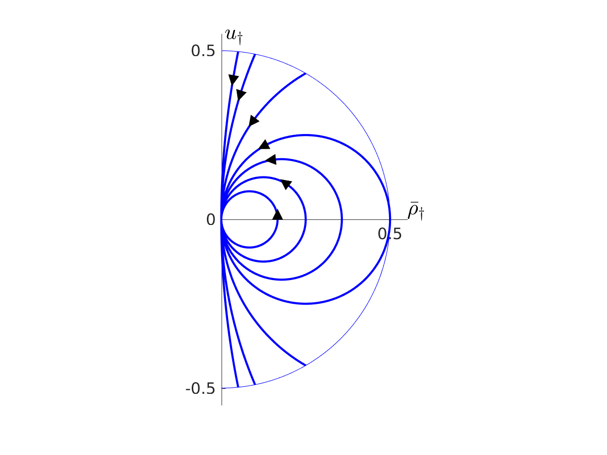
The Lagrangian variables are given by the characteristics defined as $y_{t}(t,\xi)=u(t,y(t,\xi))$ and the Lagrangian velocity $U(t,\xi)=u(t,y(t,\xi))$ . In the case of the M2CH system, we need to introduce more variables to be able to handle the blow-up of the solution. Here, we follow the approach presented in [16, 25] which is very close the one introduced in [14, 21]. Once the system of equations is completely rewritten in term of purely Lagrangian variables, semi-linearities in the system enable us to obtain global solutions. Thus, the Lagrangian system defines the solutions, which are then mapped back to Eulerian variables in order to obtain some weak solutions to the original M2CH system. We show that the existence of the pointwise invariant implies the existence of multipeakon solutions but, even if this invariant can be expressed in term of purely Lagrangian variables, its form becomes then intricate. However, this fundamental invariance property is preserved by the change of Lagrangian variables so that the existence of multipeakon can also be obtained in the Lagrangian setting, see [20] for the corresponding work in the case of the CH equation. In section 5, we derive the multipeakon equations directly from the system (1.7) and not as in [23] where a discretization of the Hamiltionian is used. We compute explicit solutions in the case of the anti-symmetric peakon-antipeakon solution. We discover an interesting dynamic in this case, which can be decomposed in three different cases. For all cases, the peaks collide but there are different behaviors when the peaks move away from each other, after collision. In the first case, there is not enough potential energy in the system to retain the particles from completely departing from each other. In the second case, the potential energy prevents them to do so. We can compare the situation to a classical discrete mechanical system where Hooke’s law is used to model the elastic forces. Such elastic forces act in both ways. They are repulsive when particles approach each other, over a given equilibrium state, and attractive when the particle move far away from each other. For M2CH, we observe that the potential energy does not yield a repulsive force that is strong enough to prevent collision but its attractive effect can prevent the fully departure of the peaks from each others. The solution in this case is periodic and we finally end up with a oscillatory system where the kinetic energy and the potential energy vanishes one after the other, as for a standard pendulum. This type of solution has not been observed for CH or 2CH. The last case in the description of the dynamics is the limiting case, where we do not obtain a periodic solution but the peaks are slowed down by the attractive force until their velocity vanishes. The position of the (left) right particle tends to (minus) infinity while their velocity tend to zero, see Figure 1.

2. Conservation laws

For the M2CH system, we define the kinetic energy as

(2.1)

E^{\text{kin}}(t)=\frac{1}{2}\int_{\mathbb{R}}(u^{2}+u_{x}^{2})(t,x)\,dx.

The proper definition of kinetic energy from physics is $\frac{1}{2}\int_{\mathbb{R}}\rho u^{2}\,dx$ . However, we are going to see that the term defined in (2.1) plays a role which resembles the one of the kinetic energy in standard physical systems and that is why we use this terminology. Using the same type of analogy, we refer to the quantity $E^{\text{pot}}$ defined below as the potential energy,

(2.2)

E^{\text{pot}}(t)=\frac{1}{2}\int_{\mathbb{R}}({\bar{\rho}}^{2}+{\bar{\rho}}_{x}^{2})(t,x)\,dx.

The total energy is then given by

(2.3)

E^{\text{tot}}(t)=\frac{1}{2}\int_{\mathbb{R}}(u^{2}+u_{x}^{2}+{\bar{\rho}}^{2}+{\bar{\rho}}_{x}^{2})(t,x)dx.

The M2CH system can be derived from a variational principle for the Lagrangian

(2.4)

\mathcal{L}=E^{\text{kin}}-E^{\text{pot}}.

We do not give the details for this computation and refer instead to [15]. The invariance of the Lagrangian with respect to time implies through Noether’s theorem that the total energy as defined in (2.3) is preserved in time. More precisely, we have the following conservation law for the energy,

(2.5)

(u^{2}+u_{x}^{2}+{\bar{\rho}}^{2}+{\bar{\rho}}_{x}^{2})_{t}+(u(u^{2}+u_{x}^{2}+{\bar{\rho}}^{2}+{\bar{\rho}}_{x}^{2}))_{x}=\\ \left(u^{3}-2Pu-2{\bar{\rho}}\mathcal{H}^{-1}(\rho u)+2u\bar{\rho}^{2}\right)_{x}.

Let us derive (2.5) from (1.7). One can prove that for any smooth function $q(t,x)$ which satisfies

(2.6)

q_{t}+uq_{x}+Q=0

for some given smooth $Q$ , one has

(2.7)

(q^{2}+q_{x}^{2})_{t}+(u(q^{2}+q_{x}^{2}))_{x}=-q_{x}^{2}u_{x}+u_{x}q^{2}-2qQ-2q_{x}Q_{x}.

We let the reader check this property. From (1.7b), we have

{\bar{\rho}}_{t}+u{\bar{\rho}}_{x}+\mathcal{H}^{-1}(\rho u)_{x}-u\mathcal{H}^{-1}\rho_{x}=0.

Let us define

Q=\mathcal{H}^{-1}(\rho u)_{x}-u\mathcal{H}^{-1}\rho_{x}.

After some computations, we get

Q_{x}=\mathcal{H}^{-1}(\rho u)-u_{x}{\bar{\rho}}_{x}-u{\bar{\rho}}.

Hence,

{\bar{\rho}}_{x}Q_{x}+{\bar{\rho}}Q=({\bar{\rho}}\mathcal{H}^{-1}(\rho u))_{x}-u_{x}{\bar{\rho}}_{x}^{2}-2u{\bar{\rho}}{\bar{\rho}}_{x}.

Then, we apply (2.7) for $q={\bar{\rho}}$ and get

(2.8)

({\bar{\rho}}^{2}+{\bar{\rho}}_{x}^{2})_{t}+(u({\bar{\rho}}^{2}+{\bar{\rho}}_{x}^{2}))_{x}=-2({\bar{\rho}}\mathcal{H}^{-1}(\rho u))_{x}+u_{x}({\bar{\rho}}_{x}^{2}-{\bar{\rho}}^{2})+2({\bar{\rho}}^{2}u)_{x}

Now, we set

Q=P_{x}

and we apply (2.7) for $q=u$ and get

(2.9)

(u^{2}+u_{x}^{2})_{t}+(u(u^{2}+u_{x}^{2}))_{x}=(u^{3}-2uP)_{x}+2u_{x}(\mathcal{H}P-u^{2}-\frac{1}{2}u_{x}^{2})

We sum up (2.8) and (2.9) and obtain

(u^{2}+u_{x}^{2}+{\bar{\rho}}^{2}+{\bar{\rho}}_{x}^{2})_{t}+(u(u^{2}+u_{x}^{2}+{\bar{\rho}}^{2}+{\bar{\rho}}_{x}^{2}))_{x}=\\ \left(u^{3}-2Pu-2{\bar{\rho}}\mathcal{H}^{-1}(\rho u)+2u\bar{\rho}^{2}\right)_{x}+2u_{x}\left(\mathcal{H}P-u^{2}-\frac{1}{2}u_{x}^{2}+\frac{1}{2}{\bar{\rho}}_{x}^{2}-\frac{1}{2}{\bar{\rho}}^{2}\right).

The last of the two terms on the right-hand side vanishes because of (1.7c) so that the conservation law (2.5) follows.

3. Lagrangian variables

In this section, we describe how the M2CH system (1.7) can be rewritten in Lagrangian variables to obtain a system which is formally equivalent but whose linear structure can be used to prove the global existence of solutions. In this section the derivation of the equivalent system is only formal. Once the system is obtained, the construction of the solution in Lagrangian variables and the mapping back to the original Eulerian variables can be done rigorously, see [16]. We introduce the characteristics defined as

(3.1)

y_{t}(t,\xi)=u(t,y(t,\xi)),

the Lagrangian velocity defined as

(3.2)

U(t,\xi)=u(t,y(t,\xi)),

the cumulative total energy distribution defined as

(3.3)

H(t,\xi)=\int_{-\infty}^{y(t,\xi)}(u^{2}+u_{x}^{2}+{\bar{\rho}}^{2}+{\bar{\rho}}_{x}^{2})(t,x)\,dx,

the Lagrangian regularized potential energy defined as

(3.4)

{\bar{r}}(t,\xi)={\bar{\rho}}(t,y(t,\xi)),

and, finally,

(3.5)

{\bar{s}}(t,\xi)={\bar{\rho}}_{x}(t,y(t,\xi)).

We will assume in the remaining of this formal derivation that the derivative $y_{\xi}$ does not vanish. After differentiating (3.4) and (3.5), we observe that, formally,

(3.6)

{\bar{r}}_{\xi}={\bar{s}}y_{\xi}

and

(3.7)

\bar{s}_{\xi}={\bar{r}}y_{\xi}-\rho(t,y)y_{\xi}.

The inverse Helmholtz operator can be written using Green’s function as

(3.8)

[\mathcal{H}^{-1}q](x)=\frac{1}{2}\int_{\mathbb{R}}e^{-\left|x-z\right|}q(z)\,dz.

Hence, we get from the definition (1.7c) of $P$ that

P(t,x)=\frac{1}{4}\int_{\mathbb{R}}e^{-\left|x-z\right|}((u^{2}+u_{x}^{2}+{\bar{\rho}}^{2}+{\bar{\rho}}_{x}^{2})+(u^{2}-2{\bar{\rho}}_{x}^{2}))(t,z)\,dz.

We change to Lagrangian variables and use the definition (3.3) of $H$ and the identity (3.5) to get

(3.9)

P(t,y)=\frac{1}{4}\int_{\mathbb{R}}e^{-\left|y(t,\xi)-y(t,\eta)\right|}(H_{\xi}(t,\eta)+(U^{2}(t,\eta)-2{\bar{s}}^{2}(t,\eta))y_{\xi}(t,\eta))\,d\eta.

The change to Lagrangian variables has the recognized advantage to get rid of the first non-linear term in (1.7a), which becomes

(3.10)

U_{t}(t,\xi)=-P_{x}(t,y(t,\xi))

Introducing

(3.11)

Q(t,\xi)=-\frac{1}{4}\int_{\mathbb{R}}\sign(\xi-\eta)e^{-\left|y(t,\xi)-y(t,\eta)\right|}\Big(H_{\xi}(t,\eta)\\ +(U^{2}(t,\eta)-2{\bar{s}}^{2}(t,\eta))y_{\xi}(t,\eta)\Big)\,d\eta,

and assuming that $y_{\xi}$ remains strictly positive, we can differentiate $P$ in (3.9) and obtain that

P_{x}(t,y(t,\xi))y_{\xi}(t,\xi)=Q(t,\xi)y_{\xi}(t,\xi).

We simplify the above expression by $y_{\xi}$ and thus (3.10) yields

(3.12)

U_{t}=-Q.

Following the same lines we introduce the integrated variables


(3.13a)	$\displaystyle R(t,\xi)$	$\displaystyle=\frac{1}{2}\int_{\mathbb{R}}e^{-\left\|y(t,\xi)-y(t,\eta)\right\|}U_{\xi}(t,\eta){\bar{r}}(t,\eta)\,d\eta,$
(3.13b)	$\displaystyle S(t,\xi)$	$\displaystyle=\frac{1}{2}\int_{\mathbb{R}}e^{-\left\|y(t,\xi)-y(t,\eta)\right\|}U_{\xi}(t,\eta){\bar{s}}(t,\eta)\,d\eta,$
(3.13c)	$\displaystyle V(t,\xi)$	$\displaystyle=-\frac{1}{2}\int_{\mathbb{R}}\sign(\xi-\eta)e^{-\left\|y(t,\xi)-y(t,\eta)\right\|}U_{\xi}(t,\eta){\bar{r}}(t,\eta)\,d\eta,$
(3.13d)	$\displaystyle W(t,\xi)$	$\displaystyle=-\frac{1}{2}\int_{\mathbb{R}}\sign(\xi-\eta)e^{-\left\|y(t,\xi)-y(t,\eta)\right\|}U_{\xi}(t,\eta){\bar{s}}(t,\eta)\,d\eta,$

and we obtain that

(3.14)

R_{\xi}=Vy_{\xi}\quad\text{ and }\quad S_{\xi}=Wy_{\xi}.

Moreover, after differentiation, we get

(3.15)

V_{\xi}=-U_{\xi}{\bar{r}}+Ry_{\xi}\quad\text{ and }\quad W_{\xi}=-U_{\xi}{\bar{s}}+Sy_{\xi}.

The conservation law (2.5) gives

(3.16)

H_{t}=\left(u^{3}-2Pu-2\bar{\rho}\mathcal{H}^{-1}(\rho u)+2u{\bar{\rho}}^{2}\right)(t,y).

Recalling that $\rho={\bar{\rho}}-{\bar{\rho}}_{xx}$ , direct computations yield that

{\bar{\rho}}\mathcal{H}^{-1}(\rho u)={\bar{\rho}}\mathcal{H}^{-1}({\bar{\rho}}u-({\bar{\rho}}u)_{xx}+(u_{x}{\bar{\rho}})_{x}+u_{x}{\bar{\rho}}_{x})=u{\bar{\rho}}^{2}+{\bar{\rho}}R_{x}+{\bar{\rho}}S

and (3.16) can be rewritten as

(3.17)

H_{t}=U^{3}-2PU-2{\bar{r}}(S+V).

Note that in (3.17), we slightly abused the notations and denoted $P(t,y)$ as $P(t,\xi)$ . We continue to do so in the remaining. Differentiating $P$ and $Q$ gives us

(3.18)		$\displaystyle P_{\xi}$	$\displaystyle=Qy_{\xi},$
(3.19)		$\displaystyle Q_{\xi}$	$\displaystyle=-\frac{1}{2}H_{\xi}-(\frac{1}{2}U^{2}-{\bar{s}}^{2}-P)y_{\xi}.$

For the Lagrangian regularized potential energy density, (1.7b) yields

(3.20)

{\bar{r}}_{t}=-(R+W).

Let us now gather the governing equations we have obtained in (3.1), (3.12), (3.17), and (3.20). We have seen that the governing equations (1.7) are formally equivalent to the system


(3.21a)	$\displaystyle y_{t}$	$\displaystyle=U,$
(3.21b)	$\displaystyle U_{t}$	$\displaystyle=-Q,$
(3.21c)	$\displaystyle H_{t}$	$\displaystyle=U^{3}-2PU-2{\bar{r}}(S+V),$
(3.21d)	$\displaystyle{\bar{r}}_{t}$	$\displaystyle=-(R+W),$
(3.21e)	$\displaystyle{\bar{s}}_{t}$	$\displaystyle=-(S+V),$

where the quantities $P$ , $Q$ , $R$ , $S$ , $V$ , and $W$ are defined in (3.9), (3.11), and (3.13), respectively. We can differentiate the first four equations in (3.21) and obtain


(3.22a)	$\displaystyle y_{\xi,t}$	$\displaystyle=U_{\xi},$
(3.22b)	$\displaystyle U_{\xi,t}$	$\displaystyle=\frac{1}{2}H_{\xi}+\Big(\frac{1}{2}U^{2}-{\bar{s}}^{2}-P\Big)y_{\xi},$
(3.22c)	$\displaystyle H_{\xi,t}$	$\displaystyle=\Big(3U^{2}-2P+2{\bar{r}}^{2}\Big)U_{\xi}-2\Big(QU+{\bar{r}}(V+W)\Big)y_{\xi}-2\Big(S+V\Big){\bar{r}}_{\xi},$
(3.22d)	$\displaystyle{\bar{r}}_{\xi,t}$	$\displaystyle={\bar{s}}U_{\xi}-(S+V)y_{\xi}.$

The system (3.22) reveals the semi-linear nature of the equivalent system. Indeed, the system is semi-linear with respect to the derivatives $y_{\xi}$ , $U_{\xi}$ , $H_{\xi}$ and ${\bar{r}}_{\xi}$ in the sense that all the other terms (included ${\bar{s}}$ ) that enter the system are of higher regularity than these derivatives. The semi-linearity of the system is essential in the proof of the existence of solutions using Picard’s argument. The variable $H$ is now considered as an independent variable but when we introduced it in (3.3), it was clearly dependent on the other variables. Changing variables in (3.3) gives us

(3.23)

y_{\xi}H_{\xi}=(U^{2}+{\bar{r}}^{2}+\bar{s}^{2})y_{\xi}^{2}+U_{\xi}^{2},

and it can be shown that the governing system (3.21) preserves this identity, if it holds initially. Thus, we have decoupled $H$ from the other variables, in particular to obtain a semi-linear system, but (3.23) shows that the variables are not truly independent as they are constrained by the system to remain on the “manifold” defined by (3.23). As shown in [16], the system of ordinary differential equations (3.21) has global solutions in a suitable Banach space. In particular,

(3.24)

y-\id,H\in L^{\infty}(\mathbb{R})\quad y_{\xi}-1,U,U_{\xi},{\bar{r}},{\bar{r}}_{\xi},{\bar{s}},H_{\xi}\in L^{2}(\mathbb{R})\cap L^{\infty}(\mathbb{R}).

These global solutions in Lagrangian coordinates can then be mapped to global weak conservative solutions of the M2CH system as in [21] in the case of the CH equation. To be more specific, one has for each fixed time $t$ , cf. [16, Definition 4.4], that

(3.25)

u(x)=U(\xi),\quad{\bar{\rho}}(x)={\bar{r}}(\xi),\quad\text{ and }\quad{\bar{\rho}}_{x}(x)={\bar{s}}(\xi)

for any $\xi$ , such that $x=y(\xi)$ and

\mu(B)=\int_{\{x\in y^{-1}(B)\}}H_{\xi}(\xi)d\xi\quad\text{ for any Borel set }B,

where $\mu$ denotes the energy distribution measure. Since $\bar{s}(t,\cdot)\in L^{\infty}(\mathbb{R})$ , it follows from (3.25) that ${\bar{\rho}}_{x}$ remains also bounded in $L^{\infty}(\mathbb{R})$ . In particular, it means that the blow-up of the solution only occurs when $u_{x}$ becomes unbounded, as in the CH case, the additional variable ${\bar{\rho}}$ of M2CH does not blow up. Before closing this section, we introduce the Lagrangian potential energy $r$ as

(3.26)

r(t,\xi)=\rho(t,y(t,\xi))y_{\xi}(t,\xi).

As opposed to all the other Lagrangian variables introduced until now $(y-\xi,U,H,{\bar{r}},{\bar{s}})$ , the Lagrangian variable $r$ is not generally bounded in $L^{\infty}(\mathbb{R})$ . Formally, ${\bar{r}}$ can be obtained from $r$ as

(3.27)

{\bar{r}}(t,\xi)=\frac{1}{2}\int_{\mathbb{R}}e^{-\left|y(t,\xi)-y(t,\eta)\right|}r(t,\eta)d\eta

and we also have the following relation between ${\bar{r}}$ , ${\bar{s}}$ and $r$ ,

(3.28)

r=-{\bar{s}}_{\xi}+{\bar{r}}y_{\xi},

from (3.7). From the definition of $r$ , (3.26), and the transport equation (1.1b), we expect

(3.29)

r_{t}=0

This result can also be derived directly from the equivalent system (3.21) in purely Lagrangian variables. Indeed, after differentiating (3.28) with respect to time, we get

r_{t}=-{\bar{s}}_{\xi t}+{\bar{r}}_{t}y_{\xi}+{\bar{r}}y_{\xi t}.

We use (3.21) and obtain

r_{t}=+(V_{\xi}+S_{\xi})-(R+W)y_{\xi}+{\bar{r}}U_{\xi}.

From (3.15) and (3.14), we obtain as expected that $r_{t}=0$ .

4. Relabeling symmetry and local invariants

4.1. The case of the scalar Camassa–Holm equation

As we mentioned in the introduction, the CH equation can be derived from a variational principle, see [9] for a more thorough presentation. In the case of the CH equation, there is no potential energy and the Lagrangian is given by the kinetic energy only,

\mathcal{L}_{\text{CH}}=\frac{1}{2}\int_{\mathbb{R}}(u^{2}+u_{x}^{2})(t,x)\,dx.

The variation has to be done with respect to the particle path. We follow the notations from [9] and denote the particle path by $\varphi(t,\xi)$ , instead of $y(t,\xi)$ as in the previous section. After a change of variable, we can rewrite $\mathcal{L}_{\text{CH}}$ as

(4.1)

\mathcal{L}_{\text{CH}}(\varphi)=\frac{1}{2}\int_{\mathbb{R}}\left(\varphi_{t}^{2}\varphi_{\xi}+\frac{\varphi_{t\xi}^{2}}{\varphi_{\xi}}\right)(t,\xi)\,d\xi.

The group of diffeomorphism on $\mathbb{R}$ lets the Lagrangian invariant with respect to the group action of relabeling. For a given diffeomorphism $f$ , the relabeling transformation of $\varphi(t,\xi)$ , with respect to $f$ , is given by $\varphi\hskip-1.42262pt\circ\hskip-1.42262ptf=\varphi(t,f(\xi))$ . We can check directly that

\mathcal{L}_{\text{CH}}(\varphi\hskip-1.42262pt\circ\hskip-1.42262ptf)=\frac{1}{2}\int_{\mathbb{R}}\left((\varphi_{t}\hskip-1.42262pt\circ\hskip-1.42262ptf)^{2}(\varphi_{\xi}\hskip-1.42262pt\circ\hskip-1.42262ptf)f_{\xi}+\frac{(\varphi_{t\xi}\hskip-1.42262pt\circ\hskip-1.42262ptf)^{2}f_{\xi}^{2}}{(\varphi_{\xi}\hskip-1.42262pt\circ\hskip-1.42262ptf)f_{\xi}}\right)(t,\xi)\,d\xi=\mathcal{L}_{\text{CH}}(\varphi),

after a change of variable. Noether’s theorem tells us that to every one-dimensional symmetry group which let the Lagrangian invariant, there corresponds a conservation law. For the group of diffeomorphism, the tangent space is formally isomorphic to $C^{\infty}(\mathbb{R})$ , which is of infinite dimension, so that we expect infinitely many invariants. Let us first shortly present the Noether’s argument in a finite dimensional setting, that is how a symmetry leads to an invariant. We consider $q\in\mathbb{R}^{n}$ and the Lagrangian $\mathcal{L}(q,\dot{q})$ . We assume that $\mathcal{L}$ admits a one-dimensional symmetry group. Keeping this presentation informal, we simply assume that there exists a smooth mapping $S:\mathbb{R}\times\mathbb{R}^{n}\to\mathbb{R}^{n}$ , which represents the one-dimensional group action, such that $S(0,\cdot)=\id$ , and we denote $q_{\varepsilon}(t)=S(\varepsilon,q(t))$ . The invariance of the Lagrangian takes the form

(4.2)

\mathcal{L}(q_{\varepsilon}(t),\dot{q}_{\varepsilon}(t))=\mathcal{L}(q(t),\dot{q}(t)).

The Euler-Lagrange equations for the solution are

(4.3)

\frac{d}{dt}\left(\frac{\partial\mathcal{L}}{\partial\dot{q}}\right)=\frac{\partial\mathcal{L}}{\partial q}.

We differentiate (4.2) with respect to $\varepsilon$ and obtain

\frac{\partial\mathcal{L}}{\partial q}\frac{\partial q_{\varepsilon}}{\partial\varepsilon}+\frac{\partial\mathcal{L}}{\partial\dot{q}}\frac{\partial\dot{q}_{\varepsilon}}{\partial\varepsilon}=0.

We set $\varepsilon=0$ and use the Euler-Lagrange equation and the previous equation to get

\frac{d}{dt}\left(\frac{\partial\mathcal{L}}{\partial\dot{q}}\right)\frac{\partial q_{\varepsilon}}{\partial\varepsilon}_{|\varepsilon=0}+\frac{\partial\mathcal{L}}{\partial\dot{q}}\frac{\partial\dot{q}_{\varepsilon}}{\partial\varepsilon}_{|\varepsilon=0}=0.

Assuming the solution is smooth, we have

\frac{\partial\dot{q}}{\partial\varepsilon}_{|\varepsilon=0}=\frac{d}{dt}\left(\frac{\partial q}{\partial\varepsilon}_{|\varepsilon=0}\right)

and therefore it follows that

(4.4)

\frac{d}{dt}\left(\frac{\partial\mathcal{L}}{\partial\dot{q}}\frac{\partial q_{\varepsilon}}{\partial\varepsilon}_{|\varepsilon=0}\right)=0,

and the quantity

\frac{\partial\mathcal{L}}{\partial\dot{q}}\frac{\partial q_{\varepsilon}}{\partial\varepsilon}_{|\varepsilon=0}

is preserved.

Let us consider now the Lagrangian $\mathcal{L}_{\text{CH}}$ . To simplify the notations we will denote the operator $\frac{\partial}{\partial\varepsilon}_{|\varepsilon=0}$ as $\delta_{\varepsilon}$ . The Lagrangian is invariant with respect to relabeling. Formally, the tangent space at the identity of the group of smooth diffeomorphisms is the space of smooth functions $C^{\infty}(\mathbb{R})$ . For any function $g\in C^{\infty}(\mathbb{R})$ in the tangent space, we define the diffeomorphism $f_{\varepsilon}(\xi)=\xi+\varepsilon g(\xi)$ and consider the one-dimensional action defined as

\varphi_{\varepsilon}=\varphi\hskip-1.42262pt\circ\hskip-1.42262ptf_{\varepsilon}.

Slightly abusing the notation, we redefine $\mathcal{L}_{\text{CH}}$ as

\mathcal{L}_{\text{CH}}(\varphi,\psi)=\frac{1}{2}\int_{\mathbb{R}}\left(\psi^{2}\varphi_{\xi}+\frac{\psi_{\xi}^{2}}{\varphi_{\xi}}\right)(t,\xi)\,d\xi,

so that $\mathcal{L}_{\text{CH}}(\varphi,\partial_{t}\varphi)$ is equal to $\mathcal{L}_{\text{CH}}(\varphi)$ , as introduced in (4.1). The invariance of $\mathcal{L}_{\text{CH}}$ with respect to relabeling implies

\mathcal{L}_{\text{CH}}(\varphi_{\varepsilon},\partial_{t}\varphi_{\varepsilon})=\mathcal{L}_{\text{CH}}(\varphi,\partial_{t}\varphi),

for all $\varepsilon\in\mathbb{R}$ , small enough. Following the same steps as before in the finite dimensional case, we end up with the following conservation law, corresponding to (4.4),

(4.5)

\frac{\partial}{\partial t}\left<\frac{\delta\mathcal{L}_{\text{CH}}}{\delta\psi},\delta_{\varepsilon}\varphi\right>=0.

Let us give a precise meaning to each of the expressions entering (4.5). We have

\left<\frac{\delta\mathcal{L}_{\text{CH}}}{\delta\psi},\delta\psi\right>=\int_{\mathbb{R}}(\psi\delta\psi\varphi_{\xi}+\frac{\psi_{\xi}}{\varphi_{\xi}}\delta\psi_{\xi})\,d\xi

so that

\frac{\delta\mathcal{L}_{\text{CH}}}{\delta\psi}=\psi\varphi_{\xi}-\left(\frac{\psi_{\xi}}{\varphi_{\xi}}\right)_{\xi}.

Let us compute $\delta_{\varepsilon}\varphi_{\varepsilon}$ . We have

\delta_{\varepsilon}\varphi_{\varepsilon}=\frac{\partial}{\partial\varepsilon}_{|\varepsilon=0}\varphi(\xi+\varepsilon g(\xi))=\varphi_{\xi}(\xi)g(\xi).

Hence, (4.5) can be rewritten as

\frac{\partial}{\partial t}\left(\int_{\mathbb{R}}\left(\varphi_{t}\varphi_{\xi}-\left(\frac{\varphi_{t\xi}}{\varphi_{\xi}}\right)_{\xi}\right)\varphi_{\xi}g\,d\xi\right)=0.

Assuming that the solution is smooth and decays sufficiently fast, it follows that

(4.6)

\int_{\mathbb{R}}\frac{\partial}{\partial t}\left(\left(\varphi_{t}\varphi_{\xi}-\left(\frac{\varphi_{t\xi}}{\varphi_{\xi}}\right)_{\xi}\right)\varphi_{\xi}\right)g\,d\xi=0,

as $g$ is independent of time. Now, we use the fact that (4.6) must hold for any $g\in C^{\infty}$ and therefore we obtain the following pointwise invariant,

\frac{\partial}{\partial t}\left(\left(\left(\varphi_{t}\varphi_{\xi}-\left(\frac{\varphi_{t\xi}}{\varphi_{\xi}}\right)_{\xi}\right)\varphi_{\xi}\right)(t,\xi)\right)=0,

for all $\xi\in\mathbb{R}$ . Using the fact that $u\hskip-1.42262pt\circ\hskip-1.42262pt\varphi=\varphi_{t}$ , $u_{x}\hskip-1.42262pt\circ\hskip-1.42262pt\varphi=\frac{\varphi_{t\xi}}{\varphi_{\xi}}$ and $u_{xx}\hskip-1.42262pt\circ\hskip-1.42262pt\varphi=\frac{(u_{x}\hskip-1.42262pt\circ\hskip-1.42262pt\varphi)_{\xi}}{\varphi_{\xi}}$ , we can rewrite the pointwise invariant above in the form of

(4.7)

\frac{\partial}{\partial t}((u-u_{xx})(t,\varphi(t,\xi))\varphi_{\xi}^{2}(t,\xi))=0.

Note that, in fact, the pointwise invariant equation (4.7) can be used to derive the CH equation in a rather straightforward way. To see that, let us denote $m=\mathcal{H}u$ and expand (4.7). We obtain

(m_{t}\hskip-1.42262pt\circ\hskip-1.42262pt\varphi+m_{x}\hskip-1.42262pt\circ\hskip-1.42262pt\varphi\varphi_{t})\varphi_{\xi}^{2}+2m\hskip-1.42262pt\circ\hskip-1.42262pt\varphi\varphi_{\xi}\varphi_{t\xi}=0,

which, after using $\varphi_{t}=u\hskip-1.42262pt\circ\hskip-1.42262pt\varphi$ and $\varphi_{t\xi}=u_{x}\hskip-1.42262pt\circ\hskip-1.42262pt\varphi\varphi_{\xi}$ , yields

(m_{t}+um_{x}+2mu_{x})\hskip-1.42262pt\circ\hskip-1.42262pt\varphi\varphi_{\xi}^{2}=0,

which, whenever $\varphi_{\xi}$ does not vanish, is equivalent to the CH equation.

Multipeakon solutions, which are a special class of solutions for the CH equation, are of the form

(4.8)

u(t,x)=\sum_{i=1}^{n}p_{i}(t)e^{-|x-q_{i}(t)|}

for time-dependent coefficients $q_{i}(t)$ , which denote the position of the peaks, $p_{i}(t)$ . Such solutions were identified in the seminal paper of Camassa and Holm [3]. Here, we want to show how the existence of this special class of solutions can be inferred directly from the pointwise invariant (4.7). As the pointwise invariant is a consequence of the symmetry of the problem, we can therefore establish a rather direct connection between the symmetry of the Lagrangian and the existence of special solutions. This approach is described in detail in [20] and we sketch it here as a preparation for the case of M2CH. After applying the Helmholtz operator $\mathcal{H}$ to $u$ in (4.8), we get

(4.9)

(u-u_{xx})(t,x)=\sum_{i=1}^{N}2p_{i}(t)\delta(x-q_{i}(t)),

where $\delta(x)$ denotes the Dirac delta distribution. For some initial data that satisfies (4.8) and any point $x\in\mathbb{R}$ away from the singularities, meaning that it does not coincide with any of the $q_{i}$ , we have $(u-u_{xx})(x)=0$ . After denoting $x(t)=y(t,\xi)$ the characteristic starting at $x$ , the pointwise invariant (4.7) yields $(u-u_{xx})(t,x(t))=0$ , as long as $y_{\xi}(t,\xi)\neq 0$ . Hence, the structure given by (4.9), which defines the multipeakons, is preserved. The formulation given by (4.9) cannot handle the collision of peaks as some of the coefficients $p_{i}$ tend to $\pm\infty$ in this case. To handle such case, we have to switch to the Lagrangian formulation. The pointwise conservation equation plays then an essential role when showing that the multipeakon structure is preserved. Between two neighboring peaks, say $q_{i}(t)$ and $q_{i+1}(t)$ , we have to show that $(u-u_{xx})(t,x)=0$ for all $x\in(q_{i}(t),q_{i+1}(t))$ . The peaks follow the characteristics so that, in Lagrangian coordinates, the region between the two peaks given as $\{(t,x)\ |\ q_{i}(t)<x<q_{i+1}(t)\}$ , which is curved in Eulerian coordinates, becomes rectangular, that is $\{(t,\xi)\ |\ \xi_{i}<\xi<\xi_{i+1}\}$ . Once the pointwise conservation equation is established for each of such regions, we can then deduce that the solution is indeed a multipeakon solution. The rigorous presentation of this approach is given in [20].

4.2. The case of the modified system

The Lagrangian for the M2CH system is given in (2.4). Let us rewrite the potential energy in terms of the Lagrangian variables we have introduced. We have

E^{\text{pot}}=\frac{1}{2}\int_{\mathbb{R}}({\bar{\rho}}-{\bar{\rho}}_{xx}){\bar{\rho}}\,dx=\frac{1}{2}\int_{\mathbb{R}}\rho(x){\bar{\rho}}(x)\,dx.

We change to Lagrangian variable and obtain

E^{\text{pot}}=\frac{1}{2}\int_{\mathbb{R}}{\bar{r}}(\xi)r(\xi)\,d\xi.

We use the expression for ${\bar{r}}$ derived in (3.27) and get

E^{\text{pot}}=\frac{1}{4}\int_{\mathbb{R}^{2}}e^{-\left|\varphi(t,\xi)-\varphi(t,\eta)\right|}r(t,\eta)r(t,\xi)\,d\eta d\xi.

The relabeling transformation for a density variable such as $r$ is defined as $r\mapsto r\hskip-1.42262pt\circ\hskip-1.42262ptff_{\xi}$ for any $f\in\text{diff}(\mathbb{R})$ . For such transformations, we can check that the potential energy $E^{\text{pot}}$ is invariant. In [15], when we proceed with the variation for the 2CH system, the density $\rho$ is treated as a function of $\varphi$ so that the variation with respect to $\rho$ is not computed independently. Here, we use a different approach by decoupling the variables and introducing a Lagrangian multiplier function $\lambda$ to enforce the mass conservation, that is $r_{t}=0$ . Let $X=(\varphi,r,\lambda)$ , we consider the Lagrangian defined as

(4.10)

\mathcal{L}(X,\partial_{t}X)=\frac{1}{2}\int_{\mathbb{R}}\left(\varphi_{t}^{2}\varphi_{\xi}+\frac{\varphi_{t\xi}^{2}}{\varphi_{\xi}}\right)(t,\xi)\,d\xi\\ -\frac{1}{4}\int_{\mathbb{R}^{2}}e^{-\left|\varphi(t,\xi)-\varphi(t,\eta)\right|}r(t,\eta)r(t,\xi)\,d\eta d\xi\\ -\int_{\mathbb{R}}\lambda(t,\xi)r_{t}(t,\xi)\,d\xi.

We derive the Euler-Lagrange equation for this Lagrangian. Computations which we only sketch here give us

(4.11a)	$\frac{\delta\mathcal{L}}{\delta\varphi}=-\frac{1}{2}(\varphi_{t}^{2})_{\xi}+\frac{1}{2}\left(\frac{\varphi_{t,\xi}^{2}}{\varphi_{\xi}^{2}}\right)_{\xi}\\ +\frac{r}{2}\int_{\mathbb{R}}\sign(\varphi(t,\xi)-\varphi(t,\eta))e^{-\left\|\varphi(t,\xi)-\varphi(t,\eta)\right\|}r(t,\eta)\,d\eta$
with
(4.11b)	$\frac{\delta\mathcal{L}}{\delta[\varphi_{t}]}=\varphi_{t}\varphi_{\xi}-\left(\frac{\varphi_{t,\xi}}{\varphi_{\xi}}\right)_{\xi}$
and

(4.11c)	$\displaystyle\frac{\delta\mathcal{L}}{\delta r}$	$\displaystyle=-\frac{1}{2}\int_{\mathbb{R}}e^{-\left\|\varphi(t,\xi)-\varphi(t,\eta)\right\|}r(t,\eta)\,d\eta,$	$\displaystyle\frac{\delta\mathcal{L}}{\delta[r_{t}]}$	$\displaystyle=-\lambda,$
(4.11d)	$\displaystyle\frac{\delta\mathcal{L}}{\delta\lambda}$	$\displaystyle=-r_{t},$	$\displaystyle\frac{\delta\mathcal{L}}{\delta[\lambda_{t}]}$	$\displaystyle=0.$

We consider a diffeomorphism $\varphi$ and a perturbation $\delta\varphi$ , then $r(t,\xi)$ is perturbed by a corresponding $\delta r(t,\xi)$ . Thus varying the integral defined

(4.12)

\mathcal{L}^{\text{pot}}=\frac{1}{4}\int_{\mathbb{R}^{2}}e^{-|\varphi(t,\xi)-\varphi(t,\eta)|}r(t,\eta)r(t,\xi)d\eta d\xi,

with respect to $r$ yields

	$\displaystyle\left<\frac{\delta\mathcal{L}^{\text{pot}}}{\delta r},\delta r\right>$	$\displaystyle=\frac{1}{4}\int_{\mathbb{R}^{2}}e^{-\|\varphi(t,\xi)-\varphi(t,\eta)\|}(\delta r(t,\eta)r(t,\xi)+r(t,\eta)\delta r(t,\xi))d\eta d\xi$
		$\displaystyle=\frac{1}{2}\int_{\mathbb{R}}\left(\int_{\mathbb{R}}e^{-\|\varphi(t,\xi)-\varphi(t,\eta)\|}r(t,\eta)d\eta\right)\delta r(t,\xi)d\xi,$

since we can interchange the order of integration. Varying $\mathcal{L}^{\text{pot}}$ with respect to $\varphi$ yields

		$\displaystyle\Big<\frac{\delta\mathcal{L}^{\text{pot}}}{\delta\varphi},\delta\varphi\Big>$
		$\displaystyle=-\frac{1}{4}\int_{\mathbb{R}^{2}}\sign(\varphi(t,\xi)-\varphi(t,\eta))e^{-\|\varphi(t,\xi)-\varphi(t,\eta)\|}r(t,\eta)r(t,\xi)(\delta\varphi(t,\xi)-\delta\varphi(t,\eta))d\eta d\xi$
		$\displaystyle=-\frac{1}{4}\int_{\mathbb{R}}\int_{\mathbb{R}}\sign(\varphi(t,\xi)-\varphi(t,\eta))e^{-\|\varphi(t,\xi)-\varphi(t,\eta)\|}r(t,\eta)d\eta r(t,\xi)\delta\varphi(t,\xi)d\xi$
		$\displaystyle\qquad+\frac{1}{4}\int_{\mathbb{R}}\int_{\mathbb{R}}\sign(\varphi(t,\xi)-\varphi(t,\eta))e^{-\|\varphi(t,\xi)-\varphi(t,\eta)\|}r(t,\eta)\delta\varphi(t,\eta)d\eta r(t,\xi)d\xi$
		$\displaystyle=-\frac{1}{2}\int_{\mathbb{R}}\left(\int_{\mathbb{R}}\sign(\varphi(t,\xi)-\varphi(t,\eta))e^{-\|\varphi(t,\xi)-\varphi(t,\eta)\|}r(t,\eta)d\eta r(t,\xi)\right)\delta\varphi(t,\xi)d\xi,$

since we can again interchange the order of integration. The Euler-Lagrange equation

\frac{d}{dt}\left(\frac{\delta\mathcal{L}}{\delta[X_{t}]}\right)=\frac{\delta\mathcal{L}}{\delta X}

yields

(4.13)

r_{t}=0,

from (4.11d) and

(4.14)

\lambda_{t}=\frac{1}{2}\int_{\mathbb{R}}e^{-\left|\varphi(t,\xi)-\varphi(t,\eta)\right|}r(t,\eta)\,d\eta,

from (4.11c). Using the variable ${\bar{r}}$ defined as in (3.27), we rewrite (4.14) as

(4.15)

\lambda_{t}={\bar{r}}.

We can also rewrite (4.11a) as

(4.16)

\frac{\delta\mathcal{L}}{\delta\varphi}=-\frac{1}{2}(\varphi_{t}^{2})_{\xi}+\frac{1}{2}\left(\frac{\varphi_{t,\xi}^{2}}{\varphi_{\xi}^{2}}\right)_{\xi}-r\frac{{\bar{r}}_{\xi}}{\varphi_{\xi}}.

Then, (4.16) and (4.11b) yields

(4.17)

\frac{d}{dt}\left(\varphi_{t}\varphi_{\xi}-\left(\frac{\varphi_{t,\xi}}{\varphi_{\xi}}\right)_{\xi}\right)=-\frac{1}{2}(\varphi_{t}^{2})_{\xi}+\frac{1}{2}\left(\frac{\varphi_{t,\xi}^{2}}{\varphi_{\xi}^{2}}\right)_{\xi}-r\frac{{\bar{r}}_{\xi}}{\varphi_{\xi}}.

The variable $r$ has been introduced as a primary variable, but since $r_{t}=0$ , its dynamic is trivial. Setting $\rho\hskip-1.42262pt\circ\hskip-1.42262pt\varphi=\frac{r}{\varphi_{\xi}}$ , $r_{t}=0$ implies that

(\rho_{t}+(u\rho)_{x})\hskip-1.42262pt\circ\hskip-1.42262pt\varphi\varphi_{\xi}=0,

so that $\rho$ is indeed the density, if it is initially set as such. Moreover we have

{\bar{r}}=\frac{1}{2}\int_{\mathbb{R}}e^{-\left|\varphi(t,\xi)-\varphi(t,\eta)\right|}r(t,\eta)\,d\eta={\bar{\rho}}\hskip-1.42262pt\circ\hskip-1.42262pt\varphi.

Hence,

r\frac{{\bar{r}}_{\xi}}{\varphi_{\xi}}=\rho\hskip-1.42262pt\circ\hskip-1.42262pt\varphi{\bar{\rho}}_{x}\hskip-1.42262pt\circ\hskip-1.42262pt\varphi\varphi_{\xi}.

After some computation, we can then see that (4.17) is equivalent to

(m_{t}+um_{x}+2mu_{x}+\rho{\bar{\rho}}_{x})\hskip-1.42262pt\circ\hskip-1.42262pt\varphi\varphi_{\xi}=0,

that is (1.1a), when $\varphi_{\xi}$ does not vanish. Let us now consider the action of relabeling on $\mathcal{L}$ and derive pointwise invariants. The action of the group on the Lagrangian multiplier $\lambda$ is given by $(\lambda,f)\mapsto\lambda\hskip-1.42262pt\circ\hskip-1.42262ptf$ , for any diffeomorphism $f$ . As in the scalar case of the CH equation, we consider for any $g\in C^{\infty}(\mathbb{R})$ the one-dimensional subgroup $f_{\varepsilon}(\xi)=\xi+\varepsilon g(\xi)$ of diffeomorphisms. Using the notations introduced previously, we get

(4.18)

\delta_{\varepsilon}\varphi=\varphi_{\xi}g,\quad\delta_{\varepsilon}r=r_{\xi}g+rg_{\xi}=(rg)_{\xi},\quad\delta_{\varepsilon}\lambda=\lambda_{\xi}g.

The pointwise conservation law (4.5) becomes

(4.19)

\frac{\partial}{\partial t}\left(\frac{\delta\mathcal{L}_{\text{CH}}}{\delta[\varphi_{t}]}\delta_{\varepsilon}\varphi+\frac{\delta\mathcal{L}_{\text{CH}}}{\delta[r_{t}]}\delta_{\varepsilon}r+\frac{\delta\mathcal{L}_{\text{CH}}}{\delta[\lambda_{t}]}\delta_{\varepsilon}\lambda\right)=0

in this case. Hence, using (4.11b), (4.11c), (4.11d) and (4.18), we get

(4.20)

\frac{\partial}{\partial t}\left(\int_{\mathbb{R}}\left(\varphi_{t}\varphi_{\xi}-\left(\frac{\varphi_{t,\xi}}{\varphi_{\xi}}\right)_{\xi}\right)\varphi_{\xi}g\,d\xi-\int_{\mathbb{R}}\lambda(rg)_{\xi}\,d\xi\right)=0.

Assuming that the solution is smooth and decays sufficiently fast, we move the time derivative under the integral. The first integral is the same as in the scalar case. For the second one, we get, after integration by parts,

\frac{\partial}{\partial t}\left(\int_{\mathbb{R}}\lambda(rg)_{\xi}\,d\xi\right)=-\int_{\mathbb{R}}(\lambda_{\xi}r)_{t}g\,d\xi

using the fact that $r_{t}=0$ . Hence, (4.20) yields

\int_{\mathbb{R}}(m\hskip-1.42262pt\circ\hskip-1.42262pt\varphi\varphi_{\xi}^{2}+\lambda_{\xi}r)_{t}g=0,

which must hold for any function $g$ so that the pointwise conservation law for the M2CH system is given by

(4.21)

((m\hskip-1.42262pt\circ\hskip-1.42262pt\varphi+\frac{\lambda_{\xi}}{\varphi_{\xi}}\rho\hskip-1.42262pt\circ\hskip-1.42262pt\varphi)\varphi_{\xi}^{2})_{t}=0,

and the pointwise conserved quantity is

(4.22)

(m\hskip-1.42262pt\circ\hskip-1.42262pt\varphi+\frac{\lambda_{\xi}}{\varphi_{\xi}}\rho\hskip-1.42262pt\circ\hskip-1.42262pt\varphi)\varphi_{\xi}^{2}.

Again, as for the case of CH, we observe that M2CH can be derived from (4.22) in a rather straightforward manner. Using that $r_{t}=0$ and the expression (4.15) for $\lambda_{t}$ , we get

(\lambda_{\xi}r)_{t}={\bar{r}}_{\xi}r=(\rho{\bar{\rho}}_{x})\hskip-1.42262pt\circ\hskip-1.42262pt\varphi\,\varphi_{\xi}^{2},

so that (4.21) can be rewritten as

(4.23)

(m\hskip-1.42262pt\circ\hskip-1.42262pt\varphi\,\varphi_{\xi}^{2})_{t}=-(\rho{\bar{\rho}}_{x})\hskip-1.42262pt\circ\hskip-1.42262pt\varphi\,\varphi_{\xi}^{2},

and, as before for the scalar case, we can check that (4.23) implies (1.1a).

From the pointwise conservation law (4.21), we can deduce the existence of multipeakon solutions. These are solutions $(u(t,x),{\bar{\rho}}(t,x))$ of the form

(4.24)

u(t,x)=\sum_{i=1}^{n}p_{i}(t)e^{-|x-q_{i}(t)|}\quad\text{ and }\quad{\bar{\rho}}(t,x)=\sum_{i=1}^{n}s_{i}(t)e^{-|x-q_{i}(t)|}

for time-dependent coefficients $q_{i}(t)$ , which denote the position of the peaks, $p_{i}(t)$ and $s_{i}(t)$ . After applying the Helmholtz operator $\mathcal{H}$ to $u$ and ${\bar{\rho}}$ in (4.24) , we get

(4.25)

(u-u_{xx})(t,x)=\sum_{i=1}^{N}2p_{i}(t)\delta(x-q_{i}(t)),\quad\rho(t,x)=\sum_{i=1}^{N}2s_{i}(t)\delta(x-q_{i}(t)),

where $\delta(x)$ denotes the Dirac delta distribution. Let us consider some initial data that satisfies (4.25) initially. For any point $x\in\mathbb{R}$ away from the singularities, that is different from any of the $q_{i}$ , we have $(u-u_{xx})(x)=0$ and $\rho(x)=0$ . Let us denote $x(t)=y(t,\xi)$ the characteristic starting at $x$ . Since $r_{t}=0$ , we get that $\rho(t,x(t))y_{\xi}(t,\xi)=0$ , that is $\rho(t,x(t))=0$ , as long as $y_{\xi}(t,\xi)\neq 0$ . From the pointwise invariant (4.21), we infer that $(u-u_{xx})(t,x(t))=0$ , as long as $y_{\xi}(t,\xi)\neq 0$ . Hence, the structure given by (4.25), which defines the multipeakons, is preserved. The formulation given by (4.25) cannot handle the collision of peaks as some of the coefficients $p_{i}$ tend to $\pm\infty$ in this case. To do so, we have to switch to the Lagrangian formulation. To show that the multipeakon structure is preserved in the Lagrangian formulation, the pointwise conservation equation plays again an essential role but, clearly as the following computations show, the derivation is significantly less tractable. Between two neighboring peaks, say $q_{i}(t)$ and $q_{i+1}(t)$ , we have to show that $(u-u_{xx})(t,x)=0$ and $\rho(t,x)=0$ for all $x\in(q_{i}(t),q_{i+1}(t))$ . The peaks follow the characteristics so that, in Lagrangian coordinates, the region between the two peaks given as $\{(t,x)\ |\ q_{i}(t)<x<q_{i+1}(t)\}$ , which is curved in Eulerian coordinates, becomes rectangular $\{(t,\xi)\ |\ \xi_{i}<\xi<\xi_{i+1}\}$ . Once the pointwise conservation equation is established for each of such regions, we can then deduce that the solution is indeed a multipeakon solution. The rigorous presentation of this approach is given in [20] and we only sketch here how we prove the local conservation equation in the Lagrangian setting. For each rectangular region of the form defined above, we can prove that higher regularity for the Lagrangian variables is preserved by the governing equations, see [20]. Then, we can define the following quantities

(u-u_{xx})(t,y)y_{\xi}^{2}=Uy_{\xi}^{2}-U_{\xi\xi}+\frac{y_{\xi\xi}}{y_{\xi}}U_{\xi}

and

(4.26)

r=-{\bar{s}}_{\xi}+{\bar{r}}y_{\xi}.

Note that both quantities require higher regularity of the variables (existence of $U_{\xi\xi}$ , $y_{\xi\xi}$ , ${\bar{s}}_{\xi}$ ). For symplicity, we assume that $y_{\xi}$ is different from zero. This assumption can then be removed as in [20]. The pointwise conservation equation will be established in the Lagrangian setting if we can show that the quantity $M$ defined below remains equal to zero,

(4.27)

\underbrace{\frac{d}{dt}(Uy_{\xi}^{2}-U_{\xi\xi}+\frac{y_{\xi\xi}}{y_{\xi}}U_{\xi})+\bar{r}_{\xi}r+\lambda r_{t}}_{M}=0.

We have seen at the end of Section 3 that $r_{t}=0$ can be derived directly from the governing equations (3.21) in Lagrangian variables. Combining (3.19) and (3.23), we get

(4.28)

Q_{\xi}=-U^{2}y_{\xi}-\frac{1}{2}\frac{U_{\xi}^{2}}{y_{\xi}}+Py_{\xi}-\frac{1}{2}{\bar{r}}^{2}y_{\xi}+\frac{1}{2}{\bar{s}}^{2}y_{\xi}.

Now, using the governing equations (3.21), we get

M=\underbrace{(Uy_{\xi}^{2})_{t}}_{A}+\underbrace{Q_{\xi\xi}}_{B}+\frac{U_{\xi\xi}U_{\xi}}{y_{\xi}}-\underbrace{\frac{y_{\xi\xi}}{y_{\xi}}Q_{\xi}}_{C}-\frac{y_{\xi\xi}U_{\xi}^{2}}{y_{\xi}^{2}}+{\bar{r}}_{\xi}r

with

	$\displaystyle A$	$\displaystyle=-Qy_{\xi}^{2}+2UU_{\xi}y_{\xi},$
	$\displaystyle B$	$\displaystyle=-2UU_{\xi}y_{\xi}-U^{2}y_{\xi\xi}-\frac{U_{\xi\xi}U_{\xi}}{y_{\xi}}+\frac{1}{2}\frac{U_{\xi}^{2}y_{\xi\xi}}{y_{\xi}^{2}}+Qy_{\xi}^{2}+Py_{\xi\xi}$
		$\displaystyle\quad-{\bar{r}}{\bar{r}}_{\xi}y_{\xi}-\frac{{\bar{r}}^{2}}{2}y_{\xi\xi}+{\bar{s}}{\bar{s}}_{\xi}y_{\xi}+\frac{{\bar{s}}^{2}}{2}y_{\xi\xi},$
	$\displaystyle C$	$\displaystyle=-U^{2}y_{\xi\xi}-\frac{1}{2}\frac{U_{\xi}^{2}y_{\xi\xi}}{y_{\xi}^{2}}+Py_{\xi\xi}-\frac{{\bar{r}}^{2}}{2}y_{\xi\xi}+\frac{{\bar{s}}^{2}}{2}y_{\xi\xi}.$

Hence,

M={\bar{r}}_{\xi}r-{\bar{r}}{\bar{r}}_{\xi}y_{\xi}+{\bar{s}}{\bar{s}}_{\xi}y_{\xi}.

and (4.27) follows from (4.26).

5. double multipeakons

For the CH equation the so-called multipeakon solutions serve on the one hand as an illustrating example of how solutions may behave and on the other hand they are dense in the set of weak conservative solutions [19, 22]. Since the M2CH system reduces in the case $\rho\equiv 0$ to the CH equation, the aim of this section is to derive the time evolution of solutions until wave breaking in the case of both $u(t,x)$ and $\bar{\rho}(t,x)$ being multipeakons, which we will call from now on double multipeakons. That is we are searching for solutions of the form (4.24), where the positions of the peaks, $q_{i}(t)$ , satisfy

-\infty<q_{1}(t)<\dots<q_{n}(t)<\infty.

In particular, both $u(t,\cdot)$ and $\bar{\rho}(t,\cdot)$ are not differentiable at the points $x=q_{i}(t)$ ( $i=1,2,\dots,n$ ), and hence $(u(t,x),{\bar{\rho}}(t,x))$ are going to satisfy the M2CH system in the weak sense.

As a first step we have to define what it means to be a local weak solution of the M2CH system. Direct computations as in [20] for the CH equation yield that (1.1) can be rewritten as follows

	$\displaystyle u_{t}-u_{txx}$	$\displaystyle+3uu_{x}-2u_{x}u_{xx}-uu_{xxx}+{\bar{\rho}}{\bar{\rho}}_{x}-{\bar{\rho}}_{x}{\bar{\rho}}_{xx}$
		$\displaystyle=u_{t}-u_{txx}+\frac{3}{2}(u^{2})_{x}+\frac{1}{2}(u_{x}^{2})_{x}-\frac{1}{2}(u^{2})_{xxx}+\frac{1}{2}({\bar{\rho}}^{2})_{x}-\frac{1}{2}({\bar{\rho}}^{2}_{x})_{x}=0.$

and

	$\displaystyle\rho_{t}+(u\rho)_{x}$	$\displaystyle={\bar{\rho}}_{t}-{\bar{\rho}}_{txx}+u{\bar{\rho}}_{x}+u_{x}{\bar{\rho}}-u_{x}{\bar{\rho}}_{xx}-u{\bar{\rho}}_{xxx}$
		$\displaystyle={\bar{\rho}}_{t}-{\bar{\rho}}_{txx}+(u{\bar{\rho}})_{x}-(u{\bar{\rho}})_{xxx}+(u_{x}{\bar{\rho}})_{xx}+(u_{x}{\bar{\rho}}_{x})_{x}=0.$

Hence we have the following definition.

Definition 5.1.

We say that $(u,\bar{\rho})\in L^{1}_{loc}([0,T],H^{1}_{loc})\times L^{1}_{loc}([0,T],H^{1}_{loc})$ is a weak solution of the M2CH system if it satisfies


(5.1a)	$\displaystyle u_{t}-u_{txx}+\frac{3}{2}(u^{2})_{x}+\frac{1}{2}(u_{x}^{2})_{x}-\frac{1}{2}(u^{2})_{xxx}+\frac{1}{2}({\bar{\rho}}^{2})_{x}-\frac{1}{2}({\bar{\rho}}^{2}_{x})_{x}$	$\displaystyle=0$
(5.1b)	$\displaystyle{\bar{\rho}}_{t}-{\bar{\rho}}_{txx}+(u{\bar{\rho}})_{x}-(u{\bar{\rho}})_{xxx}+(u_{x}{\bar{\rho}})_{xx}+(u_{x}{\bar{\rho}}_{x})_{x}$	$\displaystyle=0$

in the sense of distributions.

Since the local, weak multipeakon solutions are piecewise smooth solutions and following closely the computations carried out in [18] for the CH equation, we obtain after some integration by parts that all the information concerning the time evolution of $q_{i}(t)$ , $p_{i}(t)$ , and $s_{i}(t)$ , is contained in the coefficients of $\delta_{q_{i}}$ and $\delta^{\prime}_{q_{i}}$ . For (5.1a) the coefficient of $\delta^{\prime}_{q_{i}}$ must be equal to zero and is given by

[u_{t}]_{q_{i}}+\frac{1}{2}[(u^{2})_{x}]_{q_{i}}=0,

where we denote by $[v]_{q_{i}}=v_{i}(q_{i}+)-v_{i-1}(q_{i}-)$ . The jumps are mainly influenced by the sign changes in the derivative, which come from the term $p_{i}(t)e^{-|x-q_{i}(t)|}$ at the point $x=q_{i}(t)$ . In particular, we have

[u_{t}]_{q_{i}}=2p_{i}(t)q_{i}^{\prime}(t),\quad[(u^{2})_{x}]_{q_{i}}=-4p_{i}(t)u(q_{i}(t)),

and hence

2p_{i}(t)(q_{i}^{\prime}(t)-u(q_{i}(t)))=0.

Dividing both sides by $2p_{i}(t)$ yields the equation for the characteristic

q_{i}^{\prime}(t)=u(q_{i}(t))=\sum_{j=1}^{n}p_{j}(t)e^{-|q_{j}(t)-q_{i}(t)|}.

By the same argument the coefficient of $\delta_{q_{i}}$ in (5.1a) must be equal to zero and thus

[u_{t,x}]_{q_{i}}-\frac{1}{2}[u_{x}^{2}]_{q_{i}}+\frac{1}{2}[(u^{2})_{xx}]_{q_{i}}+\frac{1}{2}[{\bar{\rho}}_{x}^{2}]_{q_{i}}=0.

Again the jumps are mainly influenced by the sign changes in the derivatives, which come from the terms $p_{i}(t)e^{-|x-q_{i}(t)|}$ and $s_{i}(t)e^{-|x-q_{i}(t)|}$ , it is therefore convenient to introduce the following abbreviations

u(t,x)=\sum_{j=1}^{n}p_{j}(t)e^{-|x-q_{j}(t)|}=f(t,x)+p_{i}(t)e^{-|x-q_{i}(t)|}

and

{\bar{\rho}}(t,x)=\sum_{j=1}^{n}s_{j}(t)e^{-|x-q_{j}(t)|}=g(t,x)+s_{i}(t)e^{-|x-q_{i}(t)|}.

Direct computations, similar to the ones before, then yield

	$\displaystyle[u_{t,x}]_{q_{i}}=-2p_{i}^{\prime}(t),\quad$	$\displaystyle[u_{x}^{2}]_{q_{i}}=-4p_{i}(t)f_{x}(t,q_{i}(t)),$
	$\displaystyle[(u^{2})_{xx}]_{q_{i}}=-8p_{i}(t)f_{x}(t,q_{i}(t)),\quad$	$\displaystyle[{\bar{\rho}}_{x}^{2}]_{q_{i}}=-4s_{i}(t)g_{x}(t,q_{i}(t)),$

which implies that

-2p_{i}^{\prime}(t)+2p_{i}(t)f_{x}(t,q_{i}(t))-4p_{i}(t)f_{x}(t,q_{i}(t))-2s_{i}(t)g_{x}(t,q_{i}(t))=0.

Recalling the definition of $f(t,x)$ and $g(t,x)$ , we end up with

	$\displaystyle p_{i}^{\prime}(t)$	$\displaystyle=\sum_{j\not=i}p_{i}(t)p_{j}(t)\sign(q_{i}(t)-q_{j}(t))e^{-\|q_{i}(t)-q_{j}(t)\|}$
		$\displaystyle\quad+\sum_{j\not=i}s_{i}(t)s_{j}(t)\sign(q_{i}(t)-q_{j}(t))e^{-\|q_{i}(t)-q_{j}(t)\|}.$

As far as (5.1b) is concerned, the coefficient of $\delta^{\prime}_{q_{i}}$ has to be equal to zero and is given by

[{\bar{\rho}}_{t}]_{q_{i}}+[(u{\bar{\rho}})_{x}]_{q_{i}}-[u_{x}{\bar{\rho}}]_{q_{i}}=0.

In particular, we have

		$\displaystyle[{\bar{\rho}}_{t}]_{q_{i}}=2s_{i}(t)q_{i}^{\prime}(t),\quad[u_{x}{\bar{\rho}}]_{q_{i}}=-2p_{i}(t)(s_{i}(t)+g(t,q_{i}(t))),$
		$\displaystyle[(u{\bar{\rho}})_{x}]_{q_{i}}=-2(s_{i}(t)f(t,q_{i}(t))+p_{i}(t)g(t,q_{i}(t))+2s_{i}(t)p_{i}(t)),$

and accordingly

2s_{i}(t)q_{i}^{\prime}(t)-2s_{i}(t)(f(t,q_{i}(t))+p_{i}(t))=0

Recalling the definition of $f(t,x)$ and dividing both sides by $s_{i}(t)$ we obtain

q_{i}^{\prime}(t)=f(t,q_{i}(t))+p_{i}(t)=u(q_{i}(t)).

By the same argument the coefficient of $\delta_{q_{i}}$ must be equal to zero, which is equivalent to

[{\bar{\rho}}_{t,x}]_{q_{i}}+[(u{\bar{\rho}})_{xx}]_{q_{i}}-[(u_{x}{\bar{\rho}})_{x}]_{q_{i}}-[u_{x}{\bar{\rho}}_{x}]_{q_{i}}=0.

Direct computations yield

	$\displaystyle[{\bar{\rho}}_{t,x}]_{q_{i}}$	$\displaystyle=-2s_{i}^{\prime}(t),$
	$\displaystyle[(u{\bar{\rho}})_{xx}]_{q_{i}}$	$\displaystyle=-4p_{i}(t)g_{x}(t,q_{i}(t))-4s_{i}(t)f_{x}(t,q_{i}(t))$
	$\displaystyle[u_{x}{\bar{\rho}}_{x}]_{q_{i}}$	$\displaystyle=-2p_{i}(t)g_{x}(t,q_{i}(t))-2s_{i}(t)f_{x}(t,q_{i}(t)),$
	$\displaystyle[(u_{x}{\bar{\rho}})_{x}]_{q_{i}}$	$\displaystyle=-2p_{i}(t)g_{x}(t,q_{i}(t))-2s_{i}(t)f_{x}(t,q_{i}(t)),$

and hence

\displaystyle s_{i}^{\prime}(t)=0.

Thus we have the following system of ODEs


(5.2a)	$\displaystyle q_{i}^{\prime}(t)$	$\displaystyle=\sum_{i=1}^{n}p_{i}(t)e^{-\|q_{i}(t)-q_{j}(t)\|},$
(5.2b)	$\displaystyle p_{i}^{\prime}(t)$	$\displaystyle=\sum_{j\not=i}(p_{i}(t)p_{j}(t)+s_{i}(t)s_{j}(t))\sign(q_{i}(t)-q_{j}(t))e^{-\|q_{i}(t)-q_{j}(t)\|},$
(5.2c)	$\displaystyle s_{i}^{\prime}(t)$	$\displaystyle=0.$

6. Double peakon-antipeakon solutions

In this section, we study in detail the peakon-antipeakon solutions in the case $n=2$ . That means both $u(t,x)$ and $\bar{\rho}(t,x)$ are the sum of one peakon and one antipeakon except when wave breaking occurs, in which case both are constantly equal to zero and part of the energy is concentrated in one point, which is represented by a $\delta$ -distribution. To set the stage, let


(6.1a)	$\displaystyle u(t,x)$	$\displaystyle=p_{1}(t)e^{-\|x-q_{1}(t)\|}+p_{2}(t)e^{-\|x-q_{2}(t)\|},$
(6.1b)	$\displaystyle\bar{\rho}(t,x)$	$\displaystyle=s_{1}(t)e^{-\|x-q_{1}(t)\|}+s_{2}(t)e^{-\|x-q_{2}(t)\|}.$

We assume that $q_{1}\leq q_{2}$ initially and, as the peaks travel along characteristics, this property remains true for all time. Then the corresponding time independent total energy, which we denote $E$ is given by

(6.2)

E=p_{1}^{2}(t)+p_{2}^{2}(t)+s_{1}^{2}(t)+s_{2}^{2}(t)+2(p_{1}p_{2}(t)+s_{1}s_{2}(t))e^{q_{1}(t)-q_{2}(t)}.

Introducing the variables $q=q_{1}-q_{2}$ , $Q=q_{1}+q_{2}$ , $p=p_{1}-p_{2}$ , $P=p_{1}+p_{2}$ , $s=s_{1}-s_{2}$ , and $S=s_{1}+s_{2}$ , (6.1) and (6.2) rewrite as


(6.3a)	$\displaystyle u(t,x)$	$\displaystyle=\frac{1}{2}(p+P)(t)e^{-\|x-\frac{1}{2}(q+Q)(t)\|}+\frac{1}{2}(P-p)(t)e^{-\|x-\frac{1}{2}(Q-q)(t)\|},$
(6.3b)	$\displaystyle\bar{\rho}(t,x)$	$\displaystyle=\frac{1}{2}(s+S)(t)e^{-\|x-\frac{1}{2}(q+Q)(t)\|}+\frac{1}{2}(S-s)(t)e^{-\|x-\frac{1}{2}(Q-q)(t)\|},$
(6.3c)	$\displaystyle E$	$\displaystyle=\frac{1}{2}(p^{2}+P^{2}+s^{2}+S^{2})(t)+\frac{1}{2}(P^{2}-p^{2}+S^{2}-s^{2})(t)e^{q(t)}.$

According to (5.2), the functions $q$ , $Q$ , $p$ , $P$ , $s$ , and $S$ satisfy the following system of ordinary differential equations


(6.4a)	$\displaystyle q_{t}(t)$	$\displaystyle=p(t)(1-e^{q(t)}),\quad$	$\displaystyle Q_{t}(t)$	$\displaystyle=P(t)(1+e^{q(t)}),$
(6.4b)	$\displaystyle p_{t}(t)$	$\displaystyle=\frac{1}{2}p(t)^{2}+\frac{1}{2}C,\quad$	$\displaystyle P_{t}(t)$	$\displaystyle=0,$
(6.4c)	$\displaystyle s_{t}(t)$	$\displaystyle=0,\quad$	$\displaystyle S_{t}(t)$	$\displaystyle=0,$

where $C=(P^{2}(t)+S^{2}(t)+s^{2}(t)-2E)$ . We observe that if $Q(t)=P(t)=S(t)=0$ holds for some $t$ , then it holds for all $t$ . This means, since $Q(t)=q_{1}(t)+q_{2}(t)$ , $P(t)=p_{1}(t)+p_{2}(t)$ , and $S(t)=s_{1}(t)+s_{2}(t)$ , that there exist two peakon solutions $(u(t,x),{\bar{\rho}}(t,x))$ such that


(6.5a)	$\displaystyle u(t,x)$	$\displaystyle=p_{1}(t)(e^{-\|x-q_{1}(t)\|}-e^{-\|x+q_{1}(t)\|})$
(6.5b)	$\displaystyle{\bar{\rho}}(t,x)$	$\displaystyle=s_{1}(t)(e^{-\|x-q_{1}(t)\|}-e^{-\|x+q_{1}(t)\|}).$

Such solutions are called peakon-antipeakon solutions, since both $u(t,\cdot)$ and ${\bar{\rho}}(t,\cdot)$ are antisymmetric for all $t\in\mathbb{R}$ . In the remaining of this section, we compute these solutions explicitly. Wave breaking occurs when two peakons occupy the same position, that is $q(t^{*})=q_{1}(t^{*})-q_{2}(t^{*})=0$ . In this case, we have $u_{x}(t,x)\to\mp\infty$ as $t\to t^{*}\mp$ , which implies $p(t)\to\pm\infty$ as $t\to t^{*}\mp$ . As mentioned earlier, $\bar{\rho}$ and its derivative $\bar{\rho}_{x}$ remain bounded. We now turn to the computation of $p(t)$ , $q(t)$ , and $u(t,q_{1}(t))$ , the value of $u(t,x)$ at the left peak, depending on the value of $s^{2}/2$ compared with the total energy $E$ . We observe that the governing equations are invariant with respect to the transformation

t\mapsto\alpha t,\quad u\mapsto\alpha u,\quad{\bar{\rho}}\mapsto\alpha{\bar{\rho}}.

Therefore, we do not restrict ourselves by considering only a single value of $E$ . For simplicity, we choose $E=\frac{1}{2}$ so that (6.3c) yields

(6.6)

(p(t)^{2}+s(t)^{2})(1-e^{q(t)})=1.

Moreover, the equation is also invariant by the transformation ${\bar{\rho}}\mapsto-{\bar{\rho}}$ so that, without loss of generality, we assume $s\geq 0$ . Let us denote by $u_{\dagger}$ and ${\bar{\rho}}_{\dagger}$ the values of $u$ and ${\bar{\rho}}$ at the peaks, that is

u_{\dagger}(t)=u(t,q_{1}(t))=-u(t,q_{2}(t))=\frac{1}{2}p(t)(1-e^{q(t)})

and

{\bar{\rho}}_{\dagger}(t)={\bar{\rho}}(t,q_{1}(t))=-{\bar{\rho}}(t,q_{2}(t))=\frac{1}{2}s(t)(1-e^{q(t)}).

From these expressions, we can express $s$ and $p$ as function of $u_{\dagger}$ and ${\bar{\rho}}_{\dagger}$ and plug the results in (6.6). We obtain

4u_{\dagger}^{2}+4{\bar{\rho}}_{\dagger}^{2}=(1-e^{q}).

We use again the definition of ${\bar{\rho}}_{\dagger}$ and get

(6.7)

u_{\dagger}^{2}+\left({\bar{\rho}}_{\dagger}-\frac{1}{4s}\right)^{2}=\left(\frac{1}{4s}\right)^{2}.

Since $s$ is constant, the trajectories of $({\bar{\rho}}_{\dagger},u_{\dagger})$ lie on circles as depicted in Figure 1. Let us know consider the following three cases, depending on the value of $s$ , which cover all the possible types of dynamics for the system, and compute explicitly the solution for each case with initial data $q(0)=q_{0}$ and $p(0)=p_{0}$ .

6.1. Case $0\leq s<1$

In this case, we have

p_{t}=\frac{1}{2}(p-\sqrt{-C})(p+\sqrt{-C})

We integrate this expression and obtain


(6.8a)		$\displaystyle p(t)$	$\displaystyle=\sqrt{-C}\frac{1+Ae^{\sqrt{-C}t}}{1-Ae^{\sqrt{-C}t}},$
(6.8b)		$\displaystyle q(t)$	$\displaystyle=-\ln\left(1+e^{-\sqrt{-C}t}\frac{(1-Ae^{\sqrt{-C}t})^{2}}{(1-A)^{2}}(e^{-q_{0}}-1)\right)$
where $A=\frac{p_{0}-\sqrt{-C}}{p_{0}+\sqrt{-C}}$ and
	$u_{\dagger}(t)=\frac{1}{2}\sqrt{-C}e^{-\sqrt{-C}t}\frac{(1-Ae^{\sqrt{-C}t})(1+Ae^{\sqrt{-C}t})(e^{-q_{0}}-1)}{(1-A)^{2}+e^{-\sqrt{-C}t}(1-Ae^{\sqrt{-C}t})^{2}(e^{-q_{0}}-1)}.$

By definition, we have $C=s^{2}-1$ and $(p_{0}^{2}+s^{2})(1-e^{q_{0}})=1$ . Hence,

p_{0}^{2}=-C+(p_{0}^{2}+s_{0}^{2})e^{q_{0}}\geq-C

and $A>0$ so that wave breaking occurs at time $t^{*}=\frac{1}{\sqrt{-C}}\ln(\frac{1}{A})$ . We shift time so that the collision takes place at $t=0$ . To do so, we let $p_{0}$ tend to infinity and $q_{0}$ to zero, while preserving (6.6), that is $(p_{0}^{2}+s^{2})(1-e^{q_{0}})=1$ . Let us denote

p_{\infty}=\sqrt{1-s^{2}}=\sqrt{-C}.

The solution (6.8) is equivalent, up to shift in time, to

	$\displaystyle p(t)$	$\displaystyle=p_{\infty}\frac{1+e^{p_{\infty}t}}{{1-e^{p_{\infty}t}}},$
	$\displaystyle q(t)$	$\displaystyle=-\ln\left(1+\frac{\cosh(p_{\infty}t)-1}{2p_{\infty}^{2}}\right).$

Moreover, we have

u_{\dagger}(t)=-p_{\infty}\frac{\sinh(p_{\infty}t)}{4p_{\infty}^{2}+2(\cosh(p_{\infty}t)-1)}.

When $t$ tends to $\pm\infty$ , we get the following limits

\lim_{t\pm\infty}u_{\dagger}(t)=\mp\frac{p_{\infty}}{2}.

Let us write $u_{\dagger}(\pm\infty)=\lim_{t\pm\infty}u_{\dagger}(t)$ and use the same notation for $p(\pm\infty)$ and ${\bar{\rho}}_{\dagger}(\pm\infty)$ . Taking the same limit in (6.6), we get $p(\pm\infty)^{2}+s^{2}=1$ , which implies

(6.9)

u_{\dagger}(\pm\infty)^{2}+{\bar{\rho}}_{\dagger}(\pm\infty)^{2}=\frac{1}{4}.

This circle is plotted in Figure 1 and represents the limiting values for $({\bar{\rho}}_{\dagger},u_{\dagger})$ .

6.2. Case $s>1$

The solution reads for all $t\in\mathbb{R}$


	$\displaystyle p(t)$	$\displaystyle=\sqrt{C}\tan\left(\frac{1}{2}\sqrt{C}t+D\right),$
	$\displaystyle q(t)$	$\displaystyle=-\ln\left(1+B\cos^{2}(\frac{1}{2}\sqrt{C}t+D)\right)$
and we have
(6.10)		$u_{\dagger}(t)=\frac{1}{4}\sqrt{C}\frac{B\sin(\sqrt{C}t+2D)}{1+B\cos^{2}(\frac{1}{2}\sqrt{C}t+D)}$

where

(6.11)

D=\arctan\left(\frac{p_{0}}{\sqrt{C}}\right)\quad\text{ and }\quad B=\frac{e^{-q_{0}}-1}{\cos(D)^{2}}.

We shift time as before and set the collision time to zero. The solution is then given by


	$\displaystyle p(t)$	$\displaystyle=-\sqrt{C}\cot\left(\sqrt{C}t/2\right),$
	$\displaystyle q(t)$	$\displaystyle=-\ln\big(1+\frac{1}{C}\sin^{2}\left(\sqrt{C}t/2\right)\big)$
and we have

	$\displaystyle u_{\dagger}(t)$	$\displaystyle=-\frac{1}{4}\sqrt{C}\frac{\frac{1}{C}\sin(\sqrt{C}t)}{1+\frac{1}{C}\sin^{2}(\sqrt{C}t/2)},$

Especially the last double peakon-antipeakon solution comes as a surprise, since such peakon-antipeakon solutions do not exist for the CH equation. In the case of the CH equation, i.e. $s=S=0$ for all $t\in\mathbb{R}$ , the constant $C$ reduces to

C=-2=-p_{0}^{2}(1-e^{q_{0}}),

which is less than $0$ under the assumption that $q_{0}\not=0$ and $u(0,x)\not\equiv 0$ . For the M2CH system, on the other hand,

C=-p^{2}_{0}(1-e^{q_{0}})+s^{2}e^{q_{0}}.

and choosing $s$ big in contrast to $p_{0}$ , one ends up in the case $C\geq 0$ . Thus the last case is intrinsic for the M2CH system.

6.3. Case $s=1$

Direct calculations in that case yield


	$\displaystyle p(t)$	$\displaystyle=\frac{2p_{0}}{2-tp_{0}},$
	$\displaystyle q(t)$	$\displaystyle=-\ln\left(1+\left(\frac{2-tp_{0}}{2}\right)^{2}(e^{-q_{0}}-1)\right)$
and
(6.13)		$u_{\dagger}(t)=\frac{p_{0}\frac{2-tp_{0}}{4}(e^{-q_{0}}-1)}{1+\left(\frac{2-tp_{0}}{2}\right)^{2}(e^{-q_{0}}-1)},$

As in the previous case, we set the collision time to zero and obtain


	$\displaystyle p(t)$	$\displaystyle=-\frac{1}{t/2},$
	$\displaystyle q(t)$	$\displaystyle=-\ln\left(1+\left(t/2\right)^{2}\right)$
and

	$\displaystyle u_{\dagger}(t)$	$\displaystyle=-\frac{t}{t^{2}+4}.$

In this limiting case $u_{\dagger}(\infty)=0$ .

Refer to caption — Figure 1. Plot of the trajectory of $({\bar{\rho}}_{\dagger},u_{\dagger})$ for different values of $s$ . The outer half-circle represents the limiting values of the solution when $t\to\pm\infty$ when $s\leq 1$ , see (6.9). The circles in the middle represent the periodic solution for $s\geq 1$ .

Acknowledgements

K.G. gratefully acknowledges the hospitality of the Institut Mittag–Leffler, creating a great working environment for research during the fall 2016.

References

[1] V. I. Arnold and B.A. Khesin. Topological methods in hydrodynamics, volume 125 of Applied Mathematical Sciences. Springer-Verlag, New York, 1998.
[2] A. Bressan and M. Fonte. An optimal transportation metric for solutions of the Camassa-Holm equation. Methods Appl. Anal., 12(2):191–219, 2005.
[3] R. Camassa and D. D. Holm. An integrable shallow water equation with peaked solitons. Phys. Rev. Lett., 71(11):1661–1664, 1993.
[4] A. Constantin. Existence of permanent and breaking waves for a shallow water equation: a geometric approach. Ann. Inst. Fourier (Grenoble), 50(2):321–362, 2000.
[5] A. Constantin and J. Escher. Global existence and blow-up for a shallow water equation. Ann. Scuola Norm. Sup. Pisa Cl. Sci. (4), 26(2):303–328, 1998.
[6] A. Constantin and J. Escher. Wave breaking for nonlinear nonlocal shallow water equations. Acta Math., 181(2):229–243, 1998.
[7] A. Constantin and J. Escher. On the blow-up rate and the blow-up set of breaking waves for a shallow water equation. Math. Z., 233(1):75–91, 2000.
[8] A. Constantin and R. I. Ivanov. On an integrable two-component Camassa-Holm shallow water system. Phys. Lett. A, 372(48):7129–7132, 2008.
[9] A. Constantin and B. Kolev. On the geometric approach to the motion of inertial mechanical systems. J. Phys. A, 35(32):R51–R79, 2002.
[10] A. Constantin and W. A. Strauss. Stability of peakons. Comm. Pure Appl. Math., 53(5):603–610, 2000.
[11] K. El Dika and L. Molinet. Stability of multi antipeakon-peakons profile. Discrete Contin. Dyn. Syst. Ser. B, 12(3):561–577, 2009.
[12] K. El Dika and L. Molinet. Stability of multipeakons. Ann. Inst. H. Poincaré Anal. Non Linéaire, 26(4):1517–1532, 2009.
[13] K. Grunert. Blow-up for the two-component Camassa-Holm system. Discrete Contin. Dyn. Syst., 35(5):2041–2051, 2015.
[14] K. Grunert, H. Holden, and X. Raynaud. Global solutions for the two-component Camassa-Holm system. Comm. Partial Differential Equations, 37(12):2245–2271, 2012.
[15] K. Grunert, H. Holden, and X. Raynaud. Regularisation of the Hunter–Saxton and Camassa–Holm equations. (Submitted), 2016.
[16] C. Guan, K. Yan, and X. Wei. Lipschitz metric for the modified two-component Camassa-Holm system. arXiv:1510.03946.
[17] C. Guan and Z. Yin. Global existence and blow-up phenomena for an integrable two-component Camassa-Holm shallow water system. J. Differential Equations, 248(8):2003–2014, 2010.
[18] H. Holden and X. Raynaud. Convergence of a finite difference scheme for the Camassa-Holm equation. SIAM J. Numer. Anal., 44(4):1655–1680 (electronic), 2006.
[19] H. Holden and X. Raynaud. A convergent numerical scheme for the Camassa-Holm equation based on multipeakons. Discrete Contin. Dyn. Syst., 14(3):505–523, 2006.
[20] H. Holden and X. Raynaud. Global conservative multipeakon solutions of the Camassa-Holm equation. J. Hyperbolic Differ. Equ., 4(1):39–64, 2007.
[21] H. Holden and X. Raynaud. Global conservative solutions of the Camassa-Holm equation—a Lagrangian point of view. Comm. Partial Differential Equations, 32(10-12):1511–1549, 2007.
[22] H. Holden and X. Raynaud. A numerical scheme based on multipeakons for conservative solutions of the Camassa-Holm equation. In Hyperbolic problems: theory, numerics, applications, pages 873–881. Springer, Berlin, 2008.
[23] D. D. Holm, L. Ó Náraigh, and C. Tronci. Singular solutions of a modified two-component Camassa-Holm equation. Phys. Rev. E (3), 79(1):016601, 13, 2009.
[24] B. Kolev. Lie groups and mechanics: an introduction. J. Nonlinear Math. Phys., 11(4):480–498, 2004.
[25] W. Tan and Z. Yin. Global periodic conservative solutions of a periodic modified two-component Camassa-Holm equation. J. Funct. Anal., 261(5):1204–1226, 2011.

		$\displaystyle\Big<\frac{\delta\mathcal{L}^{\text{pot}}}{\delta\varphi},\delta\varphi\Big>$
		$\displaystyle=-\frac{1}{4}\int_{\mathbb{R}^{2}}\sign(\varphi(t,\xi)-\varphi(t,\eta))e^{-\|\varphi(t,\xi)-\varphi(t,\eta)\|}r(t,\eta)r(t,\xi)(\delta\varphi(t,\xi)-\delta\varphi(t,\eta))d\eta d\xi$
		$\displaystyle=-\frac{1}{4}\int_{\mathbb{R}}\int_{\mathbb{R}}\sign(\varphi(t,\xi)-\varphi(t,\eta))e^{-\|\varphi(t,\xi)-\varphi(t,\eta)\|}r(t,\eta)d\eta r(t,\xi)\delta\varphi(t,\xi)d\xi$
		$\displaystyle\qquad+\frac{1}{4}\int_{\mathbb{R}}\int_{\mathbb{R}}\sign(\varphi(t,\xi)-\varphi(t,\eta))e^{-\|\varphi(t,\xi)-\varphi(t,\eta)\|}r(t,\eta)\delta\varphi(t,\eta)d\eta r(t,\xi)d\xi$
		$\displaystyle=-\frac{1}{2}\int_{\mathbb{R}}\left(\int_{\mathbb{R}}\sign(\varphi(t,\xi)-\varphi(t,\eta))e^{-\|\varphi(t,\xi)-\varphi(t,\eta)\|}r(t,\eta)d\eta r(t,\xi)\right)\delta\varphi(t,\xi)d\xi,$

Symmetries and multipeakon solutions for the modified two-component Camassa–Holm systemThanks: Research supported by the grant Waves and Nonlinear Phenomena (WaNP) from the Research Council of Norway.

Abstract.

Key words and phrases:

2010 Mathematics Subject Classification

1. Introduction

2. Conservation laws

3. Lagrangian variables

4. Relabeling symmetry and local invariants

4.1. The case of the scalar Camassa–Holm equation

4.2. The case of the modified system

5. double multipeakons

Definition 5.1.

6. Double peakon-antipeakon solutions

6.1. Case 0≤s<10\leq s<1

6.2. Case s>1s>1

6.3. Case s=1s=1

Acknowledgements

References

6.1. Case $0\leq s<1$

6.2. Case $s>1$

6.3. Case $s=1$