∎
Strategic Arrivals to Queues Offering Priority Service
Abstract
We consider strategic arrivals to a FCFS service system that starts service at a fixed time and has to serve a fixed number of customers, e.g., an airplane boarding system. Arriving early induces a higher waiting cost (waiting before service begins) while arriving late induces a cost because earlier arrivals take the better seats. We first consider arrivals of heterogenous customers that choose arrival times to minimize the weighted sum of waiting cost and and cost due to expected number of predecessors. We characterize the unique Nash equilibria for this system.
Next, we consider a system offering levels of priority service with a FCFS queue for each priority level. Higher priorties are charged higher admission prices. Customers make two choices—time of arrival and priority of service. We show that the Nash equilibrium corresponds to the customer types being divided into intervals and customers belonging to each interval choosing the same priority level. We further analyze the net revenue to the server and consider revenue maximising strategies—number of priority levels and pricing. Numerical results show that with only a small number of queues (two or three) the server can obtain nearly the maximum revenue.
1 Introduction
Consider an airline that starts boarding a plane at time and the customers that are booked to fly on the plane all arrive before boarding starts and wait in a FCFS queue. A customer that has a better rank in the queue gets a better choice of seats and luggage space. However, a better queue rank is achieved by arriving early and hence incurring a cost due to the waiting time before service (boarding) begins. Thus, with each customer we can associate a total inconvenience cost that has two components—(1) the waiting cost from the inconvenience due to arriving early (before boarding time), and (2) the boarding cost from the inconvenience due to customers that are served before the focal customer, i.e., inconvenience due to its rank or position in the boarding queue. An immediate model would be to assume that these costs are separable, and that the total cost is a weighted sum of the waiting time and the rank in the boarding sequence. (Note that the second component accounts for possibly non negligible service time once boarding begins.) Each customer then has to choose the time at which to arrive into the queue, i.e., the waiting time before service begins. Of course, for a given customer the queue rank that it obtains depends on the choice of arriving (and hence waiting) times of the other customers. In this paper we assume that the customers are strategic and that they choose their arrival time to minimize their individual cost. We also assume that none of the customers renege and that all take service. Thus we have the rudiments of the airplane boarding game which we will define more generally in the following.
Now assume that the customers are from a heterogeneous population and that the different types of customers calculate their total costs differently. Specifically, for the linear cost function described in the preceding, different types of customers have different weights for the queue rank and for the waiting time before boarding. In this case, rather than have a single queue and hence provide egalitarian service, the airline could reduce the social cost, and possibly increase its revenue, by providing service differentiation as follows. Maintain two FCFS queues with queue having strict boarding priority over queue i.e., board customers from queue before boarding customers from queue As before, assume that all the customers arrive before boarding begins and that there is no reneging by any of the customers. The airline could now charge a fixed premium to the customers who join the higher priority queue. To obtain better seats, i.e., to make their boarding costs lower, the customers can now choose to join the high priority queue and trade off some waiting time (before boarding begins) for payment of the premium in the higher priority queue. In such a system the customers make two choices—the arrival time and the queue that they plan to join and hence the premium that they will be paying. Once again, the actual total cost for each customer depends on the choice of these parameters by the other customers. We thus have the outline of the basic airplane boarding game in which customers strategically choose two parameters to minimize their individual total cost.
Several budget airlines in fact follow a simple version of the system described above and motivates this paper. In these airlines, seat numbers are not issued at check-in and typically two FCFS queues are maintained at the boarding gate. The premium queue allows service differentiation to a heterogeneous population where different types of customers have different relative values for their time and money and provides an opportunity for the airline to make additional revenue. If there is significant heterogeneity in the customer population then increased differentiation can provide increased revenue. Thus, rather than provide just two priorities, the airline could provide priority queues with customers in priority having strict priority over those of strictly less than In this paper we consider this general case of the following airplane boarding game.
customers are to be served by a single server starting service at time Different types of customers will be served through FCFS priority queues with higher priorities charging higher premiums. Associated with each type of customer is a total cost function that depends on the waiting time, the rank in the boarding sequence, and the premium paid to receive service from the queue of choice. The distribution of the types in the customer population is assumed known to the server and to the other customers. Each customer strategically chooses two parameters, the arrival time and the priority level of the queue from which it wants to receive service, to minimize its expected total cost. None of the customers renege and all of them obtain service and this is known to all the customers.
1.1 Preview of the Results
In this paper our objectives are twofold: (1) studying customers’ strategic behavior in their choice of the priority and of the arrival time, and (2) analyzing how the server may tune the service parameters, the number of priority levels and the charge for each of these priority levels, to maximize its revenue. The following is the summary of the key results in the paper.
- 1.
In Section 3, we consider a system where customers choose a single priority parameter that we call the grade of service. The service provider offers a continuum of grades of service and defines a pricing function that maps the service grade to a price. Higher service grades have strictly higher priority in boarding. Customers are strategic and choose the service grade and hence the price. For this case we show that the revenue is independent of the pricing function.
Interestingly, we will see that the model considered in this section is very general in that it is applicable to ‘finite duration’ games like in the airline boarding game where a finite number of customers are to be allocated a finite resource. For this case our results should be interpreted in the spirit of [6]. The results are also applicable to ‘infinite duration’ games where the customer arrivals and service processes are in a stationary regime; in this case the results are to be interpreted in the spirit of, e.g., [15, 5, 4].
- 2.
In Section 4, we consider the system where the server maintains several FCFS queues at different priority levels. Customers pay a higher price to join a queue with higher priority. The number of priority levels and the price of service from these priority levels is assumed known to all the customers. In this case the customers have to select two parameters—the arrival time before boarding starts, and the priority of the queue from which they will receive service. We show that when the prices are fixed, the game admits a unique Nash equilibrium that we characterize exactly. We also numerically illustrate the strategic choices of the priority parameters at equilibrium.
- 3.
Finally, in Section 5, we investigate how the service provider may set the prices to join the various queues to maximize its revenue. When the number of priority queues are fixed, we show that these prices can be computed by solving a simple dynamic program. Numerically, we observe that the revenue increases with the number of available queues. However, the marginal gain of operating additional queues vanishes rapidly with increasing number of priorities. In fact we see that for several examples, maintaining a small number number of queues (two or three) may actually yield a revenue that is almost optimal, i.e., two or three levels priority levels is enough to extract a ‘close to maximum’ revenue.
All proofs are carried in the appendix.
In the next section we provide a brief overview of the relevant literature and delineate them from the results of this paper.
2 Related Work
The meeting game and the concert queueing game have similarities to the airplane boarding game . We first describe these briefly.
A meeting is scheduled to start at time but the participants arrive at random times and it usually starts at a random time when quorum is achieved. Knowing that the meeting does not necessarily start at time participants chooses to arrive at to minimize her costs due to waiting (a function of ), due to inconvenience (a function of ), and due to loss of reputation (a function of ). The knowledge of the structure and distribution of these costs among the participants can be strategically used by participant to choose This meeting game has been introduced and studied in [6]. A variant of the meeting game is the ‘concert queueing game’. Here the concert hall opens at time and the attendees queue up for FCFS service; each attendee requires a random service time. Arriving late has the drawback that the better seats will be taken by those who came earlier, whereas arriving early induces a cost of waiting. Attendees strategically choose their arrival time distribution to mitigate these opposing costs. Several versions of this game have been studied in [8, 10, 9].
In the airplane boarding game all customers arrive before the start of service which is unlike in the meeting game and in the concert queueing game. Further, all analyses on the concert queueing game consider a single queue while we consider multiple priority queues providing differentiated service to a heterogeneous customer population that values time, money and queue rank (boarding costs) differently. A finite number of customers being served in a finite time is also considered in [14]. They consider a discrete time system in which the customers incur a congestion cost due to other customers arriving in the same slot. This congestion cost could also be time-dependent. The airline boarding game that we describe here does not consider such a congestion cost.
Queueing systems with customers who value delays differently have been investigated in the queueing and economics literature. Specifically, providing lower delays for customers with higher delay costs and extracting a commensurate payment from them has been of interest for a while now. In an early work on pricing based on differential service, [13] considered a queue in which customers bribe the server and the server provides a ‘highest bribe first’ service. Strategic customers in such a queue has been considered in [2, 15, 5]. In fact, our Theorem 3.1 in Section 3 is a generalization of the equilibrium analysis in [15, 5]. Providing differentiated service to a heterogeneous population through priority queues and pricing the priorities has also been considered in, among others, [16, 19]. More recent work on priority pricing is in [1, 12] where only the expected delay contributes to the cost and the weights have a specific form. Priorities may also be auctioned like in [15, 5].
The models in all of the preceding studies have considered what can be termed a ‘simple’ system where there is only one parameter that the customer chooses. It is the arrival time in [6], the bid value in [13, 2, 15, 5] and the priority value in [16, 19, 1, 12]. In contrast, in our model, the customer has to choose two parameters—the waiting time and the priority level. The closest system to the one that we consider is that in [7] where the attendees choose both the arrival time and the queue to join. The key difference with our model is that in [7] the queues start their service at different times and could be serving in parallel. Thus in this case there is ‘isolation’ between the customers that choose different queues.
A more recent work is that of [4] which considers a priority queueing system with a pricing menu. Here the customers have to declare their delay valuation and the focus is on deriving incentive compatible revenue maximizing pricing functions. In our model, type is private information and does not have to be revealed and the choice of the grade of service is made by the customer and not by the service provider.
3 Single Queue: Choosing the Arrival Time
A plane is to board customers starting at time The customers arrive at different times before the boarding starts and form a FCFS queue. The population from which the customers are drawn is heterogeneous in that different customers value their waiting time differently. Let be the set of all customer types, and let it be endowed with a probability measure that has a cumulative distribution function (CDF) given by We assume to be a continuous distribution.
A customer has to decide how much before the boarding time she has to arrive; we will denote this choice of waiting time (before boarding begins) by for every Therefore, waiting time of implies that the customer arrives at time . We assume that all customers of the same type make the same decision. Further, we assume that none of the customers renege and all of them join the queue before time If a customer of class arrives at time then her cost is given by
| (1) |
where denotes the fraction of customers that choose to arrive before on average, is the cost of waiting for time units, and is the weight that a type customer assigns to it’s waiting time cost. Notice that is a monotonically decreasing function. Further, , being the cost of waiting for time , is a monotonically strictly increasing function in . We also assume that is continuous and differentiable function with Note that is independent of the customer type . Without loss of generality we let to be a monotonically strictly increasing function in Thus represents boarding cost, or the cost corresponding to the customer’s position in the queue. This cost includes the inconvenience due to the position in the boarding sequence and the service time of customers ahead of the focal customer after boarding begins. is the total waiting cost for a customer of type Now, is given by
| (2) |
An arriving customer of type chooses to minimize its expected cost where the expectation is taken over the customer type distribution . We seek an arrival profile that minimizes the individual expected cost for all customers. This is also the Nash equilibrium (NE) policy as defined below.
Definition 1
is a Nash equilibrium policy if
| (3) |
for every 11 1 This definition of NE is consistent with that found in the literature on non-atomic games [11].
Since customers with larger value their time more than those with smaller we would expect that customers with larger should arrive later in a NE policy. We prove this in Lemma 1. Further, in Theorem 3.1 we show that there is a unique NE and also characterize this policy.
Lemma 1
Assume that a NE policy exists. Then is a non-increasing function in
Proof
See Appendix A. ∎
Theorem 3.1
If is such that there exists a NE policy then it is unique and is given by
| (4) |
Proof
See Appendix B. ∎
Remark 1
In this paper we will focus on the characterisation of the NE when it exists. The question of the existence of the NE is answered in [11, 18, 17] where it is shown that in non-atomic games that have a continuum of players, there exists a pure strategy NE and it is unique. For our model, i.e. considered assumptions on and , the NE policy exists. More general conditions on and that yield a NE can be derived from [18].
Consider an example system where for any For this system, the NE policy exists and, as proved, is unique. Thus we see that there is a non empty set of for which Theorem 3.1 holds.
3.1 Extensions and Generalizations
- 1.
The preceding results will follow even for the following total cost function for a customer of type Let be an increasing and continuously differentiable function in and let the cost for a customer of type when she arrives units of time before boarding, be
(5) Note that is independent of the customer type . Even for this case Lemma 1 and Theorem 3.1 hold except that the unique NE arrival profile would be given by
(6) where denotes derivative of
- 2.
In (5), note that is a specific decreasing function of ; as and are increasing and decreasing functions, respectively. Instead, we could also replace by any decreasing function of This is true because if and are two decreasing functions over the same domain then we can find an increasing function such that for all
- 3.
In the model we assumed that was an increasing function. The results follow if is a decreasing function, except that now would be a non-decreasing function in This suits our intuition as now the cost of waiting is more for customers with smaller
3.2 A Server with a Continuum of Service Grades
In the preceding, the customer had to choose the time of arrival and that time determined its total cost. If we could treat time as just a parameter we could have different interpretations to the parameter and hence apply it to different systems. The following is an example of such a generalization which results in a relatively different server model but yields an interesting NE arrival profile.
A population of heterogeneous customers, characterized by a type arrive for service. They have to buy a priority from the server which is priced by the server. Without loss of generality we assume the class of all priorities to be and to be the pricing function such that denotes the price for priority We assume to be any continuous, differentiable, monotonically increasing function with and Then the cost incurred by a customer of type when she buys priority is given by
| (7) |
where is an increasing function in and is the fraction of customers who choose a priority higher than Note that is the cost incurred by the type customer in buying priority
Since, this is only a different interpretation of our original system model, the results of Lemma 1 and Theorem 3.1 hold in this scenario too. Thus, the unique NE is given by
| (8) |
Let us now compute the expected revenue earned by the service provider, and see what price function will maximize it. For a given price function the revenue of the service provider is
Substituting (8), we obtain
Observe that defined above is independent of Thus, when the customers are strategic and distribution is known to the customers, the revenue to the service provider is invariant to the pricing function that is increasing in the priorities and has range with range ! This leads us to argue there is only so much willingness in the market to pay, and that any pricing function will fully extract it. We argue that this is because with a continuous pricing function, it is possible to achieve perfect discrimination which in turn leads to revenue maximisation for the service provider [3]. In contrast, we will see in the next two sections that a finite number of service levels does not extract the maximum revenue. We argue that this is because of the ‘quantisation’ effect which in turn does not admit perfect discrimination because the customers will have to choose the ‘nearest’ grade of service.
4 Multiple Queues: Customers Choose Arrival Time and Priority
Now we consider the system of the previous section but with FCFS queues. Queue has strict priority over all queues of priority level or less, i.e., it is served before queue for all to Customers who join queue have to pay an admission price of Since queue has priority over queue the server enforces that Queue however, has no admission price, i.e.,
Let denote the cost of joining queue at time before boarding begins. Then they are defined as follows:
| (9) |
where for denote the fraction of customers that wait for or longer in queue Further, is how much a customer values price in relation to his rank in the queue.
Each customer has to determine which queue she wants to join and when to arrive. First, consider a customer of type who wants to join Queue Clearly, her optimal arrival time is
| (10) |
For this choice of the cost of joining Queue will be Thus the optimal randomized choice of queue is obtained from
| (11) |
where and denotes the probability that a customer of type would join Queue An equilibrium strategy is defined as follows.
Definition 2
Let denote an equilibrium strategy. We first analyze the system with a single queue, i.e., and then proceed to the analysis when there are queues.
Lemma 1 is first extended to queues to show that at NE, the optimal joining times at each queue, is non increasing in
Lemma 2
is a non increasing function in for each
Proof
See Appendix C. ∎
Recall that and are, respectively, the minimum and the maximum values of the support of Thus an implication of this lemma is that at NE, type customers will be the first to arrive while type customers will be the last to arrive and this is independently of the queue that they join. This leads us to conclude that22 2 The proofs of (13) and (14) are trivial.
| (13) |
and
| (14) |
for every
We now see how would vary from the case when there is only a single queue to that when there are two or more queues. Intuitively, when there are two or more queues, customers would want to come later than they would if there was only a single queue. This is confirmed by the following lemma.
Lemma 3
For all , we have
Proof
See Appendix D. ∎
From Theorem 3.1, is the arrival time at NE in a single queue system. Using the previous results, we next show that there is a unique NE and at this NE, the strategies are pure. Toward that proof the following assumptions will be made on the system parameters.
- •
-
(A1) We assume that and are such that does not grow faster than Specifically,
is a bounded function over Also,
- •
-
(A2) We also make an assumption on the minimum difference between the prices to join ‘adjacent’ queues. Specifically, for every and in
(15) - •
-
(A3) Finally, we assume that is small enough so that all queues are occupied, and also that
The following example illustrates that (A1) and (A2) are not very restrictive. Let be uniformly distributed over and
| (16) |
where In this case,
Also, note that, if satisfies (A2) then so does Since it suffices to have
to satisfy (A2). Further, if then in which case we only require In general, this would be the case if is sufficiently large. If (A3) is violated the empty queues will be those of higher priority. From an operational point of view there is no reason to have a queue if no customer is going to join it, especially a high priced queue.
Theorem 4.1
The NE strategy is unique and is characterized by
| (17) |
Here are given by
for all to each of which has a unique solution.
Proof
The outline of the proof is as follows.
- 1.
Lemma 4 first shows that for type customers, the optimal queue joining cost, increases in whereas for type customers this cost, decreases in
- 2.
Lemma 5 shows that while for
- 3.
Using this, in the third part of Lemma 5, we show that for every the cost functions and intersect at a unique point and these thresholds satisfy
- 4.
Given the thresholds we show that the optimal joining cost for Queue is greater than those of other queues for all i.e., for all and 33 3 It does not matter whether the customer of type joins either Queue or Queue Set of all such customers form a negligible (measure w.r.t. ) set in
This proves that at NE we have (17). The details are in Appendix E. ∎
We now give an explicit characterization of the NE arrival times, and the thresholds, in the following theorem.
Theorem 4.2
At NE, the arrival time to Queue is given by
Further, the thresholds can be computed by solving
| (18) |
for
Proof
See Appendix F. ∎
We illustrate the preceding results with an example. Consider a boarding game with and the customer population distributed uniformly over The service provider operates three queues with respective prices and Let and modified from (16) as follows.
| (19) |
For this example, we choose
Note that, we do not need the value of to determine the NE policy, as it can be subsumed in the prices . Whenever we plot the price and revenue, they are normalized by

Figure 1 plots the arrival times at the three queues. Observe that is a decreasing function of which concurs with Lemma 2. In equilibrium, we observe that customers of a lower priority start arriving before the customers of higher priority. It is, however, not true that, in equilibrium, a customer which chooses a higher priority will arrive later than a customer that chooses a lower priority. We can observe this in Figure 1. For example, customer chooses a higher priority than customer but arrives earlier than the customer .
Also plotted in Figure 1 is the optimal arrival time as a function of the customer type when there is only a single queue. We see that this arrival time is greater than the arrival times at each queue for the three queue example. This concurs with Lemma 3. We only plot the arrival times for For the time to join the -th queue increases rapidly, however, it does remain upper bounded by the optimal joining time if there was a single queue.

To illustrate the thresholds at NE, the optimal joining costs, for each queue is plotted as a function of in Figure 2. A customer will join Queue if it offers it the least optimal joining cost. Thus, the crossing points between the optimal joining costs determine the thresholds; this is observed clearly in Figure 2.
4.1 Discussion
We now explore how the NE strategy depends on the system parameters, specifically on the prices. We consider a two-queue boarding game with customer types uniformly distributed over and is given by (19).
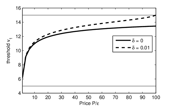
Figure 3 plots the threshold as a function of the price, of the priority queue. Observe that increases with This is intuitive because the incentive to join the high priority queue is diminished as the price increases. In fact, for we find that when However, this is not true when in which case keeps increasing to but is never equal to it. Investigating this further, since is the number of customers joining Queue revenue earned by the server would be This is not a linear function of as and depends on

In Figure 4, we plot the revenue (normalized by ) as a function of the price (normalized by ). For we observe that the revenue keeps increasing as is increased, while for there is an optimal choice of at which the revenue attains its maximum. Note that (resp. ) corresponds to the case when (resp. ). Hence, the intuition is that when there are always customers (close to customers of type ) who do not value money much. Therefore, the service provider can always increase her revenue by setting a higher price for the priority queue. On the contrary, when there exists a price large enough, that customers of type cannot afford. The latter decide to join Queue
In the previous discussions, we have considered that decreases more rapidly for smaller than it does for larger Now consider a system where decreases linearly, i.e.,
| (20) |
We now investigate the two-queue boarding game with as above, and and customer types uniformly distributed over For this system is
For to be bounded we require in which case This upper bound is achieved when As observed previously, if is sufficiently large then for (A2) it is sufficient if Further, for to be bounded, we require The thresholds and revenue behave as in the previous example
5 Revenue Maximization
In the previous section, the admission price to each of the queues was assumed given and we provided a complete characterization of the NE strategy. In this section, we investigate how the service provider can maximize its revenue by appropriately setting the prices Our motivational setting is the airplane boarding system where customers have already purchased their tickets. Hence it is reasonable to assume that there is one queue, the lowest priority queue, where there is no premium, i.e., Thus although the customers cannot balk, the existence of the a ‘free queue’ ensures that the revenue is not an increasing function of the premiums in the higher priority queues and there will be an optimum value for these prices. Further, increased service differentiation allows for increased revenues. In this section we first determine the optimum prices for a given and then numerically analyze the effect of increasing
For the queue system, is the fraction of customers that joined Queue and, hence, is the total number of customers that join Queue The revenue earned by the service provider is given by
| (21) |
We know that, at NE, Also, (18) gives a bijective relation between and Using these, we can express revenue as follows:
| (22) |
where
| (23) |
This is derived in Appendix G.
Thus, maximizing can be solved as a finite horizon dynamic program (FHDP). Notice that the first term in the expansion depends only on (action at time in the FHDP), the second term depends only on and (action and state of the system at time ), the third term depends only on and (action and state of the system at time ), and so on. We assume that the FHDP has a solution and verify this numerically.
| L | ||||||
|---|---|---|---|---|---|---|
| 2 | - | - | - | - | ||
| 3 | - | - | ||||
| 4 |
We now numerically evaluate the revenue maximizing prices by solving the FHDP. As before, and type is uniformly distributed. There are queues, and is as in (19) with
Table 1 lists the revenue maximizing prices and thresholds when and for and We observe that as the number of queues is increased, for maximum revenue, has to be decreased at each Queue This has been consistently observed for other system parameters.
| Population | Revenue | ||
|---|---|---|---|
| distribution | |||
In Table 2, we compare the maximum revenue for three different type distributions when and We observe that the revenue increases as more queues are added, regardless of the underlying type distribution. Most importantly, the increase in this revenue from three queues to four queues is as small as and for the type distributions and respectively. However, for the same type distributions the increase in maximum revenue is and respectively. This tells us that having three, may be even just two, queues shall get us very nearly the maximum revenue.
We also remark here that this observation of a small number of classes yielding nearly the maximum revenue is also seen in other similar settings that serve a heterogenous population. For example, in [20], the authors consider dividing link capacity into multiple classes of service, each with its own price, an instance of Paris Metro pricing. Utility maximising users choose the class of service and it is shown that for a large range of utility functions, the loss of revenue is small even with a small number of service classes.
Another observation from the results of Table 2 is that the revenue is larger when the type distribution is Numerically, it is consistently observed that if then the boarding game with types in yields greater maximum revenue than with a larger diversity of types provides a larger revenue. This property is known in the pricing literature, e.g., [3]. Larger diversity provides for more customers with higher valuations for quality of service (QoS). Such a user population allows the service provider to extract more consumer surplus by tuning service quality and price to each type to maximise profit.
6 Concluding Discussion
The system that we have introduced in this paper can be seen to belong to a class of queueing systems where the arrival times are endogenously determined by the customers; unlike the exogenously determined arrival times in traditional queueing systems. Clearly, there are several potential applications for systems with endogenous arrivals in modeling waiting systems at airports, bus and train terminals, concert halls, etc. A better understanding of these systems can help in a more informed sizing of waiting facilities.
Several extensions are possible. An extension of immediate interest is to develop a learning algorithm to obtain the revenue maximizing prices. Specifically, since such a game would be played out repeatedly, the outcome of each instance may be used to adapt the prices to maximize the revenue. A second extension would be to allow customers to balk if the cost is higher than the value of obtaining service.
Appendix A Proof of Lemma 1
The proof uses the optimality of and for and respectively, and the structure of the cost function.
Similarly, we can get
Adding the two we obtain
Note that as is a strictly increasing function. Therefore,
This implies that as is a strictly increasing function.
Appendix B Proof of Theorem 3.1
First note that This is derived using (2) as follows.
| (24) |
because is a non-atomic distribution, and the second equality follows from Lemma 1.
Now, since is a NE, by first order condition on (7), we have
| (25) |
where denotes derivative with respect to Differentiating (24) with respect to we get
| (26) |
Substituting (26) in (25), we obtain
Integrating both sides with respect to we get
| (27) |
This implies
| (28) |
Note that is a non-increasing function. Thus, users of type arrive last in the queue. If then the cost for user of type can be reduced by decreasing to , which contradicts the definition of . Therefore, . This implies that due to assumptions on . (28) then implies the result.
Appendix C Proof of Lemma 2
For notational simplicity, we shall denote to mean
| (29) |
in this section. Thus, the cost of a customer is given by
| (30) |
Comparing the costs of customer and we have
| (31) |
Substituting in (31), we obtain
| (32) |
The last inequality follows because minimizes Similarly, substituting in (31) we get
| (33) |
Since, we obtain
| (34) |
Adding the two inequalities, namely, (32) and (34), we get
| (35) |
Since, is an increasing function of (35) reduces to which is nothing but
as is an increasing function. Thus, is a decreasing function in
Appendix D Proof of Lemma 3
By Definition 2,
| (36) |
where the last equality follows due to Lemma 2. Now define
| (37) |
Then, we have also note that for every Differentiating this w.r.t. we obtain
| (38) |
Also, the first order derivative condition for the optimality of namely, gives
| (39) |
Substituting (38) in (39), we get
| (40) |
This can be simplified to
| (41) |
where, while the second inequality follows from the first equality uses (13) and the same arguments that are used in Appendix B to arrive at the explicit expression of
Appendix E Proof of Theorem 4.1
For the ease of presentation, we denote
| (42) |
In the following lemma, we prove that increases, while decreases in
Lemma 4
strictly increases and strictly decreases in
Proof
The optimal cost to join Queue is given by
At
where the last equality follows from (14). We therefore have
| (43) |
where the last inequality follows from Lemma 3 and the fact that is an increasing function. Using the fact that is a decreasing function and from (A1), we have
Using this in (43) gives
where the last inequality follows from (A2).
We now prove some properties of the optimal costs which help us in arriving at the thresholds.
Lemma 5
For the optimal costs, s, the following is true
- 1.
- 2.
For all we have
- 3.
There exists a unique point for every at which the two costs, namely, and intersect. Also,
Proof
Taking the derivative of w.r.t. we get
| (45) |
Using the first order optimality condition for which is
| (46) |
in (45) we get
| (47) |
For since we have
| (48) |
which follows from the fact that is an increasing function in and always positive.
Now, for using Lemma 3 in (47) and the fact that is an increasing function, we get
| (49) |
where the last inequality follows from the fact that and (A2): since implies
Analyzing the difference between and we obtain
| (50) |
where the last inequality follows from (A2), while the third in the third step we use Lemma 3 and the property that is increasing. This proves part and of the Lemma.
For part take and in First note that and from Lemma 4. Since, is continuous and there exists exactly one at which the two functions, namely, and meet. Further, note that because and, similarly, because by Lemma 4.
It only remains to show that Using part and of the Lemma it is clear that for we have and for we have Now, if then for all and hence for all Thus, over the interval we shall have and over the interval we shall have This implies that no customer will join Queue contradicting (A3). ∎
We now prove that joining Queue is the best strategy for all For this, it needs to be verified that for for all The following lemma provides some sufficient conditions for it. We later show that the optimal cost functions satisfy these sufficient conditions.
Lemma 6
If
| (51) |
and
| (52) |
then for for all
Proof
We now show, by using Lemma 5, that the conditions of Lemma 6 are indeed satisfied and, thus, it is true that for for all
- 1.
- 2.
This proves all the conditions of Lemma 6.
Appendix F Proof of Theorem 4.2
Take then
| (61) |
where the second equality follows from Lemma 2 and Theorem 4.1. Differentiating (61) w.r.t. we get
| (62) |
For optimality, must also satisfy the first order condition, namely, This gives
| (63) |
Substituting (62) in (63), we get
This gives
where is the integration constant that can be shown to equal using the same line of arguments as in Appendix B while deriving in explicit form.
Further, since is a decreasing function by Lemma 2, for all Hence, for
| (64) |
Also, note that at Queue arrival of customer is the earliest. Thus, Now, since is an increasing function for all Thus, any customer in order to minimize her waiting cost has to choose This proves the first part of Theorem 4.2 which characterizes completely. Notice that, we have also shown that satisfies
| (65) |
Appendix G Derivation of the Revenue Function
We can re-write (18) as
| (67) |
for all Adding (67) for all to we get
| (68) |
We use to denote the price vector Revenue function can be expanded as
| (69) |
Substituting (67) and (68), we obtain
| (70) |
which can be written as
| (71) |
This can be simplified as
| (72) |
Note that the first term in the second sum is Hence, by increasing index of the second summation this can be re-written as
| (73) |
This is noting but
References
- [1] P. Afeche and H. Mendelson. Pricing and priority auctions in queueing systems with a generalized delay cost structure. Management Science, 50(7), July 2004.
- [2] K. R. Balachandran. Purchasing priorities in queues. Management Science, 18(5):319–326, 1972.
- [3] C. Courcoubetis and R. Weber Pricing Communication Networks: Economics, Technology and Modeling John Wiley and Sons, 2003.
- [4] S. Doroudi, M. Akan, M. Harchol-Balter, J. Karp, C. Borgs, and J. T. Chayes. Priority pricing in queues with a continuous distribution of customer valuations. Technical Report CM-CS-13-109, Computer Science Department, Carnegie Mellon University, May 2013.
- [5] A. Glazer and R. Hassin. Stable priority purchasing in queues. Operations Research Letters, 4(6):285–288, April 1986.
- [6] O. Gueant, J. M. Lasry, and P. L. Lions. Mean field games and applications. Springer: Paris-Princeton Lectures on Mathematical Finance, 2010.
- [7] H. Honnappa and R. Jain. Strategic arrivals into queueing networks: The network concert queueing game. arXiv:1112.3052, Dec. 2011.
- [8] R. Jain, S. Juneja, and N. Shimkin. The concert queuing problem: To wait or to be late. Discrete Events Dynamic Systems, 21(1):103–138, Mar. 2011.
- [9] S. Juneja, T. Raheja, and N. Shimkin. The concert queueing game with a random volume of arrivals. In Proc. VALUETOOLS, pages 317–325, Oct. 2012.
- [10] S. Juneja and N. Shimkin. The concert queueing game: strategic arrivals with waiting and tardiness costs. Queueing Syst., 74(4):369–402, Aug. 2013.
- [11] M. A. Khan, K. P. Rath, and Y. Sun. On the existence of pure strategy equilibria in games with a continuum of players. Journal of Economic Theory, 76(1):13–46, Sep. 1997.
- [12] T. Kittsteiner and B. Moldovanu. Priority auctions and queue disciplines that depend on processing time. Management Science, 51(2):236–248, 2005.
- [13] L. Kleinrock. Optimal bribing for queue position. Operation Research, 15, 1967.
- [14] M. Lariviere and J. A. Van Mieghem, ‘ Strategically seeking service: How competition can generate Poisson arrivals Manufacturing & Service Operations Management, 6(1), Winter 2004, pp.23–40.
- [15] F. Lui. An equilibrium model of bribery. Political Economy, 93, 1985.
- [16] M. Marchand. Priority pricing. Management Science, 20(7):1131–1140, 1974.
- [17] A. Mas-Colell. On a theorem of Schmeidler. Journal of Mathematical Economics, 13(3):201–206, Dec. 1984.
- [18] A. W. Matyszkiel. Existence of pure equilibria in games with nonatomic space of players. Topological Methods in Nonlinear Analysis, 16(2):339–349, Dec. 2000.
- [19] S. Rao and E. Petersen. Optimal pricing of priority services. Operations Research, 46(1):46–56, 1998.
- [20] S. Shakkottai, R. Srikant, A. Ozdaglar, and D. Acemoglu, The Price of Simplicity. IEEE Journal on Selected Areas in Communication, vol. 26, no. 7, Sept 2008.