Constant-roll Inflation in Gravity
Abstract
We propose the study of constant-roll inflation in gravity. We use two different approaches, one that relates an gravity to well known scalar models of constant-roll and a second that examines directly the constant-roll condition in gravity. With regards to the first approach, by using well known techniques, we find the gravity which realizes a given constant-roll evolution in the scalar-tensor theory. We also perform a conformal transformation in the resulting gravity and we find the Einstein frame counterpart theory. As we demonstrate, the resulting scalar potential is different in comparison to the original scalar constant-roll case, and the same applies for the corresponding observational indices. Moreover, we discuss how cosmological evolutions that can realize constant-roll to constant-roll eras transitions in the scalar-tensor description, can be realized by vacuum gravity. With regards to the second approach, we examine directly the effects of the constant-roll condition on the inflationary dynamics of vacuum gravity. We present in detail the formalism of constant-roll gravity inflationary dynamics and we discuss how the inflationary indices become in this case. We use two well known gravities in order to illustrate our findings, the model and a power-law gravity in vacuum. As we demonstrate, in both cases the parameter space is enlarged in comparison to the slow-roll counterparts of the models, and in effect, the models can also be compatible with the observational data. Finally, we briefly address the graceful exit issue.
pacs
04.50.Kd, 95.36.+x, 98.80.-k, 98.80.Cq,11.25.-wI Introduction
The inflationary paradigm is one of the most widely accepted scenarios that describes the early Universe evolution. Traditionally, the description of the inflationary era is given in terms of a slow-rolling single scalar field, and many reviews already exist in the literature that describe the single scalar inflation [1, 2, 3]. The observational data coming from Planck 2015 [4] restricted quite significantly the single scalar field inflationary models, and many models were rendered non-viable [5]. However some single scalar models remained viable after the Planck constraints were imposed on them, and actually these models have quite appealing properties, such as the Starobinsky model [6, 7], the Higgs model [8], and a wide class of models called -attractors [9, 10, 11], see also [12, 13] for the gravity realization of -attractors.
Despite of the appealing properties of the single scalar field models of inflation, these models have a potential drawback related to non-Gaussianities [14]. Particularly, up to date the modes of the spectrum of the primordial curvature perturbations are assumed to be uncorrelated, so the spectrum is assumed to obey a Gaussian distribution. However, if non-Gaussianities are observed in the future, then the single scalar field models will be put into question since these do not predict any non-Gaussianities. One conceptually appealing way to introduce non-Gaussianities in single scalar field models is to directly modify the slow-roll condition. This approach was used in Refs. [15, 16, 17, 18, 19, 20, 21, 22, 23, 24, 25, 26, 27, 28, 29], see also [30, 31] for an alternative viewpoint. The models used in Refs. [15, 16, 17, 18, 19, 20, 21, 22, 23, 24, 25, 26, 27, 28, 29] are known as constant-roll models, and in all the cases the slow-roll era is modified. In effect, a non-zero amount of non-Gaussianities may appear in the primordial power spectrum [19, 20].
In this paper we aim to find the gravity description (for reviews on gravity see [32, 33, 34, 35, 36, 37]) of the models of constant-roll evolution. Our approach is two-fold, since firstly we shall realize the Hubble rate of some constant-roll models by using a vacuum gravity. After finding the gravity, we shall perform a conformal transformation in order to obtain the Einstein frame theory, and as we show, the obtained Einstein frame theory is different in comparison to the constant-roll models. However, it is possible to obtain concordance with the observations even for the obtained Einstein frame theories, and we calculate the spectral index and the scalar-to-tensor ratio. Also we briefly investigate which gravity can realize a model which is known to generate transitions between constant-roll eras in the Einstein frame. This difference between the Einstein frame and the gravity was also noticed in the literature, see for example [39, 40, 41, 42]. Our second approach to the constant-roll problem in the context of gravity is more direct in comparison to our first approach, since we shall find the implications of the constant-roll condition directly in the gravity theory, without invoking the scalar-tensor theories and their Hubble rate. This approach is more direct for the reason that the implications of the constant-roll condition can be seen in detail in the qualitative features of the gravity. Particularly, we shall investigate how the constant-roll condition affects the inflationary indices used for the study of inflation, and we also calculate the spectral index of primordial curvature perturbations and the scalar-to-tensor ratio. In order to demonstrate the implications of the constant-roll condition in gravity, we shall use two well-known models, the model and a power-law gravity model. In both cases we shall make two crucial assumptions, firstly that the first slow-roll index is very small during the inflationary era, a condition that was also assumed to hold true in Ref. [20]. Secondly, we shall assume that although , the constant-roll condition holds true. As we shall demonstrate, in the case of the constant-roll model, the constant-roll condition affects the resulting qualitative features of the model, making it compatible with the 2015-Planck [4] and BICEP2/Keck-Array data [43], for a wider range of the parameter space in comparison to the ordinary model. We also discuss in brief some restrictions and drawbacks of the constant-roll approach in the case of the model, which possibly occur due to the lack of analyticity in our approach. Finally, we briefly address the graceful exit issue and we investigate which restrictions it imposes on the parameter space. We perform the same analysis for the power-law gravity model, and as we demonstrate, the constant-roll power-law gravity model can be compatible with the current observational data, in contrast to the slow-roll model which is not compatible with the observations. We need to note that in both the gravity models we shall study, if the constant-roll condition is canceled, the results of the constant-roll case coincide with the slow-roll case, a behavior possibly expected since we assumed that .
This paper is organized as follows: In section II, we present the formalism with which we will be able to find the gravity description of certain scalar-tensor constant-roll models. By using the formalism, we shall realize a particularly interesting scenario of constant-roll inflation. Also we shall find the corresponding Einstein frame picture and we shall show that concordance with the observations may be achieved. In addition we present the gravity which realized a cosmic evolution that in the scalar field frame is known to produce transitions between constant-roll eras. In section III, we adopt a more direct approach, and we investigate the implications of the constant-roll condition in a vacuum gravity. We present the formalism of the constant-roll gravity and we find explicit expressions for the inflationary indices, by also comparing the results with the slow-roll case. In order to illustrate our findings, we present the constant-roll model, and also a well known power-law gravity model, and we discuss the implications and the shortcomings of the constant-roll approach, by also comparing the results with the slow-roll case. Finally the conclusions along with a discussion follow in the end of the paper.
Before we start our presentation, let us here briefly discuss the geometric conventions we shall assume to hold true for the rest of this paper. We shall assume that the background metric is a flat Friedmann-Robertson-Walker (FRW) metric with line element,
| (1) |
where denotes as usual the scale factor. Also, we assume that the metric connection is the Levi-Civita connection, which is an affine connection which is, metric compatible, torsion-less and symmetric.
II constant-roll Inflation and Einstein Frame
The constant-roll inflation scenario was introduced as an alternative to the slow-roll scenario, with the first having the appealing feature that non-Gaussianities are generated. We shall consider one model which was introduced in Refs. [21, 23], and it was studied in the context of scalar field theory. In this paper we shall be interested in realizing the resulting cosmic evolution of the scalar model appearing in Refs. [21, 23], in the context of gravity, and we explicitly construct a model which realizes the constant-roll inflation model. As it is well-known, by using a conformal transformation, the action of the gravity can be rewritten as a scalar-tensor theory. As we demonstrate, the gravity which realizes the model of constant-roll when it is conformally transformed in the Einstein frame, the resulting scalar-tensor theory is different from that used in [21, 23]. The spectral index of primordial curvature perturbations and the scalar-to-tensor ratio can be calculated by using the resulting Einstein frame theory. According to the cosmological observations, these quantities can be obtained from the correlation function of the density with respect to the angle. The angle is unaffected by the conformal transformation, and the amplitude is changed by a factor which does not depend on the spacial coordinates if we consider isotropic background. This indicates that the quantities could be obtained by using the potential in the scalar-tensor theory obtained from the gravity theory. These quantities should be different from those obtained in [21, 23] since the potentials in the scalar-tensor theory obtained from the gravity are different from the ones corresponding to the scalar-tensor theory [21, 23].
We begin by considering the general solution for the constant-roll condition in the context of scalar-tensor theory,
| (2) |
By using the FRW equations,
| (3) |
we obtain,
| (4) |
Then we acquire,
| (5) |
By eliminating and by using Eqs. (2), (4), (5) we obtain,
| (6) |
which can be integrated as follows,
| (7) |
We may furthermore rewrite Eq. (7) in the following form,
| (8) |
When , the solution of (8) is given by,
| (9) |
On the other hand, if , we find
| (10) |
where , , , and are arbitrary constants.
In the following, we consider the following cosmological evolution which was introduced in Refs. [21, 23],
| (11) |
In order to construct the gravity model which reproduces Eq. (11), we rewrite the action of the gravity as follows, [38],
| (12) |
By varying the action (12) with respect to the auxiliary scalar field , we obtain the equation,
| (13) |
which can be solved with respect as a function of the scalar curvature as . Then by substituting in the initial action, we obtain the gravity whose Lagrangian density is given by
| (14) |
Since we can redefine the scalar field freely, we may identify the scalar field with the time coordinate , . By neglecting the contribution from matter fluids, that is, we are interested in the vacuum gravity case, we obtain the following equations,
| (15) |
or equivalently,
| (16) |
If we assume that,
| (17) |
where and are constant parameters, Eq. (16) yields the following three algebraic equations,
| (18) |
For general , the above equations have no solution but if we choose to take specific values, we find the following solutions,
| (19) |
In order to consider the more general case, we define a new variable as follows,
| (20) |
Then by using the following relations,
| (21) |
we can rewrite Eq. (16) as follows,
| (22) |
which is nothing but the hypergeometric differential equation and the solutions are given by the hypergeometric functions as follows,
| (23) |
Here and are constants, which can depend on , and also
| (24) |
Since the following holds true,
| (25) |
by using Eqs. (15) and (20), we find,
| (26) |
We are interested in the case that is of the order and does not take large values. By taking this limit, we find that,
| (27) |
and therefore we get,
| (28) |
Accordingly we find,
| (29) |
We now consider the conformal transformation,
| (30) |
and we rewrite the action (12) as follows,
| (31) |
The time evolution appearing in Eq. (11) can be realized by the Einstein frame scalar-tensor theory. The potential in the scalar tensor theory in Eq. (31) is different from that in [21, 23]. Then there might be a difference in the resulting spectral index of primordial curvature perturbations and the scalar-to-tensor ratio .
We may define the slow-roll parameters in the Einstein frame as follows,
| (32) |
By using the slow-roll indexes and , we can express the observational indices and as follows,
| (33) |
Then by setting in Eqs. (28) and (29), in the limit , we get,
| (34) |
which seems too large compared with the observational data. On the other hand, by setting in Eqs. (28) and (29), we obtain,
| (35) |
We should note that both the models obtained in the cases and yield the same background cosmological evolution, but the resulting observational indices are different from each other. It is possible though to adjust the coefficients and in such a way so that these depend on . In this way we may obtain a variety of and .
It is also possible to realize cosmological models that in the scalar-tensor frame allow transitions between constant-roll eras, which correspond to different parameters . Since we identified the scalar field with the cosmological time, the model describing the transition between constant-roll eras can be realized by allowing the parameter to depend on , as follows,
| (36) |
Then, we may choose,
| (37) |
where, , , , and are constants. Then in the case , the constant-roll era with is realized, and if , the constant-roll era with is realized. The corresponding gravities can easily be found, but we omit the result for brevity, since it is too lengthy to be presented here.
We should note that even if we replace in (15) with , which is a function of the scalar field , the expressions in (36) are not the solution of the obtained equation. As we see in Eq. (37), however, we have chosen so that becomes a constant in the limits of . In the limits, the scalar field can be identified with the time coordinate although we cannot identify it as the time coordinate for finite . In the limits,the expressions in (36) satisfy (15) asymptotically and the model given in (36) really connects two different ’s.
Another interesting scenario which realizes a transition between constant-roll eras can be shown [29], that has the following canonical scalar field potential,
| (38) |
in which case the resulting Hubble evolution is,
| (39) |
and also the transition is ensured by the condition that the second slow-roll index satisfies,
| (40) |
The qualitative study of this constant-roll to constant-roll transition scenario can be found in Ref. [29]. Here we shall investigate how the evolution (39) can be realized by using a vacuum gravity and we shall mainly be interested in the Einstein frame theory corresponding to the gravity. As we shall show, the resulting Einstein frame potential is not identical to the one appearing in Eq. (38). By using the formalism we presented earlier in this section, it can easily be found that the function is equal to
| (41) |
where is the confluent hypergeometric function and is the generalized Laguerre polynomial, and , are integration constants. By using Eq. (15), the function can also be found and it is equal to,
| (42) |
Having the functions and at hand, we can use Eqs. (30) and (31) to find the potential . However, the function is not so easy to find. Therefore, in order to have an idea how the Einstein frame potential looks like, we perform an asymptotic expansion of the function for small values of , and we get at leading order,
| (43) |
where the constant parameters and are,
| (44) |
Then, the function reads,
| (45) |
hence the potential can be found by combining Eqs. (15), (30), (31), and (43), and it reads,
| (46) |
By comparing Eqs. (38) and (46), it can be seen that the scalar potentials are totally different, and the same applies even if we take the small limit of the potential (38). It is conceivable then that the potential (46) describes an entirely different cosmological evolution, and also it is not certain that the constant-roll condition still holds true. However we refer from discussing in detail these issues here.
III The Constant-roll Inflation Condition with Gravity
In the previous section our approach to the constant-roll inflationary scenarios was in some way indirect since we realized the Hubble rate corresponding to the scalar-tensor frame theories, by using gravity. In the present section we shall use the constant-roll condition directly in the gravity theory and we shall discuss the new qualitative features that the constant-roll condition imposes in the gravity inflationary phenomenology. We will be interested in two vacuum gravity models, the model and a power-law gravity model.
III.1 General Formalism of the Constant-Roll Inflation with Gravity
First let us recall here that the constant-roll inflation condition has the following form in terms of the Hubble rate,
| (47) |
where is a real parameter. In this section we shall present the theoretical framework of the gravity inflation, with the assumption that the above condition holds true. We shall assume that the physical evolution is controlled by a vacuum gravity with action,
| (48) |
where stands for the determinant of the background metric, which shall be assumed to be a flat FRW metric. By varying the action (48) with respect to the metric, we obtain the following equations of motion,
| (49) | ||||
| (50) |
where and the “dot” indicates differentiation with respect to the cosmic time. The inflationary dynamics in the context of modified gravity are well described in Refs. [44, 45, 46], see also Refs. [47, 48, 49] for some recent works. The inflationary dynamics are perfectly described by the following inflationary indices, which for a general gravity are equal to,
| (51) |
where the function appearing in Eq. (51) stands for,
| (52) |
Another useful quantity which we shall now introduce is the function , which is,
| (53) |
which we shall use later on when we calculate the scalar-to-tensor ratio.
We will be mainly interested in the calculation of the spectral index of the primordial curvature perturbations and of the scalar-to-tensor ratio in the context of pure gravity. With regard to the spectral index, in the case that , it is equal to [44, 45, 46],
| (54) |
where is equal to,
| (55) |
In the case that , the spectral index can be approximated as follows,
| (56) |
Now we turn our focus on the scalar-to-tensor ratio, which in the case of gravity is defined as follows,
| (57) |
where is defined in Eq. (53). After some algebra, it can be shown that in the case of gravity, the scalar-to-tensor ratio reads,
| (58) |
At this point we shall investigate how the inflationary indices and also the observational indices are affected by the constant-roll condition. It can be shown after some algebra that the inflationary indices (51) become,
| (59) |
where and . By imposing the condition (47), it can be shown that the following approximations hold true,
| (60) | ||||
| (61) |
Depending on the functional form of the gravity, the inflationary indices , and the corresponding observational indices and , can take various forms, so this is the subject of this section. We need to note however that the in the limit , the constant-roll and the slow-roll expressions should definitely coincide.
Before we proceed to the models we would like to note that we shall assume that the parameter still satisfies , an assumption also made in [20].
III.2 The Starobinsky Model with Constant-Roll Inflation Condition
In this section we shall investigate the theoretical implications of the constant-roll condition on the inflationary phenomenology of the inflation model, in which case the gravity is of the form [6],
| (62) |
where is a phenomenological parameter which has dimensions of mass2 and it is assumed to be quite large . For the model (62) it can be easily shown that the inflationary indices of Eq. (59) become,
| (63) |
Due to the fact that we assumed , we approximately have , therefore we can use the relation (56) for the spectral index. In addition, the scalar-to-tensor ratio can be calculated by using Eq. (58). In order to calculate the inflationary indices, we need to have an approximate expression for the Hubble rate during the era for which , with the constant-roll condition (47) approximately holding true. Hence we will solve the equations of motion (49) and (50), for the gravity (62) by using the constant-roll condition . During the era for which , or equivalently when the condition holds true, the equations of motion (49) and (50) become,
| (64) |
By using the constant-roll condition , the first differential equation in (64) becomes,
| (65) |
and since , by eliminating the dependence in the differential equation (65), we find the approximate solution,
| (66) |
where is arithmetically of the order , but with different dimensions, and also the parameter is,
| (67) |
In addition, the time instance is the horizon crossing time instance. The cosmological evolution (66) is a quasi-de Sitter evolution, a bit different from the ordinary model, however in the limit , these two coincide. In the following we shall be interested in finding the inflationary dynamics of the approximate quasi-de Sitter solution (66). The inflationary era will eventually stop if the first slow-roll index becomes of the order , so by assuming that this occurs at a time instance , with , the condition yields, . Then we obtain,
| (68) |
and by substituting we get,
| (69) |
During the era , the parameters take large values, so by omitting the last term in (69) we obtain,
| (70) |
It is worth invoking the -foldings number in the calculation, which is defined as,
| (71) |
By substituting the Hubble rate (66) in the -foldings number (71) we get,
| (72) |
so by substituting Eq. (70), we obtain,
| (73) |
Hence at leading order we have approximately,
| (74) |
Having the above relations at hand we can calculate the inflationary indices (63) and the observational indices (56) and (58). Hence, by calculating the spectral index we obtain at leading order for large-,
| (75) |
Accordingly, the scalar-to-tensor ratio at leading order is,
| (76) |
For the ordinary model, the observational indices are,
| (77) |
and by comparing Eqs. (75) and (76) with (77), it can easily be seen that in the limit , these coincide. Let us now investigate the viability of the constant-roll model by comparing the observational indices with the Planck data [4] and also with the BICEP2/Keck-Array data [43], for specific values of and . The constraints on the spectral index and on the scalar-to-tensor ratio imposed by the Planck data, are as follows,
| (78) |
and also the BICEP2/Keck-Array data [43] constraints the scalar-to-tensor ratio even further, in the following way,
| (79) |
at confidence level. Let us now investigate in some detail the parameter space of the constant-roll Starobinsky model quantified by the parameters . An analysis immediately reveals that the compatibility with the observational data can be achieved for a wide range of values for the parameters, and we now try to demonstrate this by using some illustrative plots. Firstly let us comment that the spectral index is considered within the observational constraints if it takes values in the interval , so we take this into account in our analysis.
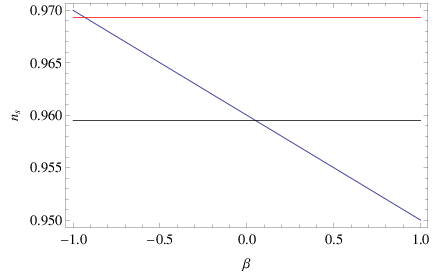
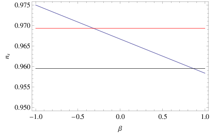
In Fig. 1 we plotted the dependence of the spectral index for (left plot) and for (right plot). In both plots, the upper (red) and lower (black) straight lines correspond to the values and respectively. As it can be seen, there is a large range of values for the parameter , for which the spectral index becomes compatible with observations and this can be achieved for various values of the -foldings number. Let us here present some characteristic examples, starting with the set of values , with the constant-roll scenario being known in the literature as ultra-slow-roll scenario [20]. For we obtain,
| (80) |
which are both within the Planck and BICEP2/Keck-Array data constraints, however this scenario is not so appealing since the -foldings number is too small. Also for we obtain,
| (81) |
which again are both within the Planck and BICEP2/Keck-Array data constraints. Another interesting constant-roll example corresponds to the value which belongs to the models studied in [23], in which case for the observational indices read,
| (82) |
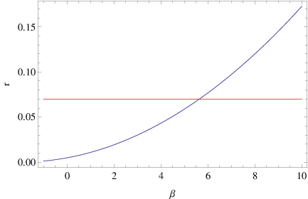
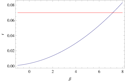
and these are observationally acceptable. From the analysis we performed it seems that both the constant-roll models with negative and positive produce viable results, at least for the Starobinsky model in vacuum. Also in Fig. 2, the scalar-to-tensor ratio is plotted as a function of for (left plot), and for (right plot) with the red line indicating the BICEP2/Keck-Array constraint . As it can be seen, there is a large range of values for which the resulting scalar-to-tensor ratio is in concordance with the observational data.
Before closing this section we discuss two issues related to the horizon crossing and the end of inflation. For the derivation of the observational indices, we calculated the inflationary indices at the horizon crossing, and hence the same applies for the observational indices. While this is not necessarily the case in the scalar-tensor description as it can be seen in Ref. [20], in our case, since all the inflationary indices are quite small when , the calculation can be performed at the horizon crossing. Also we assumed that inflation ends when , however this can be questionable. Traditionally, when , the slow-roll era ends, and this is usually identified with the end of the inflationary era. However, the actual ending of inflation is caused by growing curvature perturbations which render the final de Sitter attractor unstable. In our case the final attractor is a quasi-de Sitter attractor and since we are dealing with an model, the term is known to produce the exit from inflation [50], due to growing curvature perturbations. It is worth briefly discussing this issue at this point, so let us consider how the perturbations from the de Sitter solution grow as a function of the cosmic-time. This might eventually impose some restrictions on the parameter . Consider the following perturbation of the de Sitter solution,
| (83) |
so we substitute (83) in Eq. (49), and by keeping linear terms of the function , and also by using the constant-roll condition (47), we obtain the following differential equation,
| (84) |
The differential equation (84) determines the evolution of linear perturbations of the de Sitter solution, and it can be solved analytically, with the solution being,
| (85) |
where is an integration constant. From the above solution, since , in order to have growing perturbations, the parameter must satisfy . However this restriction leads to a rather questionable result, since for , the -foldings number must be much smaller than in order to obtain compatibility with the observational data. This means that the constant-roll scenario lasts only -foldings, which is a relatively small period. This is possibly an indication that for , the constant-roll scenario becomes quite unstable, however this needs to be further investigated, since the approach we adopted is based on keeping linear perturbation terms, hence our results might be an artifact of the linear perturbation theory.
III.3 Power-law Gravity Model with Constant-Roll Inflation Condition
Now let us consider another interesting gravity model, in which case the has the following form,
| (86) |
where the parameters and are positive numbers. By taking into account the constant-roll condition (47), the inflationary indices of Eq. (59) take the following form,
| (87) |
It can be easily confirmed by looking the related literature that the expressions above coincide with the ordinary power-law gravity model when . In order to proceed and further demonstrate this coincidence for , we will calculate the approximate form of the Hubble rate by using the gravity equations of motion. Particularly, the differential equation (49) when , it takes the following approximate form,
| (88) |
and by analytically solving this equation we obtain the following solution,
| (89) |
which for coincides with the well known solution corresponding to the ordinary slow-roll power-law gravity model.
We proceed to the calculation of the inflationary indices by taking into account the solution (89), and these become,
| (90) |
By comparing the above indices with the ones in the literature for the power-law gravity model (86), it can be seen that these coincide for . In order to calculate the spectral index, due to the fact that the condition does not necessarily hold true, we need to use Eq. (54) and find the explicit form of . By substituting the inflationary indices from Eq. (90) to Eq. (55), the function reads,
| (91) |
and by substituting Eq. (91) in Eq. (54), the spectral index reads,
| (92) |
Accordingly, by substituting the analytic form of from Eq. (90) in Eq. (58), we can obtain the scalar-to-tensor ratio, which is,
| (93) |
It can be crosschecked with the related literature that the expressions (92) and (93) coincide with the standard results for the observational indices corresponding with the slow-roll power-law gravity model, when . Let us investigate whether the constant-roll power-law gravity model is viable or not and we compare the results with the slow-roll power law power-law gravity model. With regards to the latter, the observational indices are identical to the ones appearing in Eqs. (92) and (93) for and only for the spectral index is in concordance with the Planck data (78), but the scalar-to-tensor ratio is so it is excluded. Let us now see what happens in the constant-roll case, for which enters the equations, so now we investigate the parameter space of the model which is governed by the parameters . In this case, the analysis shows that the compatibility with observational data can be achieved for a wide range of values of the parameters. Recall that the spectral index is considered within the observationally acceptable if it takes values in the interval and also the scalar-to-tensor ratio must satisfy .
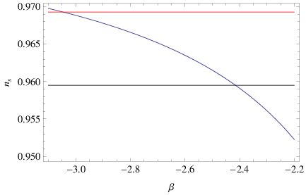
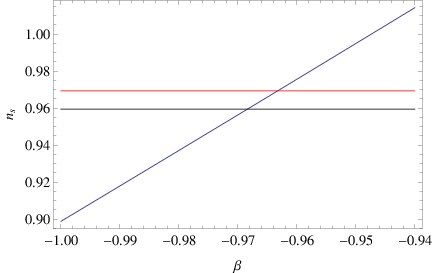
In Fig. 3 we plotted the dependence of the spectral index for (left plot) and for (right plot). As in the previous figures, in both plots, the upper (red) and lower (black) straight lines correspond to the values and respectively. As it can be seen, there is a large range of values for the parameter , for which the spectral index becomes compatible with observations, however the analysis of the scalar-to-tensor ratio will reveal some constraints which should be imposed on the parameter , which recall has to be positive. So it is useful to use various characteristic examples at this point. Consider the case, which corresponds to the ultra-slow-roll scenario of Ref. [20], in which case for the observational indices become,
| (94) |
and as it can be seen, the scalar-to-tensor value is excluded by both Planck and BICEP2/Keck-Array data. Consider now the set , for which the observational indices read,
| (95) |
which are both within the Planck and BICEP2/Keck-Array data constraints, however this scenario is not so appealing since it predicts an almost zero scalar-to-tensor ratio. Also for we obtain,
| (96) |
which are in good agreement with the Planck and BICEP2/Keck-Array data constraints. So far all the examples have negative , but there are cases that a positive beta yields optimal results. For example by choosing or equivalently , we obtain,
| (97) |
The above examples show that the large values for the parameter seem not to be favored, and we discuss this shortly in more detail. In order to better understand the behavior of the observational indices as functions of and , we need to provide some illustrative plots that will clearly demonstrate how the scalar-to-tensor ratio behaves. In Fig. 4, we plotted the scalar-to-tensor ratio as a function of for (left plot), and for (right plot) with the red line in both cases indicating the BICEP2/Keck-Array constraint .
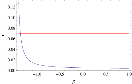
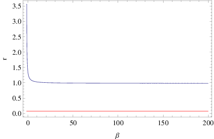
Clearly, the right plot reveals an interesting behavior, since the scalar-to-tensor ratio never becomes compatible with the BICEP2/Keck-Array constraints. Actually, it is easy to show that for , the scalar-to-tensor ratio never drops below the bound imposed by the BICEP2/Keck-Array collaboration, regardless of the value of the parameter .
Finally, let us briefly discuss the graceful exit issue, and an indication that this actually occurs is to find growing perturbation of the solution (89). So consider the following linear perturbation of the solution (89),
| (98) |
so by substituting (98) in Eq. (88), we obtain the following differential equation,
| (99) |
which can be easily solved, with the solution being,
| (100) |
where is an integration constant. Hence, the solution (100) indicates that the linear perturbations of the solution (89) decay as . Interestingly enough, the parameters and do not affect the evolution of the perturbations, at least in the context of the constant-roll approximation, since the differential equation (99) is obtained by assuming that the constant-roll condition holds true. We need to note that this result should be further investigated, since our approach was a linear perturbation approximation. We hope to address this issue further in a future work.
IV Conclusions
The aim of this paper was two-fold, firstly we investigated how scalar-tensor constant-roll cosmological evolution scenarios can be realized in the context of vacuum gravity and secondly we examined what are the implications of the constant-roll condition on gravity, without invoking the scalar-tensor solutions.
In the first approach, after we found the resulting picture, we conformally transformed the theory in order to obtain the Einstein frame scalar-tensor theory. The resulting scalar theory yields different scalar potential and observational indices in comparison to the initial scalar theory. We also found the gravity counterparts of some theories that in the scalar-tensor frame realize transitions between constant-roll eras. As in the previous case, the Einstein frame corresponding theory is very different in comparison to the initial scalar-tensor theory. The reason behind this difference between the initial scalar theory and the Einstein frame theory corresponding to the gravity, is possibly that the constant-roll condition is quite different in the Einstein frame in comparison to the gravity description. This behavior is also discussed in the literature [39, 40, 41, 42], however for conformal invariant quantities a similarity between the two frames is expected [39, 51, 52].
In the second approach we investigated the implications of the constant-roll condition on the inflationary dynamics of a vacuum gravity, without invoking the scalar-tensor theory. We presented the functional form of the inflationary indices in the constant-roll case, and we compared the results to the standard slow-roll inflationary indices. After presenting in detail the formalism of constant-roll gravity inflation, we applied our findings in two well known gravity models, the Starobinsky and the power-law gravity model. As we demonstrated, the Starobinsky model remains compatible with the observational data, even in the constant-roll case, with the difference in comparison to the ordinary slow-roll model being that the parameter space is enlarged, so there is a wide range of parameter values for which the compatibility with the data can be achieved. In the case of the power-law gravity model, the results are more interesting, since the constant-roll power-law gravity model of inflation, can be compatible with observations, in contrast to the slow-roll one. We performed a thorough analysis in which we studied in detail the behavior of the spectral index of the power-spectrum of the primordial curvature perturbations, and of the scalar-to-tensor ratio, and we examined when the compatibility with the data can be achieved.
For some future applications we shall mention here that an important study has to do with the reheating process in the context of gravity, with the constant-roll inflation governing the inflationary evolution. This is particularly interesting since it is related to the graceful exit from inflation issue. It would be interesting to investigate the implications of a constant-roll era on the reheating process. Also the issue of non-Gaussianities in the context of gravity is also important. The well-known results for non-Gaussianities that occur if the slow-roll condition is violated, should in principle hold true in the context of gravity, too, but nevertheless, this should be carefully and appropriately addressed. We hope to study some of these issues in a future work.
Also, after this paper appeared in arXiv, another paper also appeared in which the constant-roll inflation in gravity was studied [53]. The differences are profound, since in our case, the constant-roll condition in the Jordan frame is considered, which is a direct generalization of the scalar-tensor constant-roll condition. Also in [53], the gravity is not studied in the Jordan frame but in the Einstein frame, whereas in our case the second part of this paper is devoted on the Jordan frame study.
Acknowledgments
This work is supported by MINECO (Spain), project FIS2013-44881, FIS2016-76363-P and by CSIC I-LINK1019 Project (S.D.O) and by Ministry of Education and Science of Russia (S.D.O and V.K.O), and (in part) by MEXT KAKENHI Grant-in-Aid for Scientific Research on Innovative Areas “Cosmic Acceleration” (No. 15H05890) (S.N.).
References
- [1] A. D. Linde, Lect. Notes Phys. 738 (2008) 1 doi:10.1007/978-3-540-74353-8_1 [arXiv:0705.0164 [hep-th]].
- [2] D. S. Gorbunov and V. A. Rubakov,“Introduction to the theory of the early universe: Cosmological perturbations and inflationary theory,” Hackensack, USA: World Scientific (2011) 489 p
- [3] D. H. Lyth and A. Riotto, Phys. Rept. 314 (1999) 1 doi:10.1016/S0370-1573(98)00128-8 [hep-ph/9807278].
- [4] P. A. R. Ade et al. [Planck Collaboration], Astron. Astrophys. 594 (2016) A20 doi:10.1051/0004-6361/201525898 [arXiv:1502.02114 [astro-ph.CO]].
- [5] J. Martin, Class. Quant. Grav. 33 (2016) no.3, 034001. doi:10.1088/0264-9381/33/3/034001
- [6] A. A. Starobinsky, Phys. Lett. 91B (1980) 99. doi:10.1016/0370-2693(80)90670-X
- [7] J. D. Barrow and S. Cotsakis, Phys. Lett. B 214 (1988) 515. doi:10.1016/0370-2693(88)90110-4
- [8] F. L. Bezrukov and M. Shaposhnikov, Phys. Lett. B 659 (2008) 703 doi:10.1016/j.physletb.2007.11.072 [arXiv:0710.3755 [hep-th]].
- [9] R. Kallosh and A. Linde, JCAP 1307 (2013) 002 doi:10.1088/1475-7516/2013/07/002 [arXiv:1306.5220 [hep-th]].
- [10] S. Ferrara, R. Kallosh, A. Linde and M. Porrati, Phys. Rev. D 88 (2013) no.8, 085038 doi:10.1103/PhysRevD.88.085038 [arXiv:1307.7696 [hep-th]].
- [11] R. Kallosh, A. Linde and D. Roest, JHEP 1311 (2013) 198 doi:10.1007/JHEP11(2013)198 [arXiv:1311.0472 [hep-th]].
- [12] S. D. Odintsov and V. K. Oikonomou, Phys. Rev. D 94 (2016) no.12, 124026 doi:10.1103/PhysRevD.94.124026 [arXiv:1612.01126 [gr-qc]].
- [13] S. D. Odintsov and V. K. Oikonomou, arXiv:1611.00738 [gr-qc].
- [14] X. Chen, Adv. Astron. 2010 (2010) 638979 doi:10.1155/2010/638979 [arXiv:1002.1416 [astro-ph.CO]].
- [15] S. Inoue and J. Yokoyama, Phys. Lett. B 524 (2002) 15 doi:10.1016/S0370-2693(01)01369-7 [hep-ph/0104083].
- [16] N. C. Tsamis and R. P. Woodard, Phys. Rev. D 69 (2004) 084005 doi:10.1103/PhysRevD.69.084005 [astro-ph/0307463].
- [17] W. H. Kinney, Phys. Rev. D 72 (2005) 023515 doi:10.1103/PhysRevD.72.023515 [gr-qc/0503017].
- [18] K. Tzirakis and W. H. Kinney, Phys. Rev. D 75 (2007) 123510 doi:10.1103/PhysRevD.75.123510 [astro-ph/0701432].
- [19] M. H. Namjoo, H. Firouzjahi and M. Sasaki, Europhys. Lett. 101 (2013) 39001 doi:10.1209/0295-5075/101/39001 [arXiv:1210.3692 [astro-ph.CO]].
- [20] J. Martin, H. Motohashi and T. Suyama, Phys. Rev. D 87 (2013) no.2, 023514 doi:10.1103/PhysRevD.87.023514 [arXiv:1211.0083 [astro-ph.CO]].
- [21] H. Motohashi, A. A. Starobinsky and J. Yokoyama, JCAP 1509 (2015) no.09, 018 doi:10.1088/1475-7516/2015/09/018 [arXiv:1411.5021 [astro-ph.CO]].
- [22] Y. F. Cai, J. O. Gong, D. G. Wang and Z. Wang, JCAP 1610 (2016) no.10, 017 doi:10.1088/1475-7516/2016/10/017 [arXiv:1607.07872 [astro-ph.CO]].
- [23] H. Motohashi and A. A. Starobinsky, arXiv:1702.05847 [astro-ph.CO].
- [24] S. Hirano, T. Kobayashi and S. Yokoyama, Phys. Rev. D 94 (2016) no.10, 103515 doi:10.1103/PhysRevD.94.103515 [arXiv:1604.00141 [astro-ph.CO]].
- [25] L. Anguelova, Nucl. Phys. B 911 (2016) 480 doi:10.1016/j.nuclphysb.2016.08.020 [arXiv:1512.08556 [hep-th]].
- [26] J. L. Cook and L. M. Krauss, JCAP 1603 (2016) no.03, 028 doi:10.1088/1475-7516/2016/03/028 [arXiv:1508.03647 [astro-ph.CO]].
- [27] K. S. Kumar, J. Marto, P. Vargas Moniz and S. Das, JCAP 1604 (2016) no.04, 005 doi:10.1088/1475-7516/2016/04/005 [arXiv:1506.05366 [gr-qc]].
- [28] S. D. Odintsov and V. K. Oikonomou, arXiv:1703.02853 [gr-qc].
- [29] S. D. Odintsov and V. K. Oikonomou, arXiv:1704.02931 [gr-qc].
- [30] J. Lin, Q. Gao and Y. Gong, Mon. Not. Roy. Astron. Soc. 459 (2016) no.4, 4029 doi:10.1093/mnras/stw915 [arXiv:1508.07145 [gr-qc]].
- [31] Q. Gao and Y. Gong, arXiv:1703.02220 [gr-qc].
- [32] S. Nojiri and S. D. Odintsov, eConf C 0602061 (2006) 06 [Int. J. Geom. Meth. Mod. Phys. 4 (2007) 115] doi:10.1142/S0219887807001928 [hep-th/0601213].
- [33] S. Capozziello and M. De Laurentis, Phys. Rept. 509 (2011) 167 doi:10.1016/j.physrep.2011.09.003 [arXiv:1108.6266 [gr-qc]].
- [34] V. Faraoni and S. Capozziello, Fundam. Theor. Phys. 170 (2010). doi:10.1007/978-94-007-0165-6
- [35] S. Capozziello, M. De Laurentis and V. Faraoni, Open Astron. J. 3 (2010) 49 doi:10.2174/1874381101003010049, 10.2174/1874381101003020049 [arXiv:0909.4672 [gr-qc]].
- [36] S. Nojiri and S. D. Odintsov, Phys. Rept. 505 (2011) 59 doi:10.1016/j.physrep.2011.04.001 [arXiv:1011.0544 [gr-qc]].
- [37] T. Clifton, P. G. Ferreira, A. Padilla and C. Skordis, Phys. Rept. 513 (2012) 1 [arXiv:1106.2476 [astro-ph.CO]].
- [38] S. Nojiri and S. D. Odintsov, Phys. Rev. D 74 (2006) 086005 doi:10.1103/PhysRevD.74.086005 [hep-th/0608008].
- [39] G. Domenech and M. Sasaki, Int. J. Mod. Phys. D 25 (2016) no.13, 1645006 doi:10.1142/S0218271816450061 [arXiv:1602.06332 [gr-qc]].
- [40] S. Bahamonde, S. D. Odintsov, V. K. Oikonomou and P. V. Tretyakov, Phys. Lett. B 766 (2017) 225 doi:10.1016/j.physletb.2017.01.012 [arXiv:1701.02381 [gr-qc]].
- [41] S. Bahamonde, S. D. Odintsov, V. K. Oikonomou and M. Wright, Annals Phys. 373 (2016) 96 doi:10.1016/j.aop.2016.06.020 [arXiv:1603.05113 [gr-qc]].
- [42] D. J. Brooker, S. D. Odintsov and R. P. Woodard, Nucl. Phys. B 911 (2016) 318 doi:10.1016/j.nuclphysb.2016.08.010 [arXiv:1606.05879 [gr-qc]].
- [43] P. A. R. Ade et al. [BICEP2 and Keck Array Collaborations], Phys. Rev. Lett. 116 (2016) 031302 doi:10.1103/PhysRevLett.116.031302 [arXiv:1510.09217 [astro-ph.CO]].
- [44] H. Noh and J. c. Hwang, Phys. Lett. B 515 (2001) 231 [astro-ph/0107069].
- [45] J. c. Hwang and H. r. Noh, Phys. Rev. D 65 (2002) 023512 doi:10.1103/PhysRevD.65.023512 [astro-ph/0102005].
- [46] J. c. Hwang and H. Noh, Phys. Lett. B 506 (2001) 13 doi:10.1016/S0370-2693(01)00404-X [astro-ph/0102423].
- [47] S. Nojiri, S. D. Odintsov and V. K. Oikonomou, Phys. Rev. D 94 (2016) no.10, 104050 doi:10.1103/PhysRevD.94.104050 [arXiv:1608.07806 [gr-qc]].
- [48] S. D. Odintsov and V. K. Oikonomou, Class. Quant. Grav. 33 (2016) no.12, 125029 doi:10.1088/0264-9381/33/12/125029 [arXiv:1602.03309 [gr-qc]].
- [49] S. D. Odintsov and V. K. Oikonomou, Phys. Rev. D 92 (2015) no.12, 124024 doi:10.1103/PhysRevD.92.124024 [arXiv:1510.04333 [gr-qc]].
- [50] K. Bamba, R. Myrzakulov, S. D. Odintsov and L. Sebastiani, Phys. Rev. D 90 (2014) no.4, 043505 doi:10.1103/PhysRevD.90.043505 [arXiv:1403.6649 [hep-th]].
- [51] D. I. Kaiser, [astro-ph/9507048].
- [52] V. Faraoni, Phys. Rev. D 75 (2007) 067302 doi:10.1103/PhysRevD.75.067302 [gr-qc/0703044 [GR-QC]].
- [53] H. Motohashi and A. A. Starobinsky, Eur. Phys. J. C 77 (2017) no.8, 538 doi:10.1140/epjc/s10052-017-5109-x [arXiv:1704.08188 [astro-ph.CO]].