A Novel Receiver Design with Joint Coherent and Non-Coherent Processing

Wireless communications has witnessed several major theoretical advancements in the last few decades, which have been quickly incorporated into communication standards, e.g., multiple input multiple output (MIMO) systems and orthogonal frequency division multiple access (OFDMA) [1]. The baseband receiver design, underlying these technologies, has been the receiver based on a coherent detection (CD), i.e., coherent receiver for short, which has been adopted exclusively in nearly all the popular wireless communication standards. The coherent receiver design has stayed virtually unchanged throughout the evolution of wireless communication systems to date.

The recent trend towards a large number of antennas at the transmitter or receiver (such as in massive MIMO and millimeter wave systems [2, 3]) provides incentive to rethink the coherent receiver design for future communication systems. This is because provision of accurate channel state information (CSI) becomes challenging in scenarios with a massive number of antennas. In this regard, power/intensity-detection (PD) based non-coherent receivers have been proposed [4] and [5]. Although, in general, non-coherent receivers suffer from a performance loss compared to coherent receivers, their low cost and low power consumption makes them attractive for systems with a large number of antennas. It is proved in [4] that PD-based non-coherent modulation in a massive single input multiple output (SIMO) system can achieve a scaling law which is the same as the coherent modulation scheme with an increasing number of antennas. It is also shown in [5] that the performance of the PD-based non-coherent modulation asymptotically approaches the performance of coherent detection in high SNR regimes. These studies show that PD-based non-coherent receivers can offer a performance comparable to coherent receivers in future wireless systems.

Another motivation for considering PD-based non-coherent receivers comes from the recent interest in simultaneous wireless information and power transfer (SWIPT) [6, 7, 8, 9]. In such systems, a user is assumed to be equipped with an energy receiver which is based on non-coherent RF (radio frequency)-to-DC (direct current) conversion, and a conventional coherent (information) receiver. In SWIPT systems, the user employs the energy receiver and the coherent receiver separately: (i) In time-switching, the user switches between the two receivers, depending on whether it is in RF energy harvesting (EH) mode or information detection mode, or (ii) in power-splitting, the user splits the received signal into two streams, and then sends one stream to the energy receiver and the other to the coherent receiver.

Although the PD-based non-coherent receiver has received more attention in wireless communication systems recently, it has played an important role in optical communications for a long time. For the low-cost wireless infrared communication system [10], intensity modulation (IM) is the most commonly adopted modulation scheme. For IM-based wireless infrared communication, information is carried by the instantaneous power of the carrier, and the receiver uses a photodetector to produce a current proportional to the received instantaneous power directly, i.e., PD-based non-coherent demodulation. The wireless infrared communication channel is usually referred to as the intensity channel or the non-coherent additive white Gaussian noise (AWGN) channel, echoing the coherent AWGN channel. The modulation schemes and the capacity of the non-coherent AWGN channel were studied in [11] and [12], respectively.

Motivated by the recent interest in the PD-based non-coherent receiver, we consider a basic point-to-point communication system and revisit the design of the communication receiver. Rather than focusing on an improved design for either coherent receiver or non-coherent receiver alone, we consider a receiver with joint coherent and PD-based non-coherent processing. To the best of our knowledge, this is an open problem in the literature and it is not immediately clear whether joint processing will be better than either coherent or PD-based non-coherent processing alone. In this work, we show that it can in fact significantly improve the achievable rate and also reduce the symbol error rate (SER).

The main contributions of the paper are summarized as follows:

1. 1)

   We propose a novel information receiver architecture for a $K$-antenna receiver called splitting receiver. The received signal at each antenna is split into two streams by a passive power splitter with a certain splitting ratio. One stream is processed by a conventional (coherent) CD circuit, and the other is processed by a (non-coherent) PD circuit, and then the $2K$ streams of processed signal are jointly used for information detection.

2. 2)

   As a variant of the splitting receiver, we also propose a simplified receiver where no power splitters are required and a fixed number of antennas are connected to CD circuits and the remaining antennas are connected to PD circuits. Analytically, the simplified receiver can be treated as a special case of a splitting receiver, where the splitting ratio at each antenna can only take $1$ or $0$.

3. 3)

   We show that the splitting receiver (and also the simplified receiver), increases the dimension of the received signal space, since the noise adds linearly to the signal in the coherent receiver part and the noise adds to the squared amplitude of the signal in the PD-based non-coherent receiver part. This results in improved communication performance.

4. 4)

   From an information-theoretic perspective, we model the channel introduced by the splitting receiver as a splitting channel. Assuming a Gaussian input to the splitting channel, in the high signal-to-noise-ratio (SNR) regime, we show analytically that: (i) The asymptotic maximum mutual information of the splitting channel is $3/2$ times that of either the coherent AWGN channel or the non-coherent AWGN channel, under the same average received signal power constraint. (ii) For a splitting receiver with a single receiver antenna, the asymptotic optimal power splitting ratio is $1/3$. (iii) For the simplified receiver with a large number of receiver antennas, connecting half the antennas to the CD circuits and the other half to the PD circuits is the optimal strategy.

5. 5)

   For transmissions based on practical modulations, we analyze the symbol decision region and the symbol error rate (SER) at the splitting receiver. Considering high SNR regime, we derive the SER expression for a general modulation scheme. The analytical results show that, compared with the conventional coherent receiver, the splitting receiver achieves asymptotic SER reduction by a factor of $M-1$ for $M$-PAM (pulse amplitude modulation) and $\sqrt{M}-1$ for $M$-QAM (quadrature amplitude modulation).

This paper is organized as follows. Section II presents the system model, the proposed receiver architectures and the splitting channel. Section III analyzes the mutual information of the splitting channel with a Gaussian input. Section IV presents the received signal constellation at the splitting receiver for practical modulation schemes. Section V shows the SER results of practical modulation schemes. Finally, Section VI concludes the paper.

Notation: $\tilde{\cdot}$ denotes a complex number. $(\cdot)^{*}$ and $|\cdot|$ denote the conjugate and the absolute-value norm of a complex number, respectively. $\mathrm{Real}\{\cdot\}$ and $\mathrm{Imag}\{\cdot\}$ denotes the real part and the imaginary part of a complex number, respectively. $\mathrm{Pr}\left(\cdot\right)$ denotes the probability of an event. $h(\cdot)$, $h(\cdot,\cdot)$, $h(\cdot|\cdot)$ denote the differential entropy, joint and conditional differential entropy, respectively. $\mathcal{I}(\cdot;\cdot)$ denotes the mutual information. Random variables and their realizations are denoted by upper and lower case letters, respectively. $\mathrm{erfc}(\cdot)$ is the complementary error function, and $Q(x)\triangleq\frac{1}{2}\mathrm{erfc}(\frac{x}{\sqrt{2}})$ is the Q-function.

Splitting receiver: The proposed splitting receiver architecture is illustrated in Figs. 1(a) and (b). In the first stage, the received signal at each antenna is split into two streams by an ideal passive RF power splitter. We assume there is no power loss or noise introduced during the splitting process [13, 14, 15]. One stream is sent to the (conventional) CD circuit and the other to the PD circuit. The signals in the CD and PD circuits are first converted to the baseband signals and then sampled and digitized by the analog-to-digital converters (ADCs) accordingly, for further processing. Specifically, the rectifier-based PD circuit converts the RF signal into a DC signal with a conversion efficiency $\eta$. In the second stage, all the $2K$ streams of signal of the $K$ antennas are jointly used for information detection.¹¹ 1 Although the CD and PD circuits may have different detection sensitivity level in practice [16], we assume both the circuits are able to detect arbitrarily small power signal for tractability. Note that although we focus on the wireless communication application in this paper, the proposed splitting receiver with single-antenna ($K=1$) is also applicable to cable and fibre-optical communication systems.

Simplified receiver: We also propose a simplified receiver, as a variant of the splitting receiver, where no power splitters are required. This is illustrated in Fig. 2. In the simplified receiver, $K_{1}$ antennas ($1\leq K_{1}<K$) are connected to the CD circuit and the remaining antennas are connected to the PD circuits. This is illustrated in Fig. 2. We assume that the connections are determined offline, hence do not depend on the instantaneous channel coefficients at each antenna.

In this section, we present the signal model for the splitting receiver. Note that the simplified receiver can be analytically treated as a special case of the splitting receiver with power splitting ratios taking binary values only, i.e., $\rho_{k}\in\{0,1\}$, for all $k=1,2,...,K$.

Based on [15, 12], the output signals from the CD and PD circuits at the $k$th antenna are given by, respectively,

	$\displaystyle\tilde{Y}_{1,k}$	$\displaystyle=\sqrt{\rho_{k}\mathcal{P}}\tilde{h}_{k}\tilde{X}+\tilde{Z}_{k},$		(1)
	$\displaystyle Y_{2,k}$	$\displaystyle=\eta(1-\rho_{k})|\tilde{h}_{k}|^{2}\mathcal{P}|\tilde{X}|^{2}+N^{\prime}_{k},$		(2)

where $\rho_{k}\in\left[0,1\right]$ is the power splitting ratio. $\tilde{X}$ is the transmitted signal with normalized variance and $\tilde{X}\in\mathcal{X}$, where $\mathcal{X}$ denotes the set of all possible transmitted signals. $\tilde{Z}_{k}$ is the post-processing complex AWGN of the CD circuit with the mean of zero and the variance of $\sigma^{2}_{\mathrm{cov}}$, which includes both the RF band to baseband conversion noise and the ADC noise. $N^{\prime}_{k}$ is the post-processing noise of the PD circuit which is also assumed to be real Gaussian noise [12], which includes both the rectifier noise and the ADC noise. Note that we only consider the post-processing noise $\tilde{Z}_{k}$ and $N^{\prime}_{k}$, i.e., we ignore the pre-processing noise, such as the antenna noise which is almost at the thermal noise level and is much smaller than the post-processing noise [15].

Without loss of generality, scaling (2) by $\eta$, the received signal $Y_{2,k}$ can be rewritten as

$\displaystyle Y_{2,k}$

$\displaystyle=(1-\rho_{k})|\tilde{h}_{k}|^{2}\mathcal{P}|\tilde{X}|^{2}+{\color[rgb]{0,0,0}N_{k}},$

(3)

where $N_{k}\triangleq N^{\prime}_{k}/(\eta)$ is the equivalent rectifier conversion AWGN with the mean of zero and the variance $\sigma^{2}_{\mathrm{rec}}$.

To detect the transmitted signal $\tilde{X}$, similar with a conventional SIMO receiver, the optimal method is the maximal ratio combining (MRC). We assume that the receiver has perfect channel state information (CSI), i.e., knowledge of $\tilde{h}_{k}$. Since the $K$-antenna received signals $\tilde{Y}_{1,k}$ and $Y_{2,k}$, $k=1,2,...,K$, lie in different signal spaces, we use MRC for coherently processed signals (i.e., $\tilde{Y}_{1,k}$) and non-coherent signals (i.e., $Y_{2,k}$) separately. Based on (1) and (3), the combined coherently and non-coherently processed signals are given by, respectively,

	$\displaystyle\tilde{Y}_{1}$	$\displaystyle=\left(\sum\limits_{k=1}^{K}\rho_{k}|\tilde{h}_{k}|^{2}\right)\sqrt{\mathcal{P}}\tilde{X}+\sum\limits_{k=1}^{K}\sqrt{\rho_{k}}\tilde{h}^{*}_{k}\tilde{Z}_{k},$		(4)
	$\displaystyle Y_{2}$	$\displaystyle=\left(\sum\limits_{k=1}^{K}(1-\rho_{k})^{2}|\tilde{h}_{k}|^{4}\right)\mathcal{P}|\tilde{X}|^{2}+\sum\limits_{k=1}^{K}(1-\rho_{k})|\tilde{h}_{k}|^{2}N_{k}.$

For convenience of analysis, after linear scaling, (4) can be rewritten as

$\displaystyle\tilde{Y}_{1}$

$\displaystyle=\sqrt{\Theta_{1}}\sqrt{\mathcal{P}}\tilde{X}+\tilde{Z},\ Y_{2}=\sqrt{\Theta_{2}}\mathcal{P}|\tilde{X}|^{2}+N,$

(5)

where

$\displaystyle\Theta_{1}$

$\displaystyle={\sum\limits_{k=1}^{K}\rho_{k}|\tilde{h}_{k}|^{2}},\ \Theta_{2}={\sum\limits_{k=1}^{K}(1-\rho_{k})^{2}|\tilde{h}_{k}|^{4}},$

(6)

and $\tilde{Z}$ and $N$ follow the same distributions as $\tilde{Z}_{k}$ and $N_{k}$, respectively. The two-dimensional signal $\tilde{Y}_{1}$ and the one-dimensional signal $Y_{2}$ form a triple $(\tilde{Y}_{1},Y_{2})$, which is the equivalent received signal of the $K$-antenna splitting receiver.

It is interesting to see that since the two-dimensional signal $\tilde{Y}_{1}$ lies on the in-phase-quadrature (I-Q) plane and the one-dimensional signal $Y_{2}$ lines on the power (P)-axis, the equivalent received signal $(\tilde{Y}_{1},Y_{2})$ lies in the three-dimensional I-Q-P space. This is different from the conventional coherent (two-dimensional) and non-coherent (one-dimensional) receiver signal spaces. Thus, the splitting receiver expands the received signal space and fundamentally changes the way in which the signal is processed compared with the conventional receivers.

Considering the noiseless signal, i.e., letting $\tilde{Z}$ and $N=0$ in (5), we have $Y_{2}=\frac{\sqrt{\Theta_{2}}}{\Theta_{1}}|\tilde{Y}_{1}|^{2}$ from (5), which is a paraboloid equation. From a geometric point of view, defining $\vec{\rho}\triangleq[\rho_{1},\rho_{2},...\ \rho_{K}]$, $\vec{1}\triangleq\underbrace{[1,1,\cdots,1]}_{K}$, and $\vec{0}\triangleq\underbrace{[0,0,\cdots,0]}_{K}$, the splitting receiver is actually bending the noiseless received signal space into a paraboloid with $\vec{\rho}$ as illustrated in Fig. 3. When $\vec{\rho}=\vec{1}$, i.e., a non-splitting case, the splitting receiver degrades to the coherent receiver. As the parameter $\sqrt{\Theta_{2}}/\Theta_{1}$ increases, e.g., each element of $\vec{\rho}$ decreases, the splitting receiver bends the signal plane to a paraboloid, which is taller and thinner with a larger $\sqrt{\Theta_{2}}/\Theta_{1}$ , e.g., a smaller $\vec{\rho}$. When $\vec{\rho}=\vec{0}$, the splitting receiver degrades to the PD-based non-coherent receiver.

In this paper, PD-based non-coherent receiver is named as non-coherent receiver for short, and we refer to both the $K$-antenna coherent receiver (i.e., $\vec{\rho}=\vec{1}$) and the $K$-antenna non-coherent receiver (i.e., $\vec{\rho}=\vec{0}$) as the conventional receivers.

From an information theory perspective, (5) can be rewritten as

$$\begin{bmatrix}\tilde{Y}_{1}\\ Y_{2}\end{bmatrix}=\begin{bmatrix}1&0\\ 0&|\cdot|^{2}\end{bmatrix}\begin{bmatrix}\sqrt{\Theta_{1}}\\ \sqrt[4]{\Theta_{2}}\end{bmatrix}\sqrt{\mathcal{P}}\tilde{X}+\begin{bmatrix}\tilde{Z}\\ N\end{bmatrix},$$

(7)

where $|\cdot|^{2}$ is the squared magnitude operator. We name (7) as the splitting channel, and the input and output of the splitting channel regarded as random variables, are $\sqrt{\mathcal{P}}\tilde{X}$ and $(\tilde{Y}_{1},Y_{2})$, respectively.

The splitting channel can be treated as a SIMO channel, since the channel has one input $\sqrt{\mathcal{P}}\tilde{X}$ and two outputs $\tilde{Y}_{1}$ and $Y_{2}$. It can also be treated as a degraded (due to the power splitting) SISO channel with the output $\tilde{Y}_{1}$ and a side information $Y_{2}$.

We study the mutual information between the input and output of the splitting channel for an ideal Gaussian input, and study the SER performance for practical modulation schemes.

For convenience of analysis, we define the operating SNR as

$$\mathsf{SNR}\triangleq\min\left\{\mathsf{SNR}_{\mathrm{coh}},\mathsf{SNR}_{\mathrm{non-coh}}\right\},$$

(8)

where

$$\mathsf{SNR}_{\mathrm{coh}}\triangleq H_{2}\frac{\mathcal{P}}{\sigma^{2}_{\mathrm{cov}}},\ \mathsf{SNR}_{\mathrm{non-coh}}\triangleq\sqrt{H_{4}}\frac{\mathcal{P}}{\sigma_{\mathrm{rec}}},\ H_{2}\triangleq\sum\limits_{k=1}^{K}|\tilde{h}_{k}|^{2},\ H_{4}\triangleq\sum\limits_{k=1}^{K}|\tilde{h}_{k}|^{4}.$$

(9)

$\mathsf{SNR}_{\mathrm{coh}}$ and $\mathsf{SNR}_{\mathrm{non-coh}}$ are the SNRs of the conventional receivers, i.e., $\vec{\rho}=\vec{1}$ for the coherent receiver and $\vec{\rho}=\vec{0}$ for the non-coherent receiver, respectively. Specifically, the definition of $\mathsf{SNR}_{\mathrm{non-coh}}$ is consistent with [12]. Note that although $\sqrt{H_{4}}\mathcal{P}$ and $\sigma_{\mathrm{rec}}$ correspond to the standard deviation (not variance) of the signal $\sqrt{H_{4}}\mathcal{P}|\tilde{X}|^{2}$ and the noise $N$ at the PD receiver, respectively, $\sqrt{H_{4}}\mathcal{P}$ still has the physical meaning of “power”. Thus, the signal-to-noise ratio is defined as $\sqrt{H_{4}}\frac{\mathcal{P}}{\sigma_{\mathrm{rec}}}$ not $H_{4}\frac{\mathcal{P}^{2}}{\sigma^{2}_{\mathrm{rec}}}$.

In the following, we refer to the high SNR regime as $\mathsf{SNR}\rightarrow\infty$ which is obtained by letting $\mathcal{P}\rightarrow\infty$. Our analysis will focus on the splitting receiver which includes the simplified receiver as a special case.

For tractability, in the following analysis, we consider the mutual information with a Gaussian input, i.e., $\tilde{X}\sim\mathcal{CN}(0,1)$, and we have:

1. 1)

   Letting $\vec{\rho}=\vec{1}$, the splitting channel is degraded to the coherent AWGN channel, and the mutual information is well-known as [17]

   $$\mathcal{I}(\sqrt{\mathcal{P}}\tilde{X};\tilde{Y}_{1},Y_{2})=h(\tilde{Y}_{1})-h(\tilde{Z})=\log_{2}\left(1+H_{2}\frac{\mathcal{P}}{\sigma^{2}_{\mathrm{cov}}}\right),$$

   (12)

   which is exactly the capacity of the coherent AWGN channel, i.e., $\mathcal{C}(\vec{\rho}=\vec{1})$.

2. 2)

   Letting $\vec{\rho}=0$, the splitting channel is degraded to the conventional intensity channel in free-space optical communications [12]. Recall that we refer to the intensity channel as the non-coherent AWGN channel, echoing the coherent AWGN channel in this paper²² 2 Note that in this paper, the non-coherent channel refers to the intensity channel, and it does not refer to the kind of channel without CSI at the transmitter or the receiver.. The mutual information of the non-coherent AWGN channel is [12]

   	$\displaystyle\mathcal{I}(\sqrt{\mathcal{P}}\tilde{X};\tilde{Y}_{1},Y_{2})$	$\displaystyle=h(Y_{2})-h(N)=-\int\limits_{-\infty}^{\infty}f_{Y_{2}}(y_{2})\log_{2}(f_{Y_{2}}(y_{2}))\mathrm{d}y_{2}-\frac{1}{2}\log_{2}(2\pi e\sigma^{2}_{\mathrm{rec}})$
   		$\displaystyle\stackrel{{\scriptstyle(a)}}{{\geq}}\frac{1}{2}\log_{2}\left(1+H_{4}\frac{\mathcal{P}^{2}e}{2\pi\sigma^{2}_{\mathrm{rec}}}\right),$		(13)

   where $Y_{2}=\sqrt{H_{4}}\mathcal{P}|\tilde{X}|^{2}+N$ follows an exponential modified Gaussian distribution [18]:

   $$f_{Y_{2}}(y_{2})=\frac{1}{2\sqrt{H_{4}}\mathcal{P}}\exp\left(\frac{1}{2\sqrt{H_{4}}\mathcal{P}}\left(\frac{\sigma^{2}_{\mathrm{rec}}}{\sqrt{H_{4}}\mathcal{P}}-2y_{2}\right)\right)\mathrm{erfc}\left(\frac{\frac{\sigma^{2}_{\mathrm{rec}}}{\sqrt{H_{4}}\mathcal{P}}-y_{2}}{\sqrt{2}\sigma_{\mathrm{rec}}}\right).$$

   (14)

   The inequality $(a)$ is given by [12], and (13) is the asymptotic mutual information in the high SNR regime, which is also the asymptotic capacity (with gap less than $|\frac{1}{2}\log_{2}\left(\frac{e}{2\pi}\right)|$ bits) of the non-coherent AWGN channel, i.e., $\mathcal{C}(\vec{\rho}=\vec{0})$.

Comparing (12) and (13), it is easy to see that as $\mathsf{SNR}\rightarrow\infty$, the coherent and non-coherent AWGN channels have the same asymptotic capacity, i.e., $\lim_{\mathsf{SNR}\rightarrow\infty}{\mathcal{C}(\vec{\rho}=\vec{1})}/{\mathcal{C}(\vec{\rho}=\vec{0})}=1$. In the following, we will show that the splitting receiver with $\vec{\rho}\neq\vec{0}\text{ nor }\vec{1}$ provides a gain in the mutual information compared with the conventional receivers. Firstly, we need the following definition.

If the joint processing gain $G>1$, the splitting receiver achieves higher mutual information compared with the conventional receivers. If the joint processing gain $G=1$ which means the joint coherent and non-coherent processing is unnecessary, the splitting receiver should be degraded to either one of the conventional receivers.

Due to the complicated form of (10), it is not possible to accurately evaluate the mutual information³³ 3 A lower bound and an upper bound of $\mathcal{I}(\sqrt{\mathcal{P}}\tilde{X};\tilde{Y}_{1},Y_{2})$ with explicit expressions can be found based on the basic inequalities $\mathcal{I}(\sqrt{\mathcal{P}}\tilde{X};\tilde{Y}_{1},Y_{2})>\mathcal{I}(\sqrt{\mathcal{P}}\tilde{X};\tilde{Y}_{1})$, $\mathcal{I}(\sqrt{\mathcal{P}}\tilde{X};\tilde{Y}_{1},Y_{2})>\mathcal{I}(\sqrt{\mathcal{P}}\tilde{X};Y_{2})$ and $\mathcal{I}(\sqrt{\mathcal{P}}\tilde{X};\tilde{Y}_{1},Y_{2})<\mathcal{I}(\sqrt{\mathcal{P}}\tilde{X};\tilde{Y}_{1})+\mathcal{I}(\sqrt{\mathcal{P}}\tilde{X};Y_{2})$ [17]. Since the bounds are loose, we do not pursue them here. for $\vec{\rho}\in\left[0,1\right]^{K}$ and prove whether $G$ is greater than $1$ or not. Hence, we first use Monte Carlo based histogram method to simulate the results. In Fig. 4, considering the $K=1$ case, it is observed that when $\mathsf{SNR}$ is reasonably high, e.g., $\mathcal{P}=10$, $\sigma^{2}_{\mathrm{cov}}=1$ and $\sigma_{\mathrm{rec}}=1$, the joint processing gain $G$ is greater than $1$. Inspired by this, we will focus on the analysis on the mutual information in (10) and the joint processing gain in Definition 1 in the high SNR regime in the following subsection.

From Lemma 1, it is clear that the mutual information of the splitting channel increases linearly with $\log_{2}(\mathcal{P})$ and decreases linearly with $\log_{2}(\sigma_{\mathrm{cov}})$ and $\log_{2}(\sigma_{\mathrm{rec}})$ in the high SNR regime. Moreover, since the mutual information depends on the power splitting ratio $\vec{\rho}$, which is contained in the term $\Theta_{1}\Theta_{2}$, it is interesting to find the optimal $\vec{\rho}$ that maximizes the mutual information.

Based on Lemma 1, the following optimization problem is proposed to obtain the optimal splitting ratio $\vec{\rho}$ in the high SNR regime:

$$\textrm{(P1)}\ \max_{\vec{\rho}\in\left[0,1\right]^{K}\backslash\{\vec{0},\vec{1}\}}\Theta_{1}\Theta_{2}\Leftrightarrow\max_{\vec{\rho}\in\left[0,1\right]^{K}\backslash\{\vec{0},\vec{1}\}}\sum\limits_{k=1}^{K}\rho_{k}|\tilde{h}_{k}|^{2}\sum\limits_{k=1}^{K}\left(1-\rho_{k}\right)^{2}|\tilde{h}_{k}|^{4}.$$

(17)

It can be shown that (P1) is not a convex optimization problem. Thus, the optimal splitting ratio can be obtained by numerical methods. In what follows, we first focus on two special scenarios and then discuss the joint processing gain for a general splitting receiver.

The result of Proposition 3 shows that in the high SNR regime, since $G=3/2>1$, the splitting receiver provides a processing gain. Note that although the joint processing gain at any given SNR depends on the specific value of the received signal power $\mathcal{P}$, the noise variances $\sigma^{2}_{\mathrm{cov}}$ and $\sigma^{2}_{\mathrm{rec}}$, the asymptotic joint processing gain is independent of the specific noise variances at the CD and PD circuits in the high SNR regime. This implies that the reason for the performance improvement lies in the joint coherent and non-coherent processing. This is explained in detail using intuitive and geometric arguments as follows.

Intuitive explanation of the rate improvement: Since the degrees of freedom of a channel is commonly defined as the dimension of the received signal space [1], the coherent AWGN channel has two degrees of freedom (I-Q plane) while the non-coherent AWGN channel has one degree of freedom (P-axis). For the splitting channel created by jointly utilizing both the coherent and non-coherent AWGN channels, the received signals are spread into a three-dimensional space, i.e., the I-Q-P space. Thus, the splitting channel can be treated as a channel with three degrees of freedom. Therefore, the splitting channel with a properly designed splitting ratio can take better advantage of the I-Q-P space, and achieve a better channel rate performance compared with either the coherent or non-coherent AWGN channel.

We would like to highlight that a ‘splitting receiver’, which splits the received signal at each antenna into two streams and sends both streams to CD circuits (i.e., two coherent AWGN channels), does not provide any rate improvement. After MRC, it is straightforward to see that the received signal space still lies on the I-Q plane. Thus, the received signal space is the same as for the conventional coherent receiver. For instance, consider a single-antenna receiver for ease of illustration. It can be proved that the best ‘splitting’ strategy is to send the entire signal to the CD circuit with a smaller noise variance, instead of splitting and sending signals to both CD circuits [1]. Therefore, there is no joint processing gain by using two coherent AWGN channels, i.e., $G=1$. The same argument holds for a ‘splitting receiver’ which splits the received signal at each antenna into two streams and sends them to two PD circuits (i.e., two non-coherent AWGN channels).

Therefore, the key to the rate improvement is the increased dimension of the received signal space achieved by joint coherent and non-coherent processing, where the coherent channel adds noise linearly to the signal, and the noncoherent channel adds noise to the square amplitude of the signal.

A geometric explanation of the asymptotic gain: As discussed in Sec. II.C, a splitting receiver with the splitting ratio $\vec{\rho}$ maps the noiseless received signal space, i.e., the I-Q plane, to a paraboloid in the I-Q-P space with parameter ${\sqrt{\Theta_{2}}}/{\Theta_{1}}$ which depends on $\vec{\rho}$. Considering a disk with radius $R$ and center $(0,0)$ in the I-Q plane, the area of the disk is $\pi R^{2}$, where $R$ is proportional to $\sqrt{P}$ in this paper. After the mapping, the disk is converted into a paraboloid with parameter ${\sqrt{\Theta_{2}}}/{\Theta_{1}}$ which is restricted by the condition that the projection of the paraboloid in the I-Q plane should lie within the disk with radius $\sqrt{\Theta_{1}}R$. When $R$ is sufficiently large, the area of the paraboloid can be shown to be approximated by $3\pi\sqrt{\Theta_{1}\Theta_{2}}R^{3}$ for $\vec{\rho}\neq\vec{0}\text{ nor }\vec{1}$. It is well known that the optimal constellation design for the I-Q space is equivalent to a sphere-packing problem, i.e., packing two-dimensional spheres (disks) with a certain radius, which is related to the detection error rate, on the surface of the disk (i.e., the disk on the I-Q plane). The number of spheres that can be packed is proportional to the area of the disk. Thus, the communication rate can be written as $\mathcal{O}\left(\log({\pi R^{2}})\right)\sim 2\mathcal{O}({\color[rgb]{0,0,0}\log{R}})$. Similarly, for the paraboloid, the number of three-dimensional spheres⁴⁴ 4 Note that sphere-packing is considered only if $\sigma^{2}_{\mathrm{cov}}=2\sigma^{2}_{\mathrm{rec}}$, i.e., a uniform three-dimensional noise sphere, otherwise, it is ellipsoid-packing. Here we use sphere-packing for ease of illustration. (balls) that can be packed on the surface is proportional to the paraboloid area, and the rate can be written as $\mathcal{O}\left(\log({3\pi\sqrt{\Theta_{1}\Theta_{2}}R^{3}})\right)\sim 3\mathcal{O}({\color[rgb]{0,0,0}\log{R}})$. Therefore, it is straightforward to see that there is a $3/2$ fold rate gain provided by the splitting receiver when $R$ is sufficiently large. To sum up, bending the signal space from a two-dimensional plane to a three-dimensional paraboloid increases the effective area of the signal space which boosts the communication rate.

The complexity of splitting receiver: Although the splitting receiver is able to provide a performance gain, it is clear that for the information detection in the digital domain, the splitting receiver requires a three-dimensional detection, while the conventional CD/PD receiver only needs a two/one-dimensional detection, respectively. Specifically, when applying the minimum distance detection for practical modulation, the splitting receiver needs to calculate the distance between two signal points in the three-dimensional space, while the conventional CD/PD receiver only needs to calculate the distance in the two/one-dimensional space. Thus, the splitting receiver requires a higher computation complexity to achieve the performance gain. Regarding the circuit complexity, for each antenna branch, the splitting receiver requires two detection circuits, while the conventional CD/PD receiver only needs one detection circuit. On the other hand, the proposed simplified receiver has a lower complexity than the CD receiver and a higher complexity than the PD receiver. Therefore, we should consider both the performance gain and the complexity (and the cost) when adopting a splitting receiver in practical systems.

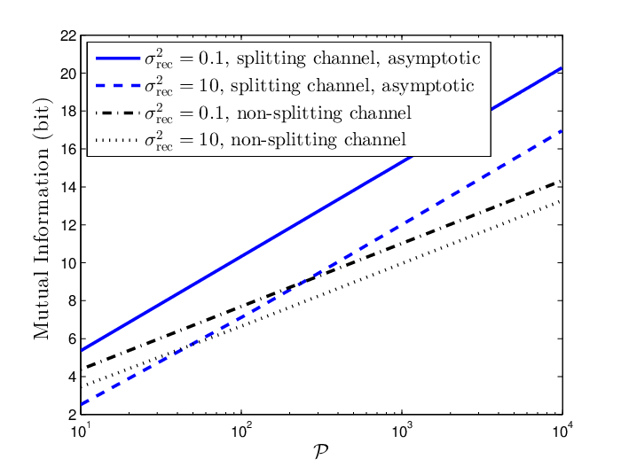
In the last two subsections, we have shown and explained that the splitting receiver achieves a $3/2$ fold rate gain compared with the non-splitting channels in the high SNR regime. This suggests that a notable performance improvement can be found within a moderate SNR range, which is verified as follows. Also, we verify the tightness of the asymptotic analytical results presented in Sec. III.B.

We consider the transmitted signal constellation of a general $M$-ary modulation scheme is $\Omega_{\mathrm{gen}}$, which is a two-dimensional constellation placed on the I-Q plane. The $i$th symbol is denoted by the tuple $({x}_{i},{y}_{i})$ on the I-Q plane, $i=1,2,...,M$. Specifically:

1. (i)

   For the $M$-PAM scheme [1], which is a one-dimensional modulation scheme on the I-axis, we have ${x}_{i}=2i-1$ for $i=1,2,...,M/2$, and ${x}_{i}=-x_{i-M/2}$ for $i=M/2+1,...M$, and $y_{i}=0$ for all $i$.

2. (ii)

   For the $M$-QAM scheme, which is a two-dimensional modulation scheme on the I-Q plane, we have ${x}_{i}=2\left(i\mod{\frac{\sqrt{M}}{2}}\right)-1$, ${y}_{i}=2\left\lfloor\frac{i-1}{\sqrt{M}/2}\right\rfloor-1$, $i=1,2,...,M/4$, which are the first quadrant symbols on the I-Q plane. Due to the symmetry property of $M$-QAM, the other quadrant symbol expressions are omitted for brevity.

3. (iii)

   For the $M$-IM scheme, which is a one-dimensional modulation scheme on the positive I-axis where the information is carried by the signal power but not phase, we have $x_{i}=\sqrt{2(i-1)}$ and $y_{i}=0$, $i=1,2,...,M$.

Based on the received signal expression after MRC in (5), the average signal power of the coherently and non-coherently processed signals are $\Theta_{1}\mathcal{P}$ and $\sqrt{\Theta_{2}}\mathcal{P}$, respectively. Thus, with such average power constraints, we define the noiseless received signal constellation $\breve{\Omega}_{\mathrm{gen}}$, and the $i$th symbol in $\breve{\Omega}_{\mathrm{gen}}$ is denoted by the tuple $(\breve{x}_{i},\breve{y}_{i},\breve{z}_{i})$, and $\breve{x}_{i}=k_{1}\sqrt{\Theta_{1}\mathcal{P}}{x}_{i}$, $\breve{y}_{i}=k_{1}\sqrt{\Theta_{1}\mathcal{P}}{y}_{i}$, $\breve{z}_{i}=k_{2}\sqrt{\Theta_{2}}\mathcal{P}\left(x^{2}_{i}+y^{2}_{i}\right)$. Here $k_{1}$ and $k_{2}\triangleq k^{2}_{1}$ are the power normalization parameters determined only by the geometric property of a certain modulation scheme. Specifically, we have

$$k_{1}=\left\{\begin{aligned} &\sqrt{\frac{3}{M^{2}-1}},&M\text{-PAM},\\ &\sqrt{\frac{3}{2(M-1)}},&M\text{-QAM},\\ &\sqrt{\frac{1}{M-1}},&M\text{-IM}.\end{aligned}\right.$$

(25)

For the single-antenna scenario, Figs. 11(a) and 11(c) show that the splitting ratio ${\rho}\in(0,1)$ bends the received signal constellation from the I-axis to a paraboloid in the I-P plane, for $4$-PAM and $4$-IM, respectively. Fig. 11(b) shows that the splitting ratio ${\rho}\in(0,1)$ bends the received signal constellation from the I-Q plane to a paraboloid in the I-Q-P space.

Since all the transmitted symbols are of equal probability, the optimal signal detection method is the maximum likelihood (ML) method [1]. The decision region for the $i$th symbol is defined as

$$\mathcal{V}_{i}\triangleq\left\{{\bm{v}}|f({\bm{v}}|i)\geq f({\bm{v}}|j),\forall j\neq i,{\bm{v}}\in\mathbb{R}^{3}\right\},$$

(26)

where ${\bm{v}}\triangleq(x,y,z)$ is the three-dimensional post-processing (noise added) signal in the splitting receiver, and $f(\cdot|\cdot)$ is the conditional pdf.

From Sec. III, since both the CD and PD circuits introduce additive Gaussian noise, the received signal is surrounded by the noise sphere (ellipsoid) in the I-Q-P space, and $f({\bm{v}}|i)$ is thus given by

$$f({\bm{v}}|i)=\frac{1}{\sigma^{2}_{\mathrm{cov}}\pi\sqrt{2\sigma^{2}_{\mathrm{rec}}\pi}}\exp\left(-\frac{(x-x_{i})^{2}}{\sigma^{2}_{\mathrm{cov}}}-\frac{(y-y_{i})^{2}}{\sigma^{2}_{\mathrm{cov}}}-\frac{(z-z_{i})^{2}}{2\sigma^{2}_{\mathrm{rec}}}\right).$$

(27)

Therefore, (26) is rewritten as

$$\mathcal{V}_{i}\triangleq\left\{(x,y,z):\ d_{i}(x,y,z)\leq d_{j}(x,y,z),\forall j\neq i\right\},$$

(28)

where

$$d_{j}(x,y,z)\triangleq\frac{\left(x-x_{j}\right)^{2}}{\sigma^{2}_{\mathrm{cov}}/2}+\frac{\left(y-y_{j}\right)^{2}}{\sigma^{2}_{\mathrm{cov}}/2}+\frac{\left(z-z_{j}\right)^{2}}{\sigma^{2}_{\mathrm{rec}}}.$$

(29)

From (28) and (29), after simplification, the decision region of the $i$th symbol, $\mathcal{V}_{i}$ is given by

$$\mathcal{V}_{i}=\left\{(x,y,z):\ \frac{\breve{x}_{j}-\breve{x}_{i}}{\sigma^{2}_{\mathrm{cov}}}\ x+\frac{\breve{y}_{j}-\breve{y}_{i}}{\sigma^{2}_{\mathrm{cov}}}\ y+\frac{\breve{z}_{j}-\breve{z}_{i}}{2\sigma^{2}_{\mathrm{rec}}}\ z\leq\frac{\breve{x}^{2}_{j}+\breve{y}^{2}_{j}-\breve{x}^{2}_{i}-\breve{y}^{2}_{i}}{2\sigma^{2}_{\mathrm{cov}}}+\frac{\breve{z}^{2}_{j}-\breve{z}^{2}_{i}}{4\sigma^{2}_{\mathrm{rec}}},\forall j\neq i\right\},$$

(30)

where $\breve{x}_{i}$, $\breve{y}_{i}$ and $\breve{z}_{i}$ are defined in Sec. IV.B above (25). It is easy to see that $\mathcal{V}_{i}$ is bounded by planes. The plane implied in (30), which divides the decision region between the $i$th and $j$th receive symbols, is given by

$$\mathcal{A}_{i-j}\triangleq\left\{(x,y,z):\ \frac{\breve{x}_{j}-\breve{x}_{i}}{\sigma^{2}_{\mathrm{cov}}}\ x+\frac{\breve{y}_{j}-\breve{y}_{i}}{\sigma^{2}_{\mathrm{cov}}}\ y+\frac{\breve{z}_{j}-\breve{z}_{i}}{2\sigma^{2}_{\mathrm{rec}}}\ z=\frac{\breve{x}^{2}_{j}+\breve{y}^{2}_{j}-\breve{x}^{2}_{i}-\breve{y}^{2}_{i}}{2\sigma^{2}_{\mathrm{cov}}}+\frac{\breve{z}^{2}_{j}-\breve{z}^{2}_{i}}{4\sigma^{2}_{\mathrm{rec}}}\right\}.$$

(31)

References

- [1] D. Tse and P. Viswanath, Fundamentals of wireless communication. Cambridge university press, 2005.
- [2] A. Alkhateeb, J. Mo, N. Gonzalez-Prelcic, and R. W. Heath, “MIMO precoding and combining solutions for millimeter-wave systems,” IEEE Commun. Mag., vol. 52, no. 12, pp. 122–131, Dec. 2014.
- [3] J. G. Andrews, T. Bai, M. Kulkarni, A. Alkhateeb, A. Gupta, and R. W. Heath, Jr, “Modeling and Analyzing Millimeter Wave Cellular Systems,” ArXiv e-prints. [Online]. Available: https://arxiv.org/pdf/1605.04283v1.pdf
- [4] M. Chowdhury, A. Manolakos, and A. Goldsmith, “Scaling laws for noncoherent energy-based communications in the SIMO MAC,” IEEE Trans. Inf. Theory, vol. 62, no. 4, pp. 1980–1992, Apr. 2016.
- [5] L. Jing, E. D. Carvalho, P. Popovski, and . O. Martínez, “Design and performance analysis of noncoherent detection systems with massive receiver arrays,” IEEE Trans. Signal Process., vol. 64, no. 19, pp. 5000–5010, Oct. 2016.
- [6] S. Bi, C. Ho, and R. Zhang, “Wireless powered communication: Opportunities and challenges,” IEEE Commun. Mag., vol. 53, no. 4, pp. 117–125, Apr. 2015.
- [7] K. Huang and X. Zhou, “Cutting the last wires for mobile communications by microwave power transfer,” IEEE Commun. Mag., vol. 53, no. 6, pp. 86–93, Jun. 2015.
- [8] I. Krikidis, S. Timotheou, S. Nikolaou, G. Zheng, D. Ng, and R. Schober, “Simultaneous wireless information and power transfer in modern communication systems,” IEEE Commun. Mag., vol. 52, no. 11, pp. 104–110, Nov. 2014.
- [9] X. Lu, P. Wang, D. Niyato, D. I. Kim, and Z. Han, “Wireless networks with RF energy harvesting: A contemporary survey,” IEEE Commun. Surveys Tuts., vol. 17, no. 2, pp. 757–789, Second quarter 2015.
- [10] J. M. Kahn and J. R. Barry, “Wireless infrared communications,” Proc. IEEE, vol. 85, no. 2, pp. 265–298, Feb. 1997.
- [11] K. Szczerba, P. Westbergh, J. Karout, J. S. Gustavsson, Å. Haglund, M. Karlsson, P. A. Andrekson, E. Agrell, and A. Larsson, “4-PAM for high-speed short-range optical communications,” IEEE J. Opt. Commun. Netw., vol. 4, no. 11, pp. 885–894, Nov. 2012.
- [12] A. Lapidoth, S. Moser, and M. Wigger, “On the capacity of free-space optical intensity channels,” IEEE Trans. Inf. Theory, vol. 55, no. 10, pp. 4449–4461, Oct. 2009.
- [13] Y. Wu, Y. Liu, Q. Xue, S. Li, and C. Yu, “Analytical design method of multiway dual-band planar power dividers with arbitrary power division,” IEEE Trans. Microw. Theory Tech., vol. 58, no. 12, pp. 3832–3841, Dec. 2010.
- [14] DC to 18 GHz Power Splitter, Agilent Technologies. [Online]. Available: http://cp.literature.agilent.com/litweb/pdf/5990-5351EN.pdf
- [15] X. Zhou, R. Zhang, and C. K. Ho, “Wireless information and power transfer: Architecture design and rate-energy tradeoff,” IEEE Trans. Commun., vol. 61, no. 11, pp. 4754–4767, Nov. 2013.
- [16] W. Liu, X. Zhou, S. Durrani, and P. Popovski, “SWIPT with practical modulation and RF energy harvesting sensitivity,” in Proc. IEEE ICC, May 2016, pp. 1–7.
- [17] T. Cover and J. Thomas, Elements of Information Theory. Wiley, 2006.
- [18] E. Grushka, “Characterization of exponentially modified Gaussian peaks in chromatography,” Analytical Chemistry, vol. 44, no. 11, pp. 1733–1738, 1972.
- [19] A. Kraskov, H. Stögbauer, and P. Grassberger, “Estimating mutual information,” Physical review E, vol. 69, no. 6, p. 066138, 2004.
- [20] M. Abramowitz and I. A. Stegun, Handbook of mathematical functions: with formulas, graphs, and mathematical tables. Courier Corporation, 1964, vol. 55.