Learning to Reason: End-to-End Module Networks
for Visual Question Answering
Abstract
Natural language questions are inherently compositional, and many are most easily answered by reasoning about their decomposition into modular sub-problems. For example, to answer “is there an equal number of balls and boxes?” we can look for balls, look for boxes, count them, and compare the results. The recently proposed Neural Module Network (NMN) architecture [3, 2] implements this approach to question answering by parsing questions into linguistic substructures and assembling question-specific deep networks from smaller modules that each solve one subtask. However, existing NMN implementations rely on brittle off-the-shelf parsers, and are restricted to the module configurations proposed by these parsers rather than learning them from data. In this paper, we propose End-to-End Module Networks (N2NMNs), which learn to reason by directly predicting instance-specific network layouts without the aid of a parser. Our model learns to generate network structures (by imitating expert demonstrations) while simultaneously learning network parameters (using the downstream task loss). Experimental results on the new clevr dataset targeted at compositional question answering show that N2NMNs achieve an error reduction of nearly 50% relative to state-of-the-art attentional approaches, while discovering interpretable network architectures specialized for each question.
1 Introduction

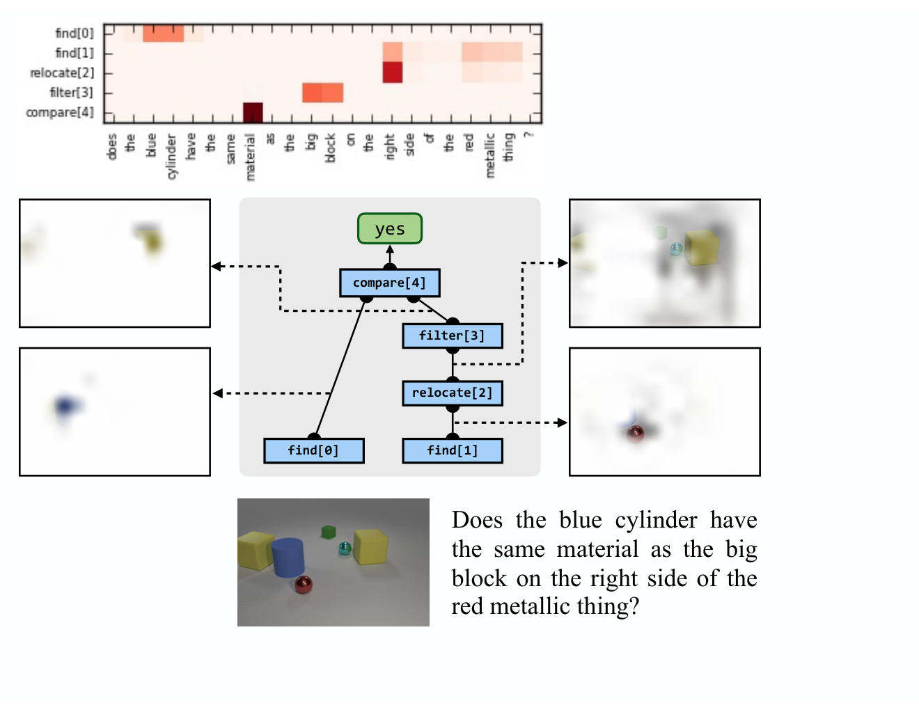
Visual Question Answering (VQA) requires joint comprehension of images and text. This comprehension often depends on compositional reasoning, for example locating multiple objects in a scene and inspecting their properties or comparing them to one another (Figure 1). While conventional deep networks have shown promising VQA performance [9], there is limited evidence that they are capable of explicit compositional reasoning [15]. Much of the success of state-of-the-art approaches to VQA instead comes from their ability to discover statistical biases in the data distribution [10]. And to the extent that such approaches are capable of more sophisticated reasoning, their monolithic structure makes these behaviors difficult to understand and explain. Additionally, they rely on the same non-modular network structure for all input questions.
In this paper, we propose End-to-End Module Networks (N2NMNs): a class of models capable of predicting novel modular network architectures directly from textual input and applying them to images in order to solve question answering tasks. In contrast to previous work, our approach learns to both parse the language into linguistic structures and compose them into appropriate layouts.
The present work synthesizes and extends two recent modular architectures for visual problem solving. Standard neural module networks (NMNs) [3] already provide a technique for constructing dynamic network structures from collections of composable modules. However, previous work relies on an external parser to process input text and obtain the module layout. This is a serious limitation, because off-the-shelf language parsers are not designed for language and vision tasks and must therefore be modified using handcrafted rules that often fail to predict valid layouts [15]. Meanwhile, the compositional modular network [12] proposed for grounding referring expressions in images does not need a parser, but is restricted to a fixed (subject, relationship, object) structure. None of the existing methods can learn to predict a suitable structure for every input in an end-to-end manner.
Our contributions are 1) a method for learning a layout policy that dynamically predicts a network structure for each instance, without the aid of external linguistic resources at test time and 2) a new module parameterization that uses a soft attention over question words rather than hard-coded word assignments. Experiments show that our model is capable of directly predicting expert-provided network layouts with near-perfect accuracy, and even improving on expert-designed networks after a period of exploration. We obtain state-of-the-art results on the recently released clevr dataset by a wide margin.
2 Related work

Neural module networks. The recently proposed neural module network (NMN) architecture [3]—a general class of recursive neural networks [22]—provides a framework for constructing deep networks with dynamic computational structure. In an NMN model, every input is associated with a layout that provides a template for assembling an instance-specific network from a collection of shallow network fragments called modules. These modules can be jointly trained across multiple structures to provide reusable, compositional behaviors. Existing work on NMNs has focused on natural language question answering applications, in which a linguistic analysis of the question is used to generate the layout, and the resulting network applied to some world representation (either an image or knowledge base) to produce an answer. The earliest work on NMNs [3] used fixed rule-based layouts generated from dependency parses [27]. Later work on “dynamic” module networks (D-NMNs) [2] incorporated a limited form of layout prediction by learning to rerank a list of three to ten candidates, again generated by rearranging modules predicted by a dependency parse. Like D-NMNs, the present work attempts to learn an optimal layout predictor jointly with module behaviors themselves. Here, however, we tackle a considerably more challenging prediction problem: our approach learns to optimize over the full space of network layouts rather than acting as a reranker, and requires no parser at evaluation time.
We additionally modify the representation of the assembled module networks themselves: where [3] and [2] parameterized individual modules with a fixed embedding supplied by the parser, here we predict these parameters jointly with network structures using a soft attention mechanism. This parameterization resembles the approach used in the “compositional modular network” architecture [12] for grounding referential expressions. However, the model proposed in [12] is restricted to a fixed layout structure of (subject, relationship, object) for every referential expression, and includes no structure search.
Learning network architectures. More generally than these dynamic / modular approaches, a long line of research focuses on generic methods for automatically discovering neural network architectures from data. Past work includes techniques for optimizing over the space of architectures using evolutionary algorithms [23, 8], Bayesian methods [6], and reinforcement learning [28]. The last of these is most closely related to our approach in this paper: both learn a controller RNN to output a network structure, train a neural network with the generated structure, and use the accuracy of the generated network to optimize the controller RNN. A key difference between [28] and the layout policy optimization in our work is that [28] learns a fixed layout (network architecture) that is applied to every instance, while our model learns a layout policy that dynamically predicts a specific layout tailored to each individual input example.
Visual question answering. The visual question answering task [19] is generally motivated as a test to measure the capacity of deep models to reason about linguistic and visual inputs jointly [19]. Recent years have seen a proliferation of datasets [19, 4] and approaches, including models based on differentiable memory [25, 24], dynamic prediction of question-specific computations [20, 2], and core improvements to the implementation of the multi-modal representation and attention mechanism [9, 18]. Together, these approaches have produced substantial gains over the initial baseline results published with the first VQA datasets.
It has been less clear, however, that these improvements correspond to an improvement in the reasoning abilities of models. Recent work has found that it is possible to do quite well on many visual QA problems by simply memorizing statistics about question / answer pairs [10] (suggesting that limited visual reasoning is involved), and that models with bag-of-words text representations perform competitively against more sophisticated approaches [14] (suggesting that limited linguistic compositionality is involved). To address this concern, newer visual question answering datasets have focused on exploring specific phenomena in compositionality and generalization; examples include the shapes dataset [3], the VQAv2 dataset [10], and the clevr dataset [15]. The last of these appears to present the greatest challenges to standard VQA approaches and the hardest reasoning problems in general.
Most previous work on this task other than NMN uses a fixed inference structure to answer every question. However, the optimal reasoning procedure may vary greatly from question to question, so it is desirable to have inference structures that are specific to the input question. Concurrent with our work, [16] proposes a similar model to ours. Our model is different from [16] in that we use a set of specialized modules with soft attention mechanism to provide textual parameters for each module, while [16] uses a generic module implementation with textual parameters hard-coded in module instantiation.
3 End-to-End Module Networks
We propose End-to-End Module Networks (N2NMNs) to address compositionality in visual reasoning tasks. Our model consists of two main components: a set of co-attentive neural modules that provide parameterized functions for solving sub-tasks, and a layout policy to predict a question-specific layout from which a neural network is dynamically assembled. An overview of our model is shown in Figure 2.
Given an input question, such as how many other things are there of the same size as the matte ball?, our layout policy first predicts a coarse functional expression like count(relocate(find()) that describes the structure of the desired computation, Next, some subset of function applications within this expression (here relocate and find) receive parameter vectors predicted from text (here perhaps vector representations of matte ball and size, respectively). Then a network is assembled with the modules according to this layout expression to output an answer.
We describe the implementation details of each neural module in Sec. 3.1, and our layout policy in Sec. 3.2. In Sec. 3.3, we present a reinforcement learning approach to jointly optimize the neural modules and the layout policy.
3.1 Attentional neural modules
| Module name | Att-inputs | Features | Output | Implementation details |
|---|---|---|---|---|
| find | (none) | , | att | |
| relocate | , | att | ||
| and | (none) | att | ||
| or | (none) | att | ||
| filter | , | att | , i.e. reusing find and and | |
| [exist, count] | (none) | ans | ||
| describe | , | ans | ||
| [eq_count, more, less] | (none) | ans | ||
| compare | , | ans |
Our model involves a set of neural modules that can be dynamically assembled into a neural network. A neural module is a parameterized function that takes zero, one or multiple tensors as input, using its internal parameter and features and from the image and question to perform some computation on the input, and outputs a tensor . In our implementation, each input tensor is an image attention map over the convolutional image feature grid, and the output tensor is either an image attention map, or a probability distribution over possible answers.
Table 1 shows the set of modules in our N2NMNs model, along with their implementation details. We assign a name to each module according to its input and output type and potential functionality, such as find or describe. However, we note that each module is in itself merely a function with parameters, and we do not restrict its behavior during training. In addition to the input tensors (that are outputs from other modules), a module can also use two additional feature vectors and , where is the spatial feature map extracted from the image with a convolutional neural network, and is a textual vector for this module that contains information extracted from the question . In addition, and and or take two image attention maps as inputs, and return their intersection or union respectively.
In Table 1, the find module outputs an attention map over the image and can be potentially used to localize some objects or attributes. The relocate module transforms the input image attention map and outputs a new attention map, which can be useful for spatial or relationship inference. Also the filter module reuses find and and, and can be used to simplify the layout expression. We use two classes of modules to infer an answer from a single attention map: the first class has the instances exist and count (instances share the same structure, but have different parameters). They are used for simple inference by looking only at the attention map. The second class, describe, is for more complex inference where visual appearance is needed. Similarly, for pairwise comparison over two attention maps we also have two classes of available modules with (compare) or without (eq_count,more,less) access to visual features.
The biggest difference in module implementation between this work and [3] is the textual component. Hard-coded textual components are used in [3], for example, describe[‘shape’] and describe[‘where’] are two different instantiations that have different parameters. In contrast, our model obtains the textual input using soft attention over question words similar to [12]. For each module , we predict an attention map over the question words (in Sec. 3.2), and obtain the textual feature for each module:
| (1) |
where is the word embedding vector for word in the question. At runtime, the modules can be assembled into a network according to a layout , which is a computation expression consisting of modules, such as , where each of is one of the modules in Table 1.
3.2 Layout policy with sequence-to-sequence RNN
We would like to predict the most suitable reasoning structure tailored to each question. For an input question such as What object is next to the table?, our layout policy outputs a probability distribution , and we can sample from to obtain high probability layout such as describe(relocate(find())) that are effective for answering the question . Then, a neural network is assembled according to the predicted layout to output an answer.
Unlike in [2] where the layout search space is restricted to a few parser candidates, in this work, we search over a much larger layout space: in our model, the layout policy predicts a distribution over the space of all possible layouts. Every possible layout is an expression that consists of neural modules, such as , and can be represented as a syntax tree. So each layout expression can be mapped one-to-one into a linearized sequence using Reverse Polish Notation [7] (the post-order traversal over the syntax tree). Figure 3 shows an example for an expression and its linearized module token sequence.
After linearizing each layout into a sequence of module tokens , the layout prediction problem turns into a sequence-to-sequence learning problem from questions to module tokens. We address this problem using the attentional Recurrent Neural Network [5]. First, we embed every word in the question into a vector (also embedding all module tokens similarly), and use a multi-layer LSTM network as the encoder of the input question. For a question with words, the encoder LSTM outputs a length- sequence . The decoder is a LSTM network that has the same structure as the encoder but different parameters. Similar to [5], at each time step in the decoder LSTM, a soft attention map over the input sequence is predicted. At decoder time-step , the attention weights of input word at position are predicted as
| (2) | |||||
| (3) |
where and are LSTM outputs at encoder time-step and decoder time-step , respectively, and , and are model parameters to be learned from data. Then a context vector is obtained as , and the probability for the next module token is predicted from and as . We sample from to discretely get the next token , and also construct its textual input according to Eqn. 1 using the attention weights in Eqn. 3. The probability of a layout is . At test time, we deterministically predict a maximum-probability layout from using beam search, and assemble a neural network according to to output an answer for the question.
3.3 End-to-end training
During training, we jointly learn the layout policy and the parameters in each neural module, and minimize the expected loss from the layout policy. Let be all the parameters in our model. Suppose we obtain a layout sampled from and receive a final question answering loss on question and image after predicting an answer using the network assembled with . Our training loss function is as follows.
| (4) |
where we use the softmax loss over the output answer scores as in our implementation.
The loss function in is not fully differentiable since the layout is discrete, so one cannot train it with full back-propagation. We optimize using back-propagation for differentiable parts, and policy gradient method in reinforcement learning for non-differentiable part. The gradient of the loss is which can be estimated using Monte-Carlo sampling as
| (5) |
where both and are fully differentiable so the above equation can be computed with back-propagation, allowing end-to-end training for the entire model. We use in our implementation.
To reduce the variance of the estimated gradient, we introduce a simple baseline , by replacing with in Eqn. 5, where is implemented as an exponential moving average over the recent loss . We also use an entropy regularization over the policy to encourage exploration through the layout space.
Behavioral cloning from expert polices.
Optimizing the loss function in Eqn. 4 from scratch is a challenging reinforcement learning problem: one needs to simultaneously learn the parameters in the sequence-to-sequence RNN to optimize the layout policy and textual attention weights to construct the textual features for each module, and also the parameters in the neural modules. This is more challenging than a typical reinforcement learning scenario where one only needs to learn a policy.
On the other hand, the learning would be easier if we have some additional knowledge of module layout. While we do not want to restrict the layout search space to only a few candidates from the parser as in [2], we can treat these candidate layouts as an existing expert policy that can be used to provide additional supervision. More generally, if there is an expert policy that predicts a reasonable layout from the question, we can first pre-train our model by behavioral cloning from . This can be done by minimizing the KL-divergence between the expert policy and our layout policy , and simultaneously minimizing the question answering loss with obtained from . This supervised behavioral cloning from the expert policy can provide a good set of initial parameters in our sequence-to-sequence RNN and each neural module. Note that the above behavioral cloning procedure is only done at training time to obtain a supervised initialization our model, and the expert policy is not used at test time.
The expert policy is not necessarily optimal, so behavioral cloning itself is not sufficient for learning the most suitable layout for each question. After learning a good initialization by cloning the expert policy, our model is further trained end-to-end with gradient computed using Eqn. 5, where now the layout is sampled from the layout policy in our model, and the expert policy can be discarded.
We train our models using the Adam Optimizer [17] in all of our experiments. Our model is implemented using TensorFlow [1] and our code is available at http://ronghanghu.com/n2nmn/.
4 Experiments
We first analyze our model on a relatively small shapes dataset [3], and then apply our model to two large-scale datasets: clevr [15] and vqa [4].
4.1 Analysis on the shapes dataset
The shapes dataset for visual question answering (collected in [3]) consists of 15616 image-question pairs with 244 unique questions. Each image consists of shapes of different colors and sizes aligned on a 3 by 3 grid. Despite its relatively small size, effective reasoning is needed to successfully answer questions like “is there a red triangle above a blue shape?”. The dataset also provides a ground-truth parsing result for each question, which is used to train the NMN model in [3].
We analyze our method on the shapes dataset under two settings. In the first setting, we train our model using behavioral cloning from an expert layout policy as described in Sec. 3.3. An expert layout policy is constructed by mapping the the ground-truth parsing for each question to a module layout in the same way as in [3]. Note that unlike [3], in this setting we only need to query the expert policy at training time. At test time, we obtain the layout from the learned layout policy in our model, while NMN [3] still needs to access the ground-truth parsing at test time.
In the second setting, we train our model without using any expert policy, and directly perform policy optimization by minimizing the loss function in Eqn. 4 with gradient in Eqn. 5. For both settings, we use a simple randomly initialized two-layer convolutional neural network to extract visual features from the image, trained together with other parts of our model.
| Method | Accuracy |
|---|---|
| NMN [3] | 90.80% |
| ours - behavioral cloning from expert | 100.00% |
| ours - policy search from scratch | 96.19% |

The results are summarized in Table 2. In the first setting, we find that our model (“ours - behavioral cloning from expert”) already achieves accuracy. While this shows that the expert policy constructed from ground-truth parsing is quite effective on this dataset, the higher performance of our model compared to the previous NMN [3] also suggests that our implementation of modules is more effective than [3], since the NMN is also trained with the same expert module layout obtained from the ground-truth parsing. In the second setting, our model achieves a good performance on this dataset by performing policy search from scratch without resorting to any expert policy. Figure 4 shows some examples of predicted layouts and answers on this dataset.

4.2 Evaluation on the clevr dataset
| Compare Integer | Query Attribute | Compare Attribute | ||||||||||||
| Method | Overall | Exist | Count | equal | less | more | size | color | material | shape | size | color | material | shape |
| CNN+BoW [26] | 48.4 | 59.5 | 38.9 | 50 | 54 | 49 | 56 | 32 | 58 | 47 | 52 | 52 | 51 | 52 |
| CNN+LSTM [4] | 52.3 | 65.2 | 43.7 | 57 | 72 | 69 | 59 | 32 | 58 | 48 | 54 | 54 | 51 | 53 |
| CNN+LSTM+MCB [9] | 51.4 | 63.4 | 42.1 | 57 | 71 | 68 | 59 | 32 | 57 | 48 | 51 | 52 | 50 | 51 |
| CNN+LSTM+SA [25] | 68.5 | 71.1 | 52.2 | 60 | 82 | 74 | 87 | 81 | 88 | 85 | 52 | 55 | 51 | 51 |
| NMN (expert layout) [3] | 72.1 | 79.3 | 52.5 | 61.2 | 77.9 | 75.2 | 84.2 | 68.9 | 82.6 | 80.2 | 80.7 | 74.4 | 77.6 | 79.3 |
| ours - policy search from scratch | 69.0 | 72.7 | 55.1 | 71.6 | 85.1 | 79.0 | 88.1 | 74.0 | 86.6 | 84.1 | 50.1 | 53.9 | 48.6 | 51.1 |
| ours - cloning expert | 78.9 | 83.3 | 63.3 | 68.2 | 87.2 | 85.4 | 90.5 | 80.2 | 88.9 | 88.3 | 89.4 | 52.5 | 85.4 | 86.7 |
| ours - policy search after cloning | 83.7 | 85.7 | 68.5 | 73.8 | 89.7 | 87.7 | 93.1 | 84.8 | 91.5 | 90.6 | 92.6 | 82.8 | 89.6 | 90.0 |
question: do the small cylinder that is in front of the small green thing and the object right of the green cylinder have the same material?
ground-truth answer: no
image
layout
find[0]
relocate[1]
filter[2]
find[3]
relocate[4]
compare[5]


 image
layout
find[0]
relocate[1]
filter[2]
find[3]
relocate[4]
filter[5]
compare[6]
image
layout
find[0]
relocate[1]
filter[2]
find[3]
relocate[4]
filter[5]
compare[6]


We evaluate our End-to-End Module Networks on the recently proposed clevr dataset [15] with 100,000 images and 853,554 questions. The images in this dataset are photo-realistic rendered images with objects of different shapes, colors, materials and sizes and possible occlusions, and the questions in this dataset are synthesized with functional programs. Compared to other datasets for visual question answering such as [4], the clevr dataset focuses mostly on the reasoning ability. The questions in the clevr dataset have much longer question length, and require handling long and complex inference chains to get an answer, such as “what size is the cylinder that is left of the brown metal thing that is left of the big sphere?” and “there is an object in front of the blue thing; does it have the same shape as the tiny cyan thing that is to the right of the gray metal ball?”.
In our experiment on this dataset, we resize each image to , and extract a convolutional feature map from each image by forwarding the image through the VGG-16 network [21] trained on ImageNET classification, and take the 512-channel pool5 output. To help reason about spatial properties, we add two extra and dimensions to each location on the feature map similar to [13], so the final visual feature on each image is a tensor. Each question word is embedded to a 300-dimensional vector initialized from scratch. We use a batch size of 64 during training.
In the first training stage, behavioral cloning is used with an expert layout policy as described in Sec. 3.3. We construct an expert layout policy that deterministically maps a question into a layout by converting the annotated functional programs in this dataset into a module layout with manually defined rules: first, the program chain is simplified to keep all intermediate computation in the image attention domain, and then each function type is mapped to a module in Table 1 that has the same number of inputs and closest potential behavior.
While the manually specified expert policy obtained in this way might not be optimal, it is sufficient to provide supervision to learn good initial model parameters that can be further optimized in the later stage. During behavioral cloning, we train our model with two losses added together: the first loss is the KL-divergence , which corresponds to maximizing the probability of the expert layout in our policy from the sequence-to-sequence RNN, and the second loss is the question answering loss for question and image , where the layout is obtained from the expert. Note that the second loss also affects the parameters in the sequence-to-sequence RNN through the textual attention in Eqn. 3.
After the first training stage, we discard the expert policy and continue to train our model for a second stage with end-to-end reinforcement learning, using the gradient in Eqn. 5. In this stage, the model is no longer constrained to get close to the expert, but is encouraged to explore the layout space and search for the optimal layout of each question.
As a baseline, we also train our model without using any expert policy, and directly perform policy search from scratch by minimizing the loss function in Eqn. 4.
We evaluate our model on the test set of clevr. Table 3 shows the detailed performance of our model and previous methods on each question type, where “ours - policy search from scratch” is the baseline using pure reinforcement learning without resorting to the expert, “ours - cloning expert” is the supervised behavioral cloning from the constructed expert policy in the first stage, and “ours - policy search after cloning” is our model further trained for the second training stage. It can be seen that without using any expert demonstrations, our method with policy optimization from scratch already achieves higher performance than most previous work, and our model trained in the first behavioral cloning stage outperforms the previous approaches by a large margin in overall accuracy. This indicates that our neural modules are capable of reasoning for complex questions in the dataset like “does the block that is to the right of the big cyan sphere have the same material as the large blue thing?” Our model also outperforms the NMN baseline [3] trained on the same expert layout as used in our model11 1 The question parsing in the original NMN implementation does not work on the clevr dataset, as confirmed in [15]. For fair comparison with NMN, we train NMN using the same expert layout as our model.. This shows that our soft attention module parameterization is better than the hard-coded textual parameters in NMN. Figure 5 shows some question answering examples with our model.
By comparing “ours - policy search after cloning” with “ours - cloning expert” in Table 3, it can be seen that the performance consistently improves after end-to-end training with policy search using reinforcement learning in the second training stage, with especially large improvement on the compare color type of questions, indicating that the original expert policy is not optimal, and we can improve upon it with policy search over the entire layout space. Figure 6 shows an example before and after end-to-end optimization.
5 Evaluation on the vqa dataset

We also evaluate our method on the vqa dataset [4] with real images. On the vqa dataset, although there are no underlying functional program annotation for the questions, we can still construct an expert layout policy using a syntactic parse of questions as in [3, 2], and train our model in the same way as in Sec. 4.2. We train our model using different visual features for fair comparison with other methods. Unlike previous work [3, 2], the syntactic parser is only used during the training stage and is not needed at test time.
| Method | Visual feature | Accuracy |
|---|---|---|
| NMN [3] | LRCN VGG-16 | 57.3 |
| D-NMN [2] | LRCN VGG-16 | 57.9 |
| MCB [9] | ResNet-152 | 64.7 |
| ours - cloning expert | LRCN VGG-16 | 61.9 |
| ours - cloning expert | ResNet-152 | 64.2 |
| ours - policy search after cloning | ResNet-152 | 64.9 |
The results are summarized in Table 4 on the vqa dataset, where our method significantly outperforms NMN [3] and D-NMN [2] that also use modular structures, using the same LRCN VGG-16 image features (VGG-16 network fine-tuned for image captioning, as used in [3, 2]). Compared with MCB [9] (the VQA 2016 challenge winner method) trained on the same ResNet-152 image features, our model achieves slightly higher performance while being more interpretable as one can explicitly see the underlying reasoning procedure. Figure 7 shows a prediction example on this dataset.
6 Conclusion
In this paper, we present the End-to-End Module Networks for visual question answering. Our model uses a set of neural modules to break down complex reasoning problems posed in textual questions into a few sub-tasks connected together, and learns to predict a suitable layout expression for each question using a layout policy implemented with a sequence-to-sequence RNN. During training, the model can be first trained with behavioral cloning from an expert layout policy, and further optimized end-to-end using reinforcement learning. Experimental results demonstrate that our model is capable of handling complicated reasoning problems, and the end-to-end optimization of the neural modules and layout policy can lead to significant further improvement over behavioral cloning from expert layouts.
Acknowledgements. This work was supported by DARPA, AFRL, DoD MURI award N000141110688, NSF awards IIS-1427425, IIS-1212798 and IIS-1212928, NGA and the Berkeley Artificial Intelligence Research (BAIR) Lab. Jacob Andreas is supported by a Facebook graduate fellowship and a Huawei / Berkeley AI fellowship.
References
- [1] M. Abadi, A. Agarwal, P. Barham, E. Brevdo, Z. Chen, C. Citro, G. S. Corrado, A. Davis, J. Dean, M. Devin, S. Ghemawat, I. Goodfellow, A. Harp, G. Irving, M. Isard, Y. Jia, R. Jozefowicz, L. Kaiser, M. Kudlur, J. Levenberg, D. Mané, R. Monga, S. Moore, D. Murray, C. Olah, M. Schuster, J. Shlens, B. Steiner, I. Sutskever, K. Talwar, P. Tucker, V. Vanhoucke, V. Vasudevan, F. Viégas, O. Vinyals, P. Warden, M. Wattenberg, M. Wicke, Y. Yu, and X. Zheng. TensorFlow: Large-scale machine learning on heterogeneous systems. arXiv:1603.04467, 2016.
- [2] J. Andreas, M. Rohrbach, T. Darrell, and D. Klein. Learning to compose neural networks for question answering. In Proceedings of the Conference of the North American Chapter of the Association for Computational Linguistics (NAACL), 2016.
- [3] J. Andreas, M. Rohrbach, T. Darrell, and D. Klein. Neural module networks. In Proceedings of the IEEE Conference on Computer Vision and Pattern Recognition (CVPR), 2016.
- [4] S. Antol, A. Agrawal, J. Lu, M. Mitchell, D. Batra, C. L. Zitnick, and D. Parikh. Vqa: Visual question answering. In Proceedings of the IEEE International Conference on Computer Vision (ICCV), 2015.
- [5] D. Bahdanau, K. Cho, and Y. Bengio. Neural machine translation by jointly learning to align and translate. In Proceedings of the International Conference on Learning Representations (ICLR), 2015.
- [6] J. Bergstra, D. Yamins, and D. D. Cox. Making a science of model search: Hyperparameter optimization in hundreds of dimensions for vision architectures. ICML (1), 28:115–123, 2013.
- [7] A. W. Burks, D. W. Warren, and J. B. Wright. An analysis of a logical machine using parenthesis-free notation. Mathematical tables and other aids to computation, 8(46):53–57, 1954.
- [8] D. Floreano, P. Dürr, and C. Mattiussi. Neuroevolution: from architectures to learning. Evolutionary Intelligence, 1(1):47–62, 2008.
- [9] A. Fukui, D. H. Park, D. Yang, A. Rohrbach, T. Darrell, and M. Rohrbach. Multimodal compact bilinear pooling for visual question answering and visual grounding. In Proceedings of the Conference on Empirical Methods in Natural Language Processing (EMNLP), 2016.
- [10] Y. Goyal, T. Khot, D. Summers-Stay, D. Batra, and D. Parikh. Making the V in VQA matter: Elevating the role of image understanding in Visual Question Answering. CoRR, abs/1612.00837, 2016.
- [11] K. He, X. Zhang, S. Ren, and J. Sun. Deep residual learning for image recognition. In Proceedings of the IEEE Conference on Computer Vision and Pattern Recognition (CVPR), 2016.
- [12] R. Hu, M. Rohrbach, J. Andreas, T. Darrell, and K. Saenko. Modeling relationships in referential expressions with compositional modular networks. In Proceedings of the IEEE Conference on Computer Vision and Pattern Recognition (CVPR), 2017.
- [13] R. Hu, M. Rohrbach, and T. Darrell. Segmentation from natural language expressions. In Proceedings of the European Conference on Computer Vision (ECCV), 2016.
- [14] A. Jabri, A. Joulin, and L. van der Maaten. Revisiting visual question answering baselines. In European Conference on Computer Vision, pages 727–739. Springer, 2016.
- [15] J. Johnson, B. Hariharan, L. van der Maaten, L. Fei-Fei, C. L. Zitnick, and R. Girshick. Clevr: A diagnostic dataset for compositional language and elementary visual reasoning. In Proceedings of the IEEE Conference on Computer Vision and Pattern Recognition (CVPR), 2017.
- [16] J. Johnson, B. Hariharan, L. van der Maaten, J. Hoffman, L. Fei-Fei, C. L. Zitnick, and R. Girshick. Inferring and executing programs for visual reasoning. In Proceedings of the IEEE International Conference on Computer Vision (ICCV), 2017.
- [17] D. Kingma and J. Ba. Adam: A method for stochastic optimization. In Proceedings of the International Conference on Learning Representations (ICLR), 2015.
- [18] J. Lu, J. Yang, D. Batra, and D. Parikh. Hierarchical Co-Attention for Visual Question Answering. In Advances in Neural Information Processing Systems (NIPS), 2016.
- [19] M. Malinowski and M. Fritz. A multi-world approach to question answering about real-world scenes based on uncertain input. In Advances in Neural Information Processing Systems (NIPS), 2014.
- [20] H. Noh, P. H. Seo, and B. Han. Image question answering using convolutional neural network with dynamic parameter prediction. In Proceedings of the IEEE Conference on Computer Vision and Pattern Recognition (CVPR), 2016.
- [21] K. Simonyan and A. Zisserman. Very deep convolutional networks for large-scale image recognition. In Proceedings of the International Conference on Learning Representations (ICLR), 2015.
- [22] R. Socher, A. Perelygin, J. Y. Wu, J. Chuang, C. D. Manning, A. Y. Ng, C. Potts, et al. Recursive deep models for semantic compositionality over a sentiment treebank. In Proceedings of the conference on empirical methods in natural language processing (EMNLP), volume 1631, page 1642. Citeseer, 2013.
- [23] D. Wierstra, F. J. Gomez, and J. Schmidhuber. Modeling systems with internal state using evolino. In Proceedings of the 7th annual conference on Genetic and evolutionary computation, pages 1795–1802. ACM, 2005.
- [24] C. Xiong, S. Merity, and R. Socher. Dynamic memory networks for visual and textual question answering. In Proceedings of the International Conference on Machine Learning (ICML), 2016.
- [25] Z. Yang, X. He, J. Gao, L. Deng, and A. Smola. Stacked attention networks for image question answering. In Proceedings of the IEEE Conference on Computer Vision and Pattern Recognition (CVPR), 2016.
- [26] B. Zhou, Y. Tian, S. Sukhbaatar, A. Szlam, and R. Fergus. Simple baseline for visual question answering. In Proceedings of the European Conference on Computer Vision (ECCV), 2016.
- [27] M. Zhu, Y. Zhang, W. Chen, M. Zhang, and J. Zhu. Fast and accurate shift-reduce constituent parsing. In ACL (1), pages 434–443, 2013.
- [28] B. Zoph and Q. V. Le. Neural architecture search with reinforcement learning. In Proceedings of the International Conference on Learning Representations (ICLR), 2017.