A geometric approach to non-linear correlations with intrinsic scatter
Abstract
We propose a new mathematical model for -dimensional non-linear correlations with intrinsic scatter in -dimensional data. The model is based on Riemannian geometry, and is naturally symmetric with respect to the measured variables and invariant under coordinate transformations. We combine the model with a Bayesian approach for estimating the parameters of the correlation relation and the intrinsic scatter. A side benefit of the approach is that censored and truncated datasets and independent, arbitrary measurement errors can be incorporated. We also derive analytic likelihoods for the typical astrophysical use case of linear relations in -dimensional Euclidean space. We pay particular attention to the case of linear regression in two dimensions, and compare our results to existing methods. Finally, we apply our methodology to the well-known – correlation between the mass of a supermassive black hole in the centre of a galactic bulge and the corresponding bulge velocity dispersion. The main result of our analysis is that the most likely slope of this correlation is for the datasets used, rather than the values in the range typically quoted in the literature for these data.
Keywords:
methods: statistical, methods: data analysis, galaxies: statistics1 Introduction
An important question in all the sciences is whether different measured observables seem to be connected by some form of mathematical relation, or whether they seem to be completely independent. If a relation is suspected, it then becomes important to estimate the type of relation connecting the measurements and to estimate its parameters.
Historically, these problems have been most often approached by the use of various correlation coefficients and linear and non-linear regression. Linear regression in particular has been the subject of lively debates and much research over the past two centuries or so, ever since first derived in the guise of least-squares regression by Gauss (or possibly Legendre, see Stigler 1981). The discussion has included such points of contention as how to treat the variables symmetrically – that is how to avoid dividing the variables into dependent and independent variables – and whether this is necessary (Pearson, 1901; Boggs et al., 1987; Isobe et al., 1990; Feigelson & Babu, 1992; Robotham & Obreschkow, 2015). This issue is particularly important when investigating the hypothesis that the observables obey some mathematical relation. By definition, such a relation as a geometric structure (e.g. a line, a plane, or some more complicated subset) is unique, even though it may have many equivalent formulations. As such, any method used for estimating such a relation should eventually yield the same structure even if the variables are permuted or a different variable is chosen as the dependent variable. This requires that the method must involve all observed variables in an essentially symmetric way. However, this is not true for least squares regression and many other similar approaches as well (see Section 3.3.1). This fact has been well known for a long time (Pearson, 1901; Isobe et al., 1990, see e.g.), but it appears somewhat underappreciated. Since the focus of this paper is on formulating and estimating relations between observables, we will pay close attention to this symmetry invariance throughout.
Another recurrent theme is the question of how to treat data subject to censoring (i.e. lower and upper limits), truncation (non-detections) and heteroscedastic, independent and correlated errors in general, and finally, how to incorporate intrinsic scatter, or intrinsic uncertainty in the regression hyperplane (see e.g. Kelly 2007, Hogg et al. 2010 and Robotham & Obreschkow 2015 and the references therein). Intrinsic scatter can be intuitively understood to mean that the data probability distribution can be non-zero also in the neighbourhood of the subset defined by the relation, that is we also allow for data that may be somewhat off the relation and thus not exactly satisfying the equation(s) defining the relation. For example, in the case of a line in two dimensions, intrinsic scatter would manifest as a data distribution that is not a linear delta function ridge, but a ‘fuzzy’ line instead. Despite this intuitive obviousness, intrinsic scatter has a history of various somewhat non-rigorous definitions, such as through an additional additive component in measurement errors. In this paper, we will present a more rigorous definition of intrinsic scatter which is also usable in non-Euclidean contexts.
Specific examples of papers addressing some of the problems above include Pearson (1901), who introduced a least squares method to fit lines and hyperplanes based on minimizing residuals orthogonal to the regression plane (OR, orthogonal regression). Later, algorithms were developed to solve this problem for non-linear relations as well (see e.g. Boggs et al. 1987 and Boggs et al. 1988 and the references therein). In Kelly (2007) and Hogg et al. (2010), problems related to outliers, truncation, censoring and intrinsic scatter are solved with a fully Bayesian approach, with some limitations. Namely, Kelly (2007) requires specifying a single dependent variable, and it is for this variable only that censoring is supported, while Hogg et al. (2010) only consider the two-dimensional case. Finally, Robotham & Obreschkow (2015) extends the results in Hogg et al. (2010) to dimensions, for arbitrary , and presents analytic likelihoods for -dimensional hyperplanes with intrinsic scatter (i.e. lines in a plane, planes in three-dimensional space and so on), assuming data with Gaussian errors.
However, there still exist some remaining issues related to fitting non-linear relations to data that have been discussed to a much lesser extent. One of these is the notion of pre-existing geometry in the measured quantities, such as for angular quantities, or measurements of points on curved surfaces (however, see e.g. Pennec 2006 and Calin & Udriste 2014). Another is the question of a proper characterisation of intrinsic scatter for non-linear relations, and how to incorporate intrinsic scatter when the -dimensional data is not well described by an -dimensional subspace (i.e. of codimension one), but an -dimensional subspace (codimension ), for an arbitrary . A suitable resolution of these issues is of interest, since it would enable powerful hypothesis testing via finding the most likely value of and distribution of intrinsic scatter for each proposed linear or non-linear relation simultaneously.
In this paper, we propose a solution to these issues by formulating the concept of non-linear relations with intrinsic scatter of general codimension through Riemannian geometry. The novelty of our approach is in extending the idea of intrinsic scatter to curved spaces and correlations that are non-linear and have codimension greater than one, that is, not restricted to linear hyperplanes of dimension . The approach also accommodates arbitrary measurement errors, censoring and truncation. Furthermore, we give analytic results for the likelihood and posterior probability for linear -dimensional relations in Euclidean spaces. These are easy to implement in fitting codes, and useful for hypothesis testing by enabling quick determination of the most likely codimension of a potential correlation in -dimensional data, along with the parameters of the intrinsic scatter.
In Section 2, we give definitions of correlation relations and intrinsic scatter distributions through the use of Riemannian submanifolds and an intrinsic coordinate system. The definitions allow the concept of intrinsic scatter distributions to be smoothly extended to non-linear relations and correlations of codimension greater than one. We also give a Bayesian solution to the problem of finding the most likely parameters for a given relation and intrinsic scatter, incorporating censoring, truncation and independent, general distributions of measurement errors. In Section 3 we apply our formulation to the special case of linear relations in Euclidean spaces. In particular, we extend the results in Robotham & Obreschkow (2015) to -dimensional subspaces with intrinsic scatter, which correspondingly extends their usefulness to a much wider range of applications. We also extensively discuss the implications of the formalism in the case of linear regression in two dimensions, with comparisons to well-established existing methods. Finally, in Section 4, we apply our methodology to the well-known – relation between the mass of a supermassive black hole in a galactic bulge and the bulge velocity dispersion . Finally, we present a summary of the paper in Section 5.
We note that Section 2 is by nature somewhat technical, and relies heavily on concepts in Riemannian geometry. However, the salient points of the formulation we propose are illustrated in Figures 1 through 3. For the reader with immediate applications in mind, we suggest looking at the likelihood functions derived for the special cases of an -dimensional linear relation, equation (19), -dimensional linear relation, equation (28) and the results for the two-dimensional case, equations (33) and (81)–(84).
2 Relations and intrinsic scatter
2.1 Relations as submanifolds
The dual aim of this paper is firstly to give a geometric formulation of relations with intrinsic scatter that is intuitive and adapted to the geometry of the relation and the space of measurements. Secondly, to fit these relations to data, we aim to provide a method that is fully Bayesian and places no observable in a privileged position, i.e. there is no division into independent and dependent variables. In addition, we wish to accommodate truncated and censored datasets and independent and general distributions of measurement errors. To this end, we need to carefully define what we mean by a relation and its intrinsic scatter. We also need equal care in defining what we mean by being off the relation to be able to define intrinsic scatter in the first place.
In this paper, we will consider relations as submanifolds of the manifold of all possible combinations of measurement values, which we take to have a Riemannian geometry. Being off the relation will be related to the geodesic (shortest path) distance between a point in the measurement manifold, representing a single possible combination of measurements, and the relation submanifold. In this approach, the joint distribution of the measured observables is the primary object of interest. It is this joint distribution that we wish to model with the relation submanifold and the intrinsic scatter. Consequently, the distributions of the individual observables, obtained as marginal distributions, are of secondary interest only.
We start by defining a relation as a smooth map , where is an -dimensional manifold with a Riemannian metric and . The relation is fully specified by the component functions , so that , for . Furthermore, the relation may depend on parameters . In the following, we assume that we are always working with some local coordinate chart and at times use a shorthand for the point for which . These coordinates represent the observable quantities (e.g. angle, charge, distance, velocity, mass and so on) in the chosen units, or as scale-free logarithmic measurements. The manifold then represents all possible combinations of measured values for these observables.
Given and , the level set
| (1) |
defines an -dimensional (or of codimension ) subset .11 1 A general level set would be , , but we assume that the constant has been subsumed in the definition of . We further require that is a regular level set, that is, there are no for which and the pushforward fails to be surjective, so that is additionally an embedded (or regular) submanifold of , as is each (see Lee, 2013, for a complete discussion). then represents the locus of our relation.
The most geometrically obvious way to define being off the relation is to relate it to the geodesic distance of a point from the submanifold . To this end, it is useful to construct a new coordinate system defined with the help of the normal bundle
| (2) |
of , essentially consisting of all the tangent vectors of that are orthogonal to at each point on . We now define a coordinate system on by defining where , , and is an arbitrary coordinate system on and is an orthonormal coordinate system on . Here is the exponential mapping around point . In these coordinates, the geodesic distance between and the submanifold is just . Intuitively, the coordinates correspond to covering the original manifold using normal coordinates around each point , or , where we have used a shorthand . See the explanatory Figure 1. The spaces contain all the points that can be reached from by geodesics orthogonal to at . However, the subspaces do not necessarily fit together neatly. In general, fails to be injective. This happens when two or more geodesics , , intersect each other at some . Usually normal coordinates are only defined up to these points, which define the boundary of the region where is a diffeomorphism. In this case, however, it is advantageous to let contain the points reachable from by geodesics of unlimited length. In this case, may be multivalued, such that , . This is discussed in the Sections 2.2 and 2.3. When is complete and connected and is closed, it is known that is surjective (Wolf & Zierau, 1996). In some pathological cases may fail to be surjective, such as when the relation submanifold has sharp corners, but in this paper we consider only cases where is sufficiently smooth.
2.1.1 A concrete example
A prototypical astrophysical case is that of a relation between two real-valued observables. In this case, the manifold is , the local coordinates are the identity map and the relation is , parameterized by parameters . The normal spaces are and we can identify with itself. If we can put our relation in the form , we can find the coordinate transformation as follows. If is the point under consideration, and is the point on geodesically closest to , with and , then we can take for example . With this definition, we can in principle solve and as a function of and from
| (3a) | ||||
| (3b) | ||||
See Figure 2. Unfortunately, analytic solutions for these equations are not straightforward to derive except in the case where is linear.
2.2 Intrinsic distributions
We now have a coordinate system with which we can define intrinsic scatter in a satisfying way. In fact, we can go beyond simple intrinsic scatter, and define a general unnormalized probability distribution on , adapted to the relation through the coordinates . This amounts to setting up a -dimensional probability distribution on for each point and using the exponential mapping to create an -dimensional distribution on . However, as mentioned above, is not injective when the geodesics normal to intersect each other. In these cases, all the contributing points should be included, with corresponding probabilities added, so that for a point given in the original coordinates, , we have
| (4) |
where indexes all the points on corresponding to . This definition is necessary for cases such as the wrapped normal distribution on a circle .
The distribution can represent e.g. a physical process producing objects with correlated values of some physical parameters, but with intrinsic scatter given by some probability distribution. An example would be the process producing the correlation between the central black hole mass and velocity dispersion in galaxies (see Section 4). The distributions of the possible physical measurements, as observed in the chart , are implicitly defined as the marginal distributions of the distribution . These can be improper, as can the distribution itself. That is, we may have , where is the volume form on in the chart , and . A concrete example of an improper is given below.
For applications, a useful distribution is the -dimensional normal distribution, independent of , or the position on , defined by
| (5) |
where is the covariance matrix. Of particular importance is the case where , in which case we have a one-dimensional normal distribution depending only on , for which
| (6) |
where the parameter , standard deviation, is now an accurate representation of what is typically called ‘intrinsic scatter’ in astrophysical literature.
It should be noted that the intrinsic scatter distributions (5) and (6) can yield a probability distribution that is not proper. An example is a line in flat two-dimensional space, for which, in the coordinate chart, we have (for more details, see Section 3.3)
| (7) |
for which diverges. Similarly, in this case the marginal distributions for and ,
| (8) | |||
| (9) |
are similarly improper. If necessary, improper distributions arising this way can be made proper e.g. with a suitable truncation in the coordinates followed by normalization.
Figure 3 depicts samples of the distribution (6) for three non-linear relations. From the figure it is easy to appreciate the fact that intrinsic scatter can lead to distinct patterns of amplification and attenuation in the probability density near the regions where the underlying relation is strongly curved. As such, a misleading result would be obtained from a fit to such data, if the intrinsic scatter was not modelled properly, or at all.
 |
 |
 |
Finally, we note that intrinsic scatter could also have been defined in two other ways, either along coordinate directions or the scalar geodesic distance to . This seems to exhaust the possibilities, since in general the only directions we have available are the coordinate directions, or alternatively directions along the relation and orthogonal to the direction. In addition, only geodesic distance is a sensible natural choice in a Riemannian context. It should be emphasized that the definitions of intrinsic scatter using the intrinsic coordinates or the coordinate chart are in principle completely equivalent, and merely formulated in different coordinates. Both are more general than a definition based only on geodesic distance from the relation .
A definition based on coordinate directions is often used at least in astronomical literature, where in the case of a line in two dimensions , the intrinsic scatter is typically taken to lie in the direction of the -coordinate (Press et al., 1992; Tremaine et al., 2002; Gültekin et al., 2009, e.g.). This gives a relation that is ‘puffed up’ in the -direction. This approach has the obvious problem of not being invariant with respect to a change of coordinates. However, it may be reasonable in some cases, where we are certain that whatever processes are producing the intrinsic scatter only operates strictly along a particular measured observable. Nevertheless, considering the often very correlated nature of astronomical observables, establishing this fact seems to be a difficult proposition. Consider for example the –relation between the mass of a supermassive black hole and the central velocity dispersion of its host galaxy, where the intrinsic scatter is typically taken to lie entirely along the axis. As galaxies together with their SMBHs evolve, they move on the –plane, but with different galaxies starting at (nearly) the same point, not necessarily ending up near each other later due to differences in composition, environment, merger history and so on. This produces intrinsic scatter. However, it seems very difficult to justify that these processes should operate only along the black hole mass axis. Rather, it seems that they might operate in any which direction indeterminately, but of these, the only one evident to us is the direction away from the underlying relation. Indeed, if the processes producing intrinsic scatter would only operate along the relation, the resulting data would have no scatter around the relation at all. Finally, comparing the magnitude of intrinsic scatter between datasets becomes difficult, since the value will end up depending on the orientation of the line (see Section 3.3.1). In this sense, it seems reasonable to formulate intrinsic scatter problems in terms of the intrinsic coordinates , separately considering the directions orthogonal and parallel to the proposed relation.
As the last option, the intrinsic scatter could also have been defined as a probability density in the original measurement coordinate system , depending only on the scalar geodesic distance to . This approach would give relations that are ‘puffed up’ symmetrically in all directions, with density falling off as a given function of the geodesic distance. Probability densities using this approach would not present the enhancements shown in Figure 3. However, this approach is strictly less general than the one outlined above, and does not allow for e.g. wrapped distributions on spheres, toroids and so on, and cannot cope with directionally varying scatter for submanifolds with codimension higher than one.
2.3 Fitting a relation with intrinsic scatter
In a typical case, we have obtained measurements , where are the measured values and are the probability distributions for the true value , given the measurement , typically representing the estimated measurement errors. The are otherwise unspecified, and arbitrary distributions of measurement errors, including upper or lower limits (left or right censoring, respectively) can be naturally accommodated. For optimal results, the distributions should be Bayesian posterior probability densities obtained in the measurement process, fully representing the available information. However, in some cases are completely unknown, in which case they must be estimated, typically as Gaussians with unknown covariance matrices, which then must taken as additional nuisance parameters, in addition to the true values . In addition to the measurements, we have a postulated relation , parameterized by parameters , from which we derive coordinates , also parameterized by . We believe the data to fulfil the relation , up to some intrinsic scatter , parameterized by parameters . We would now like to find the most probable values of and , constrained by the data .
The Bayesian way to proceed is to note that for a single datum , the conditional probability of the measurement factors as , where is the true value, drawn from the intrinsic distribution, . As such, the true value is taken as a nuisance parameter, and integrated out. In addition, it may be that the measurement process is not fully sensitive across the range of possible values, leading to truncation, or data points that are not seen in the sample. If the probability that a given value leads to a detection is given by , we have for the measurement probability that . See Appendix A for full derivation.
Now, taken as a function of the parameters, the probability defines the likelihood of and . Assuming that the data are independent, we get
| (10) |
where the integration can be done either in the coordinate chart or the intrinsic chart . The integration in automatically takes care of points that have multiple representations , but if the integration is done over , these have to be explicitly summed over.
If and have a joint prior distribution (possibly uninformative), we can define the joint posterior probability distribution of and ,
| (11) |
The posterior distribution, equation (11), contains all the information of how the data constrains the parameters of the relation itself, as well as the parameters of the intrinsic scatter model, given our prior information . In some special cases, the posterior distribution can be computed analytically, but in general it is necessary to employ numerical techniques, such as a suitable Markov Chain Monte Carlo (MCMC) method (Gelman et al., 2013, see e.g.). Finally, point estimates such as the Maximum (Log-)Likelihood Estimate (MLE) and Maximum A Posteriori Estimate (MAP) can be obtained using the likelihood via standard procedures. Full derivation of the likelihood (10) and the posterior distribution (11) following the style of Jaynes (2003) is found in Appendix A.
2.4 Some considerations
For the formulation presented above to make sense, a reasonable geometry must exist between the measured quantities. This is not a problem e.g. for measurements of a 3D angle, where we have the natural geometry of the sphere . In other cases, such as for joint measurements of galaxy luminosity and velocity dispersion it is reasonable to question whether a distance measured ‘across’ the measured quantities makes any sense. This observation has been discussed numerous times since Pearson in 1901 originally presented a least squares method using orthogonal distances to the regression line (or plane), typically called Orthogonal Regression (OR) (Pearson, 1901). See for example Isobe et al. (1990) for a discussion.
The Riemannian approach presented in this paper makes it possible to specify the units and any possible geometry between the measured quantities beforehand. After the geometry is set, the metric character of the approach ensures that results are invariant with respect to all coordinate transformations, which in this case would typically represent scaling of the measured quantities (i.e. a change of units). Another natural possibility is to introduce the measurements in an entirely scale-free manner by using logarithms.22 2 Linear measurements with a metric are equivalent to logarithmic measurements and a metric with an exponential dependence on the measured values, .
A practical problem is the fact that the coordinate transformation between and may prove difficult or impossible to derive analytically. Finding the transformation and computing the posterior probabilities numerically necessitates computing numerous geodesic distances in a curved space. In general this is highly computationally demanding, although efficient algorithms exist for some special cases (Crane et al., 2013).
Finally, we note that there are to be some consequences from and natural restrictions to the choice of parameterization and the prior distributions of the parameters. Firstly, it is clear that an arbitrary transformation of parameters will result in the change of the prior probability measure so that , where is the Jacobian of the transformation. This can be understood also through the fact that a probability distribution defined in the parameter space also yields through the relation and a probability distribution on . This latter distribution, once defined, should naturally be invariant under a change of parameterization, which is guaranteed by the transformation formula above.
Secondly, prior distributions are usually considered to be somewhat arbitrary and application-specific, often chosen for convenience to yield analytic results for the posterior probability. However, as noted above, this freedom can be restricted by what we know of how the data is distributed on combined with the choice of a relation and . An important special case is if we have no prior knowledge of how the data is distributed, but only the possible values that it may take, through the choice of . In this case the maximum entropy distribution on is uniform. This distribution places restrictions on the choice of , and after is chosen, forces a particular choice of , which can then in this context be called the uninformative prior. The general argument is outside the scope of this paper, but see e.g. George & McCulloch (1993), Broemeling & Broemeling (2003) and Fraser et al. (2010) for historical and modern discussions on vague and uninformative priors from different points of view. However, a special case of an uninformative prior defined in the way described above is considered in detail in Section 3.3 and later used in Sections 3.3.1 and 4.
3 Worked out examples
The following sections contain analytical results for particular choices of the measurement manifold and the relation . In each case, we show how the framework presented above is used to obtain the likelihood, which can then be used for parameter estimation. The outline of the process, or a ‘practical how-to’, is as follows:
- 1.
Determine the manifold , along with the metric . These are typically fixed by the nature of the measured quantities.
- 2.
Fix the functional form of the relation to be fit, along with the parameters of the relation.
- 3.
Define the intrinsic coordinates . A well-motivated choice for the coordinates along the relation is using geodesic distances from a given fixed origin. The coordinates are then defined up to a rotation of the -coordinate axes.
- 4.
Determine the coordinate transformation from to or the inverse transformation . This may only be possible analytically in one direction only, or may not be possible analytically at all.
- 5.
Choose a suitable intrinsic scatter model as a function of the intrinsic coordinates.
- 6.
Evaluate the likelihood integral, equation (10). For analytical results, this typically needs to be done only for a single arbitrary datapoint, if all the datapoints have a similar error distribution model.
- 7.
Compute the likelihood over all data as a product of the likelihood of the individual likelihoods for each data point. Equivalently, choose a suitable prior and compute the posterior distribution, equation (11), over all the data.
We will refer to these steps in the following derivations so that the process can be more easily followed.
3.1 Linear -dimensional case
A highly useful special case is the case of normally distributed intrinsic scatter, equation (6), in a linear relation between observables, defining an -dimensional (codimension ) hyperplane , with measurements drawn from an Euclidean space . For now, we assume that the metric is given by the identity matrix I. These definitions complete step 1 from above. This special case represents well the typical astrophysical problem of modelling a linear relation between multiple physical variables that have no special geometry, such as mass, luminosity or velocity dispersion.
To address step 2, we fix the parametrization. All the planes can be parameterized with so that
| (12) |
where . With this parameterization, the vector corresponds to the point of where it is closest to the origin, and as such is also normal to the plane . A different parameterization, more often used in the astrophysical literature, emphasizes one particular coordinate dimension, written as
| (13) |
Converting between these two parameterizations is accomplished through
| (14) | ||||||||
| (15) |
We further assume that for each measurement , where now , the measurement error can be modelled with an -dimensional normal distribution
| (16) |
where is the measurement error covariance matrix. This assumption is necessary to obtain the analytic results below, but it is also well suited to published astrophysical data, for which the complete posterior distributions for each datum are typically not available. Upper limits can be incorporated by substituting one or more degrees of freedom in equation (16) with suitable one-dimensional distributions representing the limit distributions.
To complete steps 3 and 4, we need to specify the intrinsic coordinates and the coordinate transformations. One method to construct the coordinates is to transform the natural coordinate frame of the measurement space with a translation by and a rotation , which takes the ’th basis vector to the unit vector (hereafter, we use a hat to signify a unit vector). The new components of a vector are then . Defining , and , we can compute R with
| (17) |
where
| (18) |
is the usual -dimensional rotation matrix. The origin of the coordinates is then at (in chart ), with the orientation of the coordinate axes given by , for . The orthogonal intrinsic coordinate axis is .
Step 5 requires specification of the intrinsic scatter model . We assume the normal intrinsic distribution, equation (6). With this definition, combined with the assumed measurement error distribution, and assuming no censoring, that is no upper or lower limits, we can complete step 6. We evaluate the equation (10) for the likelihood of a single measurement datapoint. The result is
| (19) |
where
| (20) | ||||
| (21) |
We can also write and , which transforms equation (19) to the form used in Robotham & Obreschkow (2015).
We can also address the case where the measurements are given in coordinates where the metric is represented by a constant matrix . This can be the case when the metric G encodes the choice of units for the variables, or when it has off-diagonal terms. A situation that would lead to a non-diagonal metric is, for example, a case where we are interested in two observables and , but can only measure and . The observables may be e.g. inflows of current or liquid from two independent sources, but we can only measure one source directly, and the sum of the flows somewhere downstream. The flows can by assumption have any values, so the metric in coordinates should be a diagonal product metric, whereas in coordinates off-diagonal terms appear. For the case of a non-identity constant metric , the equation (19) is still valid, but we have
| (22) | ||||
| (23) |
where W is a diagonal matrix of the square roots of the eigenvalues of G, and , so that . This is possible, since the metric is assumed to be Riemannian, in which case all the eigenvalues of G must be positive. Note that if the metric is not constant, the shortcut presented above does not work, and all the steps 1-7 have to be followed using the metric explicitly.
3.2 Linear -dimensional case
The approach in the previous section can be readily generalized to the case of simultaneous linear relations, defining an -dimensional (codimension ) affine subspace . In this case, it is easiest to define the relation through defining the intrinsic coordinates first. As such, we go through steps 3 and 4 first. This can be accomplished by starting with the -dimensional subspace defined by the first relation, through the parameters , as above. Now, the subspace must lie in the intersection of and an -dimensional subspace , which itself must also lie entirely in . We may parameterize within with the parameters . This process is then continued until we have given , parameterizing in . The number of parameters is in total. Each parameter vector yields a rotation matrix as in the section above, which together with defines the coordinate transformation from the intrinsic coordinates on to the intrinsic coordinates on , with the understanding that . Following this process through, we find that the coordinate transformation from to the intrinsic coordinates on is given by
| (24) |
where
| (25) |
and
| (26) |
Again, the origin of the intrinsic coordinate axes is at . The orientation is similarily given by for and for . This process defines the relation in a roundabout way as the equation , which in the chart is then given by the system of equations
| (27) |
where . This completes step 2.
We again assume that measurement errors are normally distributed, given by equation (16). For step 5 we now assume that the intrinsic scatter is normally distributed in with a covariance matrix , as in equation (5). With this definition, we can complete step 6 and compute the likelihood given by a single measurement . The result is
| (28) |
where
| (29) | ||||
| (30) |
A possible constant non-Euclidean metric can be accommodated as in the previous section.
The likelihood, equation (28) is readily generalized for intrinsic distributions other than the multivariate normal distribution through mixture models (Kelly, 2007, see e.g. the approach in). In addition, the result in this section is useful for hypothesis testing in the sense of finding the most likely value of for a given -dimensional dataset.
3.3 The line in two dimensions
It is useful to work out the two-dimensional special case of a line with intrinsic scatter in detail, considering the amount of literature focusing on symmetric fitting of linear relations with and without intrinsic scatter (e.g. Pearson, 1901; Boggs et al., 1987; Isobe et al., 1990; Feigelson & Babu, 1992; Robotham & Obreschkow, 2015, and many others). As such, step 1 consists of setting with an Euclidean metric. In step 2, for ease of comparison with existing methods, instead of the parameterization used above, we define the relation and the line with
| (31) |
where now . The measurement error in the case of no censoring can now be represented with a two-dimensional normal distribution, given by
| (32) |
where and specify the measured values, , represent the measurement uncertainties in the and directions, and specifies the correlation between the measurement errors. Upper and lower limits can be introduced as in Section 3.1. While the parameterization through and is convenient and intuitive, it is not manifestly symmetric with respect to the coordinates. This will be investigated further below.
Keeping the assumption that the internal scatter is normally distributed, via equation (6), we can use the results for steps 3 to 6 from Section 3.1. The likelihood of a single measurement in the case of no censoring is then obtained from equation (19), yielding
| (33) |
where now
| (34) | ||||
| (35) |
so that is the squared orthogonal distance from the relation, and is an extended uncertainty incorporating both intrinsic scatter and the measurement errors. Analytic results for particular censored error distributions can also be found. See Appendix B.
We note that equation (35) has the correct asymptotic behaviour with respect to , in the sense that when the regression line tends towards the vertical, or , we have , agreeing with intuitive result that all of the uncertainty should in this case be a combination of the horizontal (along -axis) and intrinsic scatter. Likewise, when the regression line tends towards the horizontal, or , we have , similarly agreeing with geometric intuition.
We now apply the discussion in Section 2.4 and derive a strictly unique uninformative prior probability density for the parameters . This is appropriate for the case where no data has yet been collected, and we have no information on where on the plane the relation is and in what orientation. Thus, we need to find a prior density for which yields a uniform distribution on when integrated over. That is, the lines must cover the plane evenly. A direct approach seems to necessitate set-based analysis, but in this special case we can apply existing results from the literature, derived via other means.
For example, demanding invariance under Euclidean coordinate transformations (simultaneous rotation and translation) yields an invariant prior probability measure , where is the angle between the line and the -axis. This is equivalent to . The same result can be obtained by demanding that the prior density be invariant under a switch of the coordinates, that is under , , and . This result was apparently originally derived by E.T. Jaynes in 1976 (reprinted in Jaynes 1983).
Finally, for there is considerably more leeway in the literature with regards to the choice of an uninformative prior. A typical choice is the Jeffreys prior, . The complete uninformative prior for this special case is then
| (36) |
Equation (36) and (33) can now be combined to yield the unnormalized posterior distribution
| (37) |
This gives a Bayesian solution to the problem of symmetric fitting of a linear relation with intrinsic scatter to two-dimensional data with heteroscedastic errors in both measured variables, including possible upper or lower limits and truncation. This result thus extends the earlier Bayesian results in Zellner (1971), Gull (1989), Jaynes (1991, unpublished) and Kelly (2007). It should be noted that while the likelihood, equation (33) is invariant under the switch of coordinates, the posterior distribution in itself is not, if the Jacobian of the transformation of parameters is not included, as discussed in Section 2.4. In practice this means that in the usual case of we wish to find the maximum of
| (38) |
In the inverse case, where , and , , we should maximize
| (39) |
where is the Jacobian of the transformation . This works since for the priors we have and for the likelihood we have
| (40) |
as found above.
The result in this section can be easily extended to cases where the intrinsic scatter is not normally distributed or the measurement errors are not distributed with a bivariate normal distribution, by approximating the distributions with a weighted sum of Gaussians, as used e.g. in the linmix_err-method of Kelly (2007). However, the result is not applicable for situations more general than the linear case considered here, such as when the itself is not trivially Euclidean, but includes e.g. angular or directional measurements or when the relation is non-linear. In these cases, the likelihood function and consequently the posterior distribution may have to be evaluated numerically.
3.3.1 Comparison to some existing approaches
The equations (33), (34) and (35) are a fundamentally symmetric way to describe the likelihood of parameters specifying a line with orthogonal intrinsic scatter. Several earlier works have incorporated intrinsic scatter as an error parameter, added in quadrature to the measurement errors along some specific measurement axis, as in e.g. the least likelihood method in Gültekin et al. (2009) and the FITEXY method (Press et al., 1992) as modified in Tremaine et al. (2002). These methods introduce intrinsic scatter into the measurement errors of the dependent variable (for now taken to be ), yielding a total variance of the form
| (41) |
in the case of normally distributed intrinsic scatter in the -direction, where is the variance of the intrinsic scatter and is assumed. This is not equivalent to equation (35), and in particular, the missing normalization factor leads to as . We will now discuss how this difference arises.
Firstly, assume that the underlying distribution of the data is a normal distribution orthogonal to a line , i.e. given by equation (6) with . In this case the conditional distributions of the intrinsic scatter in the - and -directions are also normal, with variances
| (42) | ||||
| (43) |
However, the marginal distributions of and are not normal. Now, the result in equation (41) can be obtained from the likelihood produced by a single measurement,
| (44) |
where is the 2-dimensional Gaussian given by equation (32) and is the normal distribution, equation (6). The assumptions yielding equation (41) are to take , i.e. distance from the regression line in the -direction, and to set . This yields a normal distribution, as in equation (33), but with
| (45) | ||||
| (46) |
where the subscript refers to asymmetric, which is a point we will discuss below. If we set , we have the likelihood used in Gültekin et al. (2009),
| (47) |
as well as the value used in Tremaine et al. (2002). Likewise, if we instead use , i.e. orthogonal distance from the regression line, in the equation (44), the result is the set of equations (33)-(35). However, at this point we find that making the obvious substitution from equation (43) does not make the set of equations (33)-(35) equivalent to equation (33) combined with the substitutions (45) and (46). Furthermore the in equation (47) is invariant under the switch of independent and dependent coordinates, together with . However, the variance and consequently the likelihood are manifestly not invariant. The equation (47) will give smaller likelihoods than equation (33) for or , depending on which variable is taken as the dependent one.
The fundamental reason for this state of affairs is the fact that if the intrinsic scatter is modelled as a proper probability distribution in any particular coordinate direction, the normalization of the intrinsic scatter as a distribution orthogonal to the relation will change in normalization with change in . This reflects the breaking of the rotational symmetry of the problem. For example, assume that the intrinsic scatter is modelled as a normal distribution in the -direction, with variance . In this case the distribution of the data, being the intrinsic scatter in a direction orthogonal to the regression line, will need to have a normalization constant that goes down with increasing slope . Indeed, as , the normalization constant will need to tend towards zero, to keep the conditional probability distribution in the -direction normalized to unity. This leads to a vanishing likelihood for a vertical line , which results from the fact that in this case and consequently the resulting likelihood . In mathematical terms, if we have a distribution of the data depending only on the orthogonal distance, , and we have demanded that in -direction we should have a proper probability density function , that is
| (48) |
then necessarily
| (49) |
which goes to zero as . This is inconsistent, if we expect the distribution of the data, , to have the same normalization no matter which way the regression line might point. Armed with this knowledge, if we now multiply the right side of equation (47) by and substitute from equation (43), we do arrive at the equations (33)-(35). Based on this analysis, the likelihood of equation (33) is recommended for the purpose of fitting a regression line with normally distributed intrinsic scatter to data with normally distributed measurement errors. This point is also raised in Robotham & Obreschkow (2015).
To investigate this conclusion numerically, we generated sets of simulated observations from linear relations with intrinsic scatter. The data were then fit using linmix_err, FITEXY,33 3 We used the implementation available in the MPFIT package (Markwardt, 2009) through the MPFITEXY wrapper routine (Williams et al., 2010). and by maximizing the posterior probability, equation (37). This last method is referred to as Geo-MAP (Geometric Maximum A Posteriori) hereafter. The parameter estimates and 1- uncertainties for the linmix_err method were taken using the median and standard deviation of the Markov chain outputs. For the FITEXY method the estimate and uncertainty provided by the algorithm were used. For the Geo-MAP method a bootstrapping method was used together with a numerical maximization of the posterior distribution to yield the parameter estimates and 1- uncertainties. The simulated datasets were generated assuming a relation , with a normally distributed orthogonal intrinsic scatter and normally distributed measurement error with and . In total six datasets were generated, with data points each and with and . The datasets represent a situation where the intrinsic scatter and measurement errors contribute equally to the observed scatter, and as such approximations assuming the relative smallness of either are maximally violated. The data were generated with a uniform distribution along the relation, and then shifted first according to and then according to and . The data was then fit both in the forward direction, with as well as the inverse direction, with . For the inverse direction, the slope was computed after the fit. The slopes of the resulting fits are listed in Table 1. Figure 4 illustrates the differences between the methods for the , case.
The results show that for values of the inverse fits with the linmix_err and FITEXY methods agree better with the data, albeit with high uncertainties. Similarly, for the forward fits give a better agreement with the data. This is in line with the observations above, showing that these methods give results tending towards lower values of for when used in the forward direction, and correspondingly towards higher values of for , when used in the inverse direction. It should be noted that in addition to yielding estimates of that are much too high or low in these cases, both linmix_err and FITEXY methods give corresponding uncertainty estimates that are small, so that the true value of ends up as a multiple- outlier. Similarly as expected, the Geo-MAP method gives nearly identical results for forward and inverse fits, up to the noise caused by the bootstrapping procedure. In addition, the true value of is always contained within the 1- bounds except for the case of . Finally, we note that none of the methods appear invariant with respect to a shift with .
| Slope of data | |||
|---|---|---|---|
| Method | Slope of fit 1- uncertainties | ||
| linmix_err fwd | |||
| linmix_err inv | |||
| FITEXY fwd | |||
| FITEXY inv | |||
| Geo-MAP fwd | |||
| Geo-MAP inv | |||
| linmix_err fwd | |||
| linmix_err inv | |||
| FITEXY fwd | |||
| FITEXY inv | |||
| Geo-MAP fwd | |||
| Geo-MAP inv | |||
We conclude that methods based on likelihood examining distances from the regression line in the direction of a particular coordinate may give estimates of slope that are far from the true value while simultaneously providing tight error bounds. In particular, if the distance is measured along the dependent variable, the resulting method will be biased towards . For methods, like the maximum-likelihood method in (Gültekin et al., 2009), this effect remains even when the intrinsic scatter , in which case the distribution becomes a delta-function ridge, and the problem reduces to Ordinary Least Squares (OLS) regression. This tendency towards lower slopes was reported in Park et al. (2012) for all the methods used in the paper, namely OLS, BCES (Akritas & Bershady, 1996), FITEXY, linmix_err, and the Gültekin et al. (2009) maximum-likelihood method. Our results also agree with Isobe et al. (1990), who studied different regression methods in the limit of vanishing measurement error.
3.4 Ellipses in Euclidean space
Next, we consider a case where the relation is properly non-linear. With astrophysical applications in mind, we seek analytic results for ellipses embedded in a Euclidean space. A possible application could be, for example, to model the orbit of a stream of low mass particles. As such, for step 1 we consider our measurements to be points in with the Euclidean metric. For step 2, we define the ellipse with
| (50) |
where . Here the parameters constitute , which specifies the position of the centre of the ellipse, and , , , and , which are the orbital elements, namely semimajor axis, eccentricity, inclination, argument of pericentre and longitude of the ascending node, respectively. The tilde signifies a coordinate transformation to a vector , where the matrix R rotates the Euclidean coordinate triad into a coordinate triad aligned with the ellipse. That is, points along the semimajor and along the semiminor axis. The matrix R can be written explicitly as the product
| (51) |
In the ellipse-aligned frame, the ellipse can now be characterized also as the curve
| (52) |
where is typically called the eccentric anomaly. To use this convenient form, we will work in the coordinate frame aligned with ellipse in the following.
We can now define the intrinsic coordinates (step 3) by defining to be the arc length of the ellipse, with in the direction of and increasing towards . We will need the relation between the eccentric anomaly and the arc length , given by
| (53) |
where
| (54) |
is the incomplete elliptic integral of the second kind. The orthogonal coordinate axes can be defined so that is parallel to and points orthogonally away from the ellipse, and thus can be given as
| (55) |
with normalization omitted for clarity.
For step 4, we can now construct the coordinate transformation to find
| (56) |
However, the inverse transformation is already very difficult to find analytically, and further problems caused by the nonlinearity will now also manifest.
At this point, step 5, we should specify the intrinsic scatter model. To mitigate analytic problems, we would again like to use the simplest normal distribution, so that
| (57) |
However, we find that even if we consider a similarly simplified measurement error distribution,
| (58) |
it is very difficult to obtain a closed form result for the likelihood integral, equation (10). Neither is it obvious how to compute the form of in the measurement coordinates , whether in the original or ellipse-aligned form.
To make progress, we have to make some assumptions. The main assumption we need is that the intrinsic scatter is small compared to the minimum radius of curvature of the ellipse, or . If this is the case, we can approximate the intrinsic scatter distribution with a convolution of the ellipse and a normal distribution, which in the ellipse-aligned coordinate chart yields
| (59) |
where is the Dirac delta distribution. While this integral also resists evaluation in closed form, we can approximate it by a mixture of normal distributions, by distributing individual normal distributions on points equidistantly spaced in arc length. The number of component distributions required to make the distribution smooth depends on the intrinsic scatter . A Euclidean separation of less than is sufficient, and we can thus set
| (60) |
where the brackets denote the ceiling function. We can now complete step 6, and evaluate the likelihood for a single measurement, yielding
| (61) |
where the eccentric anomalies need to be numerically solved from
| (62) |
The equation (61) is then straightforward to evaluate numerically for each datapoint, completing step 7.
3.5 Circles on a spherical surface
Finally, we consider an example of a relation defined in a non-Euclidean space. Specifically, we assume the measurements lie on , the two-dimensional spherical shell. We use the standard spherical coordinate chart , for which the metric is given by the matrix
| (63) |
This choice is appropriate for positions on the plane of the sky, for example. This definition completes step 1. For step 2, we choose a relation that defines a circle, by setting
| (64) |
where . Here the parameters specify the centre of the circle, and is equal to one-half of the angular size of the circle. The tilde denotes a coordinate transformation which takes the centre of the circle to the north pole, or . This transformation is most conveniently realized by first transforming the points to Cartesian three-vectors, using the rotation matrix constructed in Section 3.1, and then converting back to spherical coordinates. The analytic form of the transformation can be given directly in terms of and but the result is unwieldy and omitted.
For steps 3 and 4 we now define the intrinsic coordinates and the coordinate transformation between them and the tilde-transformed coordinates. A convenient choice is to set , so that the coordinate increases with longitude as we go along the circle. We likewise set . This coordinate transformation is multivalued in the sense that a given point corresponds to a infinite number of intrinsic coordinate pairs, which can be written as
| (65) |
The second set of intrinsic coordinate pairs above corresponds to geodesics originating from the point of the circle on the other side of the sphere, at (modulo ).
For the definition of the intrinsic scatter distribution in step 5 we again use the one-dimensional normal distribution, equation (6). At this point, it is advantageous to express the intrinsic scatter distribution in the original coordinate frame as well. Since the coordinate transformation is now multivalued, we must proceed as explained in Section 2.2, to get
| (66) |
where is a Jacobi theta function corresponding to the definition
| (67) |
with , . Note that there is no dependence on . From this form of the distribution it is easy to appreciate the close relation to the wrapped normal distribution defined on the circle, also defined through a Jacobi theta function. As such, this example shows how the wrapped distributions naturally arise from the intrinsic coordinate formalism.
To proceed further, we need to make some assumptions of the error distribution of the measurements, which we denote by pairs . An attractive choice would be one of the spherical generalizations of the normal distribution, such as the Kent distribution or the Von Mises–Fisher distribution. However, these combined with the intrinsic scatter distribution (66) and the metric of do not seem to easily yield closed form results for the likelihood in step 6. Instead, we have to assume that the measurement error is very small, and approximately given by a uniform distribution within a small cell , where specifies the (small) magnitude of the error.
With the help of this admittedly severe assumption, we can proceed to step 6 and compute the likelihood for a single measurement, finding
| (68) |
to second order in . While the likelihood (68) is complicated by the presence of the theta functions and their derivatives, these can be efficiently evaluated numerically, and it is again straightforward to numerically compute the value of the likelihood for each datapoint to complete step 7.
We can compare the result to some existing approaches, such as presented in Jupp & Kent (1987) and Fujiki & Akaho (2009). The former method is based on splines, and the latter is based on Euclidean approximation of small spherical distances and least squares fitting. The method in Jupp & Kent (1987) can in principle cope with arbitrarily large normally distributed measurement errors, but cannot incorporate intrinsic scatter, limits or truncation. In addition, since the result is always a spline, no parameter estimation for a predetermined curve is possible. The method in Fujiki & Akaho (2009) is suitable for parameter estimation, but otherwise shares the disadvantages of the Jupp & Kent (1987) method in addition to not incorporating measurement errors at all. In this sense, the geometric approach presented here compares favourably, although it presents mathematical difficulties if curves other than circles are to be fit.
3.6 What is learned from the examples
The examples clearly demonstrate that analytic results are only easy to obtain in the case where is Euclidean and the relation to be fit is linear, or more exactly a geodesic. In the last two examples, simplifying assumptions are necessary to obtain a closed form for the likelihood. As such, while the linear Euclidean case of normally distributed orthogonal scatter is essentially solved here completely, much future work is required in the context on non-linear relations and non-Euclidean spaces.
In addition, the choice of parameterization of the relation to be fit has some important consequences. Firstly, the chosen parameterization directly affects the form of the prior probability distribution, as discussed in Section 2.2. In addition, different parameterizations may not be numerically well-behaved everywhere. For example, the -parameterization used in Sections 3.1 and 3.2 will likely exhibit numerical instability if any of the relation hyperplanes passes close to the coordinate origin, in which case and the orientation of the plane becomes indeterminate. The -parameterization in Section 3.3 suffers from similar difficulties for nearly vertical lines, as then the values become degenerate.
4 The – relation
As a typical application, the methodology described above can be applied to the – relation, typically written in the form
| (69) |
The – relation is an important correlation between the mass of the supermassive black hole in the centre of a galaxy and the velocity dispersion of the galactic bulge.44 4 To avoid confusion, the intrinsic scatter will be denoted with in this section. Since the initial discovery of this correlation (Ferrarese & Merritt 2000; Gebhardt et al. 2000, but see also Magorrian et al. 1998), it has been re-established several times, using both larger datasets and different statistical procedures (Tremaine et al., 2002; Novak et al., 2006; Gültekin et al., 2009; McConnell et al., 2011; Graham et al., 2011; Beifiori et al., 2012; McConnell & Ma, 2013; Saglia et al., 2016; van den Bosch, 2016, e.g.). The existence of the – relation and analogous relations, such as the correlation with the galaxy bulge mass, have also been confirmed in numerical simulations, both in galaxy merger simulations (Di Matteo et al., 2005; Johansson et al., 2009a; Johansson et al., 2009b; Choi et al., 2014, e.g.) and in cosmological simulations (Sijacki et al., 2007; Di Matteo et al., 2008; Booth & Schaye, 2009; Sijacki et al., 2015, e.g.). However, all of these studies have used statistical methods which treat one observable as independent and the other observable as dependent. Redoing the fit with the independent observable as the dependent and vice versa produces a significantly different correlation slope, and in some cases also affects the estimated value of the intrinsic scatter (Park et al., 2012). Consequently, there is some controversy in the astronomical literature as to whether it is more suitable to fit as a function of (forward regression, using the definition in Park et al. 2012), or the other way around (inverse regression, respectively) in the presence of intrinsic scatter. For a review of the debate, see Graham (2016) and the references therein. That different slopes are produced by switching dependent and independent variables has been known for a long time (Pearson, 1901, e.g.), and amounts to asking two different questions: what is the most likely value for given or vice versa. However, it is equally well known that if one is interested in the functional relation between the observables, then a symmetric method should be used (Isobe et al., 1990, see e.g.).
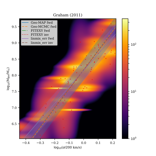
The approach in Section 3.3 presents a symmetric Bayesian solution to fitting a linear relation between two observables, incorporating heteroscedastic errors, upper limits and intrinsic scatter. As such, we would expect it to yield a non-biased estimate of the intrinsic slope of the relation (69), regardless of which way the relation is fit. To investigate this, the three datasets used in Table 1 of Park et al. (2012) were analysed. The data are originally from Gültekin et al. (2009), McConnell et al. (2011) and Graham et al. (2011). In order to compare with the results in Park et al. (2012), the measurement errors were modelled as uncorrelated bivariate Gaussians in the logarithmic space, leaving out all upper limits. Following Park et al. (2012), the standard deviations were set equal to mean errors, i.e. and similarly for the velocity dispersions. In addition, for the Graham et al. (2011) sample, which lacks velocity dispersion error data, the velocity dispersion errors were set to 10% and then propagated to averaged logarithmic errors. Finally, a dataset compiled from a multitude of sources used in van den Bosch (2016) was used. For this dataset, the errors were used as given, and upper limits were also incorporated in the fit.
For each dataset, the values for the same set of parameters as in Park et al. (2012) were computed: the intercept , slope and intrinsic scatter along the -axis . The results were computed for forward regression, equation (69), as well as the inverse regression, converting back to equivalent forward values in the end. The parameter values and uncertainties were estimated using the posterior distribution, equation (37), in two complementary ways.
The first set of estimates (Geo-MAP, hereafter), were derived by numerically maximizing the posterior distribution combined with a bootstrap resampling procedure. For each dataset, a total of bootstrap samples were constructed (Babu & Singh, 1983; Feigelson & Babu, 2012), where is the number of data points. The parameters were then estimated using the median parameter values. Parameter uncertainties at 1- level were estimated using median absolute deviations scaled to correspond to standard deviations for a normal distribution.
For the second set of estimates (Geo-MCMC, hereafter), the posterior distribution was sampled with the Markov chain Monte Carlo (MCMC) sampler emcee (Foreman-Mackey et al., 2013). Convergence during sampling was monitored with the potential scale reduction factor (Gelman et al., 2013), and sampling was continued until was achieved. The parameter estimates were obtained as the values corresponding to the sample with maximum posterior probability. The parameter uncertainties at 1- level were then estimated by constructing credible regions containing of the posterior probability mass. This was done by starting from the maximum posterior probability sample, and descending in posterior probability until the limit was exceeded. The extent of the credible region in each parameter direction was then used to compute the upper and lower 1- limits.
The results of this analysis are displayed in Table 2. Shown also are the results from Park et al. (2012) containing both forward and inverse regressions with the FITEXY (Press et al., 1992; Tremaine et al., 2002) and ‘Bayesian’ (i.e. linmix_err) methods. In addition, fits for the van den Bosch (2016) dataset without upper limits were computed separately for all methods. A graphical representation of the datasets and the relations obtained with the different methods is shown in Figure 5.
| Method | Intercept | Slope | a | a |
| Gültekin et al. (2009) data | ||||
| FITEXY fwd | ||||
| FITEXY inv | ||||
| linmix_err fwd | ||||
| linmix_err inv | ||||
| Geo-MAP fwd | ||||
| Geo-MCMC fwd | ||||
| McConnell et al. (2011) data | ||||
| FITEXY fwd | ||||
| FITEXY inv | ||||
| linmix_err fwd | ||||
| linmix_err inv | ||||
| Geo-MAP fwd | ||||
| Geo-MCMC fwd | ||||
| Graham et al. (2011) data | ||||
| FITEXY fwd | ||||
| FITEXY inv | ||||
| linmix_err fwd | ||||
| linmix_err inv | ||||
| Geo-MAP fwd | ||||
| Geo-MCMC fwd | ||||
| van den Bosch (2016) data | ||||
| linmix_err fwdb | ||||
| Geo-MAP fwd | ||||
| Geo-MCMC fwd | ||||
| van den Bosch (2016) data, no upper limits | ||||
| FITEXY fwd | c | |||
| FITEXY inv | c | |||
| linmix_err fwd | ||||
| linmix_err inv | ||||
| Geo-MAP fwd | ||||
| Geo-MCMC fwd | ||||
Notes.
a The orthogonal intrinsic scatter has been
converted to intrinsic scatter along the coordinate via the
equation (43) for both Geo methods.
Similarly, the scatter in -direction,
, has
been converted to equivalent orthogonal intrinsic scatter via the same
equation for the linmix_err and FITEXY methods.
b The linmix_err method only supports upper limits on the
dependent variable. As such, inverse fits cannot be computed.
c The FITEXY method does not give error estimates for the intrinsic
scatter.
 |
 |
 |
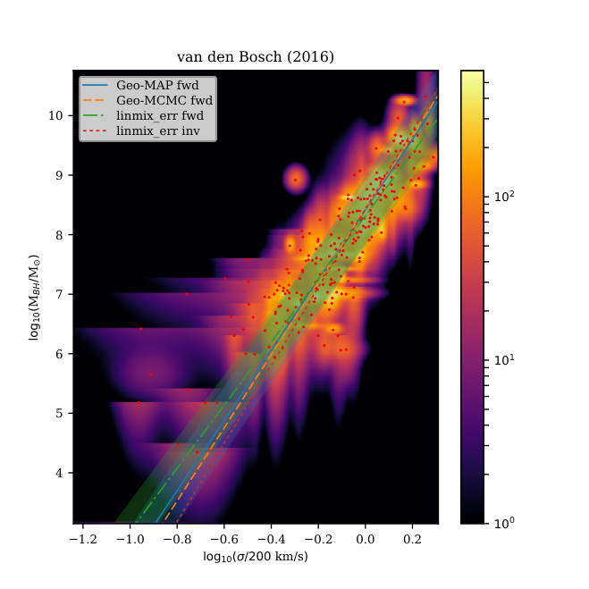 |
Table 2 indicates that the results computed using the geometrical approach presented in this paper are more consistent with the inverse fits done using the linmix_err and FITEXY algorithms. This is not surprising in light of the discussion in the previous section, since the slope of the – relation is high and we expect the forward fits to be biased towards low slopes in this situation. The effects of this bias can also be seen from the best-fitting values of the orthogonal intrinsic scatter, , for which the forward fits yield consistently higher values than the inverse fits for linmix_err and FITEXY. It seems that in these methods the lower value for the slope is compensated by a higher estimate for the intrinsic scatter. Note that this behaviour cannot be appreciated by looking at the values of the scatter in -direction, , since these are not truly intrinsic, but depend on and indeed show opposite behaviour. In contrast, the geometric methods yield identical results (up to sampling noise) in forward and inverse directions, so only forward results are shown in Table 2. The geometric methods also give consistently smaller estimates for the orthogonal intrinsic scatter. The 1- errors for all parameters are in general comparable between the methods, with the exception of the fully Bayesian MCMC approach, which consistently gives more conservative 1- errors.
Finally, it seems that if there indeed is a fundamental approximately linear relation between the logarithms of the mass of a supermassive black hole mass and the velocity dispersion of its host galaxy, the slope of the relation is likely to be , at least based on the van den Bosch (2016) data, which is the most comprehensive dataset used here. This is in contrast to the values around – often obtained in the literature (e.g. , Ferrarese & Merritt 2000; , Gebhardt et al. 2000; , Tremaine et al. 2002; , Gültekin et al. 2009; , McConnell & Ma 2013), including the value derived in van den Bosch (2016). These values were all derived using a method or a variation of a method described in Section 3.3.1, fitting the – relation in the ‘forward’ direction ( as a function of ), in which it has a high numerical value for the slope. This then causes the fitted value of the slope to be biased towards lower values. However, as can be seen from Figure 5, the numerically rather different estimates of the slope are not visually at all that obvious, with a change in slope of to corresponding only to a change in angle of the regression line with respect to a fixed direction, such as the -axis.
The obtained slope also crucially depends on the observational and other biases the data may have. Indeed, it is evident from Table 2 that the choice of dataset has an effect that is roughly comparable to the effect of the choice of method. It should also be noted that the fundamental relation, if there is one, may involve more than two physical quantities or their measurable proxies, as suggested in van den Bosch (2016). Fitting relations to a sampled projection of this hyperplane would then in general yield a higher value for the intrinsic scatter and slope that is offset from the ‘true’ value. As such, there is an urgent need for more high-quality data in order to say much with any certainty regarding the slope of the – relation (or the possible multi-variable generalizations), its possible evolution with redshift, or whether it truly is linear across the entire range of black hole masses.
5 Summary
We have presented a mathematical formalism for representing physical relations as submanifolds of a Riemannian manifold of observables . In this geometric approach, intrinsic scatter in the relation can be accommodated with probability distributions defined on the normal spaces of . Given a probability distribution of data, and parameterizations of the relation and the intrinsic scatter distribution, the formalism then yields a Bayesian posterior probability for the parameters of the relation and the intrinsic scatter distribution, equation (11). The novelty of our formulation is that it fully accommodates arbitrary measurement errors, both left and right censored data (upper and lower limits, respectively), truncation (non-detections) and extends the concept of intrinsic scatter both to non-linear relations and relations that define a submanifold of codimension greater than one.
We have derived explicit analytic results for the likelihood and the posterior distribution first in the case where the postulated relation defines a linear -dimensional hyperplane. We then extended this result to the case where the relation defines an -dimensional affine subspace, for an arbitrary , a result we believe to be potentially highly useful for seeking out the most likely codimension of a correlation within a set of -dimensional data. Finally, we have derived the likelihood and posterior distribution in the case of a line in two dimensions, and discussed its implications at length. We also compared the results given by our method with two established methods widely used in astronomical literature, namely FITEXY and linmix_err. We demonstrated that our inherently symmetrical geometrical approach is preferable in situations where the data obeys a relation with a slope much larger or smaller than one, and measurement errors and intrinsic scatter are severe and equally important.
Finally, we used our method to fit the – relation, between the mass of a supermassive black hole in a galactic bulge, and the stellar velocity dispersion of the bulge, using several published datasets. We compared our results to the fits in the literature, and find that our results support a slope of , clearly higher than the slopes derived in the literature. We note that this difference is mainly due to the methods used to derive the literature results. We show that if these methods are used ‘in reverse’, to fit as a function of , and then inverting the slope, the results are in much better agreement with ours. This is due to the tendency of standard methods, such as FITEXY or linmix_err, which do not respect the geometric symmetry of the problem, to misestimate steep slopes in the presence of intrinsic scatter (see Section 3.3.1 for the discussion).
Acknowledgements
The author is most grateful to the anonymous referee for comments and ideas that have contributed to a much improved manuscript, as well as to Peter H. Johansson for extensive comments on the manuscript drafts. The numerical computations in this work have benefited from the Python libraries NumPy, SciPy and SymPy (van der Walt et al., 2011; Jones et al., 01; Meurer et al., 2017). The Figures have been rendered with the help of the Python library Matplotlib (Hunter, 2007). This work has made use of NASA’s Astrophysics Data System Bibliographic Services. The research for this publication was supported by the Academy of Finland grant no. 1274931.
References
- Akritas & Bershady (1996) Akritas M. G., Bershady M. A., 1996, ApJ, 470, 706
- Babu & Singh (1983) Babu G. J., Singh K., 1983, The Annals of Statistics, pp 999–1003
- Beifiori et al. (2012) Beifiori A., Courteau S., Corsini E. M., Zhu Y., 2012, MNRAS, 419, 2497
- Boggs et al. (1987) Boggs P. T., Byrd R. H., Schnabel R. B., 1987, SIAM Journal on Scientific and Statistical Computing, 8, 1052
- Boggs et al. (1988) Boggs P. T., Spiegelman C. H., Donaldson J. R., Schnabel R. B., 1988, Journal of Econometrics, 38, 169
- Booth & Schaye (2009) Booth C. M., Schaye J., 2009, MNRAS, 398, 53
- Broemeling & Broemeling (2003) Broemeling L., Broemeling A., 2003, Biometrika, 90, 728
- Calin & Udriste (2014) Calin O., Udriste C., 2014, Geometric Modeling in Probability and Statistics. Mathematics and Statistics, Springer International Publishing
- Choi et al. (2014) Choi E., Naab T., Ostriker J. P., Johansson P. H., Moster B. P., 2014, MNRAS, 442, 440
- Crane et al. (2013) Crane K., Weischedel C., Wardetzky M., 2013, ACM Trans. Graph., 32
- Di Matteo et al. (2005) Di Matteo T., Springel V., Hernquist L., 2005, Nature, 433, 604
- Di Matteo et al. (2008) Di Matteo T., Colberg J., Springel V., Hernquist L., Sijacki D., 2008, ApJ, 676, 33
- Feigelson & Babu (1992) Feigelson E. D., Babu G. J., 1992, ApJ, 397, 55
- Feigelson & Babu (2012) Feigelson E., Babu G., 2012, Modern Statistical Methods for Astronomy: With R Applications. Cambridge University Press
- Ferrarese & Merritt (2000) Ferrarese L., Merritt D., 2000, ApJ, 539, L9
- Foreman-Mackey et al. (2013) Foreman-Mackey D., Hogg D. W., Lang D., Goodman J., 2013, PASP, 125, 306
- Fraser et al. (2010) Fraser D. A. S., Reid N., Marras E., Yi G. Y., 2010, Journal of the Royal Statistical Society: Series B (Statistical Methodology), 72, 631
- Fujiki & Akaho (2009) Fujiki J., Akaho S., 2009, in 2009 IEEE 12th International Conference on Computer Vision Workshops, ICCV Workshops. pp 250–255, doi:10.1109/ICCVW.2009.5457693
- Gebhardt et al. (2000) Gebhardt K., et al., 2000, ApJ, 539, L13
- Gelman et al. (2013) Gelman A., Carlin J., Stern H., Dunson D., Vehtari A., Rubin D., 2013, Bayesian Data Analysis, Third Edition. Chapman & Hall/CRC Texts in Statistical Science, Taylor & Francis
- George & McCulloch (1993) George E. I., McCulloch R., 1993, Journal of Statistical Planning and Inference, 37, 169
- Graham (2016) Graham A. W., 2016, Galactic Bulges, 418, 263
- Graham et al. (2011) Graham A. W., Onken C. A., Athanassoula E., Combes F., 2011, MNRAS, 412, 2211
- Gull (1989) Gull S. F., 1989, in , Maximum Entropy and Bayesian Methods. Springer, pp 511–518
- Gültekin et al. (2009) Gültekin K., et al., 2009, ApJ, 698, 198
- Hogg et al. (2010) Hogg D. W., Bovy J., Lang D., 2010, preprint, (arXiv:1008.4686)
- Hunter (2007) Hunter J. D., 2007, Computing In Science & Engineering, 9, 90
- Isobe et al. (1990) Isobe T., Feigelson E. D., Akritas M. G., Babu G. J., 1990, ApJ, 364, 104
- Jaynes (1983) Jaynes E., 1983, in Rosenkrantz R. D., ed., , Vol. 158, E.T. Jaynes: Papers on probability, statistics and statistical physics. D. Reidel Publishing Company, Dordrecht, Holland, pp 190–209
- Jaynes (1991) Jaynes E. T., 1991, Straight Line Fitting – A Bayesian Solution, Unpublished, available online at http://bayes.wustl.edu/sfg/line.pdf
- Jaynes (2003) Jaynes E. T., 2003, Probability Theory - The Logic of Science. Cambridge University Press, Cambridge, United Kingdom
- Johansson et al. (2009a) Johansson P. H., Naab T., Burkert A., 2009a, ApJ, 690, 802
- Johansson et al. (2009b) Johansson P. H., Burkert A., Naab T., 2009b, ApJ, 707, L184
- Jones et al. (01 ) Jones E., Oliphant T., Peterson P., et al., 2001–, SciPy: Open source scientific tools for Python, http://www.scipy.org/
- Jupp & Kent (1987) Jupp P. E., Kent J. T., 1987, Journal of the Royal Statistical Society. Series C (Applied Statistics), 36, 34
- Kelly (2007) Kelly B. C., 2007, ApJ, 665, 1489
- Lee (2013) Lee J., 2013, Introduction to Smooth Manifolds. Graduate Texts in Mathematics, Springer New York
- Magorrian et al. (1998) Magorrian J., et al., 1998, AJ, 115, 2285
- Markwardt (2009) Markwardt C. B., 2009, in Bohlender D. A., Durand D., Dowler P., eds, Astronomical Society of the Pacific Conference Series Vol. 411, Astronomical Data Analysis Software and Systems XVIII. p. 251 (arXiv:0902.2850)
- McConnell & Ma (2013) McConnell N. J., Ma C.-P., 2013, ApJ, 764, 184
- McConnell et al. (2011) McConnell N. J., Ma C.-P., Gebhardt K., Wright S. A., Murphy J. D., Lauer T. R., Graham J. R., Richstone D. O., 2011, Nature, 480, 215
- Meurer et al. (2017) Meurer A., et al., 2017, PeerJ Computer Science, 3, e103
- Novak et al. (2006) Novak G. S., Faber S. M., Dekel A., 2006, ApJ, 637, 96
- Park et al. (2012) Park D., Kelly B. C., Woo J.-H., Treu T., 2012, ApJS, 203, 6
- Pearson (1901) Pearson K., 1901, Philosophical Magazine Series 6, 2, 559
- Pennec (2006) Pennec X., 2006, J. Math. Imaging Vis., 25, 127
- Press et al. (1992) Press W. H., Teukolsky S. A., Vetterling W. T., Flannery B. P., 1992, Numerical recipes in FORTRAN. The art of scientific computing. Cambridge: University Press, c1992, 2nd ed.
- Robotham & Obreschkow (2015) Robotham A. S. G., Obreschkow D., 2015, Publ. Astron. Soc. Australia, 32, e033
- Saglia et al. (2016) Saglia R. P., et al., 2016, ApJ, 818, 47
- Sijacki et al. (2007) Sijacki D., Springel V., Di Matteo T., Hernquist L., 2007, MNRAS, 380, 877
- Sijacki et al. (2015) Sijacki D., Vogelsberger M., Genel S., Springel V., Torrey P., Snyder G. F., Nelson D., Hernquist L., 2015, MNRAS, 452, 575
- Stigler (1981) Stigler S. M., 1981, Ann. Statist., 9, 465
- Tremaine et al. (2002) Tremaine S., et al., 2002, ApJ, 574, 740
- Williams et al. (2010) Williams M. J., Bureau M., Cappellari M., 2010, MNRAS, 409, 1330
- Wolf & Zierau (1996) Wolf J. A., Zierau R., 1996, Riemannian exponential maps and decompositions of reductive Lie groups. Springer, pp 349–354
- Zellner (1971) Zellner A., 1971, An introduction to Bayesian inference in econometrics. Wiley series in probability and mathematical statistics: Applied probability and statistics, J. Wiley
- van den Bosch (2016) van den Bosch R. C. E., 2016, ApJ, 831, 134
- van der Walt et al. (2011) van der Walt S., Colbert S. C., Varoquaux G., 2011, Computing in Science Engineering, 13, 22
Appendix A Derivation of the posterior distribution
We present a derivation of the likelihood, equation (10), and the posterior distribution, equation (11), following the Bayesian style promoted in Jaynes (2003). We consider the following propositions:
- •
= ‘the true value of the observable is ’
- •
= ‘a value was measured for the observable’
- •
= ‘a detection was made’
- •
= ‘the true value of the observable is drawn from the distribution defined on a relation , with parameters and , respectively’
In addition, we will use to specify all the other relevant prior information. This includes the prior distribution of and , the measurement error distribution and the fact that the probability of a detection for a value of the observable is given by .
At the outset, we then know the following probabilities
| (70) | ||||
| (71) | ||||
| (72) |
We will need the probability of a measured value, given a true value and the fact that there is a detection. This is obtained with Bayes’ theorem
| (73) |
as a function of (which we write as in the following), since the prior probabilities and must be uninformative and equal everywhere, since nothing in tells us where the true and measured values are a priori.
We can now compute the probability of a measured value given the true value, yielding
| (74) |
where is the negation of (i.e. there was no detection). Here we used the fact that and form a complete () and independent set of propositions, together with the identity .
Using Bayes’ theorem again we can now obtain the probability that the data obey the relation and are drawn from , given the measured value. The theorem gives
| (75) |
Since the also form a complete and independent set of propositions (the true value must be somewhere, and the possible positions are independent), we can write
| (76) |
which gives the likelihood, equation (10). The factor is the parameter prior probability, and the denominator is a normalizing constant, given formally by
| (77) |
We then have the posterior probability, equation (11),
| (78) |
Appendix B An example of limit distributions
Here we present a simple example of how the framework presented in the paper works with upper limits, and how analytic results can be obtained for upper limits as well. This is desirable since typically the analytic expression for the likelihood is much faster to compute than performing a numerical integration to obtain the required value. As mentioned in Section 2.3, limits are taken into account by including them into the measurement error distribution. This can be done for the examples in Sections 3.1–3.3 by substituting one or more degrees of freedom in equations (16) and (32) with suitable one-dimensional distributions. Conceptually the simplest possibility is the uniform distribution, so that
| (79) |
where if and otherwise, and is the limiting value. Other choices with less pronounced cutoffs are naturally also possible. If the measurements are already given in logarithmic units with base , the form
| (80) |
must be used instead. Lower limits can be introduced in an analogous manner.
Analytic results of reasonable complexity based on these limit distributions can be obtained for the example in Section 3.3. For the linear case we have
| (81) |
| (82) |
for the upper limits in and directions respectively, where and are the corresponding limiting values. If the measurements have been given in logarithmic scale with base , we have instead
| (83) |
| (84) |
where . Note that here the limiting values and are given in linear scale. For numerical applications, it should be noted that the arguments of the -exponential and the function may have large numerical values, and asymptotic expansions should be used when necessary.