跳到论文正文
W Papers独立论文阅读器 arXiv:1704.05461 论文正文 计算阅读时间 · 0%
引用这篇论文根据当前论文元数据生成,正式投稿前建议核对。


License: arXiv.org perpetual non-exclusive license
arXiv:1704.05461v2 [hep-th] 28 Apr 2017

Quantum critical response: from conformal perturbation theory to holography

Andrew Lucas Affiliation: Department of Physics, Stanford University, Stanford, CA 94305, USA Email: ajlucas@stanford.edu    Todd Sierens Affiliation: Perimeter Institute for Theoretical Physics, Waterloo, Ontario N2L 2Y5, Canada Affiliation: Department of Physics & Astronomy and Guelph-Waterloo Physics Institute, University of Waterloo, Waterloo, Ontario N2L 3G1, Canada Email: tsierens@perimeterinstitute.ca    and William Witczak-Krempa Affiliation: Department of Physics and Regroupement québéquois sur les matériaux de pointe, Université de Montréal, Montréal, Québec, H3C 3J7, Canada Email: w.witczak-krempa@umontreal.ca
Abstract

We discuss dynamical response functions near quantum critical points, allowing for both a finite temperature and detuning by a relevant operator. When the quantum critical point is described by a conformal field theory (CFT), conformal perturbation theory and the operator product expansion can be used to fix the first few leading terms at high frequencies. Knowledge of the high frequency response allows us then to derive non-perturbative sum rules. We show, via explicit computations, how holography recovers the general results of conformal field theory, and the associated sum rules, for any holographic field theory with a conformal UV completion – regardless of any possible new ordering and/or scaling physics in the IR. We numerically obtain holographic response functions at all frequencies, allowing us to probe the breakdown of the asymptotic high-frequency regime. Finally, we show that high frequency response functions in holographic Lifshitz theories are quite similar to their conformal counterparts, even though they are not strongly constrained by symmetry.

1 Introduction

A quantum critical point (QCP) is a zero-temperature continuous phase transition which arises as a coupling parameter is tuned through a critical value. Typically, one finds that at zero temperature (away from the QCP) there are two distinct ‘conventional’ gapped or gapless phases of matter, whereas at finite temperature there is a finite region of the phase diagram dominated strongly by critical fluctuations: see Figure 1. A canonical example is the transverse field quantum Ising model in D=1+1,2+1D=1+1,2+1 and 3+13+1 spacetime dimensions, where the QCP separates a paramagnet from a broken symmetry phase, the ferromagnet. The QCP is described at low energies by the DD-dimensional Ising CFT [1]. Other examples involve fermions such as the Gross-Neveu model [2, 1], and/or gauge fields (e.g. Banks-Zaks fixed points [3]).

Figure 1: Schematic phase diagram of a theory with a (conformal) quantum critical point separating two phases at zero temperature. The non-thermal detuning parameter hh must be set to zero at the critical point. At finite temperature TT, when T≳|h|1D−Δ=|h|νT\gtrsim|h|^{\frac{1}{D-\Delta}}=|h|^{\nu}, there is a window in between the two phases where the system behaves qualitatively like the quantum critical point h=0h=0, detuned only by temperature. In this paper, we demonstrate that certain fingerprints in the dynamical response functions of the quantum critical point can extend throughout this entire phase diagram.

Proximity to a QCP is believed to be the origin of exotic response functions in many experimentally interesting condensed matter systems [4]. Even when the ground state is conventional, so long as it lies ‘near’ a QCP, both thermodynamic and dynamical response functions are significantly modified by quantum critical fluctuations. Because interesting quantum critical theories are strongly coupled and lack long-lived quasiparticle excitations, obtaining quantitative predictions for critical dynamical response functions, where both quantum and thermal fluctuations must be accounted for, has proven to be challenging. In this respect, quantum Monte Carlo studies have proven useful to obtain the response functions in imaginary time [5, 6, 7, 8, 9]. The precise analytic continuation to real frequencies of such data constitutes a difficult open problem. The results of this paper impose constraints on the response functions that will constrain the continuation procedure.

In the case of conformal field theories (CFTs), one can derive rigorous and general constraints on the dynamics at zero and finite temperature by using the operator product expansion (OPE). In addition, one can study the response functions in the neighborhood of the QCP by using conformal perturbation theory, where the expansion parameter is the detuning of the coupling parameter from its critical value. Another technique is the gauge-gravity duality [10], which relates certain large-NN matrix quantum field theories to classical gravity theories in higher dimensional spacetimes. The power of this approach is that we are very easily able to access finite temperature and finite frequency response functions, directly in real time. Unfortunately, experimentally realized condensed matter systems do not have weakly coupled gravity duals, and some care is required in identifying which features of these holographic theories are relevant for broader field theories.

In this paper, we will discuss the asymptotics of a variety of response functions at high frequency [11, 12, 13, 5, 14, 15, 16, 8, 17, 18, 19, 20]. We will show that in holographic field theories, this asymptotics is universal and does not depend in any detailed fashion on the nature of the ground state. As a consequence, we will then derive non-perturbative sum rules which may be tested directly in experiments. In the special case when the QCP is a conformal field theory (CFT), we will also be able to compare our holographic calculation of the response functions with an independent computation using techniques of conformal field theory, and will find perfect agreement. We will also discuss the generalization of these calculations to a richer class of Lifshitz field theories, which are less sharply constrained by symmetry.

1.1 Main Results

We study a quantum critical system in DD spacetime dimensions deformed by a relevant operator 𝒪\mathcal{O}:

S=SQCP−h​∫dD​x​𝒪,S=S_{\mathrm{QCP}}-h\int\mathrm{d}^{D}x\;\mathcal{O}, (1)

where for simplicity we have chosen the coupling hh to be xx-independent. We briefly discuss the case of an inhomogeneous coupling in the conclusion 8. This formula is presented in real time; in Euclidean time, there is a relative minus sign for the second term. Now, let Δ\Delta be the scaling dimension of 𝒪\mathcal{O}:

⟨𝒪⁡(𝐱,t)​𝒪​(𝐲,t)⟩0=C𝒪​𝒪​|𝐱−𝐲|−2​Δ,\langle\mathcal{O}(\mathbf{x},t)\mathcal{O}(\mathbf{y},t)\rangle_{0}=C_{\mathcal{OO}}|\mathbf{x}-\mathbf{y}|^{-2\Delta}, (2)

where the 00 subscript means that the correlation function is evaluated at the QCP T=h=0T=h=0. The parameter hh is commonly called the (non-thermal) detuning parameter; it drives the quantum phase transition. We also will study this detuned theory at finite temperature TT. The dynamical critical exponent zz of this QCP is defined as the ‘dimension’ of energy: namely, a dilation of space 𝐱→λ​𝐱\mathbf{x}\to\lambda\mathbf{x} is accompanied by a temporal dilation t→λz​tt\to\lambda^{z}t in order to be a symmetry. This implies that the excitations of this theory (generally there are no well-defined quasi-particles at the QCP) disperse as ω⁡(q)∼qz\omega(q)\sim q^{z}. For simplicity, in much of this paper we will focus on the case z=1z=1, specializing to the case where the QCP is a conformal field theory, returning to the more general case z≠1z\neq 1 at the end of the paper.

Let 𝒳\mathcal{X} be a local operator of scaling dimension Δ𝒳\Delta_{\mathcal{X}} in this critical theory, and assume for now that Δ𝒳≠(D/2)+n\Delta_{\mathcal{X}}\neq(D/2)+n, where nn is an integer, which is the generic case and ensures that both powers in the brackets do not differ by an integer (otherwise, additional logarithms can appear). We will show that, when z=1z=1, the generic asymptotic expansion of the dynamical response function ⟨𝒳​𝒳⟩\langle\mathcal{XX}\rangle at high frequency is:

⟨𝒳⁡(ω)​𝒳​(−ω)⟩=(i​ω)2​Δ𝒳−D​[𝒞𝒳​𝒳+𝒜​h(i​ω)D−Δ+ℬ​⟨𝒪⟩(i​ω)Δ+⋯],\langle\mathcal{X}(\omega)\mathcal{X}(-\omega)\rangle=(\mathrm{i}\omega)^{2\Delta_{\mathcal{X}}-D}\left[\mathcal{C}_{\mathcal{XX}}+\mathcal{A}\frac{h}{(\mathrm{i}\omega)^{D-\Delta}}+\mathcal{B}\frac{\langle\mathcal{O}\rangle}{(\mathrm{i}\omega)^{\Delta}}+\cdots\right], (3)

where ⟨⋯⟩\langle\cdots\rangle denotes an expectation value evaluated at non-zero values of hh and TT, in contrast to ⟨⋯⟩0\langle\cdots\rangle_{0}, which is evaluated directly in the quantum critical theory, at h=T=0h=T=0. We emphasize that the first correction is analytic in the coupling hh and independent of temperature. The expansion (3) holds when ω≫T,|h|1/(D−Δ)\omega\gg T,|h|^{1/(D-\Delta)} (ℏ=kB=1\hbar=k_{\mathrm{B}}=1) and when the detuned system has a finite correlation length. It can fail in regions separated from the quantum critical “fan” by a phase transition, where potentially new gapless modes can arise. An example of this failure was shown in the broken symmetry (Goldstone) phase in the vicinity of the Wilson-Fisher O⁡(N)O(N) QCP at large NN [20]. The leading order coefficient 𝒞𝒳​𝒳\mathcal{C}_{\mathcal{XX}} is an operator normalization in the vacuum of the CFT. We compute the coefficients 𝒜\mathcal{A} and ℬ\mathcal{B} exactly for arbitrary spacetime dimension DD and dimension Δ\Delta of the (relevant) operator, in three practical examples: ⟨𝒪0​𝒪0⟩\langle\mathcal{O}_{0}\mathcal{O}_{0}\rangle, ⟨Jx​Jx⟩\langle J^{x}J^{x}\rangle, and ⟨Tx​y​Tx​y⟩\langle T^{xy}T^{xy}\rangle. Here 𝒪0\mathcal{O}_{0} is a scalar operator, JxJ^{x} is a spatial component of a conserved current, and Tx​yT^{xy} is an off-diagonal spatial component of the conserved stress-energy tensor. Remarkably, 𝒜\mathcal{A} and ℬ\mathcal{B} will not depend on either hh or TT, and are properties of the pure CFT, and the choice of operator 𝒳\mathcal{X}. Furthermore, the ratio 𝒜/ℬ\mathcal{A}/\mathcal{B} is universal, depending only on Δ\Delta and DD.

CFT operator 𝒳\mathcal{X} 𝒜/ℬ\mathcal{A}/\mathcal{B}
Tx​yT_{xy} (stress tensor) (45)
JxJ_{x} (conserved current) (37)
𝒪0\mathcal{O}_{0} (scalar operator) (22)
Table 1: Where to find our main results for the ratio of coefficients 𝒜/ℬ\mathcal{A}/\mathcal{B} in the asymptotic expansion of ⟨𝒳​𝒳⟩\langle\mathcal{X}\mathcal{X}\rangle in CFTs, (3).

When Δ𝒳\Delta_{\mathcal{X}} and/or Δ𝒳−Δ\Delta_{\mathcal{X}}-\Delta is an integer or half-integer, depending on the dimension DD, logarithmic corrections to (3) appear. These special cases are important because conserved currents have such dimensions, and we will discuss them later in this paper.

The reason that 𝒪\mathcal{O} be a relevant operator is to ensure that the asymptotic expansion (3) is well-behaved; if 𝒪\mathcal{O} is irrelevant, the second term in (3) dominates. This is not surprising, as we are probing the UV physics (which is sensitive to the dynamics of irrelevant operators).

One of the main purposes of the asymptotic expansion (3) is to verify when the following kind of sum rule holds:

∫0∞d​ω​Re​(⟨𝒳⁡(−ω)​𝒳​(ω)⟩i​ω−𝒞𝒳​𝒳⋅(i​ω)2​Δ𝒳−D)=0.\int\limits_{0}^{\infty}\mathrm{d}\omega\;\mathrm{Re}\left(\frac{\langle\mathcal{X}(-\omega)\mathcal{X}(\omega)\rangle}{\mathrm{i}\omega}-\mathcal{C}_{\mathcal{XX}}\cdot(\mathrm{i}\omega)^{2\Delta_{\mathcal{X}}-D}\right)=0. (4)

Clearly, this sum rule is automatically satisfied at the critical point, but it can also be satisfied off-criticality. When h=0h=0, we will see that such a sum rule will only hold if 2​Δ𝒳−D<Δ2\Delta_{\mathcal{X}}-D<\Delta. When h≠0h\neq 0, an additional inequality Δ<2​(D−Δ𝒳)\Delta<2(D-\Delta_{\mathcal{X}}) is also required.

Eq. (3) is presented in real time. Our derivation of this result will occur in Euclidean time. It is usually straightforward to analytically continue back to real time. There can be subtleties for certain values of DD and Δ\Delta, for certain operators 𝒳\mathcal{X}, and we will clarify the restrictions later.

We will present two derivations of (3): one using conformal perturbation theory applied to general CFTs (such an approached was succinctly presented for the conductivity in [20]), one using holography. We will show that these approaches exactly agree. A priori, as the conformal perturbation theory approach does not rely on the large-NN matrix limit of holography, it may seem as though the holographic derivation is superfluous. However, we will argue that this is not the case: that conformal perturbation theory is completely controlled at finite hh and finite TT is not always clear, especially if the ground state of the detuned theory is not a conventional gapped phase. Our holographic computation reveals that, independent of the details of the ground state, the asymptotics of the response functions are given by (3), with all coefficients in the expansion determined completely by the UV CFT. We expect that – with some important exceptions in broken symmetry phases [20] – this is a robust result of our analysis, valid beyond the large-NN limit.

For holographic models, we will also study the case z≠1z\neq 1, and find a simple generalization of (3). While we will prove the universality of (3) even beyond holography when z=1z=1, we cannot prove this universality for z≠1z\neq 1.

We also present the full frequency dependence of these response functions in multiple holographic models. In addition to verifying that the asymptotics (3) and the associated sum rules such as (4) hold, we will be able to probe frequency scales past which conformal perturbation theory fails, both at a finite temperature critical point, and in systems strongly detuned off-criticality.

1.2 Outline

The remainder of the paper is organized as follows. In Section 2, we will describe the asymptotics of response functions using conformal perturbation theory. In Section 3, we will describe a very general class of holographic theories with conformal UV completions, and compute all necessary CFT data required to compare with Section 2. Section 4 contains a direct computation of high frequency holographic response functions, in which exact agreement with conformal perturbation theory is found. We numerically compute the full frequency response functions in Section 5. We generalize our approach in Section 6 to holographic theories with ‘Lifshitz’ field theory duals, where there are, as of yet, no other approaches like conformal field theory which can be used. We discuss sum rules in Section 7. We conclude the paper by discussing the possible breakdown of (3) in broken symmetry phases, and the generalization of (3) to QCPs deformed by disorder.

2 Conformal Perturbation Theory

In this section, we present a computation of the high-frequency asymptotic behavior of the three advertised two-point functions, ⟨𝒪0​𝒪0⟩\langle\mathcal{O}_{0}\mathcal{O}_{0}\rangle, ⟨Jx​Jx⟩\langle J^{x}J^{x}\rangle, ⟨Tx​y​Tx​y⟩\langle T^{xy}T^{xy}\rangle, using conformal perturbation theory for generic spacetime dimension DD. The computation of ⟨Jx​Jx⟩\langle J^{x}J^{x}\rangle was recently presented by two of us [20]. We will present the computation of ⟨𝒪0​𝒪0⟩\langle\mathcal{O}_{0}\mathcal{O}_{0}\rangle in detail – the computation of the latter two is extremely similar, and so we simply summarize the results.

2.1 Scalar Two-Point Functions

We begin with the correlator ⟨𝒪0​𝒪0⟩\langle\mathcal{O}_{0}\mathcal{O}_{0}\rangle of a scalar operator 𝒪0\mathcal{O}_{0} with dimension Δ0\Delta_{0}. In the vacuum of a unitary CFT, one finds that in position space

⟨𝒪0​(x)​𝒪0​(y)⟩0=C𝒪0​𝒪0|x−y|2​Δ0.\langle\mathcal{O}_{0}(x)\mathcal{O}_{0}(y)\rangle_{0}=\frac{C_{\mathcal{O}_{0}\mathcal{O}_{0}}}{|x-y|^{2\Delta_{0}}}. (5)

In this work, we are interested in momentum space correlation functions, which are readily computed (up to an overall δ\delta function):

⟨𝒪0​(k)​𝒪0​(−k)⟩0\displaystyle\langle\mathcal{O}_{0}(k)\mathcal{O}_{0}(-k)\rangle_{0} =∫dD​x​ei​k⋅x​⟨𝒪0​(x)​𝒪0​(0)⟩0=∫0∞d​ss​∫dD​x​ei​k⋅x−s​x2​sΔ0Γ⁡(Δ0)​C𝒪0​𝒪0\displaystyle=\int\mathrm{d}^{D}x\,\mathrm{e}^{\mathrm{i}k\cdot x}\langle\mathcal{O}_{0}(x)\mathcal{O}_{0}(0)\rangle_{0}=\int\limits_{0}^{\infty}\frac{\mathrm{d}s}{s}\int\mathrm{d}^{D}x\mathrm{e}^{\mathrm{i}k\cdot x-sx^{2}}\frac{s^{\Delta_{0}}}{\Gamma(\Delta_{0})}C_{\mathcal{O}_{0}\mathcal{O}_{0}}
=2D−2​Δ​πD/2​Γ​(D2−Δ0)Γ⁡(Δ0)​C𝒪0​𝒪0​k2​Δ0−D≡𝒞𝒪0​𝒪0​k2​Δ0−D.\displaystyle=\frac{2^{D-2\Delta}\pi^{D/2}\Gamma(\frac{D}{2}-\Delta_{0})}{\Gamma(\Delta_{0})}C_{\mathcal{O}_{0}\mathcal{O}_{0}}k^{2\Delta_{0}-D}\equiv\mathcal{C}_{\mathcal{O}_{0}\mathcal{O}_{0}}k^{2\Delta_{0}-D}. (6)

If Δ0−D2=0,1,2,…\Delta_{0}-\frac{D}{2}=0,1,2,\ldots is an integer, then we find an extra factor of log⁡k\log k in (6); henceforth in the main text, we will assume that Δ0−D2\Delta_{0}-\frac{D}{2} is not an integer. We also note that C𝒪0​𝒪0>0C_{\mathcal{O}_{0}\mathcal{O}_{0}}>0, but depending on Δ\Delta and DD, 𝒞𝒪0​𝒪0\mathcal{C}_{\mathcal{O}_{0}\mathcal{O}_{0}} can take either sign.

We can now deform away from the exact critical point by turning on a finite temperature TT or detuning hh. (6) will now receive corrections due to hh and TT – the leading order corrections are written in (3). We first outline the argument for how the structure (3) arises, after which it will be relatively straightforward to do a direct computation to fix 𝒜\mathcal{A} and ℬ\mathcal{B}. Suppose that we set T=0T=0, for simplicity, but detune our CFT by hh, (1). We express the expectation value using a Euclidean path integral:

⟨𝒪0​(Ω)​𝒪0​(−Ω)⟩h\displaystyle\langle\mathcal{O}_{0}(\Omega)\mathcal{O}_{0}(-\Omega)\rangle_{h} =1𝒵⁡[h]​∫D​ΦCFT​e−SCFT+h​𝒪​(0)​𝒪0​(Ω)​𝒪0​(−Ω)\displaystyle=\frac{1}{\mathcal{Z}[h]}\int\mathrm{D}\Phi_{\mathrm{CFT}}\mathrm{e}^{-S_{\mathrm{CFT}}+h\mathcal{O}(0)}\mathcal{O}_{0}(\Omega)\mathcal{O}_{0}(-\Omega)
=𝒵⁡[0]𝒵⁡[h]​⟨𝒪0​(Ω)​𝒪0​(−Ω)​eh​𝒪​(0)⟩0\displaystyle=\frac{\mathcal{Z}[0]}{\mathcal{Z}[h]}\left\langle\mathcal{O}_{0}(\Omega)\mathcal{O}_{0}(-\Omega)\mathrm{e}^{h\mathcal{O}(0)}\right\rangle_{0}
=⟨𝒪0​(Ω)​𝒪0​(−Ω)​(1+h​𝒪​(0)+⋯)⟩0\displaystyle=\left\langle\mathcal{O}_{0}(\Omega)\mathcal{O}_{0}(-\Omega)(1+h\mathcal{O}(0)+\cdots)\right\rangle_{0}
=𝒞𝒪0​𝒪0​Ω2​Δ0−D+𝒜​hΩD−Δ​Ω2​Δ0−D+⋯\displaystyle=\mathcal{C}_{\mathcal{O}_{0}\mathcal{O}_{0}}\Omega^{2\Delta_{0}-D}+\frac{\mathcal{A}h}{\Omega^{D-\Delta}}\Omega^{2\Delta_{0}-D}+\cdots (7)

Here 𝒪⁡(0)\mathcal{O}(0) is the zero momentum mode of 𝒪\mathcal{O}. The first term of (7) follows from (6). The power of Ω\Omega in the second term has been fixed by dimensional analysis; below we explicitly evaluate this term by evaluating the 3-point function ⟨𝒪0​𝒪0​𝒪⟩0\langle\mathcal{O}_{0}\mathcal{O}_{0}\mathcal{O}\rangle_{0}. This 3-point function is fixed by the conformal Ward identities in momentum space up to an overall coefficient; alternatively, one can perform an analytic continuation from position to momentum space, although one must be careful with regularization [21]. Holography naturally produces the correct answer as we show below. There are further terms in (7) containing subleading integer powers of h/ΩD−Δh/\Omega^{D-\Delta}.

However, the 𝒪0\mathcal{O}_{0} 2-point correlation function will also contain terms non-analytic in h/ΩD−Δh/\Omega^{D-\Delta}. It will often be the case, in the pure CFT, that the operator product expansion (OPE) will take the form, here expressed in momentum-space:

𝒪0​(Ω)​𝒪0​(−Ω)=𝒞𝒪0​𝒪0​Ω2​Δ0−D+ℬ​Ω2​Δ0−D​𝒪⁡(0)ΩΔ+⋯\mathcal{O}_{0}(\Omega)\mathcal{O}_{0}(-\Omega)=\mathcal{C}_{\mathcal{O}_{0}\mathcal{O}_{0}}\Omega^{2\Delta_{0}-D}+\mathcal{B}\Omega^{2\Delta_{0}-D}\frac{\mathcal{O}(0)}{\Omega^{\Delta}}+\cdots (8)

We have ⟨𝒪⟩0=0\langle\mathcal{O}\rangle_{0}=0, since the pure CFT has no dimensionful parameter. Hence, upon averaging this equation in a CFT, the ℬ\mathcal{B} contribution to the OPE vanishes. However, once we detune with hh at T=0T=0, we expect:

⟨𝒪⟩h=A±​|h|ΔD−Δ,\langle\mathcal{O}\rangle_{h}=A_{\pm}|h|^{\frac{\Delta}{D-\Delta}}, (9)

with a coefficient that generally depends on the sign of hh. The OPE (8) is a high energy property of the theory, and should be valid even at finite hh, so long the frequency Ω\Omega is large enough: h≪ΩD−Δh\ll\Omega^{D-\Delta}. Hence, we expect that we may apply the expectation value to the local OPE and find an additional contribution to the two-point function, linear in ⟨𝒪⟩\langle\mathcal{O}\rangle:

⟨𝒪0​(Ω)​𝒪0​(−Ω)⟩h=𝒞𝒪0​𝒪0​Ω2​Δ0−D+𝒜​hΩD−Δ​Ω2​Δ0−D+⋯+ℬ​⟨𝒪⟩ΩΔ​Ω2​Δ0−D+⋯.\langle\mathcal{O}_{0}(\Omega)\mathcal{O}_{0}(-\Omega)\rangle_{h}=\mathcal{C}_{\mathcal{O}_{0}\mathcal{O}_{0}}\Omega^{2\Delta_{0}-D}+\frac{\mathcal{A}h}{\Omega^{D-\Delta}}\Omega^{2\Delta_{0}-D}+\cdots+\mathcal{B}\frac{\langle\mathcal{O}\rangle}{\Omega^{\Delta}}\Omega^{2\Delta_{0}-D}+\cdots. (10)

In the context of classical critical phenomena, an analogous expansion for the short-distance spatial correlators of the order parameter have been found for thermal Wilson-Fisher fixed points in D=3D=3 [22], and subsequently more quantitatively in other theories using the OPE [23, 24, 25]. These classical results are a special case of (10) analytically continued to imaginary times at T=0T=0. In the context of the classical 3D Ising model, such an expansion was recently used together with conformal bootstrap results to make predictions for the correlators of various scalars near the critical temperature TcT_{c} [25]. We also see that the coefficient ℬ\mathcal{B} is nothing more than an OPE coefficient in the CFT, as found in [8, 20].

Obviously, for generic Δ\Delta, the power of hh in (9) is not an integer. Hence, the ℬ\mathcal{B} term in this expansion cannot be captured at any finite order in the conformal perturbation theory expansion (7). Still, we will see that it is possible to compute the ratio 𝒜/ℬ\mathcal{A}/\mathcal{B} in terms of CFT data.

We claim that upon generalizing to finite temperature TT, the essential arguments above follow through, despite the fact that when T>0T>0, ⟨𝒪⟩\langle\mathcal{O}\rangle will be an analytic function of hh near h=0h=0. Our holographic computation will confirm this insight in a broad variety of models.

The argument above contains essentially all of the physics of conformal perturbation theory. It remains to explicitly fix the coefficient 𝒜\mathcal{A} in terms of ℬ\mathcal{B}. To do so, we carefully study the 3-point function ⟨𝒪0​(p1)​𝒪0​(p2)​𝒪​(p3)⟩0\langle\mathcal{O}_{0}(p_{1})\mathcal{O}_{0}(p_{2})\mathcal{O}(p_{3})\rangle_{0}, upon choosing the momenta to be

p1\displaystyle p_{1} =(Ω,0),\displaystyle=(\Omega,0), (11a)
p2\displaystyle p_{2} =(−Ω−p,0),\displaystyle=(-\Omega-p,0), (11b)
p3\displaystyle p_{3} =(p,0).\displaystyle=(p,0). (11c)

where p≪Ωp\ll\Omega. In a conformal field theory, this correlation function is completely fixed up to an overall prefactor A𝒪0​𝒪0​𝒪A_{\mathcal{O}_{0}\mathcal{O}_{0}\mathcal{O}} [21, 26]:

⟨𝒪0​(p1)​𝒪0​(p2)​𝒪​(p3)⟩0=A𝒪0​𝒪0​𝒪​I​(D2−1,Δ0−D2,Δ0−D2,Δ−D2)\langle\mathcal{O}_{0}(p_{1})\mathcal{O}_{0}(p_{2})\mathcal{O}(p_{3})\rangle_{0}=A_{\mathcal{O}_{0}\mathcal{O}_{0}\mathcal{O}}I\!\left(\tfrac{D}{2}-1,\Delta_{0}-\tfrac{D}{2},\Delta_{0}-\tfrac{D}{2},\Delta-\tfrac{D}{2}\right) (12)

where we have defined (for later convenience):

I⁡(a,b,c,d)≡∫0∞d​x​xa​p1b​p2c​p3d​Kb​(p1​x)​Kc​(p2​x)​Kd​(p3​x).I(a,b,c,d)\equiv\int\limits_{0}^{\infty}\mathrm{d}x\;x^{a}p_{1}^{b}p_{2}^{c}p_{3}^{d}\,\mathrm{K}_{b}(p_{1}x)\mathrm{K}_{c}(p_{2}x)\mathrm{K}_{d}(p_{3}x). (13)

Here Kν​(x)\mathrm{K}_{\nu}(x) is the modified Bessel function which exponentially decays as x→∞x\rightarrow\infty. From (11), we see that p1,2≫p3p_{1,2}\gg p_{3}. Hence, a good approximation to (13) should come from an asymptotic expansion of Kd​(p3​x)\mathrm{K}_{d}(p_{3}x) in (13). Defining

𝒵⁡(b)≡2b−1​Γ​(b)\mathcal{Z}(b)\equiv 2^{b-1}\Gamma(b) (14)

and using the asymptotic expansion

Kb​(x)=𝒵⁡(b)​x−b​[1+O⁡(x2)]+𝒵⁡(−b)​xb​[1+O⁡(x2)],\mathrm{K}_{b}(x)=\mathcal{Z}(b)x^{-b}\left[1+\mathrm{O}\left(x^{2}\right)\right]+\mathcal{Z}(-b)x^{b}\left[1+\mathrm{O}\left(x^{2}\right)\right], (15)

we take the limit of (11) and simplify (13) to

⟨𝒪0​(p1)​𝒪0​(p2)​𝒪​(p3)⟩0≈A𝒪0​𝒪0​𝒪​𝒵​(Δ−D2)​Ψ​(D−Δ,Δ0−D2)​Ω2​Δ0+Δ−2​D\displaystyle\langle\mathcal{O}_{0}(p_{1})\mathcal{O}_{0}(p_{2})\mathcal{O}(p_{3})\rangle_{0}\approx A_{\mathcal{O}_{0}\mathcal{O}_{0}\mathcal{O}}\mathcal{Z}\left(\Delta-\tfrac{D}{2}\right)\Psi\left(D-\Delta;\Delta_{0}-\tfrac{D}{2}\right)\Omega^{2\Delta_{0}+\Delta-2D}
+A𝒪0​𝒪0​𝒪​𝒵​(D2−Δ)​Ψ​(Δ,Δ0−D2)​p2​Δ−D​Ω2​Δ0−Δ−D,\displaystyle\;\;\;\;\;\;\;+A_{\mathcal{O}_{0}\mathcal{O}_{0}\mathcal{O}}\mathcal{Z}\left(\tfrac{D}{2}-\Delta\right)\Psi\left(\Delta;\Delta_{0}-\tfrac{D}{2}\right)p^{2\Delta-D}\Omega^{2\Delta_{0}-\Delta-D}, (16)

where we have defined

Ψ⁡(a,b)≡∫0∞d​x​xa−1​Kb​(x)2=π​Γ​(a2)​Γ​(a2+b)​Γ​(a2−b)4​Γ​(1+a2).\Psi(a;b)\equiv\int\limits_{0}^{\infty}\mathrm{d}x\;x^{a-1}\mathrm{K}_{b}(x)^{2}=\frac{\sqrt{\pi}\Gamma(\frac{a}{2})\Gamma(\frac{a}{2}+b)\Gamma(\frac{a}{2}-b)}{4\Gamma(\frac{1+a}{2})}. (17)

The first term of (16) is completely regular as p→0p\rightarrow 0. The correlation function ⟨𝒪0​(Ω)​𝒪0​(−Ω)​𝒪​(0)⟩0\langle\mathcal{O}_{0}(\Omega)\mathcal{O}_{0}(-\Omega)\mathcal{O}(0)\rangle_{0} which appeared in conformal perturbation theory in (7) should be interpreted as this first contribution. Thus we obtain

𝒜=A𝒪0​𝒪0​𝒪​𝒵​(Δ−D2)​Ψ​(D−Δ,Δ0−D2).\mathcal{A}=A_{\mathcal{O}_{0}\mathcal{O}_{0}\mathcal{O}}\mathcal{Z}\!\left(\Delta-\tfrac{D}{2}\right)\Psi\!\left(D-\Delta;\Delta_{0}-\tfrac{D}{2}\right). (18)

The second term of (16) can be interpreted as follows. At a small momentum pp, the OPE (8) generalizes to

𝒪0​(Ω)​𝒪0​(−Ω−p)=ℬ​Ω2​Δ0−D​𝒪⁡(−p)ΩΔ+⋯.\mathcal{O}_{0}(\Omega)\mathcal{O}_{0}(-\Omega-p)=\mathcal{B}\Omega^{2\Delta_{0}-D}\frac{\mathcal{O}(-p)}{\Omega^{\Delta}}+\cdots. (19)

Upon contracting both sides of (19) with ⟨⋯𝒪(p)⟩CFT\langle\cdots\mathcal{O}(p)\rangle_{\mathrm{CFT}}, we obtain a contribution which is non-analytic in pp:

⟨𝒪0​(p1)​𝒪0​(p2)​𝒪​(p3)⟩0\displaystyle\langle\mathcal{O}_{0}(p_{1})\mathcal{O}_{0}(p_{2})\mathcal{O}(p_{3})\rangle_{0} =⋯+ℬ​Ω2​Δ0−Δ−D​⟨𝒪⁡(−p)​𝒪​(p)⟩0\displaystyle=\cdots+\mathcal{B}\Omega^{2\Delta_{0}-\Delta-D}\langle\mathcal{O}(-p)\mathcal{O}(p)\rangle_{0}
=⋯+ℬ​𝒞0​p2​Δ−D​Ω2​Δ0−Δ−D.\displaystyle=\cdots+\mathcal{B}\mathcal{C}_{0}p^{2\Delta-D}\Omega^{2\Delta_{0}-\Delta-D}. (20)

Comparing (20) with (16) we conclude

ℬ​𝒞𝒪​𝒪=A𝒪0​𝒪0​𝒪​𝒵​(D2−Δ)​Ψ​(Δ,Δ0−D2).\mathcal{BC}_{\mathcal{OO}}=A_{\mathcal{O}_{0}\mathcal{O}_{0}\mathcal{O}}\mathcal{Z}\left(\tfrac{D}{2}-\Delta\right)\Psi\left(\Delta;\Delta_{0}-\tfrac{D}{2}\right). (21)

The ratio 𝒜/ℬ\mathcal{A}/\mathcal{B} is independent of A𝒪0​𝒪0​𝒪A_{\mathcal{O}_{0}\mathcal{O}_{0}\mathcal{O}}:

𝒜ℬ=𝒞𝒪​𝒪​𝒵⁡(Δ−D2)​Ψ​(D−Δ,Δ0−D2)𝒵⁡(D2−Δ)​Ψ​(Δ,Δ0−D2).\frac{\mathcal{A}}{\mathcal{B}}=\mathcal{C}_{\mathcal{OO}}\frac{\mathcal{Z}\left(\Delta-\frac{D}{2}\right)\Psi\left(D-\Delta;\Delta_{0}-\frac{D}{2}\right)}{\mathcal{Z}\left(\frac{D}{2}-\Delta\right)\Psi\left(\Delta;\Delta_{0}-\frac{D}{2}\right)}. (22)

As promised, we have fixed 𝒜\mathcal{A} and ℬ\mathcal{B} completely in terms of the CFT data Δ0\Delta_{0}, Δ\Delta, 𝒞𝒪​𝒪\mathcal{C}_{\mathcal{OO}} and A𝒪0​𝒪0​𝒪A_{\mathcal{O}_{0}\mathcal{O}_{0}\mathcal{O}}.

The assumption that Δ−D/2\Delta-D/2 is not an integer is relaxed in Appendix A. For the most part, (3) is qualitatively unchanged, with an interesting exception when Δ=D/2\Delta=D/2.

2.2 Conductivity

The conductivity at finite (Euclidean) frequency is defined as

σ⁡(i​Ω)≡−1Ω​⟨Jx​(−Ω)​Jx​(Ω)⟩,\sigma(\mathrm{i}\Omega)\equiv-\frac{1}{\Omega}\langle J_{x}(-\Omega)J_{x}(\Omega)\rangle, (23)

where the spatial momentum has been set to zero. Note that the operator dimension ΔJ=D−1\Delta_{J}=D-1 is fixed by symmetry. In a pure CFT, at zero temperature, we find (in position space) [27]

⟨Jμ​(x)​Jν​(0)⟩0=CJ​Jx2​D−2​ℐμ​ν​(x)\langle J_{\mu}(x)J_{\nu}(0)\rangle_{0}=\frac{C_{JJ}}{x^{2D-2}}\mathcal{I}_{\mu\nu}(x) (24)

with CJ​J>0C_{JJ}>0 and

ℐμ​ν≡δμ​ν−2​xμ​xνx2.\mathcal{I}_{\mu\nu}\equiv\delta_{\mu\nu}-2\frac{x_{\mu}x_{\nu}}{x^{2}}. (25)

This can be Fourier transformed, analogous to (6), to give

⟨Jμ​(k)​Jν​(−k)⟩0=−𝒞J​J​kD−2​πμ​ν​(k)\langle J_{\mu}(k)J_{\nu}(-k)\rangle_{0}=-\mathcal{C}_{JJ}k^{D-2}\pi_{\mu\nu}(k) (26)

with

𝒞J​J≡−22−D​πD/2​(D−2)​Γ​(1−D2)Γ⁡(D)​CJ​J\mathcal{C}_{JJ}\equiv-\frac{2^{2-D}\pi^{D/2}(D-2)\Gamma(1-\frac{D}{2})}{\Gamma(D)}C_{JJ} (27)

and the transverse (Euclidean) projector

πμ​ν​(k)≡δμ​ν−kμ​kνk2.\pi_{\mu\nu}(k)\equiv\delta_{\mu\nu}-\frac{k_{\mu}k_{\nu}}{k^{2}}. (28)

In this paper, we will generically take μ=ν=x\mu=\nu=x and k0=Ωk_{0}=\Omega, 𝐤=0\mathbf{k}=0. Hence we find

σ⁡(i​Ω)=𝒞J​J​ΩD−3\sigma(\mathrm{i}\Omega)=\mathcal{C}_{JJ}\Omega^{D-3} (29)

in a pure CFT.

Actually, this argument was a bit fast. In even dimensions D=4,6,8,…D=4,6,8,\ldots, the coefficient 𝒞J​J\mathcal{C}_{JJ} diverges due to a pole in the Γ\Gamma function. Upon regularization, this implies a logarithm in the momentum space correlator, and so the conductivity:

σ⁡(i​Ω)=(−1)D2+1​𝒞~J​J​ΩD−3​log⁡ΩΛ,\sigma(\mathrm{i}\Omega)=(-1)^{\frac{D}{2}+1}\tilde{\mathcal{C}}_{JJ}\Omega^{D-3}\log\frac{\Omega}{\Lambda}, (30)

with Λ\Lambda a UV cutoff scale and

𝒞~J​J≡CJ​J​23−D​πD2​(D−2)Γ⁡(D)​Γ​(D2).\tilde{\mathcal{C}}_{JJ}\equiv C_{JJ}\frac{2^{3-D}\pi^{\frac{D}{2}}(D-2)}{\Gamma(D)\Gamma(\frac{D}{2})}. (31)

Note that 𝒞~J​J>0\tilde{\mathcal{C}}_{JJ}>0, and so in real time (setting i​Ω=ω\mathrm{i}\Omega=\omega) we find that the dissipative real part of the conductivity is finite and independent of Λ\Lambda:

Re⁡(σ⁡(ω))=π2​𝒞~J​J​ωD−3>0.\mathrm{Re}\left(\sigma(\omega)\right)=\frac{\pi}{2}\tilde{\mathcal{C}}_{JJ}\omega^{D-3}>0. (32)

The dimension D=2D=2 is special. Indeed, one finds that the limit D→2D\rightarrow 2 is regular in (27): and hence in Euclidean time (at zero temperature)

σ⁡(i​Ω)=2​π​CJ​JΩ.\sigma(\mathrm{i}\Omega)=\frac{2\pi C_{JJ}}{\Omega}. (33)

Now, we are ready to perturb the pure CFT by a finite TT and hh. Upon doing so, the asymptotics of σ⁡(i​Ω)\sigma(\mathrm{i}\Omega) at large Ω\Omega was recently computed in [20] using conformal perturbation theory. Conformal invariance demands [21]:

⟨Jx​(p1)​Jx​(p2)​𝒪​(p3)⟩0\displaystyle\left\langle J_{x}(p_{1})J_{x}(p_{2})\mathcal{O}(p_{3})\right\rangle_{0} =AJ​J​𝒪[I(D2,D2−1,D2−1,Δ−D2+1)\displaystyle=A_{JJ\mathcal{O}}\left[I\left(\tfrac{D}{2},\tfrac{D}{2}-1,\tfrac{D}{2}-1,\Delta-\tfrac{D}{2}+1\right)\right.
+Δ2(D−2−Δ)I(D2−1,D2−1,D2−1,Δ−D2)]\displaystyle\left.+\frac{\Delta}{2}(D-2-\Delta)I\left(\tfrac{D}{2}-1,\tfrac{D}{2}-1,\tfrac{D}{2}-1,\Delta-\tfrac{D}{2}\right)\right] (34)

so long as the xx-component of all momenta vanishes, as in (11). Following the exact same procedure as the previous section, we find that (3) becomes

σ⁡(i​Ω)=ΩD−3​[𝒞J​J+𝒜​hΩD−Δ+ℬ​⟨𝒪⟩ΩΔ+⋯]\sigma(\mathrm{i}\Omega)=\Omega^{D-3}\left[\mathcal{C}_{JJ}+\mathcal{A}\frac{h}{\Omega^{D-\Delta}}+\mathcal{B}\frac{\langle\mathcal{O}\rangle}{\Omega^{\Delta}}+\cdots\right] (35)

with

𝒜\displaystyle\mathcal{A} =−AJ​J​𝒪​(D−Δ)​(1−Δ2)​𝒵​(Δ−D2)​Ψ​(D−Δ,D2−1),\displaystyle=-A_{JJ\mathcal{O}}(D-\Delta)\left(1-\tfrac{\Delta}{2}\right)\mathcal{Z}\left(\Delta-\tfrac{D}{2}\right)\Psi\left(D-\Delta;\tfrac{D}{2}-1\right), (36a)
ℬ\displaystyle\mathcal{B} =−AJ​J​𝒪𝒞𝒪​𝒪​Δ​(1−D−Δ2)​𝒵​(D2−Δ)​Ψ​(Δ,D2−1).\displaystyle=-\frac{A_{JJ\mathcal{O}}}{\mathcal{C}_{\mathcal{OO}}}\Delta\left(1-\tfrac{D-\Delta}{2}\right)\mathcal{Z}\left(\tfrac{D}{2}-\Delta\right)\Psi\left(\Delta;\tfrac{D}{2}-1\right). (36b)

The ratio

𝒜ℬ=𝒞𝒪​𝒪​(D−Δ)​(2−Δ)Δ⁡(2+Δ−D)​𝒵⁡(Δ−D2)​Ψ​(D−Δ,D2−1)𝒵⁡(D2−Δ)​Ψ​(Δ,D2−1).\frac{\mathcal{A}}{\mathcal{B}}=\mathcal{C}_{\mathcal{OO}}\frac{(D-\Delta)(2-\Delta)}{\Delta(2+\Delta-D)}\frac{\mathcal{Z}(\Delta-\frac{D}{2})\Psi(D-\Delta;\frac{D}{2}-1)}{\mathcal{Z}(\frac{D}{2}-\Delta)\Psi(\Delta;\frac{D}{2}-1)}. (37)

2.3 Viscosity

The viscosity at finite (Euclidean) frequency is defined as

η⁡(i​Ω)≡−1Ω​⟨Tx​y​(−Ω)​Tx​y​(Ω)⟩.\eta(\mathrm{i}\Omega)\equiv-\frac{1}{\Omega}\langle T_{xy}(-\Omega)T_{xy}(\Omega)\rangle. (38)

As with JμJ_{\mu}, the stress tensor Tμ​νT_{\mu\nu} has a protected operator dimension ΔT=D\Delta_{T}=D. In a pure CFT, one finds in position space [27]

⟨Tμ​ν​(x)​Tρ​σ​(0)⟩0=CT​Tx2​D​(ℐμ​ρ​(x)​ℐν​σ​(x)+ℐμ​σ​(x)​ℐν​ρ​(x)2−δμ​ν​δρ​σD).\langle T_{\mu\nu}(x)T_{\rho\sigma}(0)\rangle_{0}=\frac{C_{TT}}{x^{2D}}\left(\frac{\mathcal{I}_{\mu\rho}(x)\mathcal{I}_{\nu\sigma}(x)+\mathcal{I}_{\mu\sigma}(x)\mathcal{I}_{\nu\rho}(x)}{2}-\frac{\delta_{\mu\nu}\delta_{\rho\sigma}}{D}\right). (39)

After a Fourier transform to momentum space:

⟨Tμ​ν​(k)​Tρ​σ​(−k)⟩0=−𝒞T​T​kD​(πμ​ρ​(k)​πν​σ​(k)+πν​ρ​(k)​πμ​σ​(k)2−πμ​ν​(k)​πρ​σ​(k)D−1)\langle T_{\mu\nu}(k)T_{\rho\sigma}(-k)\rangle_{0}=-\mathcal{C}_{TT}k^{D}\left(\frac{\pi_{\mu\rho}(k)\pi_{\nu\sigma}(k)+\pi_{\nu\rho}(k)\pi_{\mu\sigma}(k)}{2}-\frac{\pi_{\mu\nu}(k)\pi_{\rho\sigma}(k)}{D-1}\right) (40)

with

𝒞T​T=−D−1D+1​πD2​Γ​(−D2)2D​Γ​(D)​CT​T.\mathcal{C}_{TT}=-\frac{D-1}{D+1}\frac{\pi^{\frac{D}{2}}\Gamma(-\frac{D}{2})}{2^{D}\Gamma(D)}C_{TT}. (41)

We now find that in all even dimensions DD, there are logarithmic corrections to this correlation function.

At finite TT and hh, we follow the same arguments as above to determine 𝒜\mathcal{A} and ℬ\mathcal{B}. Conformal invariance demands [21]:

⟨Tx​y(p1)Tx​y(p2)𝒪(p3)⟩0=AT​T​𝒪[I(D2+1,D2−1,D2−1,Δ−D2+2)\displaystyle\left\langle T_{xy}(p_{1})T_{xy}(p_{2})\mathcal{O}(p_{3})\right\rangle_{0}=A_{TT\mathcal{O}}\left[I\!\left(\tfrac{D}{2}+1,\tfrac{D}{2}-1,\tfrac{D}{2}-1,\Delta-\frac{D}{2}+2\right)\right.
+Δ+22​(D−Δ−2)​I​(D2,D2−1,D2−1,Δ−D2+1)\displaystyle\;\;\;\;\;\;\;\;+\tfrac{\Delta+2}{2}(D-\Delta-2)I\!\left(\tfrac{D}{2},\tfrac{D}{2}-1,\tfrac{D}{2}-1,\Delta-\tfrac{D}{2}+1\right)
+Δ8(D−Δ)(Δ+2)(D−2−Δ)I(D2−1,D2,D2,Δ−D2)]\displaystyle\;\;\;\;\;\;\;\;\left.+\frac{\Delta}{8}(D-\Delta)(\Delta+2)(D-2-\Delta)I\!\left(\tfrac{D}{2}-1,\tfrac{D}{2},\tfrac{D}{2},\Delta-\tfrac{D}{2}\right)\right] (42)

so long as the momenta are of the form (11). Following an identical procedure to before we find the asymptotic expansion at large frequencies

η⁡(i​Ω)=ΩD−1​[𝒞T​T+𝒜​hΩD−Δ+ℬ​⟨𝒪⟩ΩΔ+⋯]\eta(\mathrm{i}\Omega)=\Omega^{D-1}\left[\mathcal{C}_{TT}+\mathcal{A}\frac{h}{\Omega^{D-\Delta}}+\mathcal{B}\frac{\langle\mathcal{O}\rangle}{\Omega^{\Delta}}+\cdots\right] (43)

with

𝒜\displaystyle\mathcal{A} =AT​T​𝒪​Δ⁡(D−Δ)​(D−Δ+2)​(Δ−2)8​𝒵​(Δ−D2)​Ψ​(D−Δ,D2),\displaystyle=A_{TT\mathcal{O}}\frac{\Delta(D-\Delta)(D-\Delta+2)(\Delta-2)}{8}\mathcal{Z}\!\left(\Delta-\tfrac{D}{2}\right)\Psi\!\left(D-\Delta;\tfrac{D}{2}\right), (44a)
ℬ\displaystyle\mathcal{B} =AT​T​𝒪𝒞𝒪​𝒪​Δ⁡(D−Δ)​(Δ+2)​(D−Δ−2)8​𝒵​(D2−Δ)​Ψ​(Δ,D2).\displaystyle=\frac{A_{TT\mathcal{O}}}{\mathcal{C}_{\mathcal{OO}}}\frac{\Delta(D-\Delta)(\Delta+2)(D-\Delta-2)}{8}\mathcal{Z}\!\left(\tfrac{D}{2}-\Delta\right)\Psi\!\left(\Delta;\tfrac{D}{2}\right). (44b)

The ratio

𝒜ℬ=𝒞𝒪​𝒪​(D−Δ+2)​(Δ−2)(D−Δ−2)​(2+Δ)​𝒵⁡(Δ−D2)​Ψ​(D−Δ,D2)𝒵⁡(D2−Δ)​Ψ​(Δ,D2).\frac{\mathcal{A}}{\mathcal{B}}=\mathcal{C}_{\mathcal{OO}}\frac{(D-\Delta+2)(\Delta-2)}{(D-\Delta-2)(2+\Delta)}\frac{\mathcal{Z}(\Delta-\frac{D}{2})\Psi(D-\Delta;\frac{D}{2})}{\mathcal{Z}(\frac{D}{2}-\Delta)\Psi(\Delta;\frac{D}{2})}. (45)

3 Holography: Bulk Action

Now, we begin our holographic derivation of these results. The “minimal” holographic model which we will study has the following action (in Euclidean time):

S\displaystyle S =∫dD+1xg[R2​κ2+12(∂Φ)2+V(Φ)+Y⁡(Φ)κ2Ca​b​c​dCa​b​c​d+Z⁡(Φ)4​e2Fa​bFa​b\displaystyle=\int\mathrm{d}^{D+1}x\sqrt{g}\left[\frac{R}{2\kappa^{2}}+\frac{1}{2}(\partial\Phi)^{2}+V(\Phi)+\frac{Y(\Phi)}{\kappa^{2}}C_{abcd}C^{abcd}+\frac{Z(\Phi)}{4e^{2}}F_{ab}F^{ab}\right.
+12(∂ψ)2+W⁡(Φ)2ψ2+⋯].\displaystyle\left.+\frac{1}{2}(\partial\psi)^{2}+\frac{W(\Phi)}{2}\psi^{2}+\cdots\right]. (46)

As usual, RR is the Ricci scalar, Fa​bF_{ab} is the field strength of a bulk gauge field AμA_{\mu}, and Ca​b​c​dC_{abcd} is the Weyl curvature tensor (traceless part of the Riemann tensor). Bulk dimensions are denoted with ab⋯ab\cdots. We additionally have two scalar fields Φ\Phi and ψ\psi, dual to 𝒪\mathcal{O} and 𝒪0\mathcal{O}_{0} respectively. The purpose of each bulk field is to source correlation functions of different operators in the boundary theory, as described in Table 2. The functions VV, YY, ZZ and WW are all functions of the bulk scalar field Φ\Phi, dual to the operator 𝒪\mathcal{O} whose influence on the asymptotic behavior of correlation functions is the focus of this paper. We impose the following requirements:

V⁡(Φ→0)\displaystyle V(\Phi\rightarrow 0) =−D⁡(D−1)2​L2​κ2+Δ⁡(Δ−D)2​L2​Φ2+⋯,\displaystyle=-\frac{D(D-1)}{2L^{2}\kappa^{2}}+\frac{\Delta(\Delta-D)}{2L^{2}}\Phi^{2}+\cdots, (47a)
Z⁡(Φ→0)\displaystyle Z(\Phi\rightarrow 0) =1+αZ​LD−12​Φ+⋯,\displaystyle=1+\alpha_{Z}L^{\frac{D-1}{2}}\Phi+\cdots, (47b)
Y⁡(Φ→0)\displaystyle Y(\Phi\rightarrow 0) =αY​LD+32​Φ+⋯,\displaystyle=\alpha_{Y}L^{\frac{D+3}{2}}\Phi+\cdots, (47c)
W⁡(Φ→0)\displaystyle W(\Phi\rightarrow 0) =Δ0​(Δ0−D)L2+αW​LD−52​Φ+⋯\displaystyle=\frac{\Delta_{0}(\Delta_{0}-D)}{L^{2}}+\alpha_{W}L^{\frac{D-5}{2}}\Phi+\cdots (47d)

Table 3 explains how the details of this model will be related to the CFT data of the theory dual to (46). We will make these connections precise later in this section.

bulk field CFT operator
gμ​νg_{\mu\nu} (metric) Tμ​νT_{\mu\nu} (stress tensor)
AμA_{\mu} (gauge field) JμJ_{\mu} (conserved U(1) current)
Φ\Phi 𝒪\mathcal{O} (relevant scalar)
ψ\psi 𝒪0\mathcal{O}_{0} (probe scalar)
Table 2: The four bulk fields of (46), and their dual operators in the CFT of interest. Our interest will be in the influence of 𝒪\mathcal{O} (and hence Φ\Phi) on the two-point correlators of Tμ​νT_{\mu\nu}, JμJ_{\mu} and 𝒪0\mathcal{O}_{0}.
bulk coupling CFT data
LD−1/κ2L^{D-1}/\kappa^{2} 𝒞T​T\mathcal{C}_{TT}
LD−3/e2L^{D-3}/e^{2} 𝒞J​J\mathcal{C}_{JJ}
αZ\alpha_{Z} 𝒞J​J​𝒪\mathcal{C}_{JJ\mathcal{O}}
αY\alpha_{Y} 𝒞T​T​𝒪\mathcal{C}_{TT\mathcal{O}}
αW\alpha_{W} 𝒞𝒪0​𝒪0​𝒪\mathcal{C}_{\mathcal{O}_{0}\mathcal{O}_{0}\mathcal{O}}
Table 3: The couplings in the holographic model (46) are related to the CFT data of its dual theory. Here we have listed the qualitative connection between certain dimensionless numbers associated with (46) and CFT data of interest for our computation. One thing missing from this table is 𝒞𝒪​𝒪\mathcal{C}_{\mathcal{OO}} – this is related to the normalization of the kinetic term for Φ\Phi in (46), which we have set to 12\frac{1}{2} as per usual.

Unless otherwise stated, in this paper we will assume that the only non-trivial background fields are the metric gμ​νg_{\mu\nu} and Φ\Phi. The field theory directions will be denoted with xμx^{\mu}, and the emergent bulk radial direction with rr. We take r→0r\rightarrow 0 to be the asymptotically AdS region of the bulk spacetime, where an approximate solution to the equations of motion from (46) is

d​s2​(r→0)=L2r2​(d​r2+d​te2+d​𝐱2),\mathrm{d}s^{2}(r\rightarrow 0)=\frac{L^{2}}{r^{2}}\left(\mathrm{d}r^{2}+\mathrm{d}t_{\textsc{e}}^{2}+\mathrm{d}\mathbf{x}^{2}\right), (48)

and

Φ⁡(r→0)=1LD−12​[h​rD−Δ+⋯+⟨𝒪⟩2​Δ−D​rΔ+⋯].\Phi(r\rightarrow 0)=\frac{1}{L^{\frac{D-1}{2}}}\left[hr^{D-\Delta}+\cdots+\frac{\langle\mathcal{O}\rangle}{2\Delta-D}r^{\Delta}+\cdots\right]. (49)

With the normalizations in (49), hh is exactly equal to the detuning parameter hh as defined in (1), and ⟨𝒪⟩\langle\mathcal{O}\rangle is identically the expectation value of the dual operator [10]. Exceptions arise when Δ−D/2\Delta-D/2 is an integer, as the holographic renormalization procedure becomes more subtle [28]; these cases are discussed further in Appendix A.

Let us briefly comment on the logic behind the construction (46). The WW, ZZ and YY terms are chosen to be the simplest diffeomorphism/gauge invariant couplings of Φ\Phi to ψ\psi, AaA_{a} and ga​bg_{ab} respectively. In the last case, we further demand that Φ\Phi is not sourced by the AdS vacuum – this forbids couplings such as R2R^{2}, Ra​b​c​d​Ra​b​c​dR_{abcd}R^{abcd}, etc. The reason for this is that in a pure CFT, any relevant scalar operator 𝒪\mathcal{O} satisfies ⟨𝒪⟩=0\langle\mathcal{O}\rangle=0. Hence, we cannot linearly couple Φ\Phi to any geometric invariant which is non-vanishing on the background (48). Remarkably, we will see that the Y⁡(Φ)Y(\Phi) coupling, which was introduced in [19] so that ⟨𝒪⟩≠0\langle\mathcal{O}\rangle\neq 0 at finite temperature, also is precisely the term in the bulk action which leads to AT​T​𝒪≠0A_{TT\mathcal{O}}\neq 0.

We will be computing two point functions holographically. Hence, it is important to understand the asymptotic behavior of ψ\psi, AxA_{x} and gx​yg_{xy} – related to ⟨𝒪0​𝒪0⟩\langle\mathcal{O}_{0}\mathcal{O}_{0}\rangle, σ\sigma and η\eta respectively. One finds

ψ\displaystyle\psi =1LD−12​[h0​rD−Δ+⋯+⟨𝒪0⟩2​Δ0−D​rΔ0+⋯],\displaystyle=\frac{1}{L^{\frac{D-1}{2}}}\left[h_{0}r^{D-\Delta}+\cdots+\frac{\langle\mathcal{O}_{0}\rangle}{2\Delta_{0}-D}r^{\Delta_{0}}+\cdots\right], (50a)
Ax\displaystyle A_{x} =Ax0+e2LD−3​⟨Jx⟩​rD−2D−2+⋯,\displaystyle=A_{x}^{0}+\frac{e^{2}}{L^{D-3}}\langle J_{x}\rangle\frac{r^{D-2}}{D-2}+\cdots, (50b)
gx​y\displaystyle g_{xy} =L2r2​[gx​y0+⋯+2​κ2LD−1​⟨Tx​y⟩​rDD+⋯]\displaystyle=\frac{L^{2}}{r^{2}}\left[g^{0}_{xy}+\cdots+\frac{2\kappa^{2}}{L^{D-1}}\langle T_{xy}\rangle\frac{r^{D}}{D}+\cdots\right] (50c)

where h0h_{0}, Ax0A_{x}^{0} and gx​y0g_{xy}^{0} are the source operators for 𝒪0\mathcal{O}_{0}, JxJ_{x} and Tx​yT_{xy} respectively. Ax0A_{x}^{0} can be thought of as an external gauge field, and gx​y0g_{xy}^{0} an external metric deformation in the boundary theory. In practice, we will compute two-point functions by solving appropriate linearized equations and looking at the ratio of response to source: for example,

⟨𝒪0​(−Ω)​𝒪0​(Ω)⟩=⟨𝒪0⟩h0|Ω.\langle\mathcal{O}_{0}(-\Omega)\mathcal{O}_{0}(\Omega)\rangle=\left.\frac{\langle\mathcal{O}_{0}\rangle}{h_{0}}\right|_{\Omega}. (51)

Let us briefly note that for D=2D=2, the model we have introduced describes a CFT with a marginal Jμ​JμJ_{\mu}J^{\mu} deformation [29]. In this dimension, the expansion of the gauge field in (50) becomes A~x0+L​e2​⟨Jx⟩​log⁡r\tilde{A}_{x}^{0}+Le^{2}\langle J_{x}\rangle\log r; the coefficient A~x0\tilde{A}_{x}^{0} is sensitive to the ‘cutoff’ in the logarithm, and this ambiguity is related to logarithmically running couplings associated with the marginal deformation. The asymptotic corrections to the conductivity which we will compute in this paper are regular in the D→2D\rightarrow 2 limit.

3.1 Fixing CFT Data

Our ultimate goal is to compare a holographic computation of two-point functions to the general expansion obtained using conformal field theory. First, however, we will fix four CFT coefficients in the holographic model presented above: 𝒞𝒪​𝒪\mathcal{C}_{\mathcal{OO}}, A𝒪0​𝒪0​𝒪A_{\mathcal{O}_{0}\mathcal{O}_{0}\mathcal{O}}, AJ​J​𝒪A_{JJ\mathcal{O}} and AT​T​𝒪A_{TT\mathcal{O}}. As we are computing CFT data, we may assume in this section that the background metric is given exactly by (48). Though we will compute two-point correlators analogously to (51), we will compute three-point correlators by directly evaluating the on-shell bulk action.

Although these are rather technical exercises, we will see a beautiful physical correspondence between holographic Witten diagrams and the I⁡(a,b,c,d)I(a,b,c,d) integrals over Bessel functions, defined in (13) and found in [21] to be a consequence of conformal invariance alone.

3.1.1 𝒞𝒪​𝒪\mathcal{C}_{\mathcal{OO}}

In DD spacetime dimensions in a Euclidean AdS background (48), the equation of motion for the field Φ⁡(r)​ei​Ω​t\Phi(r)\mathrm{e}^{\mathrm{i}\Omega t}, dual to operator 𝒪⁡(Ω)\mathcal{O}(\Omega), is:

0=1g​∂r(g​∂rΦ)−Ω2​gt​t​Φ=m2​Φ+⋯,0=\frac{1}{\sqrt{g}}\partial_{r}\left(\sqrt{g}\partial_{r}\Phi\right)-\Omega^{2}g^{tt}\Phi=m^{2}\Phi+\cdots, (52)

which becomes

r2​∂rΦ−(D−1)​r​∂rΦ−Ω2​r2​Φ=Δ⁡(Δ−D)​Φ+⋯.r^{2}\partial_{r}\Phi-(D-1)r\partial_{r}\Phi-\Omega^{2}r^{2}\Phi=\Delta(\Delta-D)\Phi+\cdots. (53)

Further nonlinear terms in this equation of motion are not relevant for the present computation. The regular solution in the bulk (which vanishes as r→∞r\to\infty) is given by

Φ\displaystyle\Phi =rD/2​KΔ−D/2​(Ω​r)=A​rD−Δ+B​rΔ+⋯.\displaystyle=r^{D/2}\mathrm{K}_{\Delta-D/2}(\Omega r)=Ar^{D-\Delta}+Br^{\Delta}+\cdots. (54)

The two-point function ⟨𝒪⁡(Ω)​𝒪​(−Ω)⟩≡𝒞𝒪​𝒪​Ω2​Δ−D\langle\mathcal{O}(\Omega)\mathcal{O}(-\Omega)\rangle\equiv\mathcal{C}_{\mathcal{OO}}\Omega^{2\Delta-D} is proportional to the ratio B/AB/A. More precisely, using (15) and the definition of 𝒵\mathcal{Z} in (14), we find

⟨𝒪⁡(−Ω)​𝒪​(Ω)⟩0=(2​Δ−D)​BA=(2​Δ−D)​Ω2​Δ−D​𝒵⁡(D2−Δ)𝒵⁡(Δ−D2)\langle\mathcal{O}(-\Omega)\mathcal{O}(\Omega)\rangle_{0}=(2\Delta-D)\frac{B}{A}=(2\Delta-D)\Omega^{2\Delta-D}\frac{\mathcal{Z}(\frac{D}{2}-\Delta)}{\mathcal{Z}(\Delta-\frac{D}{2})} (55)

which fixes

𝒞𝒪​𝒪=(2​Δ−D)​𝒵⁡(D2−Δ)𝒵⁡(Δ−D2).\mathcal{C}_{\mathcal{OO}}=(2\Delta-D)\frac{\mathcal{Z}(\frac{D}{2}-\Delta)}{\mathcal{Z}(\Delta-\frac{D}{2})}. (56)

This derivation assumes that (as noted previously) Δ−D2\Delta-\frac{D}{2} is not an integer; see Appendix A for the changes to this derivation for this special case.

3.1.2 A𝒪0​𝒪0​𝒪A_{\mathcal{O}_{0}\mathcal{O}_{0}\mathcal{O}}

It is easiest to compute three-point correlators in holography by directly evaluating the classical bulk action on-shell (see e.g. [30, 31]):

⟨𝒪0​(p1)​𝒪0​(p2)​𝒪​(p3)⟩0=−δ3​Sbulkδ​j𝒪0​(p1)​δ​j𝒪0​(p2)​δ​j𝒪​(p3)\langle\mathcal{O}_{0}(p_{1})\mathcal{O}_{0}(p_{2})\mathcal{O}(p_{3})\rangle_{0}=-\frac{\delta^{3}S_{\mathrm{bulk}}}{\delta j_{\mathcal{O}_{0}}(p_{1})\delta j_{\mathcal{O}_{0}}(p_{2})\delta j_{\mathcal{O}}(p_{3})} (57)

We are denoting here j𝒪0j_{\mathcal{O}_{0}} and j𝒪j_{\mathcal{O}} as coefficients in the asymptotic expansion

Φ⁡(p)\displaystyle\Phi(p) =j𝒪​(p)​rD−ΔLD−12+⋯,\displaystyle=\frac{j_{\mathcal{O}}(p)r^{D-\Delta}}{L^{\frac{D-1}{2}}}+\cdots, (58a)
ψ⁡(p)\displaystyle\psi(p) =j𝒪0​(p)​rD−Δ0LD−12+⋯.\displaystyle=\frac{j_{\mathcal{O}_{0}}(p)r^{D-\Delta_{0}}}{L^{\frac{D-1}{2}}}+\cdots. (58b)

To compute A𝒪0​𝒪0​𝒪A_{\mathcal{O}_{0}\mathcal{O}_{0}\mathcal{O}} (to leading order in NN), we know that the boundary-bulk propagators for Φ\Phi and ψ\psi are nothing more than the solutions to their free (in the bulk) equations of motion. Hence, from (15) and (54):

Φ⁡(p,r)\displaystyle\Phi(p,r) =rD2​pΔ−D2​KΔ−D2​(p​r)LD−12​𝒵​(Δ−D2)​j𝒪​(p),\displaystyle=\frac{r^{\frac{D}{2}}p^{\Delta-\frac{D}{2}}\mathrm{K}_{\Delta-\frac{D}{2}}(pr)}{L^{\frac{D-1}{2}}\mathcal{Z}(\Delta-\frac{D}{2})}j_{\mathcal{O}}(p), (59a)
ψ⁡(p,r)\displaystyle\psi(p,r) =rD2​pΔ0−D2​KΔ0−D2​(p​r)LD−12​𝒵​(Δ0−D2)​j𝒪0​(p).\displaystyle=\frac{r^{\frac{D}{2}}p^{\Delta_{0}-\frac{D}{2}}\mathrm{K}_{\Delta_{0}-\frac{D}{2}}(pr)}{L^{\frac{D-1}{2}}\mathcal{Z}(\Delta_{0}-\frac{D}{2})}j_{\mathcal{O}_{0}}(p). (59b)

Hence,

−\displaystyle- ⟨𝒪0(p1)𝒪0(p2)𝒪(p3)⟩0=δ3δ​j𝒪0​(p1)​δ​j𝒪0​(p2)​δ​j𝒪​(p3)∫dD+1xgαW2LD−52×\displaystyle\langle\mathcal{O}_{0}(p_{1})\mathcal{O}_{0}(p_{2})\mathcal{O}(p_{3})\rangle_{0}=\frac{\delta^{3}}{\delta j_{\mathcal{O}_{0}}(p_{1})\delta j_{\mathcal{O}_{0}}(p_{2})\delta j_{\mathcal{O}}(p_{3})}\int\mathrm{d}^{D+1}x\sqrt{g}\frac{\alpha_{W}}{2}L^{\frac{D-5}{2}}\times
[∫dD​p1​ei​p1⋅x​ψ​(p1,r)]​[∫dD​p2​ei​p2⋅x​ψ​(p2,r)]​[∫dD​p3​ei​p3⋅x​Φ​(p3,r)]\displaystyle\;\;\;\;\;\;\;\left[\int\mathrm{d}^{D}p_{1}\mathrm{e}^{\mathrm{i}p_{1}\cdot x}\psi(p_{1},r)\right]\left[\int\mathrm{d}^{D}p_{2}\mathrm{e}^{\mathrm{i}p_{2}\cdot x}\psi(p_{2},r)\right]\left[\int\mathrm{d}^{D}p_{3}\mathrm{e}^{\mathrm{i}p_{3}\cdot x}\Phi(p_{3},r)\right]
=∫drdDx(Lr)D+1αWLD−52ei⁡(p1+p2+p3)⋅x×\displaystyle\;\;\;\;\;\;\;\;\;\;\;=\int\mathrm{d}r\mathrm{d}^{D}x\left(\frac{L}{r}\right)^{D+1}\alpha_{W}L^{\frac{D-5}{2}}\mathrm{e}^{\mathrm{i}(p_{1}+p_{2}+p_{3})\cdot x}\times
rD2​p1Δ0−D2​KΔ0−D2​(p1​r)LD−12​𝒵​(Δ0−D2)​rD2​p2Δ0−D2​KΔ0−D2​(p2​r)LD−12​𝒵​(Δ0−D2)​rD2​p3Δ−D2​KΔ−D2​(p3​r)LD−12​𝒵​(Δ−D2)\displaystyle\;\;\;\;\;\;\;\;\;\;\;\;\;\;\;\;\;\;\;\frac{r^{\frac{D}{2}}p_{1}^{\Delta_{0}-\frac{D}{2}}\mathrm{K}_{\Delta_{0}-\frac{D}{2}}(p_{1}r)}{L^{\frac{D-1}{2}}\mathcal{Z}(\Delta_{0}-\frac{D}{2})}\frac{r^{\frac{D}{2}}p_{2}^{\Delta_{0}-\frac{D}{2}}\mathrm{K}_{\Delta_{0}-\frac{D}{2}}(p_{2}r)}{L^{\frac{D-1}{2}}\mathcal{Z}(\Delta_{0}-\frac{D}{2})}\frac{r^{\frac{D}{2}}p_{3}^{\Delta-\frac{D}{2}}\mathrm{K}_{\Delta-\frac{D}{2}}(p_{3}r)}{L^{\frac{D-1}{2}}\mathcal{Z}(\Delta-\frac{D}{2})}
=αW​δD​(p1+p2+p3)𝒵​(Δ0−D2)2​𝒵​(Δ−D2)​I​(D2−1,Δ0−D2,Δ0−D2,Δ−D2).\displaystyle\;\;\;\;\;\;\;\;\;\;\;=\frac{\alpha_{W}\delta^{D}(p_{1}+p_{2}+p_{3})}{\mathcal{Z}(\Delta_{0}-\frac{D}{2})^{2}\mathcal{Z}(\Delta-\frac{D}{2})}I\left(\tfrac{D}{2}-1,\Delta_{0}-\tfrac{D}{2},\Delta_{0}-\tfrac{D}{2},\Delta-\tfrac{D}{2}\right). (60)

Comparing with (12), we conclude that

A𝒪0​𝒪0​𝒪=−αW𝒵​(Δ0−D2)2​𝒵​(Δ−D2).A_{\mathcal{O}_{0}\mathcal{O}_{0}\mathcal{O}}=-\frac{\alpha_{W}}{\mathcal{Z}(\Delta_{0}-\frac{D}{2})^{2}\mathcal{Z}(\Delta-\frac{D}{2})}. (61)

3.1.3 AJ​J​𝒪A_{JJ\mathcal{O}}

This computation proceeds similarly to before, but is a bit more technically involved. In this subsection and in the next, we assume that all momenta are in the tt direction, which simplifies many tensorial manipulations. The AxA_{x} propagator in the bulk is

Ax​(p,r)=K^D2−1​(p​r)𝒵⁡(D2−1)​jAx​(p),A_{x}(p,r)=\frac{\hat{\mathrm{K}}_{\frac{D}{2}-1}(pr)}{\mathcal{Z}(\frac{D}{2}-1)}j_{A_{x}}(p), (62)

where jAxj_{A_{x}} is the boundary source for the dual current operator JxJ_{x}, and we have defined, for later convenience,

K^b​(x)=xb​Kb​(x).\hat{\mathrm{K}}_{b}(x)=x^{b}\mathrm{K}_{b}(x). (63)

(62) follows from the bulk Maxwell equations in pure AdS:

0=1g​∂a(g​Fa​x)=(Lr)3−D​∂r((Lr)D−3​∂rAx)−p2​Ax.0=\frac{1}{\sqrt{g}}\partial_{a}\left(\sqrt{g}F^{ax}\right)=\left(\frac{L}{r}\right)^{3-D}\partial_{r}\left(\left(\frac{L}{r}\right)^{D-3}\partial_{r}A_{x}\right)-p^{2}A_{x}. (64)

Now, we need to evaluate the Φ​Ax​Ax\Phi A_{x}A_{x} contribution to the bulk action, just as before. This is

Sbulk=∫dD+1​x​g​αZ​LD−12e2​Φ​(p3)​[ga​b​gx​x​∂aAx​(p1)​∂bAx​(p2)].S_{\mathrm{bulk}}=\int\mathrm{d}^{D+1}x\sqrt{g}\frac{\alpha_{Z}L^{\frac{D-1}{2}}}{e^{2}}\Phi(p_{3})\left[g^{ab}g^{xx}\partial_{a}A_{x}(p_{1})\partial_{b}A_{x}(p_{2})\right]. (65)

Now, suppose we integrate by parts to remove derivatives from Ax​(p1)A_{x}(p_{1}):

Sbulk\displaystyle S_{\mathrm{bulk}} =−αZ​LD−12e2∫dD+1xgAx(p1)gx​xga​b∂bAx(p2)∂aΦ(p3)\displaystyle=-\frac{\alpha_{Z}L^{\frac{D-1}{2}}}{e^{2}}\int\mathrm{d}^{D+1}x\sqrt{g}A_{x}(p_{1})g^{xx}g^{ab}\partial_{b}A_{x}(p_{2})\partial_{a}\Phi(p_{3})
−αZ​LD−12e2∫dD+1xAx(p1)Φ(p3)∂a[gga​bgx​x∂bAx(p2)].\displaystyle\;\;\;\;-\frac{\alpha_{Z}L^{\frac{D-1}{2}}}{e^{2}}\int\mathrm{d}^{D+1}xA_{x}(p_{1})\Phi(p_{3})\partial_{a}\left[\sqrt{g}g^{ab}g^{xx}\partial_{b}A_{x}(p_{2})\right]. (66)

The second line of the above equation vanishes by (64). Now, we combine (66) with an equivalent equation where we integrate by parts to remove derivatives from Ax​(p2)A_{x}(p_{2}), leading to:

Sbulk\displaystyle S_{\mathrm{bulk}} =−αZ​LD−122​e2∫dD+1xggx​xga​b∂aΦ(p3)∂b(Ax(p1)Ax(p2)).\displaystyle=-\frac{\alpha_{Z}L^{\frac{D-1}{2}}}{2e^{2}}\int\mathrm{d}^{D+1}x\sqrt{g}g^{xx}g^{ab}\partial_{a}\Phi(p_{3})\partial_{b}(A_{x}(p_{1})A_{x}(p_{2})). (67)

We now integrate by parts to remove all derivatives from AxA_{x}:

Sbulk\displaystyle S_{\mathrm{bulk}} =αZ​LD−122​e2​∫dD+1​x​Ax​(p1)​Ax​(p2)​gx​x​[∂a(g​ga​b​∂bΦ⁡(p3))+2r​g​gr​r​∂rΦ⁡(p3)]\displaystyle=\frac{\alpha_{Z}L^{\frac{D-1}{2}}}{2e^{2}}\int\mathrm{d}^{D+1}xA_{x}(p_{1})A_{x}(p_{2})g^{xx}\left[\partial_{a}\left(\sqrt{g}g^{ab}\partial_{b}\Phi(p_{3})\right)+\frac{2}{r}\sqrt{g}g^{rr}\partial_{r}\Phi(p_{3})\right]
=αZ​LD−122​e2​∫dD+1​x​g​Ax​(p1)​Ax​(p2)​gx​x​[Δ⁡(Δ−D)L2​Φ​(p3)+2r​gr​r​∂rΦ⁡(p3)],\displaystyle=\frac{\alpha_{Z}L^{\frac{D-1}{2}}}{2e^{2}}\int\mathrm{d}^{D+1}x\sqrt{g}A_{x}(p_{1})A_{x}(p_{2})g^{xx}\left[\frac{\Delta(\Delta-D)}{L^{2}}\Phi(p_{3})+\frac{2}{r}g^{rr}\partial_{r}\Phi(p_{3})\right], (68)

where we have employed (53) in the second step. Using the derivative identities

∂x(xb​Kb​(x))\displaystyle\partial_{x}\left(x^{b}\mathrm{K}_{b}(x)\right) =−xb​Kb−1​(x)=2​b​xb−1​Kb​(x)−xb​Kb+1​(x),\displaystyle=-x^{b}\mathrm{K}_{b-1}(x)=2bx^{b-1}\mathrm{K}_{b}(x)-x^{b}\mathrm{K}_{b+1}(x), (69a)
∂x(xb​Ib​(x))\displaystyle\partial_{x}\left(x^{b}\mathrm{I}_{b}(x)\right) =xb​Ib−1​(x),\displaystyle=x^{b}\mathrm{I}_{b-1}(x), (69b)

and the explicit expression (58) for Φ⁡(p3)\Phi(p_{3}), we obtain

∂rΦ⁡(p3)=rD−Δ−1LD−12​𝒵​(Δ−D2)​[Δ​K^Δ−D2​(p3​r)−K^Δ−D2+1​(p3​r)]\displaystyle\partial_{r}\Phi(p_{3})=\frac{r^{D-\Delta-1}}{L^{\frac{D-1}{2}}\mathcal{Z}(\Delta-\frac{D}{2})}\left[\Delta\hat{\mathrm{K}}_{\Delta-\frac{D}{2}}(p_{3}r)-\hat{\mathrm{K}}_{\Delta-\frac{D}{2}+1}(p_{3}r)\right] (70)

Hence, we find

Sbulk=−\displaystyle S_{\mathrm{bulk}}=- δD(p1+p2+p3)αZ​LD−3e2∫dr{K^D2−1​(p1​r)​K^D2−1​(p2​r)​K^Δ−D2+1​(p3​r)𝒵​(D2−1)2​𝒵​(Δ−D2)​rΔ−1\displaystyle\delta^{D}(p_{1}+p_{2}+p_{3})\frac{\alpha_{Z}L^{D-3}}{e^{2}}\int\mathrm{d}r\left\{\frac{\hat{\mathrm{K}}_{\frac{D}{2}-1}(p_{1}r)\hat{\mathrm{K}}_{\frac{D}{2}-1}(p_{2}r)\hat{\mathrm{K}}_{\Delta-\frac{D}{2}+1}(p_{3}r)}{\mathcal{Z}(\frac{D}{2}-1)^{2}\mathcal{Z}(\Delta-\frac{D}{2})r^{\Delta-1}}\right.
+Δ⁡(D−Δ−2)2K^D2−1​(p1​r)​K^D2−1​(p2​r)​K^Δ−D2​(p3​r)𝒵​(D2−1)2​𝒵​(Δ−D2)​rΔ−1},\displaystyle\left.+\frac{\Delta(D-\Delta-2)}{2}\frac{\hat{\mathrm{K}}_{\frac{D}{2}-1}(p_{1}r)\hat{\mathrm{K}}_{\frac{D}{2}-1}(p_{2}r)\hat{\mathrm{K}}_{\Delta-\frac{D}{2}}(p_{3}r)}{\mathcal{Z}(\frac{D}{2}-1)^{2}\mathcal{Z}(\Delta-\frac{D}{2})r^{\Delta-1}}\right\}, (71)

and therefore holography gives (for transverse momenta):

⟨Jx(p1)\displaystyle\langle J^{x}(p_{1}) Jx(p2)𝒪(p3)⟩0=αZ​LD−3e2​𝒵​(D2−1)2​𝒵​(Δ−D2){I(D2,D2−1,D2−1,Δ−D2+1)\displaystyle J^{x}(p_{2})\mathcal{O}(p_{3})\rangle_{0}=\frac{\alpha_{Z}L^{D-3}}{e^{2}\mathcal{Z}(\frac{D}{2}-1)^{2}\mathcal{Z}(\Delta-\frac{D}{2})}\bigg\{I\left(\tfrac{D}{2},\tfrac{D}{2}-1,\tfrac{D}{2}-1,\Delta-\tfrac{D}{2}+1\right)
+Δ⁡(D−Δ−2)2I(D2−1,D2−1,D2−1,Δ−D2)}δD(p1+p2+p3).\displaystyle+\frac{\Delta(D-\Delta-2)}{2}I\left(\tfrac{D}{2}-1,\tfrac{D}{2}-1,\tfrac{D}{2}-1,\Delta-\tfrac{D}{2}\right)\bigg\}\delta^{D}(p_{1}+p_{2}+p_{3}). (72)

Comparing with (34), we find complete agreement in the functional form, and fix the coefficient

AJ​J​𝒪=αZ​LD−3e2​𝒵​(D2−1)2​𝒵​(Δ−D2).A_{JJ\mathcal{O}}=\frac{\alpha_{Z}L^{D-3}}{e^{2}\mathcal{Z}(\frac{D}{2}-1)^{2}\mathcal{Z}(\Delta-\frac{D}{2})}. (73)

3.1.4 AT​T​𝒪A_{TT\mathcal{O}}

The computation of AT​T​𝒪A_{TT\mathcal{O}} proceeds using similar tricks to the computation of AJ​J​𝒪A_{JJ\mathcal{O}}. However, due to the fact that the relevant correction to the bulk action is much higher derivative, this computation is much more technically challenging. We leave the details of this computation to Appendices B and C, and here only quote the main result:

AT​T​𝒪=−LD−12​κ2×16​αY𝒵​(D2)2​𝒵​(Δ−D2).A_{TT\mathcal{O}}=-\frac{L^{D-1}}{2\kappa^{2}}\times\frac{16\alpha_{Y}}{\mathcal{Z}(\frac{D}{2})^{2}\mathcal{Z}(\Delta-\frac{D}{2})}. (74)

4 Holography: High Frequency Asymptotics

In this section, we reproduce (3) directly from holography. The derivation presented in Section 2 does not rely on any “matrix large NN” limit, so it is natural to question what we can learn from the holographic derivation. The key advantage of our holographic formulation is that we will be able to derive the full asymptotic behavior of (3) non-perturbatively in hh. Even if the true ground state of the theory at finite hh and TT is far from a CFT, the existence of a UV CFT is sufficient to impose (3). Holography geometrizes this intuition in a very natural way – we will see that (3) is universally independent of the low-energy details of the theory in these holographic models.

4.1 Scalar Two-Point Functions

As in Section 2, we begin by studying ⟨𝒪0​(Ω)​𝒪0​(−Ω)⟩\langle\mathcal{O}_{0}(\Omega)\mathcal{O}_{0}(-\Omega)\rangle. To do so, we must perturb the field ψ\psi by a source at frequency Ω\Omega and compute the response, using (50) and (51). We will begin by assuming that ψ=0\psi=0 identically on the background geometry. In this case, ψ\psi is the only field which will be perturbed in linear response, as there is no linear in ψ\psi term in (46). We will relax this assumption at the end of the derivation. We also assume that Δ−D/2\Delta-D/2 is not an integer: this assumption is relaxed in Appendix A. For now, we must solve the differential equation

∇a∇a​ψ=W⁡(Φ)​ψ,\nabla_{a}\nabla^{a}\psi=W(\Phi)\psi, (75)

which leads to

1g​∂r(g​gr​r​∂rψ)−Ω2​gt​t​ψ=(Δ0​(Δ0−D)L2+αW​LD−52​Φ​(r)+⋯)​ψ\frac{1}{\sqrt{g}}\partial_{r}\left(\sqrt{g}g^{rr}\partial_{r}\psi\right)-\Omega^{2}g^{tt}\psi=\left(\frac{\Delta_{0}(\Delta_{0}-D)}{L^{2}}+\alpha_{W}L^{\frac{D-5}{2}}\Phi(r)\cdots\right)\psi (76)

In general, the solution of this equation for all Ω\Omega requires knowledge of the full bulk geometry.

However, if we restrict ourselves to studying asymptotic behavior at large Ω\Omega, a great simplification occurs. To see this, it is helpful to rescale the radial coordinate to

R≡Ω​r.R\equiv\Omega r. (77)

We claim that the function ψ⁡(R)\psi(R) is essentially non-vanishing when R∼1R\sim 1. To see why, note that (76) becomes

Ω2g​∂R(g​gr​r​∂Rψ)−Ω2​gt​t​ψ=(Δ0​(Δ0−D)L2+αW​LD−52​Φ+⋯)​ψ.\displaystyle\frac{\Omega^{2}}{\sqrt{g}}\partial_{R}\!\left(\sqrt{g}\,g^{rr}\,\partial_{R}\psi\right)-\Omega^{2}g^{tt}\psi=\left(\frac{\Delta_{0}(\Delta_{0}-D)}{L^{2}}+\alpha_{W}L^{\frac{D-5}{2}}\Phi\cdots\right)\psi. (78)

If this equation is only non-trivial when R∼1R\sim 1, then perturbation theory about Ω=∞\Omega=\infty should be well-defined. Making use of the expansion for Φ\Phi (49), the right hand side of (78) becomes

(Δ0​(Δ0−D)L2+αWL2​(hΩD−Δ​RD−Δ+⟨𝒪⟩(2​Δ−D)​ΩΔ​RΔ)+⋯)​ψ\left(\frac{\Delta_{0}(\Delta_{0}-D)}{L^{2}}+\frac{\alpha_{W}}{L^{2}}\left(\frac{h}{\Omega^{D-\Delta}}R^{D-\Delta}+\frac{\langle\mathcal{O}\rangle}{(2\Delta-D)\Omega^{\Delta}}R^{\Delta}\right)+\cdots\right)\psi (79)

and so as Ω→∞\Omega\rightarrow\infty, we may neglect the scalar corrections to the equations of motion. The Ω→∞\Omega\rightarrow\infty limit is given by the r→0r\rightarrow 0 limit (keeping RR fixed), and so we may approximate the metric at leading order by (48). The left hand side of (78) is hence

Ω2​(RΩ​L)D+1​∂R((RΩ​L)1−D​∂Rψ)−Ω2​(RΩ​L)2​ψ=R2​∂R2ψ+(1−D)​R​∂Rψ−R2​ψL2\Omega^{2}\left(\frac{R}{\Omega L}\right)^{D+1}\partial_{R}\left(\left(\frac{R}{\Omega L}\right)^{1-D}\partial_{R}\psi\right)-\Omega^{2}\left(\frac{R}{\Omega L}\right)^{2}\psi=\frac{R^{2}\partial_{R}^{2}\psi+(1-D)R\partial_{R}\psi-R^{2}\psi}{L^{2}} (80)

Corrections due to the deviation of the IR geometry from pure AdS (both from finite TT and finite hh) are subleading for the same reason that W⁡(Φ)W(\Phi) corrections are subleading. Indeed, comparing (79) and (80), we see that perturbation theory about Ω=∞\Omega=\infty is well-controlled. Changing variables to

χ⁡(R)≡RΔ0−D​ψ​(R),\chi(R)\equiv R^{\Delta_{0}-D}\psi(R), (81)

and expanding χ\chi as a perturbative expansion in small αW\alpha_{W}

χ=χ(0)+αW​χ(1)+⋯.\chi=\chi^{\scriptscriptstyle(0)}+\alpha_{W}\chi^{\scriptscriptstyle(1)}+\cdots\,. (82)

equation (78) reduces to

RD+2−Δ0​[∂R2χ(0)+D+1−2​Δ0R​∂Rχ(0)−χ(0)]=0.R^{D+2-\Delta_{0}}\left[\partial_{R}^{2}\chi^{\scriptscriptstyle(0)}+\frac{D+1-2\Delta_{0}}{R}\partial_{R}\chi^{\scriptscriptstyle(0)}-\chi^{\scriptscriptstyle(0)}\right]=0. (83)

The regular solution to equation, conveniently normalized so that χ⁡(0)=1\chi(0)=1, is

χ(0)​(R)=Rb​Kb​(R)𝒵⁡(b),\chi^{\scriptscriptstyle(0)}(R)=\frac{R^{b}\mathrm{K}_{b}(R)}{\mathcal{Z}(b)}, (84)

where

b≡Δ0−D2.b\equiv\Delta_{0}-\frac{D}{2}. (85)

We begin by assuming that b>0b>0, which means that the O⁡(R0)\mathrm{O}(R^{0}) term in χ\chi describes the source, and the O⁡(R2​b)\mathrm{O}(R^{2b}) term in χ\chi describes the response. We will discuss the case of b<0b<0 in Appendix D.

At large but finite Ω\Omega, we must correct (83). The dominant contribution comes from the scalar field corrections in (79), and so (83) becomes

∂R2χ(1)+1−2​bR​∂Rχ(1)−χ(1)≈αWR2​(hΩD−Δ​RD−Δ+⟨𝒪⟩(2​Δ−D)​ΩΔ​RΔ)​χ(0).\partial_{R}^{2}\chi^{\scriptscriptstyle(1)}+\frac{1-2b}{R}\partial_{R}\chi^{\scriptscriptstyle(1)}-\chi^{\scriptscriptstyle(1)}\approx\frac{\alpha_{W}}{R^{2}}\left(\frac{h}{\Omega^{D-\Delta}}R^{D-\Delta}+\frac{\langle\mathcal{O}\rangle}{(2\Delta-D)\Omega^{\Delta}}R^{\Delta}\right)\chi^{\scriptscriptstyle(0)}. (86)

Since Ω\Omega is large, the right hand side is perturbatively small and we may correct the leading order solution (84) perturbatively. Keeping the boundary conditions χ⁡(0)=1\chi(0)=1 and χ⁡(∞)=0\chi(\infty)=0 fixed, the perturbative correction to (84) is unique, and it is straightforward to extract ⟨𝒪0​𝒪0⟩\langle\mathcal{O}_{0}\mathcal{O}_{0}\rangle. The perturbative computation of the finite Ω\Omega corrections to this correlator proceed in a few simple mathematical steps.

First, we construct the Green’s function G⁡(R,R0)G(R;R_{0}) for this differential equation:

∂R2G⁡(R,R0)+1−2​bR​∂RG⁡(R,R0)−G⁡(R,R0)=−δ⁡(R−R0).\partial_{R}^{2}G(R;R_{0})+\frac{1-2b}{R}\partial_{R}G(R;R_{0})-G(R;R_{0})=-\delta(R-R_{0}). (87)

Employing Bessel function identities including (69) and [32]

Ib​(x)​Kb−1​(x)+Kb​(x)​Ib−1​(x)=1x,\mathrm{I}_{b}(x)\mathrm{K}_{b-1}(x)+\mathrm{K}_{b}(x)\mathrm{I}_{b-1}(x)=\frac{1}{x}, (88)

and our boundary conditions that G⁡(0,R0)=G⁡(∞,R0)=0G(0;R_{0})=G(\infty;R_{0})=0, we find:

G⁡(R,R0)={R0​Kb​(R0)​Ib​(R)​(R/R0)bR<R0R0​Ib​(R0)​Kb​(R)​(R/R0)bR>R0.G(R;R_{0})=\left\{\begin{array}[]{ll}R_{0}\mathrm{K}_{b}(R_{0})\mathrm{I}_{b}(R)(R/R_{0})^{b}&\ R<R_{0}\\ R_{0}\mathrm{I}_{b}(R_{0})\mathrm{K}_{b}(R)(R/R_{0})^{b}&\ R>R_{0}\end{array}\right.. (89)

Using this Green’s function, we can readily construct the solution to the differential equation

∂R2χ+1−2​bR​∂Rχ−χ=−c𝒵⁡(b)​Ra+b​Kb​(R),\partial_{R}^{2}\chi+\frac{1-2b}{R}\partial_{R}\chi-\chi=-\frac{c}{\mathcal{Z}(b)}R^{a+b}\mathrm{K}_{b}(R), (90)

which is:

χ=c𝒵⁡(b)​∫0∞d​R0​G​(R,R0)​R0a+b​Kb​(R0).\chi=\frac{c}{\mathcal{Z}(b)}\int\limits_{0}^{\infty}\mathrm{d}R_{0}\;G(R;R_{0})R_{0}^{a+b}\mathrm{K}_{b}(R_{0}). (91)

Keeping in mind our holographic application, we need only extract the O⁡(RΔ0)\mathrm{O}(R^{\Delta_{0}}) contribution to ψ\psi, or equivalently the O⁡(R2​b)\mathrm{O}(R^{2b}) contribution to χ\chi. We now assume that a+2>2​ba+2>2b for simplicity – the opposite case is studied in Appendix D. In this case, the leading order term as R→0R\rightarrow 0 of the perturbation to χ\chi is O⁡(R2​b)\mathrm{O}(R^{2b}):

χ(1)​(R→0)≈c𝒵⁡(b)​Rb​Ib​(R)​∫0∞d​R0​R1+a​Kb​(R)2=c𝒵⁡(b)​Rb​Ib​(R)​Ψ​(a+2,b).\chi^{\scriptscriptstyle(1)}(R\rightarrow 0)\approx\frac{c}{\mathcal{Z}(b)}R^{b}\mathrm{I}_{b}(R)\int\limits_{0}^{\infty}\mathrm{d}R_{0}\;R^{1+a}\mathrm{K}_{b}(R)^{2}=\frac{c}{\mathcal{Z}(b)}R^{b}\mathrm{I}_{b}(R)\Psi(a+2;b). (92)

We now employ (92), using

(a,c)=(D−Δ−2,−αW​h)​ or ​(Δ−2,−αW​⟨𝒪⟩2​Δ−D),(a,c)=\left(D-\Delta-2,-\alpha_{W}h\right)\text{ or }\left(\Delta-2,-\frac{\alpha_{W}\langle\mathcal{O}\rangle}{2\Delta-D}\right), (93)

to write down the leading order corrections to (86):

χ⁡(R)=1+\displaystyle\chi(R)=1+ R2​b[𝒞𝒪0​𝒪02​Δ0−D−αW​h22​b−1​Γ​(b)​Γ​(1+b)​ΩD−ΔΨ(D−Δ;b)\displaystyle R^{2b}\left[\frac{\mathcal{C}_{\mathcal{O}_{0}\mathcal{O}_{0}}}{2\Delta_{0}-D}-\frac{\alpha_{W}h}{2^{2b-1}\Gamma(b)\Gamma(1+b)\Omega^{D-\Delta}}\Psi(D-\Delta;b)\right.
−αW​⟨𝒪⟩22​b−1​Γ​(b)​Γ​(1+b)​(2​Δ−D)​ΩΔΨ(Δ;b)]+⋯\displaystyle\left.-\frac{\alpha_{W}\langle\mathcal{O}\rangle}{2^{2b-1}\Gamma(b)\Gamma(1+b)(2\Delta-D)\Omega^{\Delta}}\Psi(\Delta;b)\right]+\cdots (94)

where 𝒞𝒪0​𝒪0\mathcal{C}_{\mathcal{O}_{0}\mathcal{O}_{0}} is the holographic normalization of the operator 𝒪0\mathcal{O}_{0}, defined analogously to 𝒞𝒪​𝒪\mathcal{C}_{\mathcal{OO}} in (56). Hence, our explicit non-perturbative calculation gives

⟨𝒪0​(−Ω)​𝒪0​(Ω)⟩\displaystyle\langle\mathcal{O}_{0}(-\Omega)\mathcal{O}_{0}(\Omega)\rangle =Ω2​Δ0−D[𝒞𝒪0​𝒪0−αW​Ψ​(D−Δ,Δ0−D2)22​Δ0−D−2​Γ​(Δ0−D2)2hΩD−Δ\displaystyle=\Omega^{2\Delta_{0}-D}\left[\mathcal{C}_{\mathcal{O}_{0}\mathcal{O}_{0}}-\frac{\alpha_{W}\Psi(D-\Delta;\Delta_{0}-\frac{D}{2})}{2^{2\Delta_{0}-D-2}\Gamma(\Delta_{0}-\frac{D}{2})^{2}}\,\frac{h}{\Omega^{D-\Delta}}\right.
−αW​Ψ​(Δ,Δ0−D2)22​Δ0−D−2​Γ​(Δ0−D2)2​(2​Δ−D)⟨𝒪⟩ΩΔ]+⋯.\displaystyle\left.-\frac{\alpha_{W}\Psi(\Delta;\Delta_{0}-\frac{D}{2})}{2^{2\Delta_{0}-D-2}\Gamma(\Delta_{0}-\frac{D}{2})^{2}(2\Delta-D)}\,\frac{\langle\mathcal{O}\rangle}{\Omega^{\Delta}}\right]+\cdots. (95)

It is simple to compare to the predictions of conformal perturbation theory. Combining (18), (21), (56) and (61) and simplifying, we indeed obtain (95).

4.1.1 Subleading Orders in the Expansion

In the above derivation, we assumed that the geometry was AdS. In fact, the metric is not quite AdS in the presence of a background ψ\psi field: away from r=0r=0, there will be deformations of the form

d​s2=L2r2​(d​r2+d​te2+d​𝐱2)+O⁡(r2​Δ−2,r2​(D−Δ)−2,rD−2).\mathrm{d}s^{2}=\frac{L^{2}}{r^{2}}\left(\mathrm{d}r^{2}+\mathrm{d}t_{\textsc{e}}^{2}+\mathrm{d}\mathbf{x}^{2}\right)+\mathrm{O}\left(r^{2\Delta-2},r^{2(D-\Delta)-2},r^{D-2}\right). (96)

Because Einstein’s equations are sourced by ga​b​ψ2g^{ab}\psi^{2} and (∂ψ)2(\partial\psi)^{2}, the leading order terms in the asymptotic expansion of (49) imply the first subleading corrections in (96). These subleading corrections are small as r→0r\rightarrow 0 (or for R∼1R\sim 1 as Ω→∞\Omega\rightarrow\infty), and so they will lead to perturbative corrections to ⟨𝒪0​𝒪0⟩\langle\mathcal{O}_{0}\mathcal{O}_{0}\rangle of the form

⟨𝒪0​(−Ω)​𝒪0​(Ω)⟩=Ω2​Δ0−D​[𝒞𝒪0​𝒪0+⋯+#​h2Ω2​(D−Δ)+#​⟨𝒪⟩2Ω2​Δ+#​h​⟨𝒪⟩ΩD+⋯].\langle\mathcal{O}_{0}(-\Omega)\mathcal{O}_{0}(\Omega)\rangle=\Omega^{2\Delta_{0}-D}\left[\mathcal{C}_{\mathcal{O}_{0}\mathcal{O}_{0}}+\cdots+\#\frac{h^{2}}{\Omega^{2(D-\Delta)}}+\#\frac{\langle\mathcal{O}\rangle^{2}}{\Omega^{2\Delta}}+\#\frac{h\langle\mathcal{O}\rangle}{\Omega^{D}}+\cdots\right]. (97)

The last most term in (97), which leads to Ω−D\Omega^{-D} corrections to the correlation function, can likely be interpreted as corrections to ⟨Tμ​ν⟩\langle T_{\mu\nu}\rangle. Schematically, one finds [8]

⟨𝒪0​(−Ω)​𝒪0​(Ω)⟩=Ω2​Δ0−D​[𝒞𝒪0​𝒪0+⋯+𝒞𝒪0​𝒪0​Tμ​ν​⟨Tμ​ν⟩ΩD+⋯].\langle\mathcal{O}_{0}(-\Omega)\mathcal{O}_{0}(\Omega)\rangle=\Omega^{2\Delta_{0}-D}\left[\mathcal{C}_{\mathcal{O}_{0}\mathcal{O}_{0}}+\cdots+\mathcal{C}_{\mathcal{O}_{0}\mathcal{O}_{0}T}^{\mu\nu}\frac{\langle T_{\mu\nu}\rangle}{\Omega^{D}}+\cdots\right]. (98)

The logic for such terms follows analogously to the appearance of the ℬ\mathcal{B}-term in (3) – the stress tensor will appear in the 𝒪0​𝒪0\mathcal{O}_{0}\mathcal{O}_{0} OPE, and so terms proportional to pressure and energy density will appear in the asymptotic expansion of generic correlation functions. For instance, this was noted for the conductivity [13, 8] and shear viscosity [11, 12, 13, 17].

There are other types of corrections that can arise, which are rather straightforward. In all cases, the asymptotic expansion of the correlation function in powers of 1/Ω1/\Omega is cleanly organized by the behavior of the bulk fields near the AdS boundary. The perturbative derivation that we described earlier straightforwardly accounts for all such corrections.

4.2 Conductivity

Next, we compute the asymptotics of σ⁡(Ω)\sigma(\Omega) at large Ω\Omega. The structure of the computation is very similar to the computation of the asymptotics of ⟨𝒪0​(Ω)​𝒪0​(−Ω)⟩\langle\mathcal{O}_{0}(\Omega)\mathcal{O}_{0}(-\Omega)\rangle. We compute within linear response the fluctuations of the gauge field AxA_{x} and employ the asymptotic expansion (50) to compute ⟨Jx⟩/Ω​Ax0\langle J_{x}\rangle/\Omega A_{x}^{0}. Since our background is uncharged, if we turn on a source for AxA_{x}, no other bulk fields will become excited (this is a consequence of the fact that AxA_{x} is a spin 1 mode under the spatial SO⁡(D−1)\mathrm{SO}(D-1) isotropy). The equations of motion then reduce to

0=1g​∂a(g​Z​(Φ)​Fa​x)=1g​∂r(g​Z​(Φ)​gr​r​gx​x​∂rAx)−Ω2​Z​(Φ)​gt​t​gx​x​Ax.0=\frac{1}{\sqrt{g}}\partial_{a}\left(\sqrt{g}Z(\Phi)F^{ax}\right)=\frac{1}{\sqrt{g}}\partial_{r}\left(\sqrt{g}Z(\Phi)g^{rr}g^{xx}\partial_{r}A_{x}\right)-\Omega^{2}Z(\Phi)g^{tt}g^{xx}A_{x}. (99)

Upon the variable change (77), and keeping only finite Ω\Omega corrections from the scalar field Φ\Phi (for the same reasons as we mentioned in the previous section), we find that the leading order corrections to (99) at large but finite Ω\Omega can be found by perturbatively solving

∂R2Ax+3−DRAx−Ax≈−∂R𝔞(R)∂RAx\partial_{R}^{2}A_{x}+\frac{3-D}{R}A_{x}-A_{x}\approx-\partial_{R}\mathfrak{a}(R)\,\partial_{R}A_{x} (100)

where

𝔞⁡(R)=αZ​[hΩD−Δ​RD−Δ+⟨𝒪⟩(2​Δ−D)​ΩΔ​RΔ].\mathfrak{a}(R)=\alpha_{Z}\left[\frac{h}{\Omega^{D-\Delta}}R^{D-\Delta}+\frac{\langle\mathcal{O}\rangle}{(2\Delta-D)\Omega^{\Delta}}R^{\Delta}\right]. (101)

We see that this differential equation is extremely similar to the one studied in the previous subsection, upon replacing χ\chi with AxA_{x} and setting (for the remainder of this section)

b=D2−1.b=\frac{D}{2}-1. (102)

The zeroth-order solution at Ω=∞\Omega=\infty is given by (84), and the Green’s function for the left hand side of (100) is given by (89). The only difference is that the source, which we must integrate over to recover the subleading behavior of AxA_{x}, is a bit more complicated. Again, we begin by assuming that

𝔞⁡(R)=c​Ra.\mathfrak{a}(R)=cR^{a}. (103)

The coefficient is chosen to simplify the equations in the remainder of the paragraph. The boundary conditions on AxA_{x} are Ax​(0)=1A_{x}(0)=1, Ax​(∞)=0A_{x}(\infty)=0. At first order in cc, we find

Ax(1)=c𝒵⁡(b)​∫0∞d​R0​G​(R,R0)​[R02​b−1​∂R0(R01+a−2​b​∂R0K^b​(R0))−R0a​K^b​(R0)].A_{x}^{(1)}=\frac{c}{\mathcal{Z}(b)}\int\limits_{0}^{\infty}\mathrm{d}R_{0}\;G(R;R_{0})\left[R_{0}^{2b-1}\partial_{R_{0}}\left(R_{0}^{1+a-2b}\partial_{R_{0}}\hat{\mathrm{K}}_{b}(R_{0})\right)-R_{0}^{a}\hat{\mathrm{K}}_{b}(R_{0})\right]. (104)

Now, using

∂x2K^b​(x)=2​b−1x​∂xK^b​(x)+K^b​(x),\partial_{x}^{2}\hat{\mathrm{K}}_{b}(x)=\frac{2b-1}{x}\partial_{x}\hat{\mathrm{K}}_{b}(x)+\hat{\mathrm{K}}_{b}(x), (105)

we may simplify the integral in square brackets in (104) to

Ax(1)=c𝒵⁡(b)​∫0∞d​R0​G​(R,R0)​[a​R0a−1​∂R0K^b​(R0)],A_{x}^{(1)}=\frac{c}{\mathcal{Z}(b)}\int\limits_{0}^{\infty}\mathrm{d}R_{0}\;G(R;R_{0})\left[aR_{0}^{a-1}\partial_{R_{0}}\hat{\mathrm{K}}_{b}(R_{0})\right], (106)

As in the subsection above after (92), let us assume that aa is large enough that the following integration by parts manipulations are acceptable:

∫0∞d​R0​K^b​R0a−2​b​∂R0K^b​(R0)\displaystyle\int\limits_{0}^{\infty}\mathrm{d}R_{0}\;\hat{\mathrm{K}}_{b}R_{0}^{a-2b}\partial_{R_{0}}\hat{\mathrm{K}}_{b}(R_{0}) =∫0∞d​R0​R0a−2​b​12​∂R0(K^b​(R0))2\displaystyle=\int\limits_{0}^{\infty}\mathrm{d}R_{0}\;R_{0}^{a-2b}\frac{1}{2}\partial_{R_{0}}\left(\hat{\mathrm{K}}_{b}(R_{0})\right)^{2}
≈(b−a2)​∫0∞d​R0​R0a−1−2​b​K^b​(R0)2\displaystyle\approx\left(b-\frac{a}{2}\right)\int\limits_{0}^{\infty}\mathrm{d}R_{0}\;R_{0}^{a-1-2b}\hat{\mathrm{K}}_{b}(R_{0})^{2}
=(b−a2)​Ψ​(a,b).\displaystyle=\left(b-\frac{a}{2}\right)\Psi(a;b). (107)

Hence, we find (for a single power aa)

Ax(1)​(R→0)≈c𝒵⁡(b)​Ib​(R)​Rb×a⁡(b−a2)​Ψ​(a,b).\displaystyle A_{x}^{(1)}(R\rightarrow 0)\approx\frac{c}{\mathcal{Z}(b)}\mathrm{I}_{b}(R)R^{b}\times a\left(b-\frac{a}{2}\right)\Psi(a;b). (108)

Keeping in mind that the true source is (101), we conclude that

Ax​(R→0)\displaystyle A_{x}(R\rightarrow 0) ≈K^b​(R)𝒵⁡(b)−R2​b2​b​αZ​hΩD−Δ​D−Δ𝒵​(b)2​(1−Δ2)​Ψ​(D−Δ,b)\displaystyle\approx\frac{\hat{\mathrm{K}}_{b}(R)}{\mathcal{Z}(b)}-\frac{R^{2b}}{2b}\frac{\alpha_{Z}h}{\Omega^{D-\Delta}}\frac{D-\Delta}{\mathcal{Z}(b)^{2}}\left(1-\frac{\Delta}{2}\right)\Psi(D-\Delta;b)
−R2​b2​b​αZ​⟨𝒪⟩(2​Δ−D)​ΩΔ​Δ𝒵​(b)2​(1−D−Δ2)​Ψ​(Δ,b).\displaystyle-\frac{R^{2b}}{2b}\frac{\alpha_{Z}\langle\mathcal{O}\rangle}{(2\Delta-D)\Omega^{\Delta}}\frac{\Delta}{\mathcal{Z}(b)^{2}}\left(1-\frac{D-\Delta}{2}\right)\Psi(\Delta;b). (109)

Hence,

σ⁡(i​Ω)\displaystyle\sigma(\mathrm{i}\Omega) =LD−3e2ΩD−3[σ∞−αZ​hΩD−ΔD−Δ𝒵​(D2−1)2(1−Δ2)Ψ(D−Δ;D2−1)\displaystyle=\frac{L^{D-3}}{e^{2}}\Omega^{D-3}\left[\sigma_{\infty}-\frac{\alpha_{Z}h}{\Omega^{D-\Delta}}\frac{D-\Delta}{\mathcal{Z}(\frac{D}{2}-1)^{2}}\left(1-\frac{\Delta}{2}\right)\Psi\left(D-\Delta;\tfrac{D}{2}-1\right)\right.
−αZ​⟨𝒪⟩(2​Δ−D)​ΩΔΔ𝒵​(D2−1)2(1−D−Δ2)Ψ(Δ;D2−1)].\displaystyle-\left.\frac{\alpha_{Z}\langle\mathcal{O}\rangle}{(2\Delta-D)\Omega^{\Delta}}\frac{\Delta}{\mathcal{Z}(\frac{D}{2}-1)^{2}}\left(1-\frac{D-\Delta}{2}\right)\Psi\left(\Delta;\tfrac{D}{2}-1\right)\right]. (110)

It is simple to compare to the predictions of conformal perturbation theory. Combining (36), (56) and (73) and simplifying, we indeed obtain (110).

4.3 Viscosity

The computation of the viscosity proceeds similarly to the previous two subsections. The SO⁡(D−1)\mathrm{SO}(D-1) isotropy of the background implies that gx​yg_{xy} will not couple to any other modes. We hence write the perturbation to the metric as

δ⁡(d​s2)=2​L2r2​hx​y​d​x​d​y,\delta(\mathrm{d}s^{2})=2\frac{L^{2}}{r^{2}}h_{xy}\mathrm{d}x\mathrm{d}y, (111)

and find the differential equation governing hx​yh_{xy}. We do this computation in Appendix B, and here quote the leading order answer (at finite Ω\Omega):

(Lr)D−1​[∂r2hx​y−D−1r​∂rhx​y−r2​Ω2​hx​y]\displaystyle\left(\frac{L}{r}\right)^{D-1}\left[\partial_{r}^{2}h_{xy}-\frac{D-1}{r}\partial_{r}h_{xy}-r^{2}\Omega^{2}h_{xy}\right]
=\displaystyle= 8D−1​∂r[(Lr)D−3​Y​(Φ)​2​(D−1)​Ω2​∂rhx​y]\displaystyle\frac{8}{D-1}\partial_{r}\left[\left(\frac{L}{r}\right)^{D-3}Y(\Phi)2(D-1)\Omega^{2}\partial_{r}h_{xy}\right]
−8D−1​(Lr)D−3​Y​(Φ)​((D−2)​Ω4​hx​y+Ω2​∂r2hx​y)\displaystyle-\frac{8}{D-1}\left(\frac{L}{r}\right)^{D-3}Y(\Phi)\left((D-2)\Omega^{4}h_{xy}+\Omega^{2}\partial_{r}^{2}h_{xy}\right)
+8D−1∂r2[(Lr)D−3Y(Φ)(Ω2hx​y+(D−2)∂r2hx​y)].\displaystyle+\frac{8}{D-1}\partial_{r}^{2}\left[\left(\frac{L}{r}\right)^{D-3}Y(\Phi)\left(\Omega^{2}h_{xy}+(D-2)\partial_{r}^{2}h_{xy}\right)\right]. (112)

After the variable change (77), we obtain

∂R2hx​y\displaystyle\partial_{R}^{2}h_{xy} −D−1R∂Rhx​y−R2hx​y=8D−1(LR)−2Y(Φ)((D−2)hx​y+∂R2hx​y)\displaystyle-\frac{D-1}{R}\partial_{R}h_{xy}-R^{2}h_{xy}=\frac{8}{D-1}\left(\frac{L}{R}\right)^{-2}Y(\Phi)\left((D-2)h_{xy}+\partial_{R}^{2}h_{xy}\right)
−8D−1(RL)D−1∂R[(LR)D−3Y(Φ)2(D−1)∂Rhx​y]\displaystyle-\frac{8}{D-1}\left(\frac{R}{L}\right)^{D-1}\partial_{R}\left[\left(\frac{L}{R}\right)^{D-3}Y(\Phi)2(D-1)\partial_{R}h_{xy}\right]
+8D−1(RL)D−1∂R2[(LR)D−3Y(Φ)(hx​y+(D−2)∂R2hx​y)].\displaystyle+\frac{8}{D-1}\left(\frac{R}{L}\right)^{D-1}\partial_{R}^{2}\left[\left(\frac{L}{R}\right)^{D-3}Y(\Phi)\left(h_{xy}+(D-2)\partial_{R}^{2}h_{xy}\right)\right]. (113)

We now proceed similarly to the previous subsection. When Ω→∞\Omega\rightarrow\infty, YY vanishes and (113) is solved by (84) with

b=D2.b=\frac{D}{2}. (114)

Since Y⁡(Φ)Y(\Phi) will be a sum of two power laws in RR, to first order in perturbation theory we can determine hx​yh_{xy} by solving (113) after replacing Y⁡(Φ)Y(\Phi) with L2​𝔞​(R)L^{2}\mathfrak{a}(R), with 𝔞⁡(R)\mathfrak{a}(R) as defined in (103). At first order in cc, assuming convergence of integrals, we find

hx​y​(R→0)\displaystyle h_{xy}(R\rightarrow 0) ≈−8​cD−1Ib(R)Rb∫dR0K^b(R0)[R0a+3−2​b((D−2)K^b(R0)+∂R02K^b(R))\displaystyle\approx\frac{-8c}{D-1}\mathrm{I}_{b}(R)R^{b}\int\mathrm{d}R_{0}\hat{\mathrm{K}}_{b}(R_{0})\left[R_{0}^{a+3-2b}\left((D-2)\hat{\mathrm{K}}_{b}(R_{0})+\partial_{R_{0}}^{2}\hat{\mathrm{K}}_{b}(R)\right)\right.
−2(D−1)∂R0(R0a+3−2​b∂R0K^b(R))+∂R02\displaystyle-\left.2(D-1)\partial_{R_{0}}\left(R_{0}^{a+3-2b}\partial_{R_{0}}\hat{\mathrm{K}}_{b}(R)\right)+\partial_{R_{0}}^{2}\right.
+∂R02(R0a+3−2​b(K^b(R0)+(D−2)∂R02K^b(R)))].\displaystyle+\left.\partial^{2}_{R_{0}}\left(R_{0}^{a+3-2b}\left(\hat{\mathrm{K}}_{b}(R_{0})+(D-2)\partial_{R_{0}}^{2}\hat{\mathrm{K}}_{b}(R)\right)\right)\right]. (115)

Repeated application of the identities (17), (92), (105) and (107) leads to

hx​y​(R→0)\displaystyle h_{xy}(R\rightarrow 0) =−8​c​Ib​(R)​Rb​[a⁡(a+1)​Ψ​(a+2,b)+a2​(2​b−a)​(2​b−2)​(a+1)​Ψ​(a,b)]\displaystyle=-8c\mathrm{I}_{b}(R)R^{b}\left[a(a+1)\Psi(a+2;b)+\frac{a}{2}(2b-a)(2b-2)(a+1)\Psi(a;b)\right]
=−8cIb(R)Rb×a4(2b−a)(a+2)(2b−a−2)Ψ(a;b)\displaystyle=-8c\mathrm{I}_{b}(R)R^{b}\times\frac{a}{4}(2b-a)(a+2)(2b-a-2)\Psi(a;b) (116)

Now, we have

(a,c)=(D−Δ,αY​h)​ or​(Δ,αY​⟨𝒪⟩2​Δ−D),(a,c)=\left(D-\Delta,\alpha_{Y}h\right)\text{ or}\left(\Delta,\frac{\alpha_{Y}\langle\mathcal{O}\rangle}{2\Delta-D}\right), (117)

so we conclude that

η\displaystyle\eta =LD−12​κ2ΩD−1[𝒞T​T−2​αY​h𝒵​(D2)2Δ(D−Δ)(D−Δ+2)(Δ−2)Ψ(D−Δ;D2)1ΩD−Δ\displaystyle=\frac{L^{D-1}}{2\kappa^{2}}\Omega^{D-1}\left[\mathcal{C}_{TT}-\frac{2\alpha_{Y}h}{\mathcal{Z}(\frac{D}{2})^{2}}\Delta(D-\Delta)(D-\Delta+2)(\Delta-2)\Psi\left(D-\Delta;\frac{D}{2}\right)\frac{1}{\Omega^{D-\Delta}}\right.
−2​αY​⟨𝒪⟩(2​Δ−D)​𝒵​(D2)2Δ(D−Δ)(Δ+2)(D−Δ−2)Ψ(Δ;D2)1ΩΔ]\displaystyle\left.-\frac{2\alpha_{Y}\langle\mathcal{O}\rangle}{(2\Delta-D)\mathcal{Z}(\frac{D}{2})^{2}}\Delta(D-\Delta)(\Delta+2)(D-\Delta-2)\Psi\left(\Delta;\frac{D}{2}\right)\frac{1}{\Omega^{\Delta}}\right] (118)

Comparing this equation to (44), (56) and (74), we again find that our holographic answer agrees with conformal perturbation theory.

5 Holography: Full Frequency Response

A natural advantage that holography provides to quantum field theories is the capability of directly exploring the real time response functions at all frequencies. In this section, we investigate the holographic linear response to scalar deformations of the CFT. Following [19], we account for the thermal expectation values ⟨𝒪⟩T∼TΔ\langle\mathcal{O}\rangle_{T}\sim T^{\Delta} that generally arise in CFTs. Using this model, we can solve the equations of motion for the dynamical fields at all frequencies and calculate the response functions studied in the previous sections.

5.1 A Minimal Model

We will study holographic models of the form (46), for simple choices of WW, VV, ZZ and YY. Essentially, we will truncate the asymptotic expansions of these Φ\Phi-dependent functions at lowest non-trivial order:

V⁡(Φ)=\displaystyle V(\Phi)= −D⁡(D−1)2​L2​κ2+Δ⁡(D−Δ)2​L2​Φ2\displaystyle-\frac{D(D-1)}{2L^{2}\kappa^{2}}+\frac{\Delta(D-\Delta)}{2L^{2}}\Phi^{2} (119a)
Z⁡(Φ)=\displaystyle Z(\Phi)= 1+αZ​LD−12​Φ\displaystyle 1+\alpha_{Z}L^{\frac{D-1}{2}}\Phi (119b)
Y⁡(Φ)=\displaystyle Y(\Phi)= αY​LD+32​Φ\displaystyle\alpha_{Y}L^{\frac{D+3}{2}}\Phi (119c)
W⁡(Φ)=\displaystyle W(\Phi)= Δ0​(D−Δ0)L2+αW​LD−52​Φ\displaystyle\frac{\Delta_{0}(D-\Delta_{0})}{L^{2}}+\alpha_{W}L^{\frac{D-5}{2}}\Phi (119d)

Using these simple couplings, we will study the finite temperature response both for ω≫T\omega\gg T and ω≲T\omega\lesssim T.

Assuming that κ→0\kappa\rightarrow 0, we may solve for the background geometry without considering fluctuations of the matter content: AμA_{\mu}, Φ\Phi or ψ\psi. We will focus on the planar AdS-Schwarzchild black hole solution11 1 We consider other background metrics in Section 5.3.1. to the resulting equations of motion, whose real-time metric reads [10]:

d​s2=(4​π​TD)2​L2u2​(−f⁡(u)​d​t2+ηi​j​d​xi​d​xj)+L2​d​u2u2​f​(u),\mathrm{d}s^{2}=\left(\frac{4\pi T}{D}\right)^{2}\frac{L^{2}}{u^{2}}(-f(u)\mathrm{d}t^{2}+\eta_{ij}\mathrm{d}x^{i}\mathrm{d}x^{j})+\frac{L^{2}\mathrm{d}u^{2}}{u^{2}f(u)}, (120)

where f⁡(u)=1−uDf(u)=1-u^{D} and TT is the Hawking temperature of the black hole, as well as the temperature of the dual field theory. The coordinate uu is dimensionless: u=0u=0 corresponds to the AdS boundary, while u=1u=1 corresponds to the black hole horizon. In the asymptotically AdS regime (u→0u\rightarrow 0), the coordinate uu is a simple rescaling of the coordinate rr in (48): u=4​π​T​r/Du=4\pi Tr/D.

We now study the perturbative fluctuations of the matter fields Φ\Phi, AμA_{\mu} and ψ\psi about this background solution. Varying (46) with respect to Φ\Phi, we obtain:

0=(∇2−m2)​Φ+αY​LD+32κ2​Ca​b​c​d​Ca​b​c​d.0=(\nabla^{2}-m^{2})\Phi+\frac{\alpha_{Y}L^{\frac{D+3}{2}}}{\kappa^{2}}C_{abcd}C^{abcd}. (121)

Because the black hole background (120) is translation invariant in the boundary directions, Ca​b​c​d​Ca​b​c​dC_{abcd}C^{abcd} depends only on uu, and thus we may look for a solution of the form Φ⁡(u)\Phi(u). The resulting ordinary differential equation is

0=Φ′′​(u)+(f′​(u)f⁡(u)−D−1u)​Φ′​(u)+Δ⁡(D−Δ)u2​f​(u)​Φ​(u)+D​(D−1)2​(D−2)​αY​LD−12​u2​D−2κ2​f​(u)0=\Phi^{\prime\prime}(u)+\left(\!\frac{f^{\prime}(u)}{f(u)}\!-\!\frac{D-1}{u}\!\right)\!\Phi^{\prime}(u)+\frac{\Delta(D-\Delta)}{u^{2}f(u)}\Phi(u)+\frac{D(D-1)^{2}(D-2)\alpha_{Y}\,L^{\frac{D-1}{2}}\,u^{2D-2}}{\kappa^{2}f(u)} (122)

This equation can be solved using standard Green’s function techniques analogous to the previous section. We find

Φ⁡(u)=F12​(ΔD,ΔD​;​2​ΔD​;​uD)​(Φ1−D​(D−1)2​(D−2)​αY​LD−12(2​Δ−D)​κ2​gΔ​(u))​uΔ+F12​(D−ΔD,D−ΔD​;​ 2​D−ΔD​;​uD)​(Φ0+D​(D−1)2​(D−2)​αY​LD−12(2​Δ−D)​κ2​hΔ​(u))​uD−Δ,\begin{split}\Phi(u)&={}_{2}\text{F}_{1}\!\left(\tfrac{\Delta}{D},\tfrac{\Delta}{D}\,\text{;}\,\tfrac{2\Delta}{D}\,\text{;}\,u^{D}\right)\ \left(\Phi_{1}-\frac{D(D-1)^{2}(D-2)\alpha_{Y}L^{\frac{D-1}{2}}}{(2\Delta-D)\kappa^{2}}g_{\Delta}(u)\right)\,u^{\Delta}\\ +\ \ &\!\!{}_{2}\text{F}_{1}\!\left(\tfrac{D-\Delta}{D},\tfrac{D-\Delta}{D}\,\text{;}\,2\tfrac{D-\Delta}{D}\,\text{;}\,u^{D}\right)\ \left(\Phi_{0}+\frac{D(D-1)^{2}(D-2)\alpha_{Y}L^{\frac{D-1}{2}}}{(2\Delta-D)\kappa^{2}}h_{\Delta}(u)\right)\,u^{D-\Delta}\,,\end{split} (123)

where Φ0\Phi_{0} and Φ1\Phi_{1} are integration constants, F12​(z1,z2​;​z3​;​z4){}_{2}\text{F}_{1}\!\left(z_{1},z_{2}\,\text{;}\,z_{3}\,\text{;}\,z_{4}\right) denotes the standard hypergeometric function, and gΔ​(u)g_{\Delta}(u) and hΔ​(u)h_{\Delta}(u) are dimensionless functions given by22 2 This representation of the solution is only valid for Δ<2​D\Delta<2D. In particular, the integral defining gΔ​(u)g_{\Delta}(u) in (124) diverges for Δ≥2​D\Delta\geq 2D. Further, the two independent solutions presented in (123) are actually identical for Δ=D/2\Delta=D/2. Of course, the coefficients of gΔ​(u)g_{\Delta}(u) and hΔ​(u)h_{\Delta}(u) also diverge for this particular value of Δ\Delta. However, we note that the conductivity is still a smooth function of Δ\Delta at this special value and so where results are presented for Δ=D/2\Delta=D/2, we have added a small positive number to the scaling dimension: Δ=D/2+ϵ\Delta=D/2+\epsilon where ϵ∼10−7\epsilon\sim 10^{-7}.

gΔ​(u)=\displaystyle g_{\Delta}(u)= ∫0ud​y​y2​D−1−Δ​F12​(D−ΔD,D−ΔD​;​ 2​D−ΔD​;​yD),\displaystyle\int\limits_{0}^{u}\mathrm{d}y\,y^{2D-1-\Delta}\ {}_{2}\text{F}_{1}\!\left(\tfrac{D-\Delta}{D},\tfrac{D-\Delta}{D}\,\text{;}\,2\tfrac{D-\Delta}{D}\,\text{;}\,y^{D}\right)\,, (124a)
hΔ​(u)=\displaystyle h_{\Delta}(u)= ∫0ud​y​yD−1+Δ​F12​(ΔD,ΔD​;​2​ΔD​;​yD).\displaystyle\int\limits_{0}^{u}\mathrm{d}y\,y^{D-1+\Delta}\ {}_{2}\text{F}_{1}\!\left(\tfrac{\Delta}{D},\tfrac{\Delta}{D}\,\text{;}\,\tfrac{2\Delta}{D}\,\text{;}\,y^{D}\right)\,. (124b)

Note that gΔ​(0)=hΔ​(0)=0g_{\Delta}(0)=h_{\Delta}(0)=0. Hence, at the AdS boundary, the asymptotic behavior of Φ⁡(u)\Phi(u) is

ϕ⁡(u)=Φ0​uD−Δ​(1+O⁡(uD))+Φ1​uΔ​(1+O⁡(uD)).\phi(u)=\Phi_{0}u^{D-\Delta}\Big(1+\mathrm{O}(u^{D})\Big)+\Phi_{1}u^{\Delta}\Big(1+\mathrm{O}(u^{D})\Big)\,. (125)

Φ0\Phi_{0} and Φ1\Phi_{1} encode the source hh and response ⟨𝒪⟩\langle\mathcal{O}\rangle respectively, as we discussed previously in (50). However, since we are using the dimensionless radial coordinate uu here, it is important to note that there will be additional powers of TT relating the physical source and response with the coefficients Φ0,1\Phi_{0,1}:

Φ1=⟨𝒪⟩(2​Δ−D)​LD−12​(D4​π​T)Δ;Φ0=hLD−12​(D4​π​T)D−Δ.\Phi_{1}=\frac{\langle\mathcal{O}\rangle}{(2\Delta-D)L^{\frac{D-1}{2}}}\left(\frac{D}{4\pi T}\right)^{\Delta}\ ;\quad\Phi_{0}=\frac{h}{L^{\frac{D-1}{2}}}\left(\frac{D}{4\pi T}\right)^{D-\Delta}\,. (126)

The integration constant Φ1\Phi_{1} is fixed by demanding regularity at the black hole horizon:

Φ1=−Φ0​Γ⁡(2−2​ΔD)​Γ​(ΔD)2Γ​(1−ΔD)2​Γ​(2​ΔD)+αY​LD−12​D​(D−1)2​(D−2)κ2​(2​Δ−D)​(gΔ​(1)−Γ⁡(2−2​ΔD)​Γ​(ΔD)2Γ​(1−ΔD)2​Γ​(2​ΔD)​hΔ​(1)).\begin{split}\Phi_{1}=&-\Phi_{0}\frac{\Gamma\left(2-\frac{2\Delta}{D}\right)\Gamma\left(\frac{\Delta}{D}\right)^{2}}{\Gamma\left(1-\frac{\Delta}{D}\right)^{2}\Gamma\left(\frac{2\Delta}{D}\right)}\\ &+\frac{\alpha_{Y}L^{\frac{D-1}{2}}D(D-1)^{2}(D-2)}{\kappa^{2}(2\Delta-D)}\left(g_{\Delta}(1)-\frac{\Gamma\left(2-\frac{2\Delta}{D}\right)\Gamma\left(\frac{\Delta}{D}\right)^{2}}{\Gamma\left(1-\frac{\Delta}{D}\right)^{2}\Gamma\left(\frac{2\Delta}{D}\right)}h_{\Delta}(1)\right)\,.\end{split} (127)

Note that gΔ​(1)g_{\Delta}(1) and hΔ​(1)h_{\Delta}(1) are finite and can be determined numerically. Some sample plots of Φ⁡(u)\Phi(u), upon setting h=0h=0, are given in Figure 3.

Refer to caption
Figure 2: The scalar field with D=4D=4 as a function of uu for various scaling dimensions Δ\Delta with Φ1\Phi_{1} fixed to 1.

Due to the C2C^{2} coupling in this holographic model, the scalar field Φ\Phi spontaneously acquires an expectation value upon subjecting the CFT to a finite temperature TT: ⟨𝒪⟩T∼Φ1​TΔ\langle\mathcal{O}\rangle_{T}\sim\Phi_{1}T^{\Delta}. At finite detuning hh, ⟨𝒪⟩\langle\mathcal{O}\rangle picks up a simple linear correction in hh, as can be seen from (127). This is an artifact of the ‘probe’ limit where we have neglected the backreaction of Φ\Phi on the metric. Despite this limitation, this holographic system is a useful way of modeling the finite temperature response of a CFT at all frequencies.

5.2 Scalar Two-Point Functions

In this section we will construct the full frequency response for the minimal model (46) and show that the analysis done in Section 4.1 accurately predicts the high-frequency behavior of the scalar two point function ⟨𝒪0​𝒪0⟩\langle\mathcal{O}_{0}\mathcal{O}_{0}\rangle. Given the explicit model introduced in Section 5.1, the equation of motion for ψ\psi is

0=(∇2+Δ0​(D−Δ0)L2+αW​LD−52​Φ)​ψ=1−g​∂u(−g​gu​u​∂uψ)−ω2​gt​t​ψ+Δ0​(D−Δ0)L2​ψ+αW​LD−52​Φ​ψ.\begin{split}0=&\left(\nabla^{2}+\frac{\Delta_{0}(D-\Delta_{0})}{L^{2}}+\alpha_{W}L^{\frac{D-5}{2}}\Phi\right)\psi\\ =&\frac{1}{\sqrt{-g}}\partial_{u}(\sqrt{-g}g^{uu}\partial_{u}\psi)-\omega^{2}g^{tt}\psi+\frac{\Delta_{0}(D-\Delta_{0})}{L^{2}}\psi+\alpha_{W}L^{\frac{D-5}{2}}\Phi\psi\,.\end{split} (128)

As before, ψ\psi is only dependent on uu; the resulting ordinary differential equation reads

0=ψ′′+(f′f−D−1u)​ψ′+ω2​D2​ψ(4​π​T)2​f2+Δ0​(D−Δ0)u2​f​ψ+αW​LD−12​Φ​ψu2​f.0=\psi^{\prime\prime}+\left(\frac{f^{\prime}}{f}-\frac{D-1}{u}\right)\psi^{\prime}+\frac{\omega^{2}D^{2}\psi}{(4\pi T)^{2}f^{2}}+\frac{\Delta_{0}(D-\Delta_{0})}{u^{2}f}\psi+\frac{\alpha_{W}L^{\frac{D-1}{2}}\Phi\psi}{u^{2}f}\,. (129)

Because this equation is homogeneous, one of the two boundary conditions we impose is ‘arbitrary’: the observable quantity we are extracting is the ratio of ⟨𝒪0⟩/h0\langle\mathcal{O}_{0}\rangle/h_{0}, as in (51), and this is unaffected under rescaling: ψ→λ​ψ\psi\rightarrow\lambda\psi. The boundary conditions to (129) require some care [10]. Near the horizon, ψ⁡(u)\psi(u) acquires a log-oscillatory divergence: this is a consequence of the fact that we require that matter must be ‘infalling’ into the black hole. In order to regulate the divergence, we will introduce another field ψ⁡(u)=f​(u)b​Ψ​(u)\psi(u)=f(u)^{b}\Psi(u) with b=−iω/4πTb=-\mathrm{i}\omega/4\pi T, and enforce regularity on Ψ⁡(u)\Psi(u) via the following mixed boundary condition:

Ψ′​(1)=Ψ⁡(1)D⁡(2​b+1)​(Δ0​(D−Δ0)+αW​LD−12​Φ​(1)).\Psi^{\prime}(1)=\frac{\Psi(1)}{D(2b+1)}\left(\Delta_{0}(D-\Delta_{0})+\alpha_{W}L^{\frac{D-1}{2}}\Phi(1)\right). (130)

Numerically, we solve this equation of motion by ‘shooting’ any solution obeying (130) from the black hole horizon to the asymptotic boundary, and obtain ⟨𝒪0​𝒪0⟩\langle\mathcal{O}_{0}\mathcal{O}_{0}\rangle from the resulting asymptotic behavior. We know from (50) that ψ⁡(u)=ψ0​uD−Δ+ψ1​uΔ+⋯\psi(u)=\psi_{0}u^{D-\Delta}+\psi_{1}u^{\Delta}+\cdots as u→0u\rightarrow 0. Hence, we use regression on points sampled near the boundary to compute ψ0\psi_{0} and ψ1\psi_{1}. Using (49) and (51), which are valid for arbitrary asymptotically AdS geometries, we numerically obtain the scalar two point function, which is plotted in Figure 3.

Refer to caption
Refer to caption
Figure 3: Scalar two point function ⟨𝒪0​(−Ω)​𝒪0​(Ω)⟩\langle\mathcal{O}_{0}(-\Omega)\mathcal{O}_{0}(\Omega)\rangle in D=3D=3 at finite temperature, with scaling dimensions Δ0=2\Delta_{0}=2 and Δ=2\Delta=2. We have set αY​αW=1\alpha_{Y}\alpha_{W}=1. Left: full frequency response for the scalar two point function. Right: comparison between the analytic prediction for the leading correction to the linear response plotted against the numerically calculated response with the leading term removed (plotted in a log-log plot).

5.3 Conductivity

In this section we calculate the full frequency-dependent conductivity for the model of Section 5.1, and confirm the high-frequency analysis done in Section 4. The computation proceeds similarly as in the previous section. In the uu coordinate, the conductivity is given by solving the equation of motion for AxA_{x}, assuming implicit frequency dependence of the form e−i​ω​t\mathrm{e}^{-\mathrm{i}\omega t}:

Ax′′​(u)+(Z′​(u)Z⁡(u)+f′​(u)f⁡(u)−D−3u)​Ax′​(u)+(D​ω4​π​T)2​Ax​(u)f​(u)2=0,A^{\prime\prime}_{x}(u)+\left(\frac{Z^{\prime}(u)}{Z(u)}+\frac{f^{\prime}(u)}{f(u)}-\frac{D-3}{u}\right)A^{\prime}_{x}(u)+\left(\frac{D\omega}{4\pi T}\right)^{2}\frac{A_{x}(u)}{f(u)^{2}}=0\,, (131)

where Z⁡(u)≡Z⁡(Φ⁡(u))Z(u)\equiv Z(\Phi(u)). Just as in the previous subsection, we must solve (131) with an appropriate infalling boundary condition. As before, we write Ax​(u)=f​(u)b​F​(u)A_{x}(u)=f(u)^{b}F(u); the regularity condition for F⁡(u)F(u) at the horizon is

F′​(1)=−b​F​(1)1+2​b​(2+Z′​(1)Z⁡(1)).F^{\prime}(1)=-\frac{bF(1)}{1+2b}\left(2+\frac{Z^{\prime}(1)}{Z(1)}\right)\,. (132)

We employ the same shooting method in order to construct our solution, and hence extract σ⁡(ω)\sigma(\omega).

We extract σ⁡(ω)\sigma(\omega) through the asymptotic behavior via (50). Assuming Ax∼A0+⋯+A1​uD−2A_{x}\sim A_{0}+\cdots+A_{1}u^{D-2}, and DD odd, the conductivity is given by

σ⁡(ω)=−LD−3e2​(D−2)​A1i​ω​A0​(4​π​TD)D−2.\sigma(\omega)=-\frac{L^{D-3}}{e^{2}}\frac{(D-2)A_{1}}{\mathrm{i}\omega A_{0}}\left(\frac{4\pi T}{D}\right)^{D-2}. (133)

When DD is even, the presence of logarithms in the asymptotic expansion of Ax​(u)A_{x}(u) complicates the story. Let us simply note the proper prescription for this case. Given the asymptotic expansion [33]

Ax​(u)=A0​[1+8​b2​u2​log⁡(Λ​u)]+A1​u2+⋯A_{x}(u)=A_{0}\left[1+8b^{2}u^{2}\log(\Lambda u)\right]+A_{1}u^{2}+\cdots (134)

one finds

σ⁡(ω)=−π2​T2​Li​ω​e2​(2​A1A0−ω22).\sigma(\omega)=-\frac{\pi^{2}T^{2}L}{\mathrm{i}\omega e^{2}}\left(\frac{2A_{1}}{A_{0}}-\frac{\omega^{2}}{2}\right). (135)

Note that the logarithm in (134) is analogous to the logarithm that arose in (30), within conformal field theory. It will not affect the real part of σ⁡(ω)\sigma(\omega).

Let us note in passing that we may compute the DC conductivity σ⁡(ω=0)\sigma(\omega=0) analytically via the ‘membrane paradigm’ [34, 35]:

σ⁡(0)=(4​π​L​TD)D−3​Z⁡(u=1)e2.\sigma(0)=\left(\frac{4\pi LT}{D}\right)^{D-3}\frac{Z(u=1)}{e^{2}}\,. (136)

As expected, the full numerical solution reproduces this result.

Figures 4 and 5 show σ⁡(ω)\sigma(\omega) in D=3D=3 and D=4D=4, respectively, for varying coupling constants αW​αZ\alpha_{W}\alpha_{Z}. This is analogous to changing the CFT data 𝒞J​J​𝒪\mathcal{C}_{JJ\mathcal{O}}. Not surprisingly, we find that the non-trivial structure in the conductivity becomes enhanced as this coupling strength increases.

Refer to caption
Refer to caption
Figure 4: The Euclidean (left) and real (right) AC conductivity for D=3D=3 and Δ=2\Delta=2 in the critical theory (h=0h=0) for various choices of interaction strength αW​αZ\alpha_{W}\alpha_{Z}.
Refer to caption
Refer to caption
Figure 5: The real part of the AC conductivity for D=4D=4 and Δ=1\Delta=1 (left) and Δ=3\Delta=3 (right), in the critical theory (h=0h=0), for various choices of coupling constants αW​αZ\alpha_{W}\alpha_{Z}. At large ω\omega, Re⁡(σ⁡(ω))≈σ∞​ω\mathrm{Re}(\sigma(\omega))\approx\sigma_{\infty}\omega, with σ∞=π2​𝒞~J​J\sigma_{\infty}=\frac{\pi}{2}\tilde{\mathcal{C}}_{JJ} given in (32).
Refer to caption
Refer to caption
Figure 6: The real frequency AC conductivities for D=3D=3 (left) and D=4D=4 (right) for various choices of scaling dimension Δ\Delta, with fixed αW​αZ=0.1\alpha_{W}\alpha_{Z}=0.1. For D=3D=3 the sum rules are observed for Δ>1.0\Delta>1.0 and for D=4D=4 the sum rules are observed for Δ>2.0\Delta>2.0. Significant enhancement of Re⁡(σ)\mathrm{Re}(\sigma) is observed whenever the sum rules are violated.

As we noted after (4), there exist sum rules which tightly constrain the real part of the conductivity whenever h=0h=0, so long as Δ>D−2\Delta>D-2. In particular, when such a sum rule is satisfied, it implies that if the conductivity is enhanced at high ω\omega, it must be suppressed at low ω\omega, or vice versa. Figure 6 shows the dependence of the real part of σ⁡(ω)\sigma(\omega) on the dimension of the operator 𝒪\mathcal{O} in D=3D=3 and D=4D=4. We clearly observe that the conductivity is more affected by relevant operators of smaller dimension. When the sum rules are violated, we observe dramatic enhancement of the conductivity at all frequencies. In D=4D=4, we note that an operator of dimension Δ=1\Delta=1, leads to a constant shift in the real part of the conductivity at high frequency, which is cleanly observed in the figures 5 and 6.
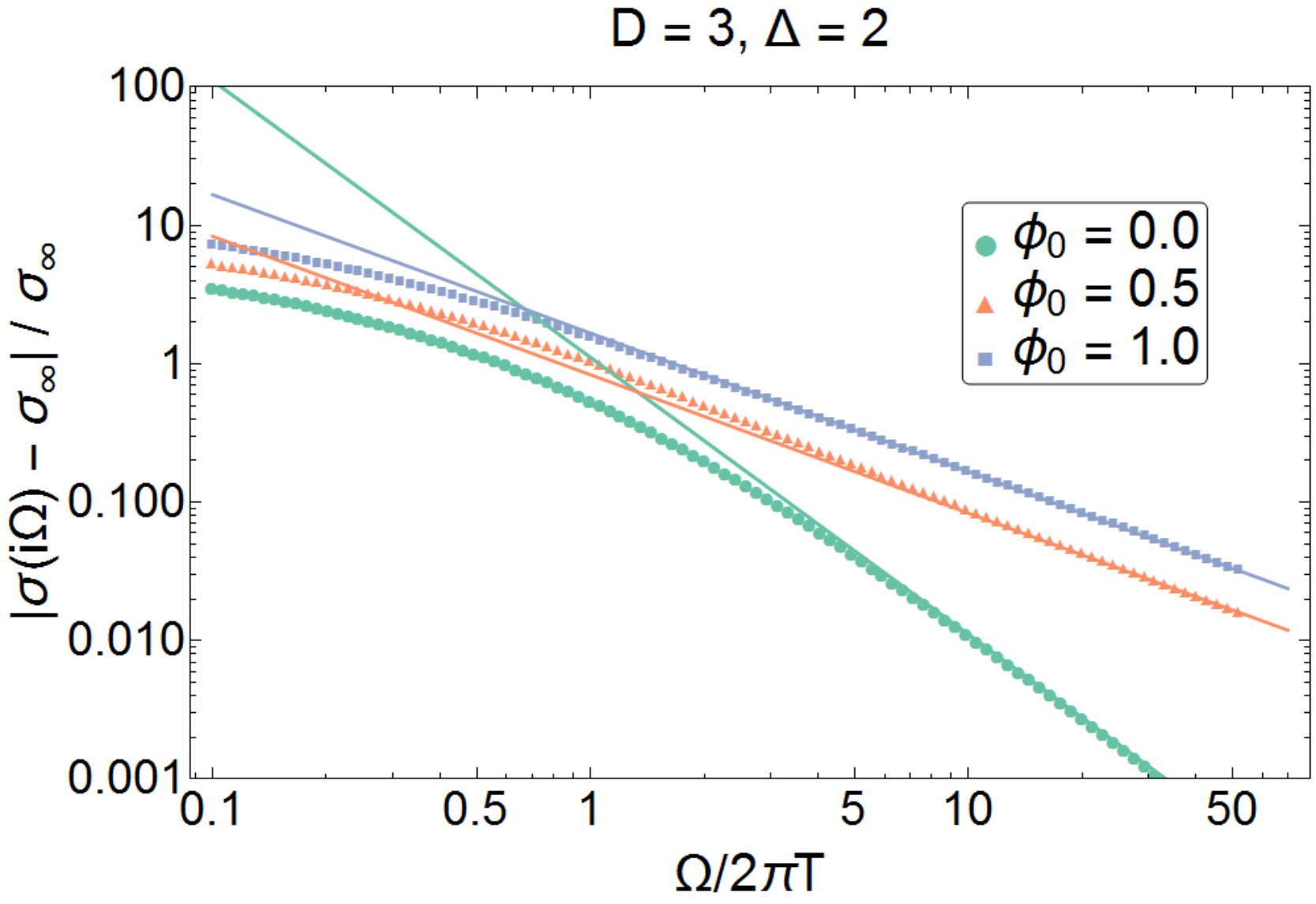
Refer to caption
Figure 7: A comparison of our numerical calculation of σ⁡(i​Ω)\sigma(\mathrm{i}\Omega) (shown in dots) to the first subleading contribution in the asymptotic expansion (3) (shown as thin solid line), when Ω≫T\Omega\gg T. We take Δ=2\Delta=2 and D=3D=3. As predicted in (3), when h=0h=0 the first subleading power Ω−Δ\Omega^{-\Delta} is smaller than when h≠0h\neq 0. For h≠0h\neq 0, the asymptotic corrections are proportional to hh and governed by the same power ΩΔ−D\Omega^{\Delta-D}, leading to a slower decay.

Figure 7 compares the analytic predictions for the asymptotic approach of σ⁡(ω)\sigma(\omega) to its CFT value from Section 4 to our numerical calculation. We find excellent agreement. We observe that the figure numerically confirms that when the scalar deformation is critical (Φ0=0\Phi_{0}=0) the high-frequency conductivity is proportional to ΩD−3−Δ\Omega^{D-3-\Delta}, while when the scalar is tuned away from the critical point (Φ0≠0\Phi_{0}\neq 0) the high-frequency conductivity is proportional to ΩΔ−3\Omega^{\Delta-3}.

5.3.1 Reissner-Nordström Model

So far, the background geometry has been completely thermal. As a consequence, we have not checked the validity of our asymptotic results when ⟨𝒪⟩\langle\mathcal{O}\rangle depends nonlinearly on non-thermal detuning parameters.

To perform such a check, we now consider the real time action

S=∫dD+1​x​−g​(R2​κ2−Z⁡(Φ)​F24​e2−12​(∂Φ)2−V⁡(Φ)),S=\int\mathrm{d}^{D+1}x\sqrt{-g}\left(\frac{R}{2\kappa^{2}}-Z(\Phi)\frac{F^{2}}{4e^{2}}-\frac{1}{2}(\partial\Phi)^{2}-V(\Phi)\right), (137)

with ZZ and VV given in (119). Compared to (46), we have removed the ψ\psi field as well as the Φ​C2\Phi C^{2} coupling. As before, let us imagine that the backreaction of Φ\Phi on the other matter fields can be ignored, but let us now deform the CFT by a finite temperature TT and a finite charge density ρ\rho. The dual geometry to such a theory is known analytically for any density [10], and is called the AdS-Reissner-Nordström black hole:

d​s2=\displaystyle\mathrm{d}s^{2}= L2r+2​u2​(−f⁡(u)​d​t2+δi​j​d​xi​d​xj)+L2​d​u2u2​f​(u)\displaystyle\frac{L^{2}}{r_{+}^{2}u^{2}}\left(-f(u)\mathrm{d}t^{2}+\delta^{ij}\mathrm{d}x_{i}\mathrm{d}x_{j}\right)+\frac{L^{2}\mathrm{d}u^{2}}{u^{2}f(u)} (138a)
A=\displaystyle A= D−1D−2​e​r0​ξκ​L​(1−uD−2)​d​t\displaystyle\sqrt{\frac{D-1}{D-2}}\frac{e\,r_{0}\xi}{\kappa L}(1-u^{D-2})\mathrm{d}t (138b)

where

f⁡(u)=1−(1+ξ2)​uD+ξ2​u2​(D−1)f(u)=1-(1+\xi^{2})u^{D}+\xi^{2}u^{2(D-1)} (139)

and r+r_{+} and ξ\xi are related to the charge density ρ\rho and temperature TT of the black hole:

T\displaystyle T =D−(D−2)​ξ24​π​r+,\displaystyle=\frac{D-(D-2)\xi^{2}}{4\pi r_{+}}, (140a)
ξ2\displaystyle\xi^{2} =κ2​e2​ρ2​r+2​D−2(D−1)​(D−2)​L2​D−4.\displaystyle=\frac{\kappa^{2}e^{2}\rho^{2}r_{+}^{2D-2}}{(D-1)(D-2)L^{2D-4}}. (140b)

The dimensionless radial coordinate uu is once again chosen in such a way that the “outer” black hole horizon is located at u=1u=1 and the asymptotic AdS boundary is located at u→0u\to 0. The black hole horizon is extremal when T=0T=0: this occurs at precisely ξ2=DD−2\xi^{2}=\tfrac{D}{D-2}, and so we will restrict our attention to ξ2<DD−2\xi^{2}<\tfrac{D}{D-2}.

Around this background geometry, we can compute Φ⁡(u)\Phi(u), whose equation of motion is given by

(∇−m2)​Φ−αZ​LD−124​e2​Fa​b​Fa​b=(∇−m2)​Φ+αZ​LD−122​e2​u4​At′2r+2=0.(\nabla-m^{2})\Phi-\frac{\alpha_{Z}L^{\frac{D-1}{2}}}{4e^{2}}F_{ab}F^{ab}=(\nabla-m^{2})\Phi+\frac{\alpha_{Z}L^{\frac{D-1}{2}}}{2e^{2}}\frac{u^{4}A_{t}^{\prime 2}}{r_{+}^{2}}=0. (141)

When ξ≠0\xi\neq 0, we will need to solve this equation numerically to determine Φ⁡(u)\Phi(u).

Due to the presence of the finite charge density, the equations of motion for AxA_{x} become more complicated within linear response [10]. In particular, they couple to fluctuations in the metric components gt​xg_{tx} and gr​xg_{rx}. Using standard techniques, we are able to reduce the equations of motion to a ‘massive’ equation of motion for AxA_{x}:

0=Ax′′+(Z′Z+f′f−D−3u)​Ax′+ω2​r+2f2​Ax−2​(D−1)​(D−2)​u2​ξ2f​Ax.0=A_{x}^{\prime\prime}+\left(\frac{Z^{\prime}}{Z}+\frac{f^{\prime}}{f}-\frac{D-3}{u}\right)A_{x}^{\prime}+\frac{\omega^{2}r_{+}^{2}}{f^{2}}A_{x}-\frac{2(D-1)(D-2)u^{2}\xi^{2}}{f}A_{x}. (142)

This equation is identical to that in [10], up to the dependence on Z⁡(Φ)Z(\Phi), and it can be evaluated numerically. Imposing infalling boundary conditions requires writing Ax​(u)=f​(u)b​F​(u)A_{x}(u)=f(u)^{b}F(u) as before; the boundary condition at the black hole horizon imposing regularity is

F′​(1)F⁡(1)=1(1+2​b)​f′​(1)​(2​(D−1)​(D−2)​ξ2−b​f′​(1)​(Z′​(1)Z⁡(1)+f′′​(1)f′​(1)−D−3u)).\frac{F^{\prime}(1)}{F(1)}=\frac{1}{(1+2b)f^{\prime}(1)}\left(2(D-1)(D-2)\xi^{2}-bf^{\prime}(1)\left(\frac{Z^{\prime}(1)}{Z(1)}+\frac{f^{\prime\prime}(1)}{f^{\prime}(1)}-\frac{D-3}{u}\right)\right)\,. (143)
Refer to caption
Figure 8: Comparison of Re⁡[σ⁡(ω)−σ∞]\mathrm{Re}[\sigma(\omega)-\sigma_{\infty}] between our analytic prediction (3) for the subleading correction to the conductivity, and the full dynamical conductivity at αY​αZ=ξ=1\alpha_{Y}\alpha_{Z}=\xi=1 in D=3D\!=\!3. For simplicity we have set h=0h=0. As in Fig. 7, we observe excellent agreement when ω≫T\omega\gg T; at low frequency, the structure of σ⁡(ω)\sigma(\omega) is highly non-trivial in this background: see Figure 9.

Figure 8 demonstrates agreement between our analytic prediction (3) for the high frequency corrections to σ⁡(ω)\sigma(\omega), and a full numerical computation. It is important to keep in mind that in this more generic geometry, the conductivity is not given by the CFT result even when h=T=0h=T=0. Indeed, due to the presence of a finite charge density ρ\rho, and hence chemical potential μ\mu, the conductivity takes the following form:

σ⁡(ω)=σ∞⋅(i​ω)D−3​[1+𝒜​h(i​ω)D−Δ+ℬ​⟨𝒪⟩(i​ω)Δ−𝒜′​μ2ω2+⋯].\sigma(\omega)=\sigma_{\infty}\cdot(\mathrm{i}\omega)^{D-3}\left[1+\mathcal{A}\frac{h}{(\mathrm{i}\omega)^{D-\Delta}}+\mathcal{B}\frac{\langle\mathcal{O}\rangle}{(\mathrm{i}\omega)^{\Delta}}-\mathcal{A}^{\prime}\frac{\mu^{2}}{\omega^{2}}+\cdots\right]. (144)

The coefficients 𝒜\mathcal{A} and ℬ\mathcal{B} are given in (36) and (110). The coefficient 𝒜′\mathcal{A}^{\prime} is related to the four-point correlation function ⟨J​J​J​J⟩\langle JJJJ\rangle in the CFT, which is non-vanishing in our holographic model due to graviton exchange in the bulk. The 𝒜′\mathcal{A}^{\prime} term is in fact the counterpart of the higher order correction (h/ωD−Δ)2(h/\omega^{D-\Delta})^{2}, where the role of 𝒪\mathcal{O} is played by the charge density JtJ_{t}, and the chemical potential μ\mu plays the role of hh. In (144), we see that if h=0h=0, it is necessary to deform this field theory at finite charge density by a relevant operator of dimension Δ<2\Delta<2 in order for the expansion (3) to hold.

Refer to caption
Figure 9: The real part of the conductivity for D=3D=3, Δ=2\Delta=2 and ‘charge parameter’ ξ=1\xi=1 for various values of αZ​αW\alpha_{Z}\alpha_{W}. Coupling to the relevant operator 𝒪\mathcal{O} leads to pronounced features in Re⁡(σ)\mathrm{Re}(\sigma) at intermediate frequencies, in addition to modifying the high frequency asymptotics as in (144).

In Figure 9 we plot Re⁡(σ⁡(ω))\mathrm{Re}(\sigma(\omega)) as a function of αW​αZ\alpha_{W}\alpha_{Z}, corresponding to increasing 𝒞J​J​𝒪\mathcal{C}_{JJ\mathcal{O}}. Unlike before, in this field theory at finite charge density we observe non-trivial structure even when αW​αZ=0\alpha_{W}\alpha_{Z}=0, when the scalar operator 𝒪\mathcal{O} is decoupled. This is a consequence of the fact that finite μ\mu already corresponds to a non-trivial deformation of the CFT. Upon setting αW​αZ>0\alpha_{W}\alpha_{Z}>0, we observe additional structure emerge in Figure 9, associated with the coupling to the operator 𝒪\mathcal{O}.

In Figure 9, one may notice the presence of “missing” spectral weight. This spectral weight has in fact shifted into a δ\delta-function at ω=0\omega=0: ‘hydrodynamics’ constrains the low frequency conductivity to be [10]

σ⁡(ω→0)=ρ2ϵ+P​(π​δ​(ω)+iω)+⋯.\sigma(\omega\rightarrow 0)=\frac{\rho^{2}}{\epsilon+P}\left(\pi\delta(\omega)+\frac{\mathrm{i}}{\omega}\right)+\cdots. (145)

Here ϵ\epsilon is the energy density and PP is the pressure. A uniform and static electric field can impart momentum into a system at finite charge density at a fixed rate via the Lorentz force: this is the origin of this δ\delta function. This δ\delta function must be taken into account when evaluating sum rules, and upon doing so, the sum rules for the conductivity are restored.

6 Lifshitz Holography

In this section, we will now extend our analysis to holographic quantum critical systems with dynamic critical exponent z≠1z\neq 1. This means that there is an emergent scale invariance of the low energy effective theory, but time and space scale separately. Under a rescaling λ\lambda:

𝐱→λ​𝐱,t→λz​t.\mathbf{x}\rightarrow\lambda\mathbf{x},\;\;\;\;t\rightarrow\lambda^{z}t. (146)

Because time and space are no longer related through Lorentz transformations, in this section we will not talk about the spacetime dimension DD, but instead the spatial dimension d=D−1d=D-1, as is more conventional in condensed matter.

As argued in [20], the high frequency behavior of correlation functions in such Lifshitz theories will share many features with CFTs. For simplicity, we will only talk about the conductivity in this section. In particular, the asymptotic expansion of the conductivity will be modified from (3) to

σ⁡(i​Ω)=Ωd−2z​[𝒞J​J+𝒜​hΩ1+d−Δz+ℬ​⟨𝒪⟩ΩΔz+⋯].\sigma(\mathrm{i}\Omega)=\Omega^{\frac{d-2}{z}}\left[\mathcal{C}_{JJ}+\frac{\mathcal{A}h}{\Omega^{1+\frac{d-\Delta}{z}}}+\frac{\mathcal{B}\langle\mathcal{O}\rangle}{\Omega^{\frac{\Delta}{z}}}+\cdots\right]. (147)

We now present a holographic Lifshitz theory where this result can be shown explicitly, and a relationship between 𝒜\mathcal{A} and ℬ\mathcal{B} can be obtained.

6.1 Bulk Model

We first begin by outlining the holographic model which we study. The bulk action is given by

S=Sbg​[gμ​ν,Φ]+∫dd+2​x​−g​Z⁡(Φ)4​e2​Fa​b​Fa​b,S=S_{\mathrm{bg}}[g_{\mu\nu},\Phi]+\int\mathrm{d}^{d+2}x\sqrt{-g}\frac{Z(\Phi)}{4e^{2}}F_{ab}F^{ab}, (148)

with SbgS_{\mathrm{bg}} the action for the metric and the other bulk fields which support the Lifshitz geometry, and the remaining term describing a fluctuating gauge field. We take Z⁡(Φ)Z(\Phi) to be given by (47b), as before. Specific forms of SbgS_{\mathrm{bg}} can be found in [36], for example, but they will not be relevant for our purpose. We will take our background to be uncharged under Fa​bF_{ab}, the bulk field under which we will compute the conductivity. The quadratic terms in Φ\Phi in SbgS_{\mathrm{bg}} are given by

Sbg=∫dd+2​x​−g​(12​(∂Φ)2+Δ⁡(Δ−d−z)L2​Φ2)+⋯.S_{\mathrm{bg}}=\int\mathrm{d}^{d+2}x\sqrt{-g}\left(\frac{1}{2}(\partial\Phi)^{2}+\frac{\Delta(\Delta-d-z)}{L^{2}}\Phi^{2}\right)+\cdots. (149)

Note that the mass of Φ2\Phi^{2} is distinct from that in (47d), once z≠1z\neq 1.

The background metric of the Lifshitz theory is given by [36]

d​s2=L2r2​[d​r2−d​t2r2​(z−1)+d​𝐱2].\mathrm{d}s^{2}=\frac{L^{2}}{r^{2}}\left[\mathrm{d}r^{2}-\frac{\mathrm{d}t^{2}}{r^{2(z-1)}}+\mathrm{d}\mathbf{x}^{2}\right]. (150)

The isometries of this metric map on to the Lifshitz symmetries of the dual field theory, and as a consequence the correlation functions of the dual theory are necessarily Lifshitz invariant. As Lifshitz invariance is a much weaker requirement than conformal invariance [37, 38, 39], it is not clear that holographic models can capture the dynamics of generic Lifshitz theories. Nonetheless, we will be able to demonstrate a generalization of (3) in at least one class of interacting Lifshitz theories, and although our specific results for 𝒜\mathcal{A} and ℬ\mathcal{B} are not generic, we expect that the qualitative features of this model are more robust. One can also study more complicated bulk models than (148), as the symmetries of Lifshitz theories are far less constraining [40].

In order to compute the conductivity, we must note changes to the holographic dictionary in a Lifshitz background. Following the discussion of holographic renormalization in [10], one finds:

Φ\displaystyle\Phi =hLd/2​rd+z−Δ+⟨𝒪⟩(2​Δ−d−z)​Ld/2​rΔ+⋯,\displaystyle=\frac{h}{L^{d/2}}r^{d+z-\Delta}+\frac{\langle\mathcal{O}\rangle}{(2\Delta-d-z)L^{d/2}}r^{\Delta}+\cdots, (151a)
Ax\displaystyle A_{x} =Ax0+e2Ld−2​⟨Jx⟩d+z−2​rd+z−2+⋯.\displaystyle=A_{x}^{0}+\frac{e^{2}}{L^{d-2}}\frac{\langle J_{x}\rangle}{d+z-2}r^{d+z-2}+\cdots. (151b)

6.2 Asymptotics of the Conductivity

The equations of motion for the gauge field in the background (150) are

0=1g​∂a(Z​g​Fa​x)=rd+z+1​∂r(Z⁡(Φ⁡(r))​r1−d−z​∂rAx)−Ω2​Z​(Φ⁡(r))​r2​z​Ax.0=\frac{1}{\sqrt{g}}\partial_{a}\left(Z\sqrt{g}F^{ax}\right)=r^{d+z+1}\partial_{r}\left(Z(\Phi(r))r^{1-d-z}\partial_{r}A_{x}\right)-\Omega^{2}Z(\Phi(r))r^{2z}A_{x}. (152)

Let us now define the variable

R≡Ωz​rz.R\equiv\frac{\Omega}{z}r^{z}. (153)

By the same logic as before, the limit Ω→∞\Omega\rightarrow\infty becomes completely regular, with (152) becoming

0=Rd−2z​∂R(Z⁡((z​RΩ)1/z)​R−d−2z​∂RAx)−Z⁡((z​RΩ)1/z)​Ax0=R^{\frac{d-2}{z}}\partial_{R}\left(Z\left(\left(\frac{zR}{\Omega}\right)^{1/z}\right)R^{-\frac{d-2}{z}}\partial_{R}A_{x}\right)-Z\left(\left(\frac{zR}{\Omega}\right)^{1/z}\right)A_{x} (154)

At Ω=∞\Omega=\infty, the solution to this equation with the correct boundary conditions is

Ax=K^d+z−22​z​(R)𝒵⁡(d+z−22​z).A_{x}=\frac{\hat{\mathrm{K}}_{\frac{d+z-2}{2z}}\left(R\right)}{\mathcal{Z}\left(\frac{d+z-2}{2z}\right)}. (155)

At finite Ω\Omega, we must solve

∂R2Ax−d−2z​R​∂RAx−Ax\displaystyle\partial_{R}^{2}A_{x}-\frac{d-2}{zR}\partial_{R}A_{x}-A_{x} =𝔞⁡(R)​Ax−Rd−2z​∂R(𝔞⁡(R)​R−d−2z​∂RAx)\displaystyle=\mathfrak{a}(R)A_{x}-R^{\frac{d-2}{z}}\partial_{R}\left(\mathfrak{a}(R)R^{-\frac{d-2}{z}}\partial_{R}A_{x}\right) (156)

perturbatively in 𝔞⁡(R)\mathfrak{a}(R). This is exactly analogous to the solution of (100). Following (108), and using that

𝔞⁡(R)=αZ​h​(z​RΩ)d+z−Δz+αZ​⟨𝒪⟩2​Δ−d−z​(z​RΩ)Δz,\mathfrak{a}(R)=\alpha_{Z}h\left(\frac{zR}{\Omega}\right)^{\frac{d+z-\Delta}{z}}+\frac{\alpha_{Z}\langle\mathcal{O}\rangle}{2\Delta-d-z}\left(\frac{zR}{\Omega}\right)^{\frac{\Delta}{z}}, (157)

we obtain (analogously to (109)):

Ax​(R→0)\displaystyle A_{x}(R\rightarrow 0) ≈K^d+z−22​z​(R)𝒵⁡(d+z−22​z)+Rd+z−2zd+z−2z×\displaystyle\approx\frac{\hat{\mathrm{K}}_{\frac{d+z-2}{2z}}\left(R\right)}{\mathcal{Z}\left(\frac{d+z-2}{2z}\right)}+\frac{R^{\frac{d+z-2}{z}}}{\frac{d+z-2}{z}}\times
{αZh(zΩ)d+z−Δz(d+z−Δ)​(Δ−2)2​z2​𝒵​(d+z−22)2Ψ(d+z−Δz,d+z−22​z)\displaystyle\left\{\alpha_{Z}h\left(\frac{z}{\Omega}\right)^{\frac{d+z-\Delta}{z}}\frac{(d+z-\Delta)(\Delta-2)}{2z^{2}\mathcal{Z}(\frac{d+z-2}{2})^{2}}\Psi\left(\frac{d+z-\Delta}{z},\frac{d+z-2}{2z}\right)\right.
+αZ​⟨𝒪⟩2​Δ−d−z(zΩ)ΔzΔ⁡(d+z−Δ−2)2​z2​𝒵​(d+z−22​z)2Ψ(Δz,d+z−22​z)}.\displaystyle\left.+\frac{\alpha_{Z}\langle\mathcal{O}\rangle}{2\Delta-d-z}\left(\frac{z}{\Omega}\right)^{\frac{\Delta}{z}}\frac{\Delta(d+z-\Delta-2)}{2z^{2}\mathcal{Z}(\frac{d+z-2}{2z})^{2}}\Psi\left(\frac{\Delta}{z},\frac{d+z-2}{2z}\right)\right\}. (158)

Hence, the conductivity is

σ⁡(i​Ω)\displaystyle\sigma(\mathrm{i}\Omega) =Ld−2e2Ωd−2z[𝒞J​J+αZ​z2−z−Δz​(d+z−Δ)​(Δ−2)2​𝒵​(d+z−22​z)2Ψ(d+z−Δz,d+z−22​z)hΩd+z−Δz\displaystyle=\frac{L^{d-2}}{e^{2}}\Omega^{\frac{d-2}{z}}\left[\mathcal{C}_{JJ}+\frac{\alpha_{Z}z^{\frac{2-z-\Delta}{z}}(d+z-\Delta)(\Delta-2)}{2\mathcal{Z}(\frac{d+z-2}{2z})^{2}}\Psi\left(\frac{d+z-\Delta}{z},\frac{d+z-2}{2z}\right)\frac{h}{\Omega^{\frac{d+z-\Delta}{z}}}\right.
+αZ​z2−d−2​z+Δz​Δ​(d+z−Δ−2)2​(2​Δ−d−z)​𝒵​(d+z−22​z)2Ψ(Δz,d+z−22​z)⟨𝒪⟩ΩΔz].\displaystyle\left.+\frac{\alpha_{Z}z^{\frac{2-d-2z+\Delta}{z}}\Delta(d+z-\Delta-2)}{2(2\Delta-d-z)\mathcal{Z}(\frac{d+z-2}{2z})^{2}}\Psi\left(\frac{\Delta}{z},\frac{d+z-2}{2z}\right)\frac{\langle\mathcal{O}\rangle}{\Omega^{\frac{\Delta}{z}}}\right]. (159)

6.3 Three-Point Function and (Holographic) Lifshitz Perturbation Theory

Now, we follow the construction of Section 3.1.3 and compare our holographic result to “Lifshitz perturbation theory”.

The properly normalized solution to the scalar equation of motion in a Lifshitz background that follows from (149),

Δ⁡(Δ−d−z)L2​Φ=∇a∇a​Φ,\frac{\Delta(\Delta-d-z)}{L^{2}}\Phi=\nabla_{a}\nabla^{a}\Phi, (160)

is

Φ⁡(p3,r)=ei​p3⋅x​rd+z−Δ​K^2​Δ−d−z2​z​(ωz​rz)𝒵⁡(2​Δ−d−z2​z)​Ld/2​j𝒪​(p3).\Phi(p_{3},r)=\mathrm{e}^{\mathrm{i}p_{3}\cdot x}r^{d+z-\Delta}\frac{\hat{\mathrm{K}}_{\frac{2\Delta-d-z}{2z}}(\frac{\omega}{z}r^{z})}{\mathcal{Z}(\frac{2\Delta-d-z}{2z})L^{d/2}}j_{\mathcal{O}}(p_{3}). (161)

The cubic contribution to the bulk action becomes

Sbulk\displaystyle S_{\mathrm{bulk}} =∫dd+2​x​g​αZ​Ld/2​Φ​(p3)e2​ga​b​gx​x​∂aAx​(p1)​∂bAx​(p2)\displaystyle=\int\mathrm{d}^{d+2}x\sqrt{g}\frac{\alpha_{Z}L^{d/2}\Phi(p_{3})}{e^{2}}g^{ab}g^{xx}\partial_{a}A_{x}(p_{1})\partial_{b}A_{x}(p_{2})
=−∫dd+2xAx(p1)∂a[gαZ​Ld/2​Φ​(p3)e2ga​bgx​x∂bAx(p2)]\displaystyle=-\int\mathrm{d}^{d+2}xA_{x}(p_{1})\partial_{a}\left[\sqrt{g}\frac{\alpha_{Z}L^{d/2}\Phi(p_{3})}{e^{2}}g^{ab}g^{xx}\partial_{b}A_{x}(p_{2})\right]
=−∫dd+2xAx(p1)gαZ​Ld/2e2ga​bgx​x∂bAx(p2)∂aΦ(p3)\displaystyle=-\int\mathrm{d}^{d+2}xA_{x}(p_{1})\sqrt{g}\frac{\alpha_{Z}L^{d/2}}{e^{2}}g^{ab}g^{xx}\partial_{b}A_{x}(p_{2})\partial_{a}\Phi(p_{3})
=αZ​Ld/22​e2​∫dd+2​x​g​Ax​(p1)​Ax​(p2)​[gx​x​Δ⁡(Δ−d−z)L2​Φ​(p3)+2r​gx​x​gr​r​∂rΦ⁡(p3)].\displaystyle=\frac{\alpha_{Z}L^{d/2}}{2e^{2}}\int\mathrm{d}^{d+2}x\sqrt{g}A_{x}(p_{1})A_{x}(p_{2})\left[g^{xx}\frac{\Delta(\Delta-d-z)}{L^{2}}\Phi(p_{3})+\frac{2}{r}g^{xx}g^{rr}\partial_{r}\Phi(p_{3})\right]. (162)

Using (155) and (161), along with (69) we obtain (suppressing the δ\delta-function for momenta, and the integrals in the boundary directions)

Sbulk\displaystyle S_{\mathrm{bulk}} =αZ​Ld−22​e2∫d​rrd+z−1K^d+z−22​z​(p1z​rz)𝒵⁡(d+z−22​z)K^d+z−22​z​(p2z​rz)𝒵⁡(d+z−22​z)[Δ(Δ−d−z)K^2​Δ−d−z2​z​(p3z​rz)𝒵⁡(2​Δ−d−z2​z)\displaystyle=\frac{\alpha_{Z}L^{d-2}}{2e^{2}}\int\frac{\mathrm{d}r}{r^{d+z-1}}\frac{\hat{\mathrm{K}}_{\frac{d+z-2}{2z}}\left(\frac{p_{1}}{z}r^{z}\right)}{\mathcal{Z}\left(\frac{d+z-2}{2z}\right)}\frac{\hat{\mathrm{K}}_{\frac{d+z-2}{2z}}\left(\frac{p_{2}}{z}r^{z}\right)}{\mathcal{Z}\left(\frac{d+z-2}{2z}\right)}\left[\Delta(\Delta-d-z)\frac{\hat{\mathrm{K}}_{\frac{2\Delta-d-z}{2z}}(\frac{p_{3}}{z}r^{z})}{\mathcal{Z}(\frac{2\Delta-d-z}{2z})}\right.
+2​Δ​K^2​Δ−d−z2​z​(p3z​rz)𝒵⁡(2​Δ−d−z2​z)−2​z​K^2​Δ−d+z2​z​(p3z​rz)𝒵⁡(2​Δ−d−z2​z)]rd+z−Δ\displaystyle\left.+\frac{2\Delta\hat{\mathrm{K}}_{\frac{2\Delta-d-z}{2z}}(\frac{p_{3}}{z}r^{z})}{\mathcal{Z}(\frac{2\Delta-d-z}{2z})}-\frac{2z\hat{\mathrm{K}}_{\frac{2\Delta-d+z}{2z}}(\frac{p_{3}}{z}r^{z})}{\mathcal{Z}(\frac{2\Delta-d-z}{2z})}\right]r^{d+z-\Delta} (163)

Changing variables to ρ=rz/z\rho=r^{z}/z, we obtain

Sbulk\displaystyle S_{\mathrm{bulk}} =αZ​Ld−22​e2∫d​ρ​(z​ρ)2−z−Δz𝒵​(d+z−22​z)2​𝒵​(2​Δ−d−z2​z)[Δ(Δ+2−d−z)K^2​Δ−d−z2​z(p3ρ)\displaystyle=\frac{\alpha_{Z}L^{d-2}}{2e^{2}}\int\frac{\mathrm{d}\rho(z\rho)^{\frac{2-z-\Delta}{z}}}{\mathcal{Z}(\frac{d+z-2}{2z})^{2}\mathcal{Z}(\frac{2\Delta-d-z}{2z})}\left[\Delta(\Delta+2-d-z)\hat{\mathrm{K}}_{\frac{2\Delta-d-z}{2z}}(p_{3}\rho)\right.
−2zK^2​Δ−d+z2​z(p3ρ)]K^d+z−22​z(p1ρ)K^d+z−22​z(p2ρ).\displaystyle\left.-2z\hat{\mathrm{K}}_{\frac{2\Delta-d+z}{2z}}(p_{3}\rho)\right]\hat{\mathrm{K}}_{\frac{d+z-2}{2z}}(p_{1}\rho)\hat{\mathrm{K}}_{\frac{d+z-2}{2z}}(p_{2}\rho). (164)

Analogously to (72), we obtain

⟨Jx​(Ω1)​Jx​(Ω2)​𝒪​(Ω3)⟩0\displaystyle\langle J_{x}(\Omega_{1})J_{x}(\Omega_{2})\mathcal{O}(\Omega_{3})\rangle_{0}
=\displaystyle= αZ​Ld−2​z2−z−Δze2​𝒵​(d+z−22​z)2​𝒵​(2​Δ−d−z2​z){zI(d+z2​z,d+z−22​z,d+z−22​z,2​Δ−d+z2​z)\displaystyle\frac{\alpha_{Z}L^{d-2}z^{\frac{2-z-\Delta}{z}}}{e^{2}\mathcal{Z}(\frac{d+z-2}{2z})^{2}\mathcal{Z}(\frac{2\Delta-d-z}{2z})}\left\{zI\left(\frac{d+z}{2z},\frac{d+z-2}{2z},\frac{d+z-2}{2z},\frac{2\Delta-d+z}{2z}\right)\right.
−Δ2(Δ+2−d−z)I(d−z2​z,d+z−22​z,d+z−22​z,2​Δ−d−z2​z)}.\displaystyle\left.-\frac{\Delta}{2}(\Delta+2-d-z)I\left(\frac{d-z}{2z},\frac{d+z-2}{2z},\frac{d+z-2}{2z},\frac{2\Delta-d-z}{2z}\right)\right\}. (165)

We now attempt to follow the arguments of conformal perturbation theory. We expect to find that the conductivity takes an analogous form to (3):

σ⁡(i​Ω)=Ωd−2z​[σ∞+𝒜​hΩd+z−Δz+ℬ​⟨𝒪⟩Ωd+z−Δz],\sigma(\mathrm{i}\Omega)=\Omega^{\frac{d-2}{z}}\left[\sigma_{\infty}+\frac{\mathcal{A}h}{\Omega^{\frac{d+z-\Delta}{z}}}+\frac{\mathcal{B}\langle\mathcal{O}\rangle}{\Omega^{\frac{d+z-\Delta}{z}}}\right], (166)

and now use the form of the three-point correlator (165) to fix 𝒜\mathcal{A} and ℬ\mathcal{B}. We take p1,2,3p_{1,2,3} to be given by (11), and Taylor expand in p/Ωp/\Omega. We find a regular term as p→0p\rightarrow 0, given by

⟨Jx(Ω)\displaystyle\langle J_{x}(\Omega) Jx(−Ω)𝒪(0)⟩0=αZ​Ld−2​z2−z−Δz​ΩΔ−z−2ze2​𝒵​(d+z−22​z)2​𝒵​(2​Δ−d−z2​z){z𝒵(2​Δ−d+z2​z)\displaystyle J_{x}(-\Omega)\mathcal{O}(0)\rangle_{0}=\frac{\alpha_{Z}L^{d-2}z^{\frac{2-z-\Delta}{z}}\Omega^{\frac{\Delta-z-2}{z}}}{e^{2}\mathcal{Z}(\frac{d+z-2}{2z})^{2}\mathcal{Z}(\frac{2\Delta-d-z}{2z})}\left\{z\mathcal{Z}\left(\frac{2\Delta-d+z}{2z}\right)\right.
−Δ2(Δ+2−d−z)𝒵(2​Δ−d−z2​z)}Ψ(d+z−Δz,d+z−22​z)\displaystyle\left.-\frac{\Delta}{2}(\Delta+2-d-z)\mathcal{Z}\left(\frac{2\Delta-d-z}{2z}\right)\right\}\Psi\left(\frac{d+z-\Delta}{z},\frac{d+z-2}{2z}\right)
=−αZ​Ld−2​z2−z−Δz​ΩΔ−z−2ze2​𝒵​(d+z−22​z)2​(1−Δ2)​(d+z−Δ)​Ψ​(d+z−Δz,d+z−22​z).\displaystyle=-\frac{\alpha_{Z}L^{d-2}z^{\frac{2-z-\Delta}{z}}\Omega^{\frac{\Delta-z-2}{z}}}{e^{2}\mathcal{Z}(\frac{d+z-2}{2z})^{2}}\left(1-\frac{\Delta}{2}\right)(d+z-\Delta)\Psi\left(\frac{d+z-\Delta}{z},\frac{d+z-2}{2z}\right). (167)

Similarly, we find a non-analytic contribution in pp:

⟨Jx(Ω)\displaystyle\langle J_{x}(\Omega) Jx(−Ω)𝒪(p)⟩0=⋯−αZ​Ld−2​z2−z−Δz​ΩΔ−z−2ze2​𝒵​(d+z−22​z)2​𝒵​(2​Δ−d−z2​z)×\displaystyle J_{x}(-\Omega)\mathcal{O}(p)\rangle_{0}=\cdots-\frac{\alpha_{Z}L^{d-2}z^{\frac{2-z-\Delta}{z}}\Omega^{\frac{\Delta-z-2}{z}}}{e^{2}\mathcal{Z}(\frac{d+z-2}{2z})^{2}\mathcal{Z}(\frac{2\Delta-d-z}{2z})}\times
Δ⁡(Δ+2−d−z)2​𝒵​(d+z−2​Δ2​z)​Ψ​(Δz,d+z−22​z)​(pΩ)2​Δ−d−zz.\displaystyle\frac{\Delta(\Delta+2-d-z)}{2}\mathcal{Z}\left(\frac{d+z-2\Delta}{2z}\right)\Psi\left(\frac{\Delta}{z},\frac{d+z-2}{2z}\right)\left(\frac{p}{\Omega}\right)^{\frac{2\Delta-d-z}{z}}. (168)

Following the logic of conformal perturbation theory, we fix

𝒜\displaystyle\mathcal{A} =−αZ​Ld−2​z2−z−Δze2​𝒵​(d+z−22​z)2​(1−Δ2)​(d+z−Δ)​Ψ​(d+z−Δz,d+z−22​z),\displaystyle=-\frac{\alpha_{Z}L^{d-2}z^{\frac{2-z-\Delta}{z}}}{e^{2}\mathcal{Z}(\frac{d+z-2}{2z})^{2}}\left(1-\tfrac{\Delta}{2}\right)(d+z-\Delta)\Psi\left(\frac{d+z-\Delta}{z},\frac{d+z-2}{2z}\right), (169a)
ℬ\displaystyle\mathcal{B} =−αZ​Ld−2​z2−z−Δz𝒞𝒪​𝒪​e2​𝒵​(d+z−22​z)2​𝒵​(2​Δ−d−z2​z)\displaystyle=-\frac{\alpha_{Z}L^{d-2}z^{\frac{2-z-\Delta}{z}}}{\mathcal{C}_{\mathcal{OO}}e^{2}\mathcal{Z}(\frac{d+z-2}{2z})^{2}\mathcal{Z}(\frac{2\Delta-d-z}{2z})}
×Δ⁡(Δ+2−d−z)2​𝒵​(d+z−2​Δ2​z)​Ψ​(Δz,d+z−22​z).\displaystyle\;\;\;\;\;\;\;\;\;\;\;\;\;\times\frac{\Delta(\Delta+2-d-z)}{2}\mathcal{Z}\left(\frac{d+z-2\Delta}{2z}\right)\Psi\left(\frac{\Delta}{z},\frac{d+z-2}{2z}\right). (169b)

The computation of 𝒞𝒪​𝒪\mathcal{C}_{\mathcal{OO}} in a holographic Lifshitz theory proceeds along the lines of Section 3.1.1. Employing (151) and (161) we find

𝒞𝒪​𝒪=2​Δ−d−zz2​Δ−d−zz​𝒵⁡(d+z−2​Δ2​z)𝒵⁡(2​Δ−d−z2​z).\mathcal{C}_{\mathcal{OO}}=\frac{2\Delta-d-z}{z^{\frac{2\Delta-d-z}{z}}}\frac{\mathcal{Z}(\frac{d+z-2\Delta}{2z})}{\mathcal{Z}(\frac{2\Delta-d-z}{2z})}. (170)

Plugging this result into (169), we see complete agreement with (159).

7 Sum Rules

One of the main applications of the high frequency asymptotics that we have been discussing is the derivation of sum rules for dynamical response functions. The most familiar sum rules are associated with the conductivity σ⁡(ω)\sigma(\omega). Such conductivity sum rules in near-critical systems were shown recently in [20], and we review the arguments here, and generalize them to other response functions. Our first goal is to understand when the following identity holds:

∫0∞d​ω​Re​(σ⁡(ω,T,h)−𝒞J​J⋅(i​ω)d−2z)=0,\int\limits_{0}^{\infty}\mathrm{d}\omega\;\mathrm{Re}\left(\sigma(\omega;T,h)-\mathcal{C}_{JJ}\cdot(\mathrm{i}\omega)^{\frac{d-2}{z}}\right)=0, (171)

where dd is the number of spatial dimensions. This is a highly non-trivial constraint on the conductivity, which is a scaling function of 2 variables: ω/T\omega/T and h/Th/T. At z=1z=1, (171) was derived under certain conditions for CFTs, which we review below [8, 20, 13, 41]. We will also analyze its validity for Lifshitz theories z≠1z\neq 1.

The asymptotic expansion (147) allows us to understand precisely when (171) will hold. We need the first subleading term in an asymptotic expansion of σ⁡(ω)\sigma(\omega) to decay faster than ω−1\omega^{-1} as ω→∞\omega\rightarrow\infty. If this is the case, then we may evaluate the integral of (171) via contour integration, choosing a semicircular contour in the upper half plane and using analyticity of σ⁡(ω)\sigma(\omega) to show that no poles or branch cuts may be enclosed by the contour (see e.g. [11, 8, 20]). From (147), we conclude that the sum rule is valid when

d+z−2<Δ<2,d+z-2<\Delta<2, (172)

a result first shown in [20]. The first inequality (the lower bound on Δ\Delta) comes from demanding that the 𝒜\mathcal{A} term decay faster than ω−1\omega^{-1}; the second inequality (the upper bound on Δ\Delta) comes from demanding the same of the ℬ\mathcal{B} term. Hence, exactly at the critical point (h=0h=0), we find the somewhat weaker bound that Δ>d−2+z\Delta>d-2+z, which agrees with the result for d=2d=2 CFTs [8], i.e. Δ>1\Delta>1.

For general dd and zz, the analogue of (171) for the scalar 2-point function ⟨𝒪0​𝒪0⟩\langle\mathcal{O}_{0}\mathcal{O}_{0}\rangle is

∫0∞d​ω​Im​(⟨𝒪0​(ω)​𝒪0​(−ω)⟩ω−𝒞𝒪0​𝒪0​(i​ω)2​Δ0−d−zzω)=0.\int\limits_{0}^{\infty}\mathrm{d}\omega\;\mathrm{Im}\left(\frac{\langle\mathcal{O}_{0}(\omega)\mathcal{O}_{0}(-\omega)\rangle}{\omega}-\mathcal{C}_{\mathcal{O}_{0}\mathcal{O}_{0}}\frac{(\mathrm{i}\omega)^{\frac{2\Delta_{0}-d-z}{z}}}{\omega}\right)=0. (173)

where Im⁡(⟨𝒪0​(ω)​𝒪0​(−ω)⟩)\mathrm{Im}(\langle\mathcal{O}_{0}(\omega)\mathcal{O}_{0}(-\omega)\rangle) is the usual spectral function. The generalization of (3) to z≠1z\neq 1 is

⟨𝒪0​(ω)​𝒪0​(−ω)⟩=(i​ω)2​Δ0−d−zz​[𝒞𝒪0​𝒪0+𝒜​h(i​ω)1+d−Δz+ℬ​⟨𝒪⟩(i​ω)Δz+⋯].\langle\mathcal{O}_{0}(\omega)\mathcal{O}_{0}(-\omega)\rangle=(\mathrm{i}\omega)^{\frac{2\Delta_{0}-d-z}{z}}\left[\mathcal{C}_{\mathcal{O}_{0}\mathcal{O}_{0}}+\frac{\mathcal{A}h}{(\mathrm{i}\omega)^{1+\frac{d-\Delta}{z}}}+\frac{\mathcal{B}\langle\mathcal{O}\rangle}{(\mathrm{i}\omega)^{\frac{\Delta}{z}}}+\cdots\right]. (174)

In this paper, we have demonstrated this asymptotic expansion carefully for CFTs (with z=1z=1), but we expect that it also holds true for a large class of systems with z≠1z\neq 1 (including the Lifshitz holographic models described above). If 2​Δ0>d+z2\Delta_{0}>d+z, then the subtraction in (173) is not badly behaved near ω=0\omega=0, where we expect that at any finite TT or hh, any divergences in ⟨𝒪0​𝒪0⟩\langle\mathcal{O}_{0}\mathcal{O}_{0}\rangle will be resolved. From (174), we conclude that (173) holds so long as

2​Δ0−d−z<Δ<2​(d+z−Δ0),2\Delta_{0}-d-z<\Delta<2(d+z-\Delta_{0}), (175)

using similar logic to the previous paragraph. As with the conductivity, the upper bound on Δ\Delta is only needed if h≠0h\neq 0. We note that (172) is a special case of (175), when Δ0=d+z−1\Delta_{0}=d+z-1, consistent with the fact that in a Lifshitz theory the operator dimension of JxJ_{x} is d+z−1d+z-1 (measured in units of inverse length).

We now turn to sum rules for the shear viscosity. These were studied in certain critical phases (CFTs without a relevant singlet 𝒪\mathcal{O}) in [11, 12, 13]. Here we generalize to quantum critical points with general zz, and also to theories detuned by a relevant operator 𝒪\mathcal{O}. We expect the asymptotic form of the viscosity to be

η⁡(ω)=(i​ω)dz​[𝒞T​T+𝒜​h(i​ω)1+d−Δz+ℬ​⟨𝒪⟩(i​ω)Δz+ℬT​P(i​ω)1+dz+⋯].\eta(\omega)=(\mathrm{i}\omega)^{\frac{d}{z}}\left[\mathcal{C}_{TT}+\frac{\mathcal{A}h}{(\mathrm{i}\omega)^{1+\frac{d-\Delta}{z}}}+\frac{\mathcal{B}\langle\mathcal{O}\rangle}{(\mathrm{i}\omega)^{\frac{\Delta}{z}}}+\frac{\mathcal{B}_{T}P}{(\mathrm{i}\omega)^{1+\frac{d}{z}}}+\cdots\right]. (176)

for generic dd and zz. As we will shortly see, it is important to keep track of a term proportional to the pressure P=⟨Tx​x⟩P=\langle T_{xx}\rangle in the asymptotic expansion. Such a term can arise due to the stress tensor appearing in the OPE of Tx​y​Tx​yT_{xy}T_{xy}; for CFTs, we have already discussed the presence of the stress tensor in the OPE in (98). We postulate that this term will generically occur, as all Lifshitz theories will have a conserved stress tensor of dimension [Tx​x]=d+z[T_{xx}]=d+z, and we confirm that it arises in holographic theories in Appendix E. A formula for ℬT≠0\mathcal{B}_{T}\neq 0 has been derived for the conductivity in [8] and the viscosity in [42], when z=1z=1; it is related to the coefficients of ⟨T​T​T⟩0\langle TTT\rangle_{0} in the CFT [17]. We may employ (175) to find the analogous sum rule

∫0∞d​ω​Re​(η⁡(ω)−𝒞T​T​(i​ω)dz)=−π2​ℬT​P.\int\limits_{0}^{\infty}\mathrm{d}\omega\;\mathrm{Re}\left(\eta(\omega)-\mathcal{C}_{TT}(\mathrm{i}\omega)^{\frac{d}{z}}\right)=-\frac{\pi}{2}\mathcal{B}_{T}P. (177)

The factor of π/2\pi/2 can be derived by contour integration (e.g. [11, 20]); it is related to the fact that η⁡(ω)=⋯+ℬT​P/(i​ω)+⋯\eta(\omega)=\cdots+\mathcal{B}_{T}P/(\mathrm{i}\omega)+\cdots has a 1/ω1/\omega term. Eq. (177) is satisfied whenever

Δ>d+z,\Delta>d+z, (178)

exactly at the critical point, h=0h=0, but can never be satisfied when h≠0h\neq 0 (as the analogous constraint on Δ\Delta becomes Δ<0\Delta<0, which is inconsistent with unitarity).

At finite temperature but zero detuning, h=0h=0, one can construct a sum rule that holds in the important case where 𝒪\mathcal{O} is relevant, Δ<d+z\Delta<d+z,

∫0∞d​ω​Re​(η⁡(ω)−𝒞T​T​(i​ω)dz−ℬ​⟨𝒪⟩T​(i​ω)d−Δz)=−π2​ℬT​P.\displaystyle\int\limits_{0}^{\infty}\mathrm{d}\omega\;\mathrm{Re}\left(\eta(\omega)-\mathcal{C}_{TT}(\mathrm{i}\omega)^{\frac{d}{z}}-\mathcal{B}\langle\mathcal{O}\rangle_{T}(\mathrm{i}\omega)^{\frac{d-\Delta}{z}}\right)=-\frac{\pi}{2}\mathcal{B}_{T}P. (179)

This sum rule was introduced for CFTs (z=1z=1) in [17]. It is more complicated than the conductivity sum rule (171) because one needs to evaluate the 1-point function of ⟨𝒪⟩T\langle\mathcal{O}\rangle_{T} at finite temperature.

Finally, we mention another type of sum rule, called the “dual sum rule”, for the inverse conductivity 1/σ1/\sigma:

∫0∞d​ω​[Re⁡(1σ⁡(ω))−1𝒞J​J​(i​ω)d−2z]=0\displaystyle\int_{0}^{\infty}\mathrm{d}\omega\left[\mathrm{Re}\left(\frac{1}{\sigma(\omega)}\right)-\frac{1}{\mathcal{C}_{JJ}(\mathrm{i}\omega)^{\frac{d-2}{z}}}\right]=0 (180)

which was initially found for CFTs in d=2d=2 [41, 8]. In that context, it acquires a physical interpretation by virtue of particle-vortex or S-duality [43, 34, 41]. Here we generalize it to z≠1z\neq 1 and d≠2d\neq 2. In order for the sum rule to hold, we need 2+z−d<Δ<2​d−22+z-d<\Delta<2d-2 which follows from the 𝒜,ℬ\mathcal{A},\mathcal{B} terms in the large ω\omega expansion. In addition, we need z>d−2z>d-2 in order for the subtracted term 1/ω(d−2)/z1/\omega^{(d-2)/z} to be integrable at small frequencies. Interestingly, in the case of d=2d=2 (D=2+1D=2+1) CFTs these constraints reduce to the ones for the direct sum rule for σ\sigma, (171).

8 Conclusion

In this paper, we have demonstrated the universal nature of the high frequency response of conformal quantum critical systems (3), both at finite temperature and when deformed by relevant operators. Holographic methods have demonstrated that, for certain large-NN matrix theories, these results remain correct even when the ground state is far from a CFT. As a consequence, we find non-perturbative sum rules which place constraints on the low frequency conductivity, regardless of the ultimate fate of the ground state. Our results are directly testable in quantum Monte Carlo simulations, and in experiments in cold atomic gases, where proposals for measuring the optical conductivity have been made [44].

One interesting generalization of (3) will occur when the critical theory is deformed not by a spatially homogeneous coupling hh, but by a random inhomogeneous coupling h⁡(𝐱)h(\mathbf{x}). We expect this randomness to modify the form of the asymptotic expansion (3); such an analysis could be performed in large-NN vector models or in holography. This generalization would be relevant for recent numerical simulations that yielded the dynamical conductivity across the disorder-tuned superconductor-insulator transition [9].

It is known that in vector large-NN models, interacting Goldstone bosons in a superfluid ground state lead to logarithmic corrections to (3) [20]. The likely reason why this effect is missing in holography is that in these vector large-NN models, there are 𝒪⁡(N)\mathcal{O}(N) Goldstone bosons, whereas holographic superfluids have only one Goldstone boson. We anticipate that the study of quantum corrections in the bulk, along the lines of [45], may reveal the breakdown of (3) in a holographic superfluid as well. It would be interesting to understand whether the logarithmic corrections to (3) are controlled universally by thermodynamic properties of the superfluid: the calculation of [20] suggests that the coefficient of this logarithm is proportional to the superfluid density.

We have also been able to extend the holographic results for z=1z=1 QCPs to z≠1z\neq 1. The flavor of the expansion is extremely similar for these theories in holography, and again we expect that key aspects of this expansion remain true for other Lifshitz QCPs. It would be interesting to find non-holographic models where this expansion can be reliably computed.

Acknowledgements

We are grateful to Rob Myers for collaboration in the early stages of this work, and Tom Faulkner for discussions. We also thank Snir Gazit and Daniel Podolsky for their collaboration on a closely related project. AL was supported by the Gordon and Betty Moore Foundation’s EPiQS Initiative through Grant GBMF4302. TS was supported by funding from an NSERC Discovery grant. WWK was supported by a postdoctoral fellowship and a Discovery Grant from NSERC, by a Canada Research Chair, and by MURI grant W911NF-14-1-0003 from ARO. WWK further acknowledges the hospitality of the Aspen Center for Physics, where part of this work was done, and which is supported by the National Science Foundation through the grant PHY-1066293. Research at Perimeter Institute is supported by the Government of Canada through the Department of Innovation, Science and Economic Development and by the Province of Ontario through the Ministry of Research & Innovation.

Appendix A Two-Point Functions when Δ−D/2\Delta-D/2 is an Integer

In this appendix, we consider the asymptotics of the correlation function ⟨𝒪0​(−Ω)​𝒪0​(Ω)⟩\langle\mathcal{O}_{0}(-\Omega)\mathcal{O}_{0}(\Omega)\rangle when Δ−D/2\Delta-D/2 is a non-negative integer.

A.1 Δ=D/2\Delta=D/2

The most interesting case is Δ=D/2\Delta=D/2. The first thing to note is that the momentum space two-point function of 𝒪\mathcal{O} has logarithms:

⟨𝒪⁡(p)​𝒪​(−p)⟩0=𝒞𝒪​𝒪​log⁡pμ.\langle\mathcal{O}(p)\mathcal{O}(-p)\rangle_{0}=\mathcal{C}_{\mathcal{OO}}\log\frac{p}{\mu}. (181)

These logarithms appear for all Δ−D/2=n=1,2,…\Delta-D/2=n=1,2,\ldots as well, multiplied by an extra factor of p2​np^{2n}. There are two ways to understand the presence of these logarithms. Firstly, such a logarithm is necessary for the two-point function in position space to be non-local. Secondly, the emergence of the scale μ\mu breaks conformal invariance, and is related to conformal anomalies of the dual field theory [28]. We will see below how μ\mu appears in the asymptotics of two-point functions away from criticality.

A.1.1 Conformal Perturbation Theory

As in the main text, we start by revisiting conformal perturbation theory. The object that we must study is

⟨𝒪0​(Ω)​𝒪0​(−Ω−p)​𝒪​(p)⟩0≈A𝒪0​𝒪0​𝒪​∫0∞d​x​xD2−1​Ω2​Δ0−D​KΔ0−D2​(Ω​x)2​K0​(p​x)+O⁡(p2Ω2).\langle\mathcal{O}_{0}(\Omega)\mathcal{O}_{0}(-\Omega-p)\mathcal{O}(p)\rangle_{0}\approx A_{\mathcal{O}_{0}\mathcal{O}_{0}\mathcal{O}}\int\limits_{0}^{\infty}\mathrm{d}x\;x^{\frac{D}{2}-1}\Omega^{2\Delta_{0}-D}\mathrm{K}_{\Delta_{0}-\frac{D}{2}}(\Omega x)^{2}\mathrm{K}_{0}(px)+\mathrm{O}\!\left(\frac{p^{2}}{\Omega^{2}}\right). (182)

Since the integral is dominated by regions where Ω​x∼1\Omega x\sim 1, we can approximate this integral by

⟨𝒪0​(Ω)​𝒪0​(−Ω−p)​𝒪​(p)⟩0\displaystyle\langle\mathcal{O}_{0}(\Omega)\mathcal{O}_{0}(-\Omega-p)\mathcal{O}(p)\rangle_{0} ≈A𝒪0​𝒪0​𝒪Ω2​Δ0−3​D2∫0∞dyyD2−1KΔ0−D2(y)2×\displaystyle\approx A_{\mathcal{O}_{0}\mathcal{O}_{0}\mathcal{O}}\Omega^{2\Delta_{0}-\frac{3D}{2}}\int\limits_{0}^{\infty}\mathrm{d}y\;y^{\frac{D}{2}-1}\mathrm{K}_{\Delta_{0}-\frac{D}{2}}(y)^{2}\times
(−log⁡y−log⁡pΩ+log⁡2−γe)\displaystyle\;\;\;\;\;\;\;\;\;\left(-\log y-\log\frac{p}{\Omega}+\log 2-\gamma_{\textsc{e}}\right)
=A𝒪0​𝒪0​𝒪​Ω2​Δ0−3​D2​[C~+Ψ⁡(D2,Δ0−D2)​log⁡Ωp]\displaystyle=A_{\mathcal{O}_{0}\mathcal{O}_{0}\mathcal{O}}\Omega^{2\Delta_{0}-\frac{3D}{2}}\left[\tilde{C}+\Psi\!\left(\tfrac{D}{2},\Delta_{0}-\tfrac{D}{2}\right)\log\frac{\Omega}{p}\right]
=A𝒪0​𝒪0​𝒪​Ω2​Δ0−3​D2​Ψ​(D2,Δ0−D2)​[log⁡ΩC^​μ−log⁡pμ]\displaystyle=A_{\mathcal{O}_{0}\mathcal{O}_{0}\mathcal{O}}\Omega^{2\Delta_{0}-\frac{3D}{2}}\Psi\!\left(\tfrac{D}{2},\Delta_{0}-\tfrac{D}{2}\right)\left[\log\frac{\Omega}{\hat{C}\mu}-\log\frac{p}{\mu}\right] (183)

with C~\tilde{C} and C^\hat{C} complicated constants, and μ\mu an arbitrary scale. The presence of μ\mu in the answer indicates the running of the couplings, as previously noted.

Our main result (3) becomes modified to

⟨𝒪0​(−Ω)​𝒪0​(Ω)⟩=Ω2​Δ0−D​(𝒞𝒪0​𝒪0+Ω−D2​(𝒜​h​log⁡Ωμ+ℬ⁡⟨𝒪⟩)+⋯).\langle\mathcal{O}_{0}(-\Omega)\mathcal{O}_{0}(\Omega)\rangle=\Omega^{2\Delta_{0}-D}\left(\mathcal{C}_{\mathcal{O}_{0}\mathcal{O}_{0}}+\Omega^{-\frac{D}{2}}\left(\mathcal{A}h\log\frac{\Omega}{\mu}+\mathcal{B}\langle\mathcal{O}\rangle\right)+\cdots\right). (184)

Following the discussion in the main text we find:

𝒜\displaystyle\mathcal{A} =A𝒪0​𝒪0​𝒪​Ψ​(D2,Δ0−D2),\displaystyle=A_{\mathcal{O}_{0}\mathcal{O}_{0}\mathcal{O}}\Psi\left(\tfrac{D}{2},\Delta_{0}-\tfrac{D}{2}\right), (185a)
ℬ\displaystyle\mathcal{B} =−1𝒞𝒪​𝒪​A𝒪0​𝒪0​𝒪​Ψ​(D2,Δ0−D2)=−𝒜𝒞𝒪​𝒪.\displaystyle=-\frac{1}{\mathcal{C}_{\mathcal{OO}}}A_{\mathcal{O}_{0}\mathcal{O}_{0}\mathcal{O}}\Psi\left(\tfrac{D}{2},\Delta_{0}-\tfrac{D}{2}\right)=-\frac{\mathcal{A}}{\mathcal{C}_{\mathcal{OO}}}. (185b)

A.1.2 Holography

We now turn to the holographic computation. The first thing we must revisit is the holographic renormalization prescription for Φ\Phi. Following [46], we obtain

Φ⁡(r→0)=rD2LD−12​[h​log⁡eγe​μ​r2−2​⟨𝒪⟩]+⋯,\Phi(r\rightarrow 0)=\frac{r^{\frac{D}{2}}}{L^{\frac{D-1}{2}}}\left[h\log\frac{\mathrm{e}^{\gamma_{\textsc{e}}}\mu r}{2}-2\langle\mathcal{O}\rangle\right]+\cdots, (186)

with μ\mu an RG-induced scale and γe\gamma_{\textsc{e}} the Euler-Mascheroni constant. The specific definition of μ\mu above will prove useful. We compute 𝒞𝒪​𝒪\mathcal{C}_{\mathcal{OO}} as in Section 3.1.1. Looking for solutions to the bulk wave equation of the form Φ⁡(r)​e−i​Ω​t\Phi(r)\mathrm{e}^{-\mathrm{i}\Omega t}, we find

Φ⁡(r)=rD2​K0​(Ω​r)=rD2​[−log⁡(Ω​r)+log⁡2−γe+⋯].\Phi(r)=r^{\frac{D}{2}}\mathrm{K}_{0}(\Omega r)=r^{\frac{D}{2}}\left[-\log(\Omega r)+\log 2-\gamma_{\textsc{e}}+\cdots\right]. (187)

Comparing (186) and (187) to (181) directly gives

𝒞𝒪​𝒪=−12.\mathcal{C}_{\mathcal{OO}}=-\frac{1}{2}. (188)

The computation of A𝒪0​𝒪0​𝒪A_{\mathcal{O}_{0}\mathcal{O}_{0}\mathcal{O}} then follows very similarly to Section 3.1.2; we find33 3 There is a minus sign difference from (61), due to the asymptotic behavior of K0​(x)∼−log⁡x\mathrm{K}_{0}(x)\sim-\log x, instead of +log⁡x+\log x.

A𝒪0​𝒪0​𝒪=αW𝒵​(Δ0−D2)2.A_{\mathcal{O}_{0}\mathcal{O}_{0}\mathcal{O}}=\frac{\alpha_{W}}{\mathcal{Z}(\Delta_{0}-\frac{D}{2})^{2}}. (189)

The computation of the two-point function ⟨𝒪0​(Ω)​𝒪0​(−Ω)⟩\langle\mathcal{O}_{0}(\Omega)\mathcal{O}_{0}(-\Omega)\rangle then follows very closely the computation of Section 4.1. Employing the notation introduced there, we find that we must solve a differential equation analogous to (86):

∂R2χ+1−2​bR​∂Rχ−χ≈αWR2​(h​log⁡eγe​μ​R2​Ω−2​⟨𝒪⟩)​RD2ΩD2\partial_{R}^{2}\chi+\frac{1-2b}{R}\partial_{R}\chi-\chi\approx\frac{\alpha_{W}}{R^{2}}\left(h\log\frac{\mathrm{e}^{\gamma_{\textsc{e}}}\mu R}{2\Omega}-2\langle\mathcal{O}\rangle\right)\frac{R^{\frac{D}{2}}}{\Omega^{\frac{D}{2}}} (190)

The computation proceeds in an analogous fashion, and we find that the leading correction to χ\chi is, similarly to (92):

χ1​(R→0)\displaystyle\chi^{1}(R\rightarrow 0) ≈−Ib(R)Rb∫0∞dR0R0K^b​(R0)𝒵⁡(b)αWΩD2R0D2−2(hlogeγe​μ​R02​Ω−2⟨𝒪⟩)\displaystyle\approx-\mathrm{I}_{b}(R)R^{b}\int\limits_{0}^{\infty}\mathrm{d}R_{0}\;R_{0}\frac{\hat{\mathrm{K}}_{b}(R_{0})}{\mathcal{Z}(b)}\frac{\alpha_{W}}{\Omega^{\frac{D}{2}}}R_{0}^{\frac{D}{2}-2}\left(h\log\frac{\mathrm{e}^{\gamma_{\textsc{e}}}\mu R_{0}}{2\Omega}-2\langle\mathcal{O}\rangle\right)
=Ib​(R)​Rb​αW𝒵⁡(b)​ΩD2​(h​log⁡ΩC^​μ+2​⟨𝒪⟩).\displaystyle=\mathrm{I}_{b}(R)R^{b}\frac{\alpha_{W}}{\mathcal{Z}(b)\Omega^{\frac{D}{2}}}\left(h\log\frac{\Omega}{\hat{C}\mu}+2\langle\mathcal{O}\rangle\right). (191)

Hence, we obtain

⟨𝒪0​(Ω)​𝒪0​(−Ω)⟩\displaystyle\langle\mathcal{O}_{0}(\Omega)\mathcal{O}_{0}(-\Omega)\rangle =Ω2​Δ0−D​[𝒞𝒪0​𝒪0+αW𝒵​(Δ0−D2)2​ΩD2​(h​log⁡ΩC^​μ+2​⟨𝒪⟩)+⋯].\displaystyle=\Omega^{2\Delta_{0}-D}\left[\mathcal{C}_{\mathcal{O}_{0}\mathcal{O}_{0}}+\frac{\alpha_{W}}{\mathcal{Z}(\Delta_{0}-\frac{D}{2})^{2}\Omega^{\frac{D}{2}}}\left(h\log\frac{\Omega}{\hat{C}\mu}+2\langle\mathcal{O}\rangle\right)+\cdots\right]. (192)

Remarkably, the exotic factor of C^\hat{C} defined in (183) shows up in the logarithm in (192). As we already defined the scale μ\mu in (186) so that the two-point function ⟨𝒪⁡(Ω)​𝒪​(−Ω)⟩0\langle\mathcal{O}(\Omega)\mathcal{O}(-\Omega)\rangle_{0} took exactly the form (181), the appearance of the same C^\hat{C} in the logarithms of both (184) and (192) is not trivial. Noticing this, and comparing (185), (188) and (189), we see that (192) reduces to (184). Hence, the precise agreement of holography to conformal perturbation theory extends to the special operator dimension Δ=D/2\Delta=D/2.

Let us note the important feature that if we re-define μ\mu from our definition in (186), this necessitates a re-definition of ⟨𝒪⟩\langle\mathcal{O}\rangle. Thus, ⟨𝒪⟩\langle\mathcal{O}\rangle hence depends on the choice of μ\mu. It is crucial that ⟨𝒪⟩\langle\mathcal{O}\rangle and μ\mu enter the two-point function in such a way that it is invariant under a simultaneous shift of μ\mu and ⟨𝒪⟩\langle\mathcal{O}\rangle. Indeed, comparing (186) and (192) shows that this is the case.

A.2 Δ>D/2\Delta>D/2

The case Δ>D/2\Delta>D/2 is much more similar to the case studied in the main text, and so we give a qualitative treatment, beginning with holography. Let us define

Δ=D2+n.\Delta=\frac{D}{2}+n. (193)

The asymptotic behavior of Φ\Phi is [28]

Φ⁡(r→0)=rD2LD−12​[hrn​(1+⋯+c~2​n​r2​n​log⁡(μ​r))+c2​n​rn​⟨𝒪⟩].\Phi(r\rightarrow 0)=\frac{r^{\frac{D}{2}}}{L^{\frac{D-1}{2}}}\left[\frac{h}{r^{n}}\left(1+\cdots+\tilde{c}_{2n}r^{2n}\log(\mu r)\right)+c_{2n}r^{n}\langle\mathcal{O}\rangle\right]. (194)

The coefficients c2​nc_{2n} and c~2​n\tilde{c}_{2n} are dimensionless numbers; their precise values are not important for this discussion. The crucial thing we notice is that hh is the leading order term, and has no logarithmic corrections. So while there might be further logarithmic corrections (at higher orders in hh), the qualitative form of (86), and hence (3), remains correct.

A similar result can be found using conformal perturbation theory. The leading order correction to the CFT two-point function is proportional to h/ΩD−Δh/\Omega^{D-\Delta}, with no logarithmic corrections.

Appendix B Evaluating Ca​b​c​d​Ca​b​c​dC_{abcd}C^{abcd}

In this appendix we derive the equations of motion for hx​y​(t,r)h_{xy}(t,r). As in the computations of ⟨𝒪0​𝒪0⟩\langle\mathcal{O}_{0}\mathcal{O}_{0}\rangle and σ⁡(Ω)\sigma(\Omega), we may (to leading order) set the background metric gg to that of pure AdS. For the Weyl correction to the action, it is easiest to first evaluate the action in terms of hx​yh_{xy}. As the Weyl tensor vanishes for pure AdS space, we need only compute it to first order in hh. Up to the action of symmetries, the non-vanishing components of Ca​b​c​dC_{abcd} at this order in hh are:

Cr​x​t​y\displaystyle C_{rxty} =Cr​y​t​x=−L22​r2∂r∂thx​y,\displaystyle=C_{rytx}=-\frac{L^{2}}{2r^{2}}\partial_{r}\partial_{t}h_{xy}, (195a)
Cr​x​r​y\displaystyle C_{rxry} =−L22​r2​[D−2D−1​∂r2hx​y−1D−1​∂t2hx​y],\displaystyle=-\frac{L^{2}}{2r^{2}}\left[\frac{D-2}{D-1}\partial_{r}^{2}h_{xy}-\frac{1}{D-1}\partial_{t}^{2}h_{xy}\right], (195b)
Ct​x​t​y\displaystyle C_{txty} =L22​r2​[1D−1​∂r2hx​y−D−2D−1​∂t2hx​y+],\displaystyle=\frac{L^{2}}{2r^{2}}\left[\frac{1}{D-1}\partial_{r}^{2}h_{xy}-\frac{D-2}{D-1}\partial_{t}^{2}h_{xy}+\right], (195c)
Cz​x​z​y\displaystyle C_{zxzy} =L22​r2​∂r2hx​y+∂t2hx​yD−1.\displaystyle=\frac{L^{2}}{2r^{2}}\frac{\partial_{r}^{2}h_{xy}+\partial_{t}^{2}h_{xy}}{D-1}. (195d)

In the above equations, zz stands for a generic spatial direction which is not xx or yy. Hence, we find

g​Y​(Φ)​Ca​b​c​d​Ca​b​c​d\displaystyle\sqrt{g}Y(\Phi)C_{abcd}C^{abcd} =2D−1(Lr)D−3Y(Φ)[2(D−1)(∂r∂thx​y)2−2∂t2hx​y∂r2hx​y\displaystyle=\frac{2}{D-1}\left(\frac{L}{r}\right)^{D-3}Y(\Phi)\left[2(D-1)(\partial_{r}\partial_{t}h_{xy})^{2}-2\partial_{t}^{2}h_{xy}\partial_{r}^{2}h_{xy}\right.
+(D−2)(∂r2hx​y)2+(D−2)(∂t2hx​y)2]\displaystyle\left.+(D-2)(\partial_{r}^{2}h_{xy})^{2}+(D-2)(\partial_{t}^{2}h_{xy})^{2}\right] (196)

The relevant contributions to the equations of motion are

0=δ​Sδ​hx​y=r2L2​[Rx​y+Dr2​hx​y]+δδ​hx​y​∫d​r​g​Y​(Φ)​Ca​b​c​d​Ca​b​c​d0=\frac{\delta S}{\delta h_{xy}}=\frac{r^{2}}{L^{2}}\left[R_{xy}+\frac{D}{r^{2}}h_{xy}\right]+\frac{\delta}{\delta h_{xy}}\int\mathrm{d}r\sqrt{g}Y(\Phi)C_{abcd}C^{abcd} (197)

Using (196) and

Rx​y+Dr2hx​y=12[−∂r2hx​y+D−1r∂rhx​y+r2Ω2hx​y]R_{xy}+\frac{D}{r^{2}}h_{xy}=\frac{1}{2}\left[-\partial_{r}^{2}h_{xy}+\frac{D-1}{r}\partial_{r}h_{xy}+r^{2}\Omega^{2}h_{xy}\right] (198)

we obtain (112).

Appendix C Computing AT​T​𝒪A_{TT\mathcal{O}}

In this appendix, we assume that all momenta p1,2,3p_{1,2,3} point in the tt direction. Starting with (196), and slightly rearranging, the bulk action which we must evaluate to determine AT​T​𝒪A_{TT\mathcal{O}} is given by

Sbulk=∫dD+1​x\displaystyle S_{\mathrm{bulk}}=\int\mathrm{d}^{D+1}x gg−1g−14​αZ​LD+32κ2Φ(p3)[∂μ∂νhx​y(p1)∂μ∂νhx​y(p2)\displaystyle\sqrt{g}g^{-1}g^{-1}\frac{4\alpha_{Z}L^{\frac{D+3}{2}}}{\kappa^{2}}\Phi(p_{3})\left[\partial_{\mu}\partial_{\nu}h_{xy}(p_{1})\partial_{\mu}\partial_{\nu}h_{xy}(p_{2})\right.
−∂μ∂μhx​y​(p1)​∂ν∂νhx​y​(p2)D−1].\displaystyle\left.-\frac{\partial_{\mu}\partial_{\mu}h_{xy}(p_{1})\partial_{\nu}\partial_{\nu}h_{xy}(p_{2})}{D-1}\right]. (199)

In this appendix, we will denote with g−1=r2/L2g^{-1}=r^{2}/L^{2} a generic diagonal element of the AdS metric (48); g=(L/r)D+1\sqrt{g}=(L/r)^{D+1} is unchanged. We will also use an Einstein summation convention on lowered Greek indices, with no factors of the AdS metric included.

We now perform a series of integration by parts manipulations, with the end goal to remove all derivatives from hx​yh_{xy}. We begin by analyzing the second term in more detail. Integration by parts a few times leads to

∫𝑑r\displaystyle\int\mathrm{d}r g​g−1​g−1​Φ​(p3)​∂μ∂μhx​y​(p1)​∂ν∂νhx​y​(p2)\displaystyle\sqrt{g}g^{-1}g^{-1}\Phi(p_{3})\partial_{\mu}\partial_{\mu}h_{xy}(p_{1})\partial_{\nu}\partial_{\nu}h_{xy}(p_{2})
=∫dr[\displaystyle=\int\mathrm{d}r\Big[ g​g−1​g−1​Φ​(p3)​∂ν∂μhx​y​(p1)​∂μ∂νhx​y​(p2)\displaystyle\sqrt{g}g^{-1}g^{-1}\Phi(p_{3})\partial_{\nu}\partial_{\mu}h_{xy}(p_{1})\partial_{\mu}\partial_{\nu}h_{xy}(p_{2})
+∂μ∂ν(gg−1g−1Φ(p3))∂μhx​y(p1)∂νhx​y(p2)\displaystyle+\partial_{\mu}\partial_{\nu}\left(\sqrt{g}g^{-1}g^{-1}\Phi(p_{3})\right)\partial_{\mu}h_{xy}(p_{1})\partial_{\nu}h_{xy}(p_{2})
−∂μ∂μ(gg−1g−1Φ(p3))∂νhx​y(p1)∂νhx​y(p2)].\displaystyle-\partial_{\mu}\partial_{\mu}\left(\sqrt{g}g^{-1}g^{-1}\Phi(p_{3})\right)\partial_{\nu}h_{xy}(p_{1})\partial_{\nu}h_{xy}(p_{2})\Big]. (200)

After more integration by parts, the second term on the right hand side above can be replaced with

∫dr∂μ\displaystyle\int\mathrm{d}r\partial_{\mu} ∂ν(g​g−1​g−1​Φ​(p3))​∂μhx​y​(p1)​∂νhx​y​(p2)\displaystyle\partial_{\nu}\left(\sqrt{g}g^{-1}g^{-1}\Phi(p_{3})\right)\partial_{\mu}h_{xy}(p_{1})\partial_{\nu}h_{xy}(p_{2})
=∫dr[\displaystyle=\int\mathrm{d}r\Big[ 12​∂μ∂μ(g​g−1​g−1​Φ​(p3))​∂νhx​y​(p1)​∂νhx​y​(p2)\displaystyle\frac{1}{2}\partial_{\mu}\partial_{\mu}\left(\sqrt{g}g^{-1}g^{-1}\Phi(p_{3})\right)\partial_{\nu}h_{xy}(p_{1})\partial_{\nu}h_{xy}(p_{2})
+g​g−1​g−1​Φ​(p3)​(∂νhx​y​(p1)​∂ν∂μ∂μhx​y​(p2)CLOSE\displaystyle+\sqrt{g}g^{-1}g^{-1}\Phi(p_{3})\Big(\partial_{\nu}h_{xy}(p_{1})\partial_{\nu}\partial_{\mu}\partial_{\mu}h_{xy}(p_{2})
+∂ν∂νhx​y(p1)∂μ∂μhx​y(p2))].\displaystyle+\partial_{\nu}\partial_{\nu}h_{xy}(p_{1})\partial_{\mu}\partial_{\mu}h_{xy}(p_{2})\Big)\Big]. (201)

We are finally ready to employ the Ω=∞\Omega=\infty equations of motion,

∂r2−D−1r∂rhx​y−r2Ω2hx​y=0,\partial_{r}^{2}-\frac{D-1}{r}\partial_{r}h_{xy}-r^{2}\Omega^{2}h_{xy}=0, (202)

to simplify the second term above:

∫\displaystyle\int d​r​g​g−1​g−1​Φ​(p3)​∂νhx​y​(p1)​∂ν∂μ∂μhx​y​(p2)\displaystyle\mathrm{d}r\sqrt{g}g^{-1}g^{-1}\Phi(p_{3})\partial_{\nu}h_{xy}(p_{1})\partial_{\nu}\partial_{\mu}\partial_{\mu}h_{xy}(p_{2}) (203)
=⁣∫\displaystyle=\int d​r​g​g−1​g−1​Φ​(p3)​∂νhx​y​(p1)​∂ν(D−1r​∂rhx​y​(p2))\displaystyle\mathrm{d}r\sqrt{g}g^{-1}g^{-1}\Phi(p_{3})\partial_{\nu}h_{xy}(p_{1})\partial_{\nu}\left(\frac{D-1}{r}\partial_{r}h_{xy}(p_{2})\right)
=⁣∫\displaystyle=\int d​r​g​g−1​g−1​Φ​(p3)​[D−12​r​∂r(∂νhx​y​(p1)​∂νhx​y​(p2))−∂μ∂μhx​y​(p1)​∂ν∂νhx​y​(p2)D−1].\displaystyle\mathrm{d}r\sqrt{g}g^{-1}g^{-1}\Phi(p_{3})\left[\frac{D-1}{2r}\partial_{r}\left(\partial_{\nu}h_{xy}(p_{1})\partial_{\nu}h_{xy}(p_{2})\right)-\frac{\partial_{\mu}\partial_{\mu}h_{xy}(p_{1})\partial_{\nu}\partial_{\nu}h_{xy}(p_{2})}{D-1}\right]. (204)

In the second line above, we have re-used the equation of motion (202) to replace ∂rhx​y​∂rhx​y\partial_{r}h_{xy}\partial_{r}h_{xy}. Combining (200), (201) and (204), we find

S~\displaystyle\tilde{S} ≡∫d​r​g​g−1​g−1​Φ​(p3)​[∂ν∂μhx​y​(p1)​∂μ∂νhx​y​(p2)−∂μ∂μhx​y​(p1)​∂ν∂νhx​y​(p2)D−1]=\displaystyle\equiv\int\mathrm{d}r\sqrt{g}g^{-1}g^{-1}\Phi(p_{3})\left[\partial_{\nu}\partial_{\mu}h_{xy}(p_{1})\partial_{\mu}\partial_{\nu}h_{xy}(p_{2})-\frac{\partial_{\mu}\partial_{\mu}h_{xy}(p_{1})\partial_{\nu}\partial_{\nu}h_{xy}(p_{2})}{D-1}\right]=
12​∫d​r​∂νhx​y​(p1)​∂νhx​y​(p2)​[∂μ∂μ(g​g−1​g−1​Φ​(p3))+∂r(D−1r​g​g−1​g−1​Φ​(p3))].\displaystyle\frac{1}{2}\int\mathrm{d}r\partial_{\nu}h_{xy}(p_{1})\partial_{\nu}h_{xy}(p_{2})\left[\partial_{\mu}\partial_{\mu}\left(\sqrt{g}g^{-1}g^{-1}\Phi(p_{3})\right)+\partial_{r}\left(\frac{D-1}{r}\sqrt{g}g^{-1}g^{-1}\Phi(p_{3})\right)\right]. (205)

From (199), S~\tilde{S} is proportional to SbulkS_{\mathrm{bulk}}. Straightforward integration by parts, along with the equation of motion (202), gives us

∫d​r​g​g−1​∂νhx​y​(p1)​∂νhx​y​(p2)​𝒴=∫d​r2​hx​y​(p1)​hx​y​(p2)​∂μ(g​g−1​∂μ𝒴).\int\mathrm{d}r\sqrt{g}g^{-1}\partial_{\nu}h_{xy}(p_{1})\partial_{\nu}h_{xy}(p_{2})\mathcal{Y}=\int\frac{\mathrm{d}r}{2}h_{xy}(p_{1})h_{xy}(p_{2})\partial_{\mu}\left(\sqrt{g}g^{-1}\partial_{\mu}\mathcal{Y}\right). (206)

Upon using the equations of motion for Φ\Phi, we find

∂μ∂μ(g​g−1​g−1​Φ​(p3))\displaystyle\partial_{\mu}\partial_{\mu}\left(\sqrt{g}g^{-1}g^{-1}\Phi(p_{3})\right) +∂r(D−1rgg−1g−1Φ(p3))=gg−1𝒴\displaystyle+\partial_{r}\left(\frac{D-1}{r}\sqrt{g}g^{-1}g^{-1}\Phi(p_{3})\right)=\sqrt{g}g^{-1}\mathcal{Y} (207)

where

𝒴\displaystyle\mathcal{Y} ≡Δ​(Δ−D)−2​(D−2)2​L2​Φ​(p3)+2​rL2​∂rΦ⁡(p3)\displaystyle\equiv\frac{\Delta(\Delta-D)-2(D-2)}{2L^{2}}\Phi(p_{3})+\frac{2r}{L^{2}}\partial_{r}\Phi(p_{3})
=(Δ+2)​(Δ+2−D)2​L2​Φ​(p3)+2​rD−ΔLd2​𝒵​(Δ−D2)​K^Δ−D2+1​(p3​r)\displaystyle=\frac{(\Delta+2)(\Delta+2-D)}{2L^{2}}\Phi(p_{3})+\frac{2r^{D-\Delta}}{L^{\frac{d}{2}}\mathcal{Z}(\Delta-\frac{D}{2})}\hat{\mathrm{K}}_{\Delta-\frac{D}{2}+1}(p_{3}r) (208)

Upon using the identities (69) we find

∂μ\displaystyle\partial_{\mu} (g​g−1​∂μ𝒴)=Δ⁡(Δ−D)​(Δ+2)​(Δ+2−D)2​L4​g​Φ​(p3)\displaystyle\left(\sqrt{g}g^{-1}\partial_{\mu}\mathcal{Y}\right)=\frac{\Delta(\Delta-D)(\Delta+2)(\Delta+2-D)}{2L^{4}}\sqrt{g}\Phi(p_{3})
+2​(Δ+2)​(D−Δ−2)L4​g​rD−Δ​K^Δ−D2+1​(p3​r)Ld/2​𝒵​(Δ−D2)+4L4​g​rD−Δ​K^Δ−D2+2​(p3​r)Ld/2​𝒵​(Δ−D2).\displaystyle+\frac{2(\Delta+2)(D-\Delta-2)}{L^{4}}\sqrt{g}\frac{r^{D-\Delta}\hat{\mathrm{K}}_{\Delta-\frac{D}{2}+1}(p_{3}r)}{L^{d/2}\mathcal{Z}(\Delta-\frac{D}{2})}+\frac{4}{L^{4}}\sqrt{g}\frac{r^{D-\Delta}\hat{\mathrm{K}}_{\Delta-\frac{D}{2}+2}(p_{3}r)}{L^{d/2}\mathcal{Z}(\Delta-\frac{D}{2})}. (209)

Combining (199) and (209) with

⟨Tx​y​(p1)​Tx​y​(p2)​𝒪​(p3)⟩0=−δ3​Sbulkδ​hx​y​(p1)​δ​hx​y​(p2)​δ​Φ​(p3)\langle T_{xy}(p_{1})T_{xy}(p_{2})\mathcal{O}(p_{3})\rangle_{0}=-\frac{\delta^{3}S_{\mathrm{bulk}}}{\delta h_{xy}(p_{1})\delta h_{xy}(p_{2})\delta\Phi(p_{3})} (210)

we recover (42) with AT​T​𝒪A_{TT\mathcal{O}} given by (74).

Appendix D Generalization of Holographic Asymptotic Integrals

In this appendix, we discuss some of the possibilities which we neglected in the main text in our derivation of (110). The notation of this appendix follows the discussion around (92).

D.1 a+2<2​ba+2<2b

As a>0a>0 (0<Δ0<D0<\Delta_{0}<D), we may safely assume that b>0b>0. What happens in this case is that the integral in (92) is divergent. As a consequence, we must explicitly write

χ=c​Rb​Kb​(R)​∫0Rd​R0​R01+a​Kb​(R0)​Ib​(R0)+c​Rb​Ib​(R)​∫R∞d​R0​R01+a​Kb​(R0)2.\displaystyle\chi=cR^{b}\mathrm{K}_{b}(R)\int\limits_{0}^{R}\mathrm{d}R_{0}\;R_{0}^{1+a}\mathrm{K}_{b}(R_{0})\mathrm{I}_{b}(R_{0})+cR^{b}\mathrm{I}_{b}(R)\int\limits_{R}^{\infty}\mathrm{d}R_{0}\;R_{0}^{1+a}\mathrm{K}_{b}(R_{0})^{2}. (211)

We now analyze the integrands as R,R0→0R,R_{0}\rightarrow 0. Denoting 𝔭⁡(x)\mathfrak{p}(x) as an arbitrary regular Taylor series in xx (no divergences or non-analytic contributions), the first integral in (211) is

Rb​Kb​(R)​∫0Rd​R0​R01+a​Kb​(R0)​Ib​(R0)\displaystyle R^{b}\mathrm{K}_{b}(R)\int\limits_{0}^{R}\mathrm{d}R_{0}\;R_{0}^{1+a}\mathrm{K}_{b}(R_{0})\mathrm{I}_{b}(R_{0}) =(𝔭⁡(R)+R2​b​𝔭​(R))​∫0Rd​R0​R01+a​(𝔭⁡(R0)+R02​b​𝔭​(R0))\displaystyle=(\mathfrak{p}(R)\!+\!R^{2b}\mathfrak{p}(R))\!\int\limits_{0}^{R}\mathrm{d}R_{0}\,R_{0}^{1+a}(\mathfrak{p}(R_{0})\!+\!R_{0}^{2b}\mathfrak{p}(R_{0}))
=𝔭⁡(R)​R2+a+𝔭⁡(R)​R2+a+2​b+𝔭⁡(R)​R2+a+4​b.\displaystyle=\mathfrak{p}(R)R^{2+a}+\mathfrak{p}(R)R^{2+a+2b}+\mathfrak{p}(R)R^{2+a+4b}. (212)

Hence, this integral cannot contribute to the O⁡(R2​b)\mathrm{O}(R^{2b}) term. The second integral is divergent as R→0R\rightarrow 0 and can be analytically evaluated to:

∫R∞d​R0​R01+a​Kb​(R0)2=Ψ⁡(a+2,b)+R2+a−2​b​𝔭​(R)+R2+a​𝔭​(R)+R2+a+2​b​𝔭​(R),\int\limits_{R}^{\infty}\mathrm{d}R_{0}\;R_{0}^{1+a}\mathrm{K}_{b}(R_{0})^{2}=\Psi(a+2;b)+R^{2+a-2b}\mathfrak{p}(R)+R^{2+a}\mathfrak{p}(R)+R^{2+a+2b}\mathfrak{p}(R), (213)

with 𝔭⁡(R)\mathfrak{p}(R)s above given by specific hypergeometric functions. Hence, we see that the only term which will scale as R2​bR^{2b} is proportional to Ψ⁡(a+2,b)\Psi(a+2;b). This justifies the “analytic continuation” of a+2−2​ba+2-2b through 0 using holography.

D.2 b<0b<0

When b<0b<0, the dominant term in ψ⁡(R)\psi(R) as R→0R\rightarrow 0 is the response, and the subleading term is the source. Unitarity in a conformal field theory requires that for any non-trivial scalar operator [47]

Δ,Δ0>D2−1,\Delta,\Delta_{0}>\frac{D}{2}-1, (214)

which implies that b>−1b>-1. Now, when b<0b<0, xb​Kb​(x)∼x2​bx^{b}\mathrm{K}_{b}(x)\sim x^{2b} as x→0x\rightarrow 0. (92) converges so long as a+1+2​b>−1a+1+2b>-1, which becomes equivalent to a>0a>0. Since we have assumed that the operator 𝒪\mathcal{O} is relevant, this is indeed the case. Thus, the computation of the response presented in the main text remains correct.

Appendix E Viscosity in a Holographic Lifshitz Model

In this appendix we argue that the ℬT\mathcal{B}_{T} term in (176) arises in a generic holographic model. For simplicity, we focus on a background geometry described by the “Lifshitz black brane” (in Euclidean time):

d​s2=L2r2​[d​r2f⁡(r)+f⁡(r)r2​z−2​d​te2+d​𝐱2],f⁡(r)=1−(rr+)d+z.\mathrm{d}s^{2}=\frac{L^{2}}{r^{2}}\left[\frac{\mathrm{d}r^{2}}{f(r)}+\frac{f(r)}{r^{2z-2}}\mathrm{d}t_{\textsc{e}}^{2}+\mathrm{d}\mathbf{x}^{2}\right],\;\;\;f(r)=1-\left(\frac{r}{r_{+}}\right)^{d+z}. (215)

The constant r+r_{+} is related to the temperature, and in particular the thermodynamic pressure obeys

P∝r+−d−z.P\propto r_{+}^{-d-z}. (216)

More generally, we expect that the pressure is related to the O⁡(rd+z)\mathrm{O}(r^{d+z}) contributions to f⁡(r)f(r), though we note that the holographic renormalization for Tμ​νT_{\mu\nu} can require some care, especially in Lifshitz theories [48]. With this particular choice for f⁡(r)f(r), we find that for a rather general family of 𝐱\mathbf{x}-independent matter backgrounds that support a Lifshitz geometry, the equations of motion for the metric perturbation hx​yh_{xy}, defined in (111), are independent of the details of the bulk matter:

0=rd+z+1​f​∂r(frd+z−1​∂rhx​y)−r2​z​Ω2​hx​y.0=r^{d+z+1}f\partial_{r}\left(\frac{f}{r^{d+z-1}}\partial_{r}h_{xy}\right)-r^{2z}\Omega^{2}h_{xy}. (217)

In terms of the coordinate RR defined in (153) we find

0=Rdz​f​((z​RΩ)1z)​∂R(1Rdz​f​((z​RΩ)1z)​∂Rhx​y)−hx​y.0=R^{\frac{d}{z}}f\left(\left(\frac{zR}{\Omega}\right)^{\frac{1}{z}}\right)\partial_{R}\left(\frac{1}{R^{\frac{d}{z}}}f\left(\left(\frac{zR}{\Omega}\right)^{\frac{1}{z}}\right)\partial_{R}h_{xy}\right)-h_{xy}. (218)

When Ω=∞\Omega=\infty, we can approximate f=1f=1; the resulting equation is regular in RR and we may solve it with suitable boundary conditions with a modified Bessel function, as before. Hence about Ω=∞\Omega=\infty we look for a solution of the form hx​y=hx​y(0)+hx​y(1)h_{xy}=h^{(0)}_{xy}+h^{(1)}_{xy} where

Rdz​∂R(R−dz​∂Rhx​y(1))−hx​y(1)=1r+d+z​(z​RΩ)1+dz​hx​y(0)+Rdz​∂R(1r+d+z​Rdz​(z​RΩ)1+dz​∂Rhx​y(0)).R^{\frac{d}{z}}\partial_{R}\left(R^{-\frac{d}{z}}\partial_{R}h^{(1)}_{xy}\right)-h^{(1)}_{xy}=\frac{1}{r_{+}^{d+z}}\left(\frac{zR}{\Omega}\right)^{1+\frac{d}{z}}h^{(0)}_{xy}+R^{\frac{d}{z}}\partial_{R}\left(\frac{1}{r_{+}^{d+z}R^{\frac{d}{z}}}\left(\frac{zR}{\Omega}\right)^{1+\frac{d}{z}}\partial_{R}h^{(0)}_{xy}\right). (219)

We conclude by linearity and (216) that hx​y(1)∝P​Ω−1−dzh^{(1)}_{xy}\propto P\Omega^{-1-\frac{d}{z}}. As hx​y(1)h^{(1)}_{xy} is sourced by a complicated function, we do not expect the O⁡(R1+dz)\mathrm{O}\left(R^{1+\frac{d}{z}}\right) coefficient of hx​y(1)h^{(1)}_{xy}, responsible for the corrections to η⁡(i​Ω)\eta(\mathrm{i}\Omega), will be non-zero. Hence, the coefficient ℬT\mathcal{B}_{T} in (176) must be generically non-zero.

References

  • (1) S. Sachdev, Quantum Phase Transitions. Cambridge University Press, England, 2 ed., 2011.
  • (2) J. Zinn-Justin, Quantum field theory and critical phenomena, Int. Ser. Monogr. Phys. 113 (2002) 1–1054.
  • (3) T. Banks and A. Zaks, On the phase structure of vector-like gauge theories with massless fermions, Nuclear Physics B 196 (1982), no. 2 189 – 204.
  • (4) S. Sachdev and B. Keimer, Quantum Criticality, Phys. Today 64N2 (2011) 29, [arXiv:1102.4628].
  • (5) W. Witczak-Krempa, E. Sorensen, and S. Sachdev, The dynamics of quantum criticality via Quantum Monte Carlo and holography, Nature Phys. 10 (2014) 361, [arXiv:1309.2941].
  • (6) K. Chen, L. Liu, Y. Deng, L. Pollet, and N. Prokof’ev, Universal Conductivity in a Two-Dimensional Superfluid-to-Insulator Quantum Critical System, Physical Review Letters 112 (Jan., 2014) 030402, [arXiv:1309.5635].
  • (7) S. Gazit, D. Podolsky, and A. Auerbach, Critical Capacitance and Charge-Vortex Duality Near the Superfluid-to-Insulator Transition, Physical Review Letters 113 (Dec., 2014) 240601, [arXiv:1407.1055].
  • (8) E. Katz, S. Sachdev, E. S. Sorensen, and W. Witczak-Krempa, Conformal field theories at nonzero temperature: Operator product expansions, Monte Carlo, and holography, Phys. Rev. B90 (2014), no. 24 245109, [arXiv:1409.3841].
  • (9) M. Swanson, Y. L. Loh, M. Randeria, and N. Trivedi, Dynamical Conductivity across the Disorder-Tuned Superconductor-Insulator Transition, Physical Review X 4 (Apr., 2014) 021007, [arXiv:1310.1073].
  • (10) S. A. Hartnoll, A. Lucas, and S. Sachdev, Holographic quantum matter, arXiv:1612.07324.
  • (11) P. Romatschke and D. T. Son, Spectral sum rules for the quark-gluon plasma, Phys. Rev. D 80 (Sept., 2009) 065021, [arXiv:0903.3946].
  • (12) S. Caron-Huot, Asymptotics of thermal spectral functions, Phys.Rev. D79 (2009) 125009, [arXiv:0903.3958].
  • (13) D. R. Gulotta, C. P. Herzog, and M. Kaminski, Sum Rules from an Extra Dimension, JHEP 1101 (2011) 148, [arXiv:1010.4806].
  • (14) J. R. David, S. Jain, and S. Thakur, Shear sum rules at finite chemical potential, Journal of High Energy Physics 3 (Mar., 2012) 74, [arXiv:1109.4072].
  • (15) J. R. David and S. Thakur, Sum rules and three point functions, JHEP 11 (2012) 038, [arXiv:1207.3912].
  • (16) W. Witczak-Krempa, Quantum critical charge response from higher derivatives in holography, Phys. Rev. B 89 (Apr., 2014) 161114, [arXiv:1312.3334].
  • (17) W. Witczak-Krempa, Constraining quantum critical dynamics: 2+1D Ising model and beyond, Phys. Rev. Lett. 114 (2015) 177201, [arXiv:1501.03495].
  • (18) W. Witczak-Krempa and J. Maciejko, Optical conductivity of topological surface states with emergent supersymmetry, Phys. Rev. Lett. 116 (2016), no. 10 100402, [arXiv:1510.06397]. [Addendum: Phys. Rev. Lett.117,no.14,149903(2016)].
  • (19) R. C. Myers, T. Sierens, and W. Witczak-Krempa, A Holographic Model for Quantum Critical Responses, JHEP 05 (2016) 073, [arXiv:1602.05599].
  • (20) A. Lucas, S. Gazit, D. Podolsky, and W. Witczak-Krempa, Dynamical response near quantum critical points, Phys. Rev. Lett. 118 (2017), no. 5 056601, [arXiv:1608.02586].
  • (21) A. Bzowski, P. McFadden, and K. Skenderis, Implications of conformal invariance in momentum space, JHEP 03 (2014) 111, [arXiv:1304.7760].
  • (22) M. E. Fisher and J. S. Langer, Resistive anomalies at magnetic critical points, Phys. Rev. Lett. 20 (1968) 665.
  • (23) R. Guida and N. Magnoli, All order IR finite expansion for short distance behavior of massless theories perturbed by a relevant operator, Nucl. Phys. B471 (1996) 361–388, [hep-th/9511209].
  • (24) R. Guida and N. Magnoli, On the short distance behavior of the critical Ising model perturbed by a magnetic field, Nucl. Phys. B483 (1997) 563–579, [hep-th/9606072].
  • (25) M. Caselle, G. Costagliola, and N. Magnoli, Conformal perturbation of off-critical correlators in the 3D Ising universality class, Phys. Rev. D94 (2016), no. 2 026005, [arXiv:1605.05133].
  • (26) E. Barnes, D. Vaman, C. Wu, and P. Arnold, Real-time finite-temperature correlators from AdS/CFT, Phys. Rev. D82 (2010) 025019, [arXiv:1004.1179].
  • (27) H. Osborn and A. C. Petkou, Implications of conformal invariance in field theories for general dimensions, Annals Phys. 231 (1994) 311–362, [hep-th/9307010].
  • (28) K. Skenderis, Lecture notes on holographic renormalization, Class. Quant. Grav. 19 (2002) 5849–5876, [hep-th/0209067].
  • (29) T. Faulkner and N. Iqbal, Friedel oscillations and horizon charge in 1D holographic liquids, JHEP 07 (2013) 060, [arXiv:1207.4208].
  • (30) D. Z. Freedman, S. D. Mathur, A. Matusis, and L. Rastelli, Correlation functions in the CFT(d) / AdS(d+1) correspondence, Nucl. Phys. B546 (1999) 96–118, [hep-th/9804058].
  • (31) D. Chowdhury, S. Raju, S. Sachdev, A. Singh, and P. Strack, Multipoint correlators of conformal field theories: implications for quantum critical transport, Phys. Rev. B87 (2013), no. 8 085138, [arXiv:1210.5247].
  • (32) M. Abramowitz and I. A. Stegun, Handbook of Mathematical Functions. Dover, 1964.
  • (33) G. T. Horowitz and M. M. Roberts, Holographic Superconductors with Various Condensates, Phys. Rev. D78 (2008) 126008, [arXiv:0810.1077].
  • (34) R. C. Myers, S. Sachdev, and A. Singh, Holographic Quantum Critical Transport without Self-Duality, Phys. Rev. D83 (2011) 066017, [arXiv:1010.0443].
  • (35) A. Ritz and J. Ward, Weyl corrections to holographic conductivity, Phys. Rev. D79 (2009) 066003, [arXiv:0811.4195].
  • (36) S. Kachru, X. Liu, and M. Mulligan, Gravity duals of Lifshitz-like fixed points, Phys. Rev. D78 (2008) 106005, [arXiv:0808.1725].
  • (37) X. Bekaert, E. Meunier, and S. Moroz, Symmetries and currents of the ideal and unitary Fermi gases, JHEP 02 (2012) 113, [arXiv:1111.3656].
  • (38) S. Golkar and D. T. Son, Operator Product Expansion and Conservation Laws in Non-Relativistic Conformal Field Theories, JHEP 12 (2014) 063, [arXiv:1408.3629].
  • (39) W. D. Goldberger, Z. U. Khandker, and S. Prabhu, OPE convergence in non-relativistic conformal field theories, JHEP 12 (2015) 048, [arXiv:1412.8507].
  • (40) C. Keeler, G. Knodel, J. T. Liu, and K. Sun, Universal features of Lifshitz Greens functions from holography, JHEP 08 (2015) 057, [arXiv:1505.07830].
  • (41) W. Witczak-Krempa and S. Sachdev, The quasi-normal modes of quantum criticality, Phys.Rev. B86 (2012) 235115, [arXiv:1210.4166].
  • (42) S. Dutta Chowdhury, J. R. David, and S. Prakash, Spectral sum rules for conformal field theories in arbitrary dimensions, ArXiv e-prints (Dec., 2016) [arXiv:1612.00609].
  • (43) E. Witten, SL(2,Z) action on three-dimensional conformal field theories with Abelian symmetry, hep-th/0307041.
  • (44) A. Tokuno and T. Giamarchi, Spectroscopy for Cold Atom Gases in Periodically Phase-Modulated Optical Lattices, Phys. Rev. Lett. 106 (May, 2011) 205301, [arXiv:1101.2469].
  • (45) D. Anninos, S. A. Hartnoll, and N. Iqbal, Holography and the Coleman-Mermin-Wagner theorem, Phys. Rev. D82 (2010) 066008, [arXiv:1005.1973].
  • (46) H. Casini, D. A. Galante, and R. C. Myers, Comments on Jacobson’s “Entanglement equilibrium and the Einstein equation”, JHEP 03 (2016) 194, [arXiv:1601.00528].
  • (47) S. Rychkov, EPFL Lectures on Conformal Field Theory in D≥3D\geq 3 Dimensions, arXiv:1601.05000.
  • (48) W. Chemissany and I. Papadimitriou, Lifshitz holography: The whole shebang, JHEP 01 (2015) 052, [arXiv:1408.0795].