跳到论文正文
W Papers独立论文阅读器 arXiv:1704.05450 论文正文 计算阅读时间 · 0%
引用这篇论文根据当前论文元数据生成,正式投稿前建议核对。


License: arXiv.org perpetual non-exclusive license
arXiv:1704.05450v1 [math.NA] 18 Apr 2017

Estimations of the discrete Green’s function of the SDFEM on Shishkin triangular meshes for problems with only exponential layers

Jin Zhang Corresponding author: jinzhangalex@hotmail.com Address: School of Mathematics and Statistics, Shandong Normal University, Jinan 250014, China
Abstract

In this technical report, we present estimations of the discrete Green’s function of the streamline diffusion finite element method (SDFEM) on Shishkin triangular meshes for problems with only exponential layers.

1 Continuous problem, Shishkin mesh, SDFEM

We consider the singularly perturbed boundary value problem

−ε​Δ​u+𝒃⋅∇u+c​u=finΩ=(0,1)2,u=0on∂Ω,\begin{array}[]{rcl}-\varepsilon\Delta u+\boldsymbol{b}\cdot\nabla u+cu=f&\mbox{in}&\Omega=(0,1)^{2},\\ u=0&\mbox{on}&\partial\Omega,\end{array} (1)

where ε≪|𝒃|\varepsilon\ll|\boldsymbol{b}| is a small positive parameter, 𝒃=(b1,b2)T\boldsymbol{b}=(b_{1},b_{2})^{T} is a constant vector with b1>0,b2>0b_{1}>0,b_{2}>0 and c>0c>0 is constant. It is also assumed that ff is sufficiently smooth. The solution of (1) typically has two exponential layers of width O⁡(ε​ln⁡(1/ε))O(\varepsilon\ln(1/\varepsilon)) at the sides x=1x=1 and y=1y=1 of Ω\Omega.

When discretizing (1), we use Shishkin meshes, which are piecewise uniform. See [3, 4, 1] for a detailed discussion of their properties and applications.

First, we define two mesh transition parameters, which are used to specify mesh changes from coarse to fine in x−x- and y−y-direction,

λx:=min⁡{12,ρ​εβ1​ln⁡N}andλy:=min⁡{12,ρ​εβ2​ln⁡N}.\lambda_{x}:=\min\left\{\frac{1}{2},\rho\frac{\varepsilon}{\beta_{1}}\ln N\right\}\quad\mbox{and}\quad\lambda_{y}:=\min\left\{\frac{1}{2},\rho\frac{\varepsilon}{\beta_{2}}\ln N\right\}.

For technical reasons, we set ρ=2.5\rho=2.5 in our analysis which is the same with ones in [6] and [5]. We divide Ω\Omega as in Fig. 1: Ω¯=Ωs∪Ωx∪Ωy∪Ωx​y\overline{\Omega}=\Omega_{s}\cup\Omega_{x}\cup\Omega_{y}\cup\Omega_{xy}, where

Ωs:=[0,1−λx]×[0,1−λy],\displaystyle\Omega_{s}:=\left[0,1-\lambda_{x}\right]\times\left[0,1-\lambda_{y}\right], Ωx:=[1−λx,1]×[0,1−λy],\displaystyle\Omega_{x}:=\left[1-\lambda_{x},1\right]\times\left[0,1-\lambda_{y}\right],
Ωy:=[0,1−λx]×[1−λy,1],\displaystyle\Omega_{y}:=\left[0,1-\lambda_{x}\right]\times\left[1-\lambda_{y},1\right], Ωx​y:=[1−λx,1]×[1−λy,1].\displaystyle\Omega_{xy}:=\left[1-\lambda_{x},1\right]\times\left[1-\lambda_{y},1\right].
Assumption 1.

We assume that ε≤N−1\varepsilon\leq N^{-1}, as is generally the case in practice. Furthermore we assume that λx=ρ​ε​β1−1​ln⁡N\lambda_{x}=\rho\varepsilon\beta^{-1}_{1}\ln N and λy=ρ​ε​β2−1​ln⁡N\lambda_{y}=\rho\varepsilon\beta^{-1}_{2}\ln N as otherwise N−1N^{-1} is exponentially small compared with ε\varepsilon.

Refer to caption
Refer to caption
Figure 1: Dissection of Ω\Omega and triangulation 𝒯N\mathcal{T}_{N}.
Refer to caption
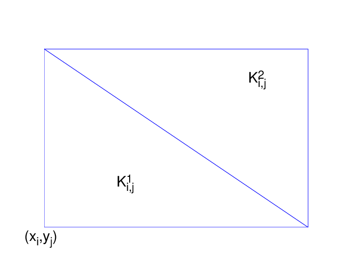
Figure 2: Ki,j1K^{1}_{i,j} and Ki,j2K^{2}_{i,j}

Next, we define the set of mesh points {(xi,yj)∈Ω:i,j=0,⋯,N}\left\{(x_{i},y_{j})\in\Omega:i,\,j=0,\,\cdots,\,N\right\}

xi=\displaystyle x_{i}= 2​i​(1−λx)/N\displaystyle 2i(1-\lambda_{x})/N for i=0,⋯,N/2i=0,\,\cdots,\,N/2,
xi=\displaystyle x_{i}= 1−2​(N−i)​λx/N\displaystyle 1-2(N-i)\lambda_{x}/N for i=N/2+1,⋯,Ni=N/2+1,\,\cdots,\,N

and

yj=\displaystyle y_{j}= 2​j​(1−λy)/N\displaystyle 2j(1-\lambda_{y})/N for j=0,⋯,N/2j=0,\,\cdots,\,N/2,
yj=\displaystyle y_{j}= 1−2​(N−j)​λy/N\displaystyle 1-2(N-j)\lambda_{y}/N for j=N/2+1,⋯,Nj=N/2+1,\,\cdots,\,N.

By drawing lines through these mesh points parallel to the xx-axis and yy-axis the domain Ω\Omega is partitioned into rectangles. Each rectangle is divided into two triangles by drawing the diagonal. This yields a triangulation of Ω\Omega denoted by 𝒯N\mathcal{T}_{N}(see Fig. 1). The mesh sizes hx,i:=xi+1−xih_{x,i}:=x_{i+1}-x_{i} and hy,j:=yj+1−yjh_{y,j}:=y_{j+1}-y_{j} satisfy

hx,i=\displaystyle h_{x,i}= Hx:=1−λxN/2\displaystyle H_{x}:=\frac{1-\lambda_{x}}{N/2} for i=0,⋯,N/2−1i=0,\,\cdots,\,N/2-1,
hx,i=\displaystyle h_{x,i}= hx:=λxN/2\displaystyle h_{x}:=\frac{\lambda_{x}}{N/2} for i=N/2,⋯,N−1i=N/2,\,\cdots,\,N-1

and

hy,j=\displaystyle h_{y,j}= Hy:=1−λyN/2\displaystyle H_{y}:=\frac{1-\lambda_{y}}{N/2} for j=0,⋯,N/2−1j=0,\,\cdots,\,N/2-1,
hy,j=\displaystyle h_{y,j}= hy:=λyN/2\displaystyle h_{y}:=\frac{\lambda_{y}}{N/2} for j=N/2,⋯,N−1j=N/2,\,\cdots,\,N-1.

The mesh sizes Hx,Hy,hxH_{x},H_{y},h_{x} and hyh_{y} satisfy

N−1≤Hx,Hy≤2N−1andC1εN−1lnN≤hx,hy≤C2εN−1lnN.N^{-1}\leq H_{x},H_{y}\leq 2N^{-1}\quad\mbox{and}\quad C_{1}\varepsilon N^{-1}\ln N\leq h_{x},h_{y}\leq C_{2}\varepsilon N^{-1}\ln N.

For convenience, we shall use the following notations: Ki,j1K^{1}_{i,j} for the mesh triangle with vertices (xi,yj)(x_{i},y_{j}), (xi+1,yj)(x_{i+1},y_{j}), and (xi,yj+1)(x_{i},y_{j+1}); Ki,j2K^{2}_{i,j} for the mesh triangle with vertices (xi,yj+1)(x_{i},y_{j+1}), (xi+1,yj)(x_{i+1},y_{j}), and (xi+1,yj+1)(x_{i+1},y_{j+1}) (see Fig. 2); KK for a generic mesh triangle.

On the above Shishkin meshes we define a C0C^{0} linear finite element space

VN:={vN∈C⁡(Ω¯):vN|∂Ω=0​ and vN|K∈P1​(K), ​∀K∈𝒯N}.V^{N}:=\{v^{N}\in C(\bar{\Omega}):v^{N}|_{\partial\Omega}=0\text{ and $v^{N}|_{K}\in P_{1}(K)$, }\forall K\in\mathcal{T}_{N}\}.

Now we are in a position to state the SDFEM. Let V:=H01​(Ω)V:=H^{1}_{0}(\Omega) and define the bilinear forms

aG​a​l​(v,w)\displaystyle a_{Gal}(v,w) =ε(∇v,∇w)+(𝒃⋅∇v,w)+(cv,w)v,w∈V;\displaystyle=\varepsilon(\nabla v,\nabla w)+(\boldsymbol{b}\cdot\nabla v,w)+(cv,w)\quad v,w\in V;
as​t​a​b​(v,w)\displaystyle a_{stab}(v,w) =∑K⊂Ω(−ε​Δ​v+𝒃⋅∇v+c​v,δK​𝒃⋅∇w)Kv∈V∩H2​(𝒯N),w∈V;\displaystyle=\sum_{K\subset\Omega}(-\varepsilon\Delta v+\boldsymbol{b}\cdot\nabla v+cv,\delta_{K}\boldsymbol{b}\cdot\nabla w)_{K}\quad v\in V\cap H^{2}(\mathcal{T}_{N}),\;w\in V;
aS​D​(v,w)\displaystyle a_{SD}(v,w) =aG​a​l​(v,w)+as​t​a​b​(v,w)v∈V∩H2​(𝒯N),w∈V,\displaystyle=a_{Gal}(v,w)+a_{stab}(v,w)\quad v\in V\cap H^{2}(\mathcal{T}_{N}),\;w\in V,

where H2(𝒯N)={v∈L2(Ω):∀K∈𝒯N,v|K∈H2(K)}H^{2}(\mathcal{T}_{N})=\{v\in L^{2}(\Omega):\forall K\in\mathcal{T}_{N},\;v|_{K}\in H^{2}(K)\}. The standard SDFEM reads:

{Find uN∈VN such that for all vN∈VN,aS​D​(uN,vN)=(f,vN)+∑K⊂Ω​(f,δK​𝒃⋅∇vN)K.\left\{\begin{array}[]{lr}\text{Find $u^{N}\in V^{N}$ such that for all $v^{N}\in V^{N}$},\\ a_{SD}(u^{N},v^{N})=(f,v^{N})+\underset{K\subset\Omega}{\sum}(f,\delta_{K}\boldsymbol{b}\cdot\nabla v^{N})_{K}.\end{array}\right. (2)

Note that Δ​uN=0\Delta u^{N}=0 in KK for uN|K∈P1​(K)u^{N}|_{K}\in P_{1}(K). Following usual practice [4], the parameter δK:=δ|K\delta_{K}:=\delta|_{K} is defined as follows:

δK={C∗​N−1if K⊂Ωs,0otherwise,\delta_{K}=\left\{\begin{array}[]{cc}C^{\ast}N^{-1}&\text{if $K\subset\Omega_{s}$},\\ 0&\text{otherwise},\end{array}\right. (3)

and C∗C^{\ast} is a properly defined positive constant such that the following coercivity holds (see [4, Lemma 3.25]):

aS​D(vN,vN)≥12⦀vN⦀2∀vN∈VN,a_{SD}(v^{N},v^{N})\geq\frac{1}{2}\vvvert v^{N}\vvvert^{2}\quad\forall v^{N}\in V^{N}, (4)

where

⦀vN⦀2:=ε|vN|21+∥vN∥2+∑K⊂ΩδK∥𝒃⋅∇vN∥2K.\vvvert v^{N}\vvvert^{2}:=\varepsilon|v^{N}|^{2}_{1}+\|v^{N}\|^{2}+\sum_{K\subset\Omega}\delta_{K}\|\boldsymbol{b}\cdot\nabla v^{N}\|^{2}_{K}. (5)

Coercivity (4) implies a unique solution of the discrete problem (2). Also the Galerkin orthogonality holds, i.e.,

aS​D​(u−uN,vN)=0∀vN∈VN.a_{SD}(u-u^{N},v^{N})=0\quad\forall v^{N}\in V^{N}. (6)

Set

b:=b12+b22,𝜷:=(b1b2)/b,𝜼:=(−b2b1)/b.b:=\sqrt{b^{2}_{1}+b^{2}_{2}},\quad\boldsymbol{\beta}:=\genfrac{(}{)}{0.0pt}{0}{b_{1}}{b_{2}}/b,\quad\boldsymbol{\eta}:=\genfrac{(}{)}{0.0pt}{0}{-b_{2}}{b_{1}}/b.

For our later analysis, we define a mesh subdomain of Ω\Omega for each mesh node 𝒙∗=(x∗,y∗)\boldsymbol{x}^{\ast}=(x^{*},y^{*}):

Ω0′:=Ω0′​(𝒙∗)={K∈𝒯N:meas​(Ω0∩K)≠0},\Omega^{\prime}_{0}:=\Omega^{\prime}_{0}(\boldsymbol{x}^{*})=\{K\in\mathcal{T}_{N}:\mbox{meas}(\Omega_{0}\cap K)\neq 0\}, (7)

where

Ω0:=Ω0(𝒙∗)={𝒙=(x,y)∈Ω:(𝒙−𝒙∗)⋅𝜷≤𝒦​σβ​ln⁡N​ and |(𝒙−𝒙∗)⋅𝜼|≤𝒦σηlnN}\begin{split}\Omega_{0}:=\Omega_{0}(\boldsymbol{x}^{*})=\big\{\boldsymbol{x}=(x,y)\in\Omega:&\;(\boldsymbol{x}-\boldsymbol{x}^{*})\cdot\boldsymbol{\beta}\leq\mathscr{K}\sigma_{\beta}\ln N\text{ and }\\ &|(\boldsymbol{x}-\boldsymbol{x}^{*})\cdot\boldsymbol{\eta}|\leq\mathscr{K}\sigma_{\eta}\ln N\big\}\end{split} (8)

(see Fig. 4 and Fig. 4) and

σβ=kN−1lnN,ση=kN−1/2.\sigma_{\beta}=kN^{-1}\ln N,\;\;\sigma_{\eta}=kN^{-1/2}. (9)

We shall choose k>0k>0 and 𝒦>0\mathscr{K}>0 later, which are independent of NN and ε\varepsilon. Note that

meas⁡(Ω0′)≤C​ση​ln⁡N.\mathrm{meas}(\Omega^{\prime}_{0})\leq C\sigma_{\eta}\ln N. (10)
Refer to caption
Figure 3: Subdomain Ω0=Ω0​(𝒙∗)\Omega_{0}=\Omega_{0}(\boldsymbol{x}^{*})
Refer to caption
Figure 4: Subdomain Ω0′=Ω0′​(𝒙∗)\Omega^{\prime}_{0}=\Omega^{\prime}_{0}(\boldsymbol{x}^{*})

2 The discrete Green’s function

In this section, we introduce the discrete Green’s function and cite some results from [2].

Let 𝒙∗=(x∗,y∗)\boldsymbol{x}^{\ast}=(x^{*},y^{*}) be a mesh node in Ω\Omega. The discrete Green’s function G∈VNG\in V^{N} associated with 𝒙∗\boldsymbol{x}^{\ast} is defined by

aS​D​(vN,G)=vN​(𝒙∗)∀vN∈VN.a_{SD}(v^{N},G)=v^{N}(\boldsymbol{x}^{\ast})\quad\forall v^{N}\in V^{N}. (11)

In the following analysis, we present the energy estimation of discrete Green’s functions. Our analysis is similar to that of [2], with some changes.

We define a weight function

ω⁡(𝒙):=g⁡((𝒙−𝒙∗)⋅𝜷σβ)​g​((𝒙−𝒙∗)⋅𝜼ση)​g​(−(𝒙−𝒙∗)⋅𝜼ση)\omega(\boldsymbol{x}):=g\left(\frac{(\boldsymbol{x}-\boldsymbol{x}^{\ast})\cdot\boldsymbol{\beta}}{\sigma_{\beta}}\right)g\left(\frac{(\boldsymbol{x}-\boldsymbol{x}^{\ast})\cdot\boldsymbol{\eta}}{\sigma_{\eta}}\right)g\left(-\frac{(\boldsymbol{x}-\boldsymbol{x}^{\ast})\cdot\boldsymbol{\eta}}{\sigma_{\eta}}\right)

with g⁡(r)=2/(1+er)g(r)=2/(1+e^{r}) for r∈(−∞,∞)r\in(-\infty,\infty). We shall choose k>0k>0 later. Note Lemma 4.1 in [2] holds if σβ≥k​N−1​ln⁡N\sigma_{\beta}\geq kN^{-1}\ln N and ση≥kN−1/2\sigma_{\eta}\geq kN^{-1/2}.

Now we define a weighted energy norm

⦀G⦀2ω:=ε∥ω−1/2Gβ∥2+ε∥ω−1/2Gη∥2+b2∥(ω−1)1/2βG∥2+c∥ω−1/2G∥2+∑Kb2δK∥ω−1/2Gβ∥2K.\begin{split}\vvvert G\vvvert^{2}_{\omega}:=&\varepsilon\|\omega^{-1/2}G_{\beta}\|^{2}+\varepsilon\|\omega^{-1/2}G_{\eta}\|^{2}+\frac{b}{2}\|(\omega^{-1})^{1/2}_{\beta}G\|^{2}\\ &+c\|\omega^{-1/2}G\|^{2}+\sum_{K}b^{2}\delta_{K}\|\omega^{-1/2}G_{\beta}\|^{2}_{K}.\end{split} (12)

Note that (ω−1)β>0(\omega^{-1})_{\beta}>0. For any subdomain DD of Ω\Omega, let ⦀G⦀ω,D\vvvert G\vvvert_{\omega,D} mean that the integrations in (12) are restricted to DD. From (2), (12) and integration by parts, we have

⦀G⦀2ω=aS​D​(ω−1​G,G)−ε⁡((ω−1)β​G,Gβ)−ε⁡((ω−1)η​G,Gη)−∑K(b(ω−1)βG+cω−1G,δKbGβ)K.\begin{split}\vvvert G\vvvert^{2}_{\omega}=&a_{SD}(\omega^{-1}G,G)-\varepsilon((\omega^{-1})_{\beta}G,G_{\beta})-\varepsilon((\omega^{-1})_{\eta}G,G_{\eta})\\ &-\sum_{K}(b(\omega^{-1})_{\beta}G+c\omega^{-1}G,\delta_{K}\;bG_{\beta})_{K}.\end{split}

Considering (11), we have

aS​D​(ω−1​G,G)=aS​D​(ω−1​G−(ω−1​G)I,G)+aS​D​((ω−1​G)I,G)=aS​D​(ω−1​G−(ω−1​G)I,G)+(ω−1​G)​(𝒙∗).\begin{split}a_{SD}(\omega^{-1}G,G)&=a_{SD}(\omega^{-1}G-(\omega^{-1}G)^{I},G)+a_{SD}((\omega^{-1}G)^{I},G)\\ &=a_{SD}(\omega^{-1}G-(\omega^{-1}G)^{I},G)+(\omega^{-1}G)(\boldsymbol{x}^{\ast}).\end{split}

By means of the above two equalities, the energy estimate of GG will be obtained from the next three Lemmas.

Lemma 1.

Assume σβ≥k​N−1\sigma_{\beta}\geq kN^{-1} and ση≥k​ε1/2\sigma_{\eta}\geq k\varepsilon^{1/2} in (8), then for k>1k>1 sufficiently large and independent of NN and ε\varepsilon, we have

aS​D(ω−1G,G)≥14⦀G⦀ω2.a_{SD}(\omega^{-1}G,G)\geq\frac{1}{4}\vvvert G\vvvert^{2}_{\omega}.
Proof.

See [2, Lemma 4.2]. ∎

Lemma 2.

If σβ≥k​N−1\sigma_{\beta}\geq kN^{-1} in (8), with k>0k>0 independent of NN and ε\varepsilon, then for each mesh point 𝐱∗∈Ω∖Ωx​y\boldsymbol{x}^{\ast}\in\Omega\setminus\Omega_{xy}, we have

|(ω−1G)(𝒙∗)|≤116⦀G⦀ω2+{C​N2​σβif 𝒙∗∈ΩsC​N​ln⁡Nif 𝒙∗∈Ωx∪Ωy.\left|(\omega^{-1}G)(\boldsymbol{x}^{\ast})\right|\leq\frac{1}{16}\vvvert G\vvvert^{2}_{\omega}+\left\{\begin{matrix}CN^{2}\sigma_{\beta}&\text{if $\boldsymbol{x}^{*}\in\Omega_{s}$}\\ CN\ln N&\text{if $\boldsymbol{x}^{*}\in\Omega_{x}\cup\Omega_{y}$}\end{matrix}\right..

where CC is independent of NN, ε\varepsilon and 𝐱∗\boldsymbol{x}^{\ast}.

Proof.

See [2, Lemma 4.3]. ∎

Lemma 3.

If σβ≥k​N−1​ln⁡N\sigma_{\beta}\geq kN^{-1}\ln N and ση≥kN−1/2\sigma_{\eta}\geq kN^{-1/2} in (8), where k>1k>1 is sufficiently large and independent of NN and ε\varepsilon, then

aS​D((ω−1G)I−ω−1G,G)≤116⦀G⦀ω2.a_{SD}((\omega^{-1}G)^{I}-\omega^{-1}G,G)\leq\frac{1}{16}\vvvert G\vvvert^{2}_{\omega}.
Proof.

For convenience we set E~​(𝒙):=((ω−1​G)I−ω−1​G)​(𝒙)\tilde{E}(\boldsymbol{x}):=((\omega^{-1}G)^{I}-\omega^{-1}G)(\boldsymbol{x}). Recall bb is constant and integration by parts yields (b​E~β,G)=−(b​E~,Gβ)(b\tilde{E}_{\beta},G)=-(b\tilde{E},G_{\beta}). Then we have

|aS​D​(E~,G)|≤C⁡(CLOSE‖(ε+b2​δ)1/2​ω1/2​E~β‖+ε1/2​‖ω1/2​E~η‖+∥(ε+b2δ)−1/2ω1/2E~∥)⦀G⦀ω.\begin{split}|a_{SD}(\tilde{E},G)|\leq C\big(&\|(\varepsilon+b^{2}\delta)^{1/2}\omega^{1/2}\tilde{E}_{\beta}\|+\varepsilon^{1/2}\|\omega^{1/2}\tilde{E}_{\eta}\|\\ &+\|(\varepsilon+b^{2}\delta)^{-1/2}\omega^{1/2}\tilde{E}\|\big)\vvvert G\vvvert_{\omega}.\end{split} (13)

To analyze different kinds of interpolation bounds, we first estimate the following terms. Note that Gβ​β=Gη​η=Gβ​η=0G_{\beta\beta}=G_{\eta\eta}=G_{\beta\eta}=0 on KK because GG belongs to VNV^{N}. For convenience, we set MK:=max𝐾ω−1/2M_{K}:=\underset{K}{\max}\,\omega^{-1/2}. Using (iii), (iv) and (v) in [2, Lemma 4.1], we obtain

‖(ω−1​G)β​β‖K≤‖(ω−1)β​β​G‖K+‖(ω−1)β​Gβ‖K≤CMK(σ−3/2β∥(ω−1)1/2βG∥K+σ−1β∥ω−1/2Gβ∥K)≤CMK(σ−3/2β+σ−1β(ε+b2δ)−1/2)⦀G⦀ω,K.\begin{split}&\|(\omega^{-1}G)_{\beta\beta}\|_{K}\leq\|(\omega^{-1})_{\beta\beta}G\|_{K}+\|(\omega^{-1})_{\beta}G_{\beta}\|_{K}\\ \leq&CM_{K}\left(\sigma^{-3/2}_{\beta}\|(\omega^{-1})^{1/2}_{\beta}G\|_{K}+\sigma^{-1}_{\beta}\|\omega^{-1/2}G_{\beta}\|_{K}\right)\\ \leq&CM_{K}\left(\sigma^{-3/2}_{\beta}+\sigma^{-1}_{\beta}(\varepsilon+b^{2}\delta)^{-1/2}\right)\vvvert G\vvvert_{\omega,K}.\end{split} (14)

Note ‖Gη‖K≤C​max⁡{hx,K−1,hy,K−1}​‖G‖K\|G_{\eta}\|_{K}\leq C\max\{h^{-1}_{x,K},h^{-1}_{y,K}\}\|G\|_{K} or ∥Gη∥K≤Cε−1/2⋅ε1/2∥Gη∥K\|G_{\eta}\|_{K}\leq C\varepsilon^{-1/2}\cdot\varepsilon^{1/2}\|G_{\eta}\|_{K}, then we have

∥Gη∥K≤Cmin{max{hx,K−1,hy,K−1},ε−1/2}⦀G⦀K,\|G_{\eta}\|_{K}\leq C\min\{\max\{h^{-1}_{x,K},h^{-1}_{y,K}\},\varepsilon^{-1/2}\}\vvvert G\vvvert_{K},

and

‖(ω−1)η​Gη‖K≤C​max𝐾​|(ω−1)η|​‖Gη‖K≤CMKσ−1ηmax𝐾ω−1/2⋅min{max{h−1x,K,h−1y,K},ε−1/2}⦀G⦀K≤CMKσ−1ηmin{max{h−1x,K,h−1y,K},ε−1/2}⦀G⦀ω,K.\begin{split}&\|(\omega^{-1})_{\eta}G_{\eta}\|_{K}\leq C\underset{K}{\max}|(\omega^{-1})_{\eta}|\;\|G_{\eta}\|_{K}\\ \leq&CM_{K}\sigma^{-1}_{\eta}\underset{K}{\max}\omega^{-1/2}\cdot\min\{\max\{h^{-1}_{x,K},h^{-1}_{y,K}\},\varepsilon^{-1/2}\}\vvvert G\vvvert_{K}\\ \leq&CM_{K}\sigma^{-1}_{\eta}\min\{\max\{h^{-1}_{x,K},h^{-1}_{y,K}\},\varepsilon^{-1/2}\}\vvvert G\vvvert_{\omega,K}.\end{split} (15)

Similarly, we have ∥(ω−1)η​ηG∥K≤CMKση−2∥ω−1/2G∥K\|(\omega^{-1})_{\eta\eta}G\|_{K}\leq CM_{K}\sigma^{-2}_{\eta}\|\omega^{-1/2}G\|_{K} and

‖(ω−1​G)η​η‖K≤‖(ω−1)η​η​G‖K+‖(ω−1)η​Gη‖K≤CMK(σ−2η+σ−1ηmin{max{h−1x,K,h−1y,K},ε−1/2})⦀G⦀ω,K.\begin{split}&\|(\omega^{-1}G)_{\eta\eta}\|_{K}\leq\|(\omega^{-1})_{\eta\eta}G\|_{K}+\|(\omega^{-1})_{\eta}G_{\eta}\|_{K}\\ \leq&CM_{K}\left(\sigma^{-2}_{\eta}+\sigma^{-1}_{\eta}\min\{\max\{h^{-1}_{x,K},h^{-1}_{y,K}\},\varepsilon^{-1/2}\}\right)\vvvert G\vvvert_{\omega,K}.\end{split} (16)

Recalling (v) in [2, Lemma 4.1] and inverse estimates, we have

‖(ω−1)β​Gη‖K≤C​max𝐾​(ω−1)β⋅‖Gη‖K≤C​max𝐾​(ω−1)β⋅max⁡{hx,K−1,hy,K−1}⋅‖G‖K≤C​max⁡{hx,K−1,hy,K−1}​(max𝐾​(ω−1)β)1/2​(min𝐾​(ω−1)β)1/2⋅‖G‖K≤CMK⋅max{h−1x,K,h−1y,K}σ−1/2β⋅∥(ω−1)1/2βG∥K.\begin{split}&\|(\omega^{-1})_{\beta}G_{\eta}\|_{K}\leq C\underset{K}{\max}(\omega^{-1})_{\beta}\cdot\|G_{\eta}\|_{K}\\ \leq&C\underset{K}{\max}(\omega^{-1})_{\beta}\cdot\max\{h^{-1}_{x,K},h^{-1}_{y,K}\}\cdot\|G\|_{K}\\ \leq&C\max\{h^{-1}_{x,K},h^{-1}_{y,K}\}\left(\underset{K}{\max}(\omega^{-1})_{\beta}\right)^{1/2}\left(\underset{K}{\min}(\omega^{-1})_{\beta}\right)^{1/2}\cdot\|G\|_{K}\\ \leq&CM_{K}\cdot\max\{h^{-1}_{x,K},h^{-1}_{y,K}\}\sigma^{-1/2}_{\beta}\cdot\|(\omega^{-1})^{1/2}_{\beta}G\|_{K}.\end{split} (17)

Also, we have

∥(ω−1)βGη∥K≤CMK⋅ε−1/2σβ−1⋅ε1/2∥ω−1/2Gη∥K.\|(\omega^{-1})_{\beta}G_{\eta}\|_{K}\leq CM_{K}\cdot\varepsilon^{-1/2}\sigma^{-1}_{\beta}\cdot\varepsilon^{1/2}\|\omega^{-1/2}G_{\eta}\|_{K}. (18)

Then from (17) and (18), we have

∥(ω−1)βGη∥K≤CMKmin{max{hx,K−1,hy,K−1}σβ−1/2,ε−1/2σβ−1}⦀G⦀ω,K,\|(\omega^{-1})_{\beta}G_{\eta}\|_{K}\leq CM_{K}\min\{\max\{h^{-1}_{x,K},h^{-1}_{y,K}\}\sigma^{-1/2}_{\beta},\varepsilon^{-1/2}\sigma^{-1}_{\beta}\}\vvvert G\vvvert_{\omega,K},

and then

‖(ω−1​G)β​η‖K≤‖(ω−1)β​η​G‖K+‖(ω−1)η​Gβ‖K+‖(ω−1)β​Gη‖K≤CMK(σ−1/2βσ−1η∥(ω−1)1/2βG∥K+σ−1η∥ω−1/2Gβ∥K)+∥(ω−1)βGη∥K≤CMK(σ−1/2βσ−1η+σ−1η(ε+b2δ)−1/2+min{max{h−1x,K,h−1y,K}σ−1/2β,ε−1/2σ−1β})⦀G⦀ω,K.\begin{split}&\|(\omega^{-1}G)_{\beta\eta}\|_{K}\leq\|(\omega^{-1})_{\beta\eta}G\|_{K}+\|(\omega^{-1})_{\eta}G_{\beta}\|_{K}+\|(\omega^{-1})_{\beta}G_{\eta}\|_{K}\\ \leq&CM_{K}\left(\sigma^{-1/2}_{\beta}\sigma^{-1}_{\eta}\|(\omega^{-1})^{1/2}_{\beta}G\|_{K}+\sigma^{-1}_{\eta}\|\omega^{-1/2}G_{\beta}\|_{K}\right)+\|(\omega^{-1})_{\beta}G_{\eta}\|_{K}\\ \leq&CM_{K}\big(\sigma^{-1/2}_{\beta}\sigma^{-1}_{\eta}+\sigma^{-1}_{\eta}(\varepsilon+b^{2}\delta)^{-1/2}\\ &+\min\{\max\{h^{-1}_{x,K},h^{-1}_{y,K}\}\sigma^{-1/2}_{\beta},\varepsilon^{-1/2}\sigma^{-1}_{\beta}\}\big)\vvvert G\vvvert_{\omega,K}.\end{split} (19)

Set hK=max⁡{hx,K,hy,K}h_{K}=\max\{h_{x,K},h_{y,K}\} and M~K:=(max𝐾​ω)1/2\tilde{M}_{K}:=(\underset{K}{\max}\omega)^{1/2}. From [2, Corollary 3.1], we have

‖ω1/2​E~‖K+hK​‖ω1/2​E~β‖K+hK​‖ω1/2​E~η‖K≤C​M~K​hK2​(‖(ω−1​G)β​β‖K+‖(ω−1​G)β​η‖K+‖(ω−1​G)η​η‖K).\begin{split}&\|\omega^{1/2}\tilde{E}\|_{K}+h_{K}\|\omega^{1/2}\tilde{E}_{\beta}\|_{K}+h_{K}\|\omega^{1/2}\tilde{E}_{\eta}\|_{K}\\ \leq&C\tilde{M}_{K}h^{2}_{K}\left(\|(\omega^{-1}G)_{\beta\beta}\|_{K}+\|(\omega^{-1}G)_{\beta\eta}\|_{K}+\|(\omega^{-1}G)_{\eta\eta}\|_{K}\right).\end{split} (20)

Substituting (14), (16) and (19) into (20), we have

(ε+b2​δ)​‖ω1/2​E~β‖2+ε​‖ω1/2​E~η‖2\displaystyle(\varepsilon+b^{2}\delta)\|\omega^{1/2}\tilde{E}_{\beta}\|^{2}+\varepsilon\|\omega^{1/2}\tilde{E}_{\eta}\|^{2} ≤Ck−2⦀G⦀2ω.\displaystyle\leq Ck^{-2}\vvvert G\vvvert^{2}_{\omega}. (21)

More precisely, we have

‖ω1/2​E~β‖Ωx≤Ck−1N−1(σ−1βε−1/2+σ−2η+σ−1ηε−1/2)⦀G⦀ω≤Ck−1ε−1/2ln−1N⦀G⦀ω.\begin{split}\|\omega^{1/2}\tilde{E}_{\beta}\|_{\Omega_{x}}\leq&Ck^{-1}N^{-1}(\sigma^{-1}_{\beta}\varepsilon^{-1/2}+\sigma^{-2}_{\eta}+\sigma^{-1}_{\eta}\varepsilon^{-1/2})\vvvert G\vvvert_{\omega}\\ \leq&Ck^{-1}\varepsilon^{-1/2}\ln^{-1}N\vvvert G\vvvert_{\omega}.\end{split} (22)

Substituting (14), (16) and (19) into (20) again, we have

‖ω1/2​E~‖K≤{Ck−1N−1/2⦀G⦀ω,Kif K⊂ΩsCk−1ε1/2⦀G⦀ω,Kif K⊂Ωx​y,\|\omega^{1/2}\tilde{E}\|_{K}\leq\left\{\begin{array}[]{ll}Ck^{-1}N^{-1/2}\vvvert G\vvvert_{\omega,K}&\text{if $K\subset\Omega_{s}$}\\ Ck^{-1}\varepsilon^{1/2}\vvvert G\vvvert_{\omega,K}&\text{if $K\subset\Omega_{xy}$}\end{array}\right., (23)

and

∥ω1/2E~∥K≤Ck−1ε−1/2N−1ln−1N⦀G⦀ω,Kif K⊂Ωx∪Ωy.\|\omega^{1/2}\tilde{E}\|_{K}\leq Ck^{-1}\varepsilon^{-1/2}N^{-1}\ln^{-1}N\vvvert G\vvvert_{\omega,K}\;\;\text{if $K\subset\Omega_{x}\cup\Omega_{y}$}. (24)

For what follows we need a sharper bound of ‖ω1/2​E~‖Ωx∪Ωy\|\omega^{1/2}\tilde{E}\|_{\Omega_{x}\cup\Omega_{y}}. Considering σβ≥k​N−1​ln⁡N\sigma_{\beta}\geq kN^{-1}\ln N, ση≥kN−1/2\sigma_{\eta}\geq kN^{-1/2}, (24) and (22), similar to [2, Lemma 4.4] we obtain

‖ω1/2​E~‖Ωx∪Ωy2≤C​λx2​{‖(ω1/2)β​E~‖Ωx∪Ωy2+‖ω1/2​E~β‖Ωx∪Ωy2}≤C​ε2​ln2​N⋅{σβ−2​‖ω1/2​E~‖Ωx∪Ωy2+‖ω1/2​E~β‖Ωx∪Ωy2}≤Ck−2ε2ln2N{σ−2βε−1N−2ln−2N+ε−1ln−2N}⦀G⦀2ω≤Ck−2ε⦀G⦀2ω.\begin{split}&\|\omega^{1/2}\tilde{E}\|^{2}_{\Omega_{x}\cup\Omega_{y}}\leq C\lambda^{2}_{x}\left\{\|(\omega^{1/2})_{\beta}\tilde{E}\|^{2}_{\Omega_{x}\cup\Omega_{y}}+\|\omega^{1/2}\tilde{E}_{\beta}\|^{2}_{\Omega_{x}\cup\Omega_{y}}\right\}\\ \leq&C\varepsilon^{2}\ln^{2}N\cdot\left\{\sigma^{-2}_{\beta}\|\omega^{1/2}\tilde{E}\|^{2}_{\Omega_{x}\cup\Omega_{y}}+\|\omega^{1/2}\tilde{E}_{\beta}\|^{2}_{\Omega_{x}\cup\Omega_{y}}\right\}\\ \leq&Ck^{-2}\varepsilon^{2}\ln^{2}N\{\sigma^{-2}_{\beta}\varepsilon^{-1}N^{-2}\ln^{-2}N+\varepsilon^{-1}\ln^{-2}N\}\vvvert G\vvvert^{2}_{\omega}\\ \leq&Ck^{-2}\varepsilon\vvvert G\vvvert^{2}_{\omega}.\end{split} (25)

Substituting (21), (23) and (25) into (13) and recalling the definition of δ\delta, we obtain

|aS​D(E~,G)|≤Ck−1⦀G⦀ω2.|a_{SD}(\tilde{E},G)|\leq Ck^{-1}\vvvert G\vvvert^{2}_{\omega}.

Choosing kk sufficiently large independently of ε\varepsilon and NN, we are done. ∎

Lemmas 1, 2 and 3 yield the following bound of the discrete Green function in the energy norm just as in [2, Theorem 4.1].

Theorem 1.

Assume that σβ=k​N−1​ln⁡N\sigma_{\beta}=kN^{-1}\ln N and ση=kN−1/2\sigma_{\eta}=kN^{-1/2} in (8), where kk is chosen so that Lemmas 1, 2 and 3 hold. Then for 𝐱∗∈Ω∖Ωx​y\boldsymbol{x}^{\ast}\in\Omega\setminus\Omega_{xy}, we have

⦀G⦀≤8⦀G⦀ω≤CN1/2ln1/2N.\vvvert G\vvvert\leq\sqrt{8}\vvvert G\vvvert_{\omega}\leq CN^{1/2}\ln^{1/2}N.
Remark 1.

For different crosswind diffusion coefficients, for example ε^\hat{\varepsilon} in [2] and ε\varepsilon in the present paper, we can choose σβ\sigma_{\beta} and ση\sigma_{\eta} large enough such that Lemmas 1–3 hold true. Thus with different assumptions on these parameters and different SDFEMs, we can obtain bounds similar to [2, Theorem 4.1], i.e., Theorem 1.

References

  • [1] T. Linß. Layer-adapted meshes for reaction-convection-diffusion problems, volume 1985 of Lecture Notes in Mathematics. Springer-Verlag, Berlin, 2010.
  • [2] T. Linß and M. Stynes. The SDFEM on Shishkin meshes for linear convection–diffusion problems. Numer. Math., 87(3):457–484, 2001.
  • [3] H.-G. Roos. Layer-adapted grids for singular perturbation problems. ZAMM Z. Angew. Math. Mech., 78(5):291–309, 1998.
  • [4] H.-G. Roos, M. Stynes, and L. Tobiska. Robust Numerical Methods for Singularly Perturbed Differential Equations, volume 24 of Springer Series in Computational Mathematics. Springer-Verlag, Berlin, second edition, 2008.
  • [5] M. Stynes and L. Tobiska. The SDFEM for a convection-diffusion problem with a boundary layer: optimal error analysis and enhancement of accuracy. SIAM J. Numer. Anal., 41(5):1620–1642, 2003.
  • [6] Z. Zhang. Finite element superconvergence on Shishkin mesh for 2-D convection-diffusion problems. Math. Comp., 72(243):1147–1177, 2003.