\setupctable

botcap,mincapwidth=doinside= ,footerwidth

The matter power spectrum in redshift space using effective field theory

Lucía Fonseca de la Bella¹, Donough Regan¹, David Seery¹ and Shaun Hotchkiss² Affiliation: ¹ Astronomy Centre, University of Sussex, Falmer, Brighton BN1 9QH, UK
² Department of Physics, The University of Auckland, Private Bag 92019, Auckland, New Zealand Email: L.Fonseca-De-La-Bella@sussex.ac.uk Email: D.Regan@sussex.ac.uk Email: D.Seery@sussex.ac.uk Email: s.hotchkiss@auckland.ac.nz

Abstract

The use of Eulerian ‘standard perturbation theory’ to describe mass assembly in the early universe has traditionally been limited to modes with $k\lesssim 0.1h/\text{Mpc}$ at $z=0$ . At larger $k$ the SPT power spectrum deviates from measurements made using $N$ -body simulations. Recently, there has been progress in extending the reach of perturbation theory to larger $k$ using ideas borrowed from effective field theory. We revisit the computation of the redshift-space matter power spectrum within this framework, including for the first time the full one-loop time dependence. We use a resummation scheme proposed by Vlah et al. to account for damping of baryonic acoustic oscillations due to large-scale random motions and show that this has a significant effect on the multipole power spectra. We renormalize by comparison to a suite of custom $N$ -body simulations matching the MultiDark MDR1 cosmology. At $z=0$ and for scales $k\lesssim 0.4h/\text{Mpc}$ we find that the EFT furnishes a description of the real-space power spectrum up to $\sim 2\%$ , for the $\ell=0$ mode up to $\sim 5\%$ , and for the $\ell=2,4$ modes up to $\sim 25\%$ . We argue that, in the MDR1 cosmology, positivity of the $\ell=0$ mode gives a firm upper limit of $k\approx 0.74h/\text{Mpc}$ for the validity of the one-loop EFT prediction in redshift space using only the lowest-order counterterm. We show that replacing the one-loop growth factors by their Einstein-de Sitter counterparts is a good approximation for the $\ell=0$ mode, but can induce deviations as large as $2\%$ for the $\ell=2,4$ modes. An accompanying software bundle, distributed under open source licenses, includes Mathematica notebooks describing the calculation, together with parallel pipelines capable of computing both the necessary one-loop SPT integrals and the effective field theory counterterms.

1 Introduction

The long dominance of the cosmic microwave background (CMB) as our principal source of information regarding the early universe will soon come to an end, displaced by new datasets from large galaxy redshift surveys. In addition to present-day surveys such as the Dark Energy Survey, the list will expand over the next decade to include at least Euclid, the Dark Energy Spectroscopic Instrument, the Large Synoptic Survey Telescope, the Square Kilometer Array, and the 4-metre Multi Object Spectroscopic Telescope. The ensemble of Fourier modes visible to each of these instruments carries information about both (i) the gravitational potentials—presumably generated by inflation—that seeded structure formation, and (ii) the effective force laws that operated while matter was drawn into these potential wells and condensed into halos. This sensitivity to a rich range of physical processes means that the imminent era of large galaxy surveys should drive a step change in our understanding of the standard cosmological model—and especially its poorly-understood early- and late-time accelerating phases.

The price to be paid for access to this information is an obligation to connect our theoretical description with observation by carrying out sophisticated modelling of both gravitational potentials and force laws. Analytic control has traditionally come from the use of perturbation theory [1, 2, 3, 4, 5, 6, 7, 8], but its reach is limited in scale to $k\lesssim 0.1h/\text{Mpc}$ at $z=0$ and therefore excludes a significant fraction of the modes visible to the surveys listed above. Large $N$ -body simulations provide an alternative, but although Moore’s Law has significantly reduced their time cost they are still expensive—certainly too expensive to be considered routine for extensions of the standard cosmological model that entail a significant increase in the parameter space. These pressures have produced a large literature based on enhancements of standard perturbation theory (‘SPT’) that extend its reach to moderate $k$ in the approximate range $0.1h/\text{Mpc}$ to $0.5h/\text{Mpc}$ . One such approach is based on modern ideas from effective field theory [9, 10, 11, 12, 13, 14, 15, 16], leading to the so-called ‘effective field theory of large-scale structure’. This has yielded encouraging results for the matter power spectrum and bispectrum, at the cost of adjustable counterterms that must be estimated from observation or from $N$ -body simulations.

Redshift space effects.—In this paper we revisit the application of these ideas to the redshift-space power spectrum. Real surveys must estimate the radial distance to a source from its redshift, and therefore do not measure the galaxies’ true spatial configuration. Unknown peculiar velocities associated with each source bias our distance estimate, introducing a systematic ‘redshift space distortion’ that must be modelled appropriately if we are to extract reliable results [17]. This is both a challenge and an opportunity. While redshift-space effects complicate the analysis, they enable us to measure correlations between densities and velocities that carry information about the effective gravitational force law on cosmological scales. In Einstein gravity, for the non-relativistic regime applicable to large-scale structure, this effective force is composed of an attractive $1/r^{2}$ component that is offset by a repulsive contribution from the cosmological expansion. In non-Einstein gravities the competition between these effects may be altered, or the scale-dependence of the force law may itself be modified due to processes involving exchange of new force-carrying particles.

These non-Einstein gravities could be constrained by precise measurements of the effective force law on cosmological scales, but only if its scale-dependence can be separated from uncertainties in our computation of its behaviour in the standard cosmological model. For this purpose effective field theory should be a helpful tool, enabling us to extend the range of wavenumbers that can be reached analytically and used for comparison. Senatore & Zaldarriaga [14] and later Lewandowski et al. [18] provided an analysis of the redshift-space matter power spectrum within such an effective description. More recently, Perko et al. extended this analysis to include biased tracers of the dark matter distribution [19] (see also Refs. [20, 21]). By itself, the dark matter can be measured only through its impact on cosmological weak lensing.

In this paper we revisit the redshift-space analysis for the pure matter power spectrum. Our computation is similar to that of Lewandowski et al., with which it shares a common language and point of departure. However, it differs in certain technical details such as construction of the counterterms, our procedure for estimating their numerical values, and our procedure to resum large loop-level terms involving integrals over the infrared part of the power spectrum. Moreover, we compute all time dependent terms exactly. Because these time dependences are known to be relatively insensitive to cosmology they are often approximated as powers of the Einstein–de Sitter growth function $D(z)$ . Since we retain the full time dependence we are able to assess the accuracy of the Einstein--de Sitter approximation.¹¹ 1 Bose & Koyama introduced a software tool that can numerically integrate the one-loop power spectrum in redshift space for a variety of models [22, 23]. Exact time dependence is sometimes considered in analytic calculations; eg., for recent examples, see Refs. [24, 25]. Fasiello & Vlah quoted exact results for cosmologies more general than $\Lambda$ CDM, but because they did not commit to a specific scenario their results were expressed as quadratures [24]. Closed-form analytic expressions for the one-loop $\Lambda$ CDM power spectrum in redshift space have not previously been given.

This enables us to assess the accuracy of the Einstein–de Sitter approximation. We renormalize to a suite of custom $N$ -body simulations performed using the gevolution numerical relativity code.

As part of our analysis we describe some computational innovations that we believe to be improvements over the traditional methods used by Matsubara to compute the redshift-space power spectrum in standard perturbation theory [26]. One such innovation is an algorithm to extract the explicit $\mu$ -dependence²² 2 Here, $\mu=\hat{\bm{\mathrm{{k}}}}\cdot\hat{\bm{\mathrm{{n}}}}$ is the orientation of a $\bm{\mathrm{{k}}}$ mode contributing to the matter density field relative to the line of sight $\hat{\bm{\mathrm{{n}}}}$ from Earth. of the redshift-space power spectrum using the Rayleigh plane-wave expansion and analytic formulae for weighted integrals over products of two or three spherical Bessel functions. A procedure to compute these three-Bessel integrals was described by Gervois & Navelet [27], and more recently by Fabrikant [28]. However, their results do not yet seem to have entered the cosmological literature.³³ 3 Certain three-Bessel integrals were computed as long ago as 1936 by Bailey [29]. However, Bailey’s method (and its descendents) required a triangle inequality to be satisfied by the arguments of the Bessel functions. To be effective our algorithm requires knowledge of the integral for any values of the arguments and not just those that satisfy the triangle inequality. It is for this extension that we require the more advanced methods of Refs. [27, 28].

Code availability.—To assist those who wish to replicate or extend our analysis, we have made our computer codes and supporting datasets available as part of a software bundle accompanying this paper. These include the parameter files needed to reconstruct our initial linear power spectra, the settings files required to reproduce our gevolution simulations, and databases containing the loop integrals and one-loop power spectra evaluated using the EFT. Each of these products can be downloaded by following the links given in Appendix C.

Summary.—Our presentation is organized as follows. In §2 we fix notation by summarizing the construction of the renormalized real-space matter power spectrum, originally described by Carrasco et al. [10, 11]. In §2.1 we collect the equations of structure formation during the matter era and describe their non-relativistic limit. In §2.2 we construct Eulerian perturbation theory based on these equations and compute the one-loop correction to the power spectrum of the density contrast $\delta=\delta\rho/\rho$ . The time-dependent factors $D_{A},\ldots,D_{J}$ and the loop integrals $P_{AA},\ldots,P_{BB},P_{D},\ldots,P_{J_{1}},P_{J_{2}}$ are the key results from this section. They are re-used extensively in §3.

In §2.3 we briefly summarize the use of effective field-theory methods to parametrize the unknown ultraviolet parts of these loop integrals. In §2.4 we describe renormalization of the velocity field, and explain how to relate the perspective used in this paper to the ‘smoothing’ prescription for renormalized operators used in Refs. [9, 10, 11, 30] and elsewhere. In §2.5 we introduce a scheme proposed by Vlah, Seljak, Chu & Feng to resum the damping effect of displacements on large scales and assess its impact on the real-space power spectrum. We conclude this section by describing the renormalization of the power spectrum at redshift $z=0$ (§2.6), and compare our results with those already reported in the literature.

This section can be read as a mini-primer on the use of effective field-theory methods. Readers already familiar with their application to large-scale structure may wish to focus on §2.2—which introduces our notation for time-dependent factors, the SPT kernels, and loop integrals—and §2.5, which describes our resummation prescription. These summarize the principal technical differences between our formalism and the existing literature.

In §3 we describe the renormalization of the redshift-space power spectrum. In §3.1 we write down an expression suitable for computing the redshift-space density contrast $\delta_{s}$ up to one-loop and discuss the counterterms needed to renormalize it. In §3.2 we describe the calculation of the $\delta_{s}$ power spectrum up to one-loop, introducing a new method to simplify evaluation of the tensor integrals that appear at this order. We extend the Vlah et al. resummation scheme to redshift space in §3.3 and comment on its relation to empirical schemes for capturing the suppression of power on small scales due to randomized virial motions within halos. In §3.4 we describe the construction of the Legendre multipoles. A significant advantage of the Vlah et al. resummation scheme is that this can be done analytically, reducing the requirement for expensive numerical computation. The $N$ -body simulations needed to obtain non-linear measurements of these multipoles are described in §3.5. We comment on a number of difficulties encountered when extracting reliable estimates of the redshift-space multipoles. Finally, in §3.6 we fit for the counterterms of the effective description and discuss the resulting power spectra. We assess the accuracy of the Einstein–de Sitter approximation and comment on the time-dependence of the EFT counterterms. We conclude in §4. A number of Appendices extend the discussion presented in the main text.

Notation.—We use units in which $c=\hbar=1$ and define the reduced Planck mass to be $M_{\mathrm{P}}=(8\pi G)^{-1/2}$ . Our Fourier convention is $f(\bm{\mathrm{{x}}})=\int\mathrm{d}^{3}k\,(2\pi)^{-3}\,f(\bm{\mathrm{{k}}})\mathrm{e}^{{\mathrm{i}\bm{\mathrm{{k}}}\cdot\bm{\mathrm{{x}}}}}$ .

Latin indices $a$ , $b$ , …, from the beginning of the alphabet range over spacetime coordinates $(t,x,y,z)$ or $(0,1,2,3)$ . Latin indices $i$ , $j$ , …, from the middle of the alphabet range over spatial indices only. Repeated spacetime indices are taken to be contracted with the metric $g_{ab}$ . Repeated spatial indices all in the ‘up’ or ‘down’ position are contracted with the three-dimensional Euclidean metric $\delta_{ij}$ , so that (for example) $v^{2}=v^{i}v^{i}=\delta_{ij}v^{i}v^{j}=\sum_{i}(v^{i})^{2}$ , and likewise for $v_{i}v_{i}=\delta^{ij}v_{i}v_{j}$ .

2 One-loop renormalization of the matter power spectrum in real space

In this section we briefly recapitulate the construction of the one-loop matter power spectrum, neglecting the complexities of redshift-space distortions. The material presented here is a review of the theory developed by Baumann et al. [9], Carrasco et al. [10, 11] and Mercolli & Pajer [30], although some results are new (including renormalization of the velocity accounting for its full time dependence), and parts of our presentation are different to discussions that have already appeared in the literature. We develop the formalism in detail because we will rely on the notation and methodology developed here when we study the power spectrum in redshift space.

2.1 Matter equations of motion

Initially we work in a non-linear Newtonian gauge for which the metric can be written

\mathrm{d}s^{2}=-\mathrm{e}^{{2\Psi}}\,\mathrm{d}t^{2}+a^{2}\,\mathrm{e}^{{2\Phi}}\,\mathrm{d}\bm{\mathrm{{x}}}^{2}.

(1)

The comoving dark matter velocity satisfies $u^{a}=\mathrm{e}^{{-\Psi}}\gamma(1,\bm{\mathrm{{v}}})$ , where $\gamma=(1-v_{\text{phys}}^{2})^{-1/2}$ is the special-relativistic Lorentz factor and $v_{\text{phys}}=a\mathrm{e}^{{\Phi-\Psi}}v$ is the physical peculiar 3-velocity. To obtain the true physical velocity for a source at distance $d$ we should add $v_{\text{phys}}$ to the Hubble flow $v_{\text{H}}=Hd$ . In this metric, the continuity equation for a perfect fluid with pressure $p$ and density $\rho$ can be written

\partial_{t}\Big(\gamma^{2}(p+\rho)-p\Big)+\nabla\cdot\Big(\gamma^{2}(p+\rho)\bm{\mathrm{{v}}}\Big)+\gamma^{2}(p+\rho)\Big(\bm{\mathrm{{v}}}\cdot\nabla(\Psi+3\Phi)+(H+\dot{\Phi})(4-\gamma^{-2})\Big)=0,

(2)

and the Euler equation is

\begin{split}\partial_{t}\Big(\gamma^{2}\bm{\mathrm{{v}}}(p+\rho)\Big)&+(\bm{\mathrm{{v}}}\cdot\nabla)\Big(\gamma^{2}\bm{\mathrm{{v}}}(p+\rho)\Big)+\frac{1}{a^{2}}\mathrm{e}^{{2\Psi-2\Phi}}\nabla p\\ &\mbox{}+\gamma^{2}\bm{\mathrm{{v}}}(p+\rho)\Big(\nabla\cdot\bm{\mathrm{{v}}}+5(H+\dot{\Phi})+5\bm{\mathrm{{v}}}\cdot\nabla\Phi-\bm{\mathrm{{v}}}\cdot\nabla\Psi-\dot{\Psi}\Big)\\ &\mbox{}+\frac{1}{a^{2}}\mathrm{e}^{{2\Psi-2\Phi}}(p+\rho)\Big(\gamma^{2}\nabla\Psi-(\gamma^{2}-1)\nabla\Phi\Big)=0.\end{split}

(3)

An overdot denotes a derivative with respect to time $t$ . The gravitational potentials satisfy the Poisson constraint,

\begin{split}\frac{1}{a^{2}}\nabla^{2}\Phi+\frac{1}{2a^{2}}\nabla\Phi\cdot\nabla\Phi=&\mbox{}-\frac{\mathrm{e}^{{2\Phi}}}{2M_{\mathrm{P}}^{2}}\Big(\gamma^{2}(p+\rho)-p-3Ha^{2}\mathrm{e}^{{-2\Psi}}\nabla^{-2}\nabla\cdot[\gamma^{2}\mathrm{e}^{{2\Phi}}(p+\rho)\bm{\mathrm{{v}}}]\Big)\\ &\mbox{}+\mathrm{e}^{{2\Phi-2\Psi}}\Big(\frac{3}{2}H^{2}+3H\nabla^{-2}[(H+\dot{\Phi})\nabla^{2}\Psi+\nabla\dot{\Phi}\cdot\nabla\Psi]+\frac{3}{2}\dot{\Phi}^{2}\Big).\end{split}

(4)

Finally, for Einstein gravity coupled to a perfect fluid, the gravitational potentials will be related by the no-slip condition $\Psi=-\Phi$ . All these equations are exact. In particular, they do not assume that the density and pressure are perturbatively small or that velocities are non-relativistic.

Non-relativistic limit.—Up to this point we have retained all terms in order to make clear what is entailed by our approximations. We wish to use these equations to describe deposition of matter by a gravitationally-driven flow within the potential wells associated with $\Phi$ and $\Psi$ . Assume that the flow carries density $\rho_{\text{f}}$ which is deposited onto a condensation of density $\rho_{\text{c}}$ . Therefore the density contrast $\delta$ is approximately $\rho_{\text{c}}/\rho_{\text{f}}$ . In a static Newtonian universe the flow velocity at distance $R$ from the condensation is roughly

v\sim\frac{R}{t_{\text{ff}}}\frac{\rho_{\text{c}}}{\rho_{\text{f}}}\sim\frac{R}{t_{\text{ff}}}\delta,

(5)

where $t_{\text{ff}}\approx(G\rho_{\text{f}})^{-1/2}$ is the free-fall time associated with the flow. This correlation between $v$ and $\delta$ is characteristic of an inverse-square-law force. It continues to apply in an expanding universe described by Einstein gravity, adjusted by a scale-independent constant of order unity that accounts for competition between Newtonian attraction and cosmological repulsion. In a non-Einstein gravity we should expect its $R$ dependence or the overall constant of proportionality to receive corrections. Ultimately, it is these corrections that we wish to explore using redshift-space distortions.

Returning to Einstein gravity and temporarily restoring factors of $c$ we conclude that $v/c$ scales like $t_{R}/t_{\text{ff}}$ , where $t_{R}=R/c$ is the light-crossing time at distance $R$ . In the case of cosmological structure formation the flow density $\rho_{\text{f}}$ is the background matter density and $t_{\text{ff}}$ is of order a Hubble time. Therefore $t_{R}/t_{\text{ff}}\ll 1$ on any scale well inside the Hubble radius, making $v/c\ll 1$ . On these scales it follows that relativistic corrections $\sim\BigO(\gamma)$ will be negligible. A similar discussion was given by Fry [3].

On the other hand, terms of order $\nabla\bm{\mathrm{{v}}}\sim t_{\text{ff}}^{-1}\rho_{\text{c}}/\rho_{\text{f}}$ need not be suppressed. In combination with a time derivative such as $\dot{\rho}$ or $\dot{\bm{\mathrm{{v}}}}$ the relative importance of such terms will be of order $t_{\text{ff}}\nabla\bm{\mathrm{{v}}}\sim\rho_{\text{c}}/\rho_{\text{f}}$ , which need not be especially small. Therefore it is meaningful to develop a series expansion in $\nabla\bm{\mathrm{{v}}}$ while neglecting relativistic corrections from terms of order $v^{2}$ and higher. This is standard perturbation theory or ‘SPT’. Specializing to matter domination, in which the gravitational potentials are determined by the matter density fluctuation, and keeping only terms linear in $\Phi=-\Psi$ , Eqs. (2)–(4) for pressureless cold dark matter reduce to


$\displaystyle\dot{\delta}+\nabla\cdot\Big((1+\delta)\bm{\mathrm{{v}}}\Big)$	$\displaystyle=0$	(6a)
$\displaystyle\dot{\bm{\mathrm{{v}}}}+(\bm{\mathrm{{v}}}\cdot\nabla)\bm{\mathrm{{v}}}+2H\bm{\mathrm{{v}}}-\frac{1}{a^{2}}\nabla\Phi$	$\displaystyle=0$	(6b)
$\displaystyle\frac{1}{a^{2}}\nabla^{2}\Phi$	$\displaystyle=-\frac{3H^{2}}{2}\Omega_{m}\delta,$	(6c)

where we have decomposed the density as $\rho=\rho_{0}+\delta\rho$ , with $\rho_{0}$ the homogeneous background, and $\delta=\delta\rho/\rho$ is the density contrast. The quantity $\Omega_{m}=\rho_{m}/(3H^{2}M_{\mathrm{P}}^{2})$ is the redshift-dependent matter density parameter.

Radial inflow approximation.—On large scales the flow $\bm{\mathrm{{v}}}$ will be oriented nearly radially into a nearby potential well and the vorticity $\bm{\mathrm{{\omega}}}=\nabla\times\bm{\mathrm{{v}}}$ will be very small. In this ‘potential flow’ region the velocity can be written as a gradient $\bm{\mathrm{{v}}}=\nabla\nabla^{-2}\theta$ , where $\theta=\nabla\cdot\bm{\mathrm{{v}}}$ is the velocity divergence. In this approximation, after translation to Fourier space, Eqs. (6a)–(6c) become


$\displaystyle\dot{\delta}_{\bm{\mathrm{{k}}}}+\theta_{\bm{\mathrm{{k}}}}$	$\displaystyle=-\int\frac{\mathrm{d}^{3}q\,\mathrm{d}^{3}s}{(2\pi)^{6}}\,(2\pi)^{3}\delta(\bm{\mathrm{{k}}}-\bm{\mathrm{{q}}}-\bm{\mathrm{{s}}})\alpha(\bm{\mathrm{{q}}},\bm{\mathrm{{s}}})\theta_{\bm{\mathrm{{q}}}}\delta_{\bm{\mathrm{{s}}}},$	(7a)
$\displaystyle\dot{\theta}_{\bm{\mathrm{{k}}}}-2H\dot{\theta}_{\bm{\mathrm{{k}}}}+\frac{3H^{2}}{2}\Omega_{m}\delta_{\bm{\mathrm{{k}}}}$	$\displaystyle=-\int\frac{\mathrm{d}^{3}q\,\mathrm{d}^{3}s}{(2\pi)^{6}}\,(2\pi)^{3}\delta(\bm{\mathrm{{k}}}-\bm{\mathrm{{q}}}-\bm{\mathrm{{s}}})\beta(\bm{\mathrm{{q}}},\bm{\mathrm{{s}}})\theta_{\bm{\mathrm{{q}}}}\theta_{\bm{\mathrm{{s}}}},$	(7b)

where the dimensionless kernels $\alpha(\bm{\mathrm{{q}}},\bm{\mathrm{{s}}})$ and $\beta(\bm{\mathrm{{q}}},\bm{\mathrm{{s}}})$ satisfy


$\displaystyle\alpha(\bm{\mathrm{{q}}},\bm{\mathrm{{s}}})$	$\displaystyle=\frac{\bm{\mathrm{{q}}}\cdot(\bm{\mathrm{{q}}}+\bm{\mathrm{{s}}})}{q^{2}},$	(8a)
$\displaystyle\beta(\bm{\mathrm{{q}}},\bm{\mathrm{{s}}})$	$\displaystyle=\frac{\bm{\mathrm{{q}}}\cdot\bm{\mathrm{{s}}}}{2q^{2}s^{2}}(\bm{\mathrm{{q}}}+\bm{\mathrm{{s}}})^{2}.$	(8b)

Notice that $\beta$ is symmetric but $\alpha$ is not. For future use it is helpful to define a symmetrized version of weight unity,

\bar{\alpha}(\bm{\mathrm{{q}}},\bm{\mathrm{{s}}})=\frac{1}{2}\alpha(\bm{\mathrm{{q}}},\bm{\mathrm{{s}}})+\frac{1}{2}\alpha(\bm{\mathrm{{s}}},\bm{\mathrm{{q}}}).

(9)

We also define a third kernel $\gamma(\bm{\mathrm{{q}}},\bm{\mathrm{{s}}})$ to be a sum of the $\alpha$ and $\beta$ kernels,

\gamma(\bm{\mathrm{{q}}},\bm{\mathrm{{s}}})=\alpha(\bm{\mathrm{{q}}},\bm{\mathrm{{s}}})+\beta(\bm{\mathrm{{q}}},\bm{\mathrm{{s}}}).

(10)

Like $\alpha$ , it can be symmetrized to give $\bar{\gamma}(\bm{\mathrm{{q}}},\bm{\mathrm{{s}}})$ . Observe that the linear part of Eq. (7a) reads $\theta_{\bm{\mathrm{{k}}}}=-\dot{\delta}_{\bm{\mathrm{{k}}}}$ , which replicates our conclusion above that $\nabla\bm{\mathrm{{v}}}\sim t_{\text{ff}}^{-1}\rho_{\text{c}}/\rho_{\text{f}}\sim H\delta$ .

Combining Eqs. (7a)–(7b) to eliminate $\theta_{\bm{\mathrm{{k}}}}$ and obtain a single second-order equation for $\delta_{\bm{\mathrm{{k}}}}$ , and exchanging cosmic time $t$ for redshift $z$ , defined by

1+z=\frac{a_{0}}{a},

(11)

where $a_{0}=a(t_{0})$ is the present-day value of the scale factor, we find

\begin{split}\delta_{\bm{\mathrm{{k}}}}^{\prime\prime}-\frac{1-\epsilon}{1+z}\delta_{\bm{\mathrm{{k}}}}^{\prime}&\mbox{}-\frac{3}{2}\frac{\Omega_{m}}{(1+z)^{2}}\delta_{\bm{\mathrm{{k}}}}\\ &=-\int\frac{\mathrm{d}^{3}q\,\mathrm{d}^{3}s}{(2\pi)^{6}}(2\pi)^{3}\delta(\bm{\mathrm{{k}}}-\bm{\mathrm{{q}}}-\bm{\mathrm{{s}}})S_{2}(\bm{\mathrm{{q}}},\bm{\mathrm{{s}}})\\ &\quad-\int\frac{\mathrm{d}^{3}q\,\mathrm{d}^{3}s}{(2\pi)^{6}}(2\pi)^{3}\delta(\bm{\mathrm{{k}}}-\bm{\mathrm{{q}}}-\bm{\mathrm{{s}}})\int\frac{\mathrm{d}^{3}t\,\mathrm{d}^{3}u}{(2\pi)^{6}}(2\pi)^{3}\delta(\bm{\mathrm{{s}}}-\bm{\mathrm{{t}}}-\bm{\mathrm{{u}}})S_{3}(\bm{\mathrm{{q}}},\bm{\mathrm{{s}}},\bm{\mathrm{{t}}},\bm{\mathrm{{u}}})\\ &\quad+\BigO(\delta^{4}).\end{split}

(12)

We have retained terms only up to $\BigO(\delta^{3})$ ; those of higher order do not contribute to the one-loop power spectrum. A prime ^′ denotes a derivative with respect to $z$ . The quantity $\epsilon$ is defined by $\epsilon=-\dot{H}/H^{2}$ and can be related to the deceleration parameter. The source terms $S_{2}$ and $S_{3}$ satisfy

S_{2}(\bm{\mathrm{{q}}},\bm{\mathrm{{s}}})=\bar{\gamma}(\bm{\mathrm{{q}}},\bm{\mathrm{{s}}})\delta^{\prime}_{\bm{\mathrm{{q}}}}\delta^{\prime}_{\bm{\mathrm{{s}}}}+\frac{3}{2}\frac{\Omega_{m}}{(1+z)^{2}}\bar{\alpha}(\bm{\mathrm{{q}}},\bm{\mathrm{{s}}})\delta_{\bm{\mathrm{{q}}}}\delta_{\bm{\mathrm{{s}}}},

(13)

and

S_{3}(\bm{\mathrm{{q}}},\bm{\mathrm{{s}}},\bm{\mathrm{{t}}},\bm{\mathrm{{u}}})=\alpha(\bm{\mathrm{{s}}},\bm{\mathrm{{q}}})\beta(\bm{\mathrm{{t}}},\bm{\mathrm{{u}}})\delta_{\bm{\mathrm{{q}}}}\delta^{\prime}_{\bm{\mathrm{{t}}}}\delta^{\prime}_{\bm{\mathrm{{u}}}}+2\beta(\bm{\mathrm{{q}}},\bm{\mathrm{{s}}})\alpha(\bm{\mathrm{{t}}},\bm{\mathrm{{u}}})\delta^{\prime}_{\bm{\mathrm{{q}}}}\delta^{\prime}_{\bm{\mathrm{{t}}}}\delta_{\bm{\mathrm{{u}}}}+\alpha(\bm{\mathrm{{s}}},\bm{\mathrm{{q}}})\alpha(\bm{\mathrm{{t}}},\bm{\mathrm{{u}}})\delta^{\prime}_{\bm{\mathrm{{q}}}}\delta^{\prime}_{\bm{\mathrm{{t}}}}\delta_{\bm{\mathrm{{u}}}}.

(14)

2.2 Eulerian perturbation theory

The most straightforward approach to solution of Eq. (12) is via an expansion in powers of $\delta$ . The outcome of this procedure is described as Eulerian perturbation theory.

Linear solution.—First consider the linear term, which does not require the sources $S_{2}$ and $S_{3}$ . Because Eq. (12) applies only during matter domination we should suppose the initial condition $\delta_{\bm{\mathrm{{k}}}}=\delta_{\bm{\mathrm{{k}}}}^{\ast}$ to be set at some redshift $z=z^{\ast}$ that is well within the matter era, but still early enough that terms of order $(\delta_{\bm{\mathrm{{k}}}}^{\ast})^{2}$ or higher can be neglected. For practical calculations we normally set $z^{\ast}\approx 50$ .

The linear solution is $\delta_{\bm{\mathrm{{k}}}}(z)=D(z)\delta_{\bm{\mathrm{{k}}}}^{\ast}$ , where the growth function $D(z)$ satisfies

D^{\prime\prime}-\frac{1-\epsilon}{1+z}D^{\prime}-\frac{3}{2}\frac{\Omega_{m}}{(1+z)^{2}}D=0.

(15)

If the initial time $z^{\ast}$ is chosen sufficiently early then the initial condition requires that $D(z)$ is approximately given by the matter-dominated solution $D(z)\approx a(z)/a(z^{\ast})$ . Notice that $D^{\ast}=D(z^{\ast})=1$ . Solutions to this equation were studied by Mészáros [31] and Groth & Peebles [32]. The velocity can be determined from the linear part of Eq. (7a), yielding

\theta_{\bm{\mathrm{{k}}}}=-fH\delta_{\bm{\mathrm{{k}}}}

(16)

where the growth factor $f(z)$ is defined to be

f\equiv-(1+z)\frac{D^{\prime}}{D}=\frac{\mathrm{d}\ln D}{\mathrm{d}\ln a}.

(17)

Eqs. (16)–(17) are nothing more than the estimate (5) in this model, with $t_{\text{ff}}=1/H$ and $R\sim 1/k$ , and $f$ representing a scale-independent damping of the gravitational force due to cosmological expansion. In the matter-only Einstein–de Sitter model we have $f=1$ and there is no damping of the correlation between $\bm{\mathrm{{v}}}$ and $\delta$ ; the effect of the expansion is only to soften exponential growth of $\delta$ into a power-law. For $\Omega_{m}<1$ there is extra suppression which can be estimated in Einstein gravity by $f\approx\Omega_{m}^{5/9}$ [33].

Second-order solution.—To distinguish the different contributions to $\delta_{\bm{\mathrm{{k}}}}$ and $\theta_{\bm{\mathrm{{k}}}}$ we attach a label $n$ indicating the order in perturbation theory. The linear solution described above gives the first-order component $\delta_{\bm{\mathrm{{k}}},1}$ . The second-order component $\delta_{\bm{\mathrm{{k}}},2}$ is generated by insertion of linear solutions into the quadratic source $S_{2}$ . It gives

\delta_{\bm{\mathrm{{k}}},2}=\int\frac{\mathrm{d}^{3}q\,\mathrm{d}^{3}s}{(2\pi)^{6}}\,(2\pi)^{3}\delta(\bm{\mathrm{{k}}}-\bm{\mathrm{{q}}}-\bm{\mathrm{{s}}})\delta_{\bm{\mathrm{{q}}}}^{\ast}\delta_{\bm{\mathrm{{s}}}}^{\ast}\Big(D_{A}(z)\bar{\alpha}(\bm{\mathrm{{q}}},\bm{\mathrm{{s}}})+D_{B}(z)\bar{\gamma}(\bm{\mathrm{{q}}},\bm{\mathrm{{s}}})\Big),

(18)

for which the spatial average $\bm{\mathrm{{k}}}=0$ mode vanishes because $\alpha(\bm{\mathrm{{q}}},-\bm{\mathrm{{q}}})=\beta(\bm{\mathrm{{q}}},-\bm{\mathrm{{q}}})=\gamma(\bm{\mathrm{{q}}},-\bm{\mathrm{{q}}})=0$ . The time-dependent growth functions $D_{A}(z)$ and $D_{B}(z)$ are analogues of the linear growth function $D(z)$ . They are solutions to the equations


$\displaystyle D_{A}^{\prime\prime}-\frac{1-\epsilon}{1+z}D_{A}^{\prime}-\frac{3}{2}\frac{\Omega_{m}}{(1+z)^{2}}D_{A}$	$\displaystyle=\frac{3}{2}\frac{\Omega_{m}}{(1+z)^{2}}D^{2}$	(19a)
$\displaystyle D_{B}^{\prime\prime}-\frac{1-\epsilon}{1+z}D_{B}^{\prime}-\frac{3}{2}\frac{\Omega_{m}}{(1+z)^{2}}D_{B}$	$\displaystyle=(D^{\prime})^{2}.$	(19b)

We choose initial equations so that $D_{A}$ and $D_{B}$ match the corresponding growth functions in a matter-only model at the initial redshift $z=z^{\ast}$ . This makes our results practically independent of the choice of $z^{\ast}$ , provided it is taken to be sufficiently early.

Third-order solution.—The third-order solution is sourced by insertion of linear solutions into the cubic term $S_{3}$ together with insertion of one linear and one second-order solution in the quadratic term $S_{2}$ . It can be written

\begin{split}\delta_{\bm{\mathrm{{k}}},3}=\int&\frac{\mathrm{d}^{3}q\,\mathrm{d}^{3}s\,\mathrm{d}^{3}t}{(2\pi)^{9}}\,(2\pi)^{3}\delta(\bm{\mathrm{{k}}}-\bm{\mathrm{{q}}}-\bm{\mathrm{{s}}}-\bm{\mathrm{{t}}})\delta_{\bm{\mathrm{{q}}}}^{\ast}\delta_{\bm{\mathrm{{s}}}}^{\ast}\delta_{\bm{\mathrm{{t}}}}^{\ast}\\ &\mbox{}\times\Bigg(2[D_{D}(z)-D_{J}(z)]\bar{\gamma}(\bm{\mathrm{{s}}}+\bm{\mathrm{{t}}},\bm{\mathrm{{q}}})\bar{\alpha}(\bm{\mathrm{{s}}},\bm{\mathrm{{t}}})+2D_{E}(z)\bar{\gamma}(\bm{\mathrm{{s}}}+\bm{\mathrm{{t}}},\bm{\mathrm{{q}}})\bar{\gamma}(\bm{\mathrm{{s}}},\bm{\mathrm{{t}}})\\ &\qquad+2[D_{F}(z)+D_{J}(z)]\bar{\alpha}(\bm{\mathrm{{s}}}+\bm{\mathrm{{t}}},\bm{\mathrm{{q}}})\bar{\alpha}(\bm{\mathrm{{s}}},\bm{\mathrm{{t}}})+2D_{G}(z)\bar{\alpha}(\bm{\mathrm{{s}}}+\bm{\mathrm{{t}}},\bm{\mathrm{{q}}})\bar{\gamma}(\bm{\mathrm{{s}}},\bm{\mathrm{{t}}})\\ &\qquad+D_{J}(z)\Big[\alpha(\bm{\mathrm{{s}}}+\bm{\mathrm{{t}}},\bm{\mathrm{{q}}})\bar{\gamma}(\bm{\mathrm{{s}}},\bm{\mathrm{{t}}})-2\alpha(\bm{\mathrm{{s}}}+\bm{\mathrm{{t}}},\bm{\mathrm{{q}}})\bar{\alpha}(\bm{\mathrm{{s}}},\bm{\mathrm{{t}}})\Big]\Bigg).\end{split}

(20)

The new growth functions $D_{D}$ , $D_{E}$ , $D_{F}$ , $D_{G}$ and $D_{J}$ satisfy


$\displaystyle D_{D}^{\prime\prime}-\frac{1-\epsilon}{1+z}D_{D}^{\prime}-\frac{3}{2}\frac{\Omega_{m}}{(1+z)^{2}}D_{D}$	$\displaystyle=D^{\prime}D_{A}^{\prime}$	(21a)
$\displaystyle D_{E}^{\prime\prime}-\frac{1-\epsilon}{1+z}D_{E}^{\prime}-\frac{3}{2}\frac{\Omega_{m}}{(1+z)^{2}}D_{E}$	$\displaystyle=D^{\prime}D_{B}^{\prime}$	(21b)
$\displaystyle D_{F}^{\prime\prime}-\frac{1-\epsilon}{1+z}D_{F}^{\prime}-\frac{3}{2}\frac{\Omega_{m}}{(1+z)^{2}}D_{F}$	$\displaystyle=\frac{3}{2}\frac{\Omega_{m}}{(1+z)^{2}}DD_{A}$	(21c)
$\displaystyle D_{G}^{\prime\prime}-\frac{1-\epsilon}{1+z}D_{G}^{\prime}-\frac{3}{2}\frac{\Omega_{m}}{(1+z)^{2}}D_{G}$	$\displaystyle=\frac{3}{2}\frac{\Omega_{m}}{(1+z)^{2}}DD_{B}$	(21d)
$\displaystyle D_{J}^{\prime\prime}-\frac{1-\epsilon}{1+z}D_{J}^{\prime}-\frac{3}{2}\frac{\Omega_{m}}{(1+z)^{2}}D_{J}$	$\displaystyle=(D^{\prime})^{2}D.$	(21e)

As above, each $D_{i}$ should be solved subject to the boundary condition that it matches a matter-only model at $z=z^{\ast}$ .

Einstein–de Sitter approximation.—It is common to simplify Eqs. (18) and (20) by exchanging the non-linear growth functions $D_{i}$ for powers of the linear growth function $D$ . (See Appendix B.3 of Scoccimarro et al. [34].) This procedure is exact for the $\Omega_{m}=1$ Einstein–de Sitter model. If we define a growth factor $f_{i}$ for each $D_{i}$ by analogy with Eq. (17),

f_{i}\equiv-(1+z)\frac{D_{i}^{\prime}}{D_{i}},

(22)

then the solutions for $D_{i}$ and $f_{i}$ in an Einstein–de Sitter model are given in Table . With these choices the combination $D_{A}\bar{\alpha}(\bm{\mathrm{{q}}},\bm{\mathrm{{s}}})+D_{B}\bar{\gamma}(\bm{\mathrm{{q}}},\bm{\mathrm{{s}}})$ in Eq. (18) becomes the standard kernel $D^{2}F_{2}(\bm{\mathrm{{q}}},\bm{\mathrm{{s}}})$ and the kernel in Eq. (20) becomes $D^{3}F_{3}(\bm{\mathrm{{q}}},\bm{\mathrm{{s}}},\bm{\mathrm{{t}}})$ [1, 2, 4, 35, 7, 36, 37]. \ctable[ caption = Relation between the non-linear growth functions $D_{i}$ and their Einstein–de Sitter counterparts, which can be expressed as powers of the linear growth function $D$ ., label = table:EdS-growth ]rrrrrrrr $A$ $B$ $D$ $E$ $F$ $G$ $J$ \NNgrowth function $D_{i}$ $\frac{3}{7}D^{2}$ $\frac{2}{7}D^{2}$ $\frac{2}{21}D^{3}$ $\frac{4}{63}D^{3}$ $\frac{1}{14}D^{3}$ $\frac{1}{21}D^{3}$ $\frac{1}{9}D^{3}$ \NNgrowth factor $f_{i}$ $2f$ $2f$ $3f$ $3f$ $3f$ $3f$ $3f$ \NN In Fig. 1 we plot the time evolution of the $D_{i}$ and $f_{i}$ , calculated for a Planck2015 cosmology [38], relative to the ‘Einstein–de Sitter approximation’ computed using Table .⁴⁴ 4 To be clear, note that what we describe as the Einstein–de Sitter approximation consists of taking the $D_{i}$ and $f_{i}$ to satisfy the relations of Table using the appropriate linear $D(z)$ for the cosmology under discussion. We do not use the specific $D(z)$ corresponding to an $\Omega_{m}=1$ , $\Omega_{\Lambda}=0$ Einstein–de Sitter model. At large $z$ the growth functions match the Einstein–de Sitter values rather closely [34]. At $z\sim 2$ , where the vacuum energy becomes significant, they begin to deviate from the Einstein–de Sitter prediction. At low redshift $z\sim 0$ the largest discrepancies are roughly $2\%$ , implying that the full time dependence may be required for very accurate calculations.

In this paper we retain the distinction between the different growth functions, and in §3.6 we will quantify the error incurred by the Einstein–de Sitter approximation.

Figure 1: Time evolution of the growth functions

D_{i}

and growth factors

f_{i}

for Planck2015 parameter values [38] relative to the Einstein-de Sitter approximations of Table . The light pink shaded region shows where the Einstein–de Sitter approximation is accurate to better than

1\%

. Some jitter is visible near the initial redshift

z^{\ast}=50

, which is caused by slight inaccuracies in our initial conditions. These are set assuming matter domination and neglect the radiation component. The effect is negligible for

z<1

Power spectra.—The two-point function following from Eqs. (15), (18) and (20) was computed by Suto & Sasaki [6], and later for the velocity power spectrum by Makino, Sasaki & Suto [7]; see also Scoccimarro & Frieman [36, 37] and Scoccimarro [39]. Assuming $\delta^{\ast}_{\bm{\mathrm{{k}}}}$ to be a Gaussian random field there are three contributions, conventionally labelled $P_{11}$ , $P_{22}$ and $P_{13}$ ,


$\displaystyle\langle\delta_{\bm{\mathrm{{k}}}_{1},1}\delta_{\bm{\mathrm{{k}}}_{2},1}\rangle$	$\displaystyle=(2\pi)^{3}\delta(\bm{\mathrm{{k}}}_{1}+\bm{\mathrm{{k}}}_{2})P_{11}(k)$	(23a)
$\displaystyle\langle\delta_{\bm{\mathrm{{k}}}_{1},2}\delta_{\bm{\mathrm{{k}}}_{2},2}\rangle$	$\displaystyle=(2\pi)^{3}\delta(\bm{\mathrm{{k}}}_{1}+\bm{\mathrm{{k}}}_{2})P_{22}(k)$	(23b)
$\displaystyle\langle\delta_{\bm{\mathrm{{k}}}_{1},1}\delta_{\bm{\mathrm{{k}}}_{2},3}+\delta_{\bm{\mathrm{{k}}}_{1},3}\delta_{\bm{\mathrm{{k}}}_{2},1}\rangle$	$\displaystyle=(2\pi)^{3}\delta(\bm{\mathrm{{k}}}_{1}+\bm{\mathrm{{k}}}_{2})P_{13}(k),$	(23c)

where $k$ is the common magnitude of the wavevectors $\bm{\mathrm{{k}}}_{1}$ and $\bm{\mathrm{{k}}}_{2}$ , and to prevent clutter we have suppressed the $z$ -dependence of each quantity. The linear contribution $P_{11}$ is described as the tree-level power spectrum, and the sum $P_{22}+P_{13}$ is the one-loop contribution. Defining the initial power spectrum $P^{\ast}(k)$ to satisfy $\langle\delta_{\bm{\mathrm{{k}}}_{1}}^{\ast}\delta_{\bm{\mathrm{{k_{2}}}}}^{\ast}\rangle=(2\pi)^{3}\delta(\bm{\mathrm{{k}}}_{1}+\bm{\mathrm{{k}}}_{2})P^{\ast}(k)$ , these different contributions can be written


	$\displaystyle P_{11}(k)$	$\displaystyle=D^{2}P^{\ast}(k)$	(24a)
	$\displaystyle P_{22}(k)$	$\displaystyle=D_{A}^{2}P_{AA}(k)+D_{A}D_{B}P_{AB}(k)+D_{B}^{2}P_{BB}(k)$	(24b)
and
	$\begin{split}P_{13}(k)=DP^{\ast}(k)\Big[&(D_{D}-D_{J})P_{D}(k)+D_{E}P_{E}(k)+(D_{F}+D_{J})P_{F}(k)\\ &\mbox{}+D_{G}P_{G}(k)+\frac{D_{J}}{2}\big[P_{J2}(k)-2P_{J1}(k)\big]\Big].\end{split}$		(24c)

The quantities $P_{i}$ appearing in these expressions are defined by


$\displaystyle P_{AA}$	$\displaystyle\equiv 2\int\frac{\mathrm{d}^{3}q}{(2\pi)^{3}}\bar{\alpha}(\bm{\mathrm{{k}}}-\bm{\mathrm{{q}}},\bm{\mathrm{{q}}})^{2}P^{\ast}(\bm{\mathrm{{q}}})P^{\ast}(\bm{\mathrm{{k}}}-\bm{\mathrm{{q}}})$	(25a)
$\displaystyle P_{AB}$	$\displaystyle\equiv 4\int\frac{\mathrm{d}^{3}q}{(2\pi)^{3}}\bar{\alpha}(\bm{\mathrm{{k}}}-\bm{\mathrm{{q}}},\bm{\mathrm{{q}}})\bar{\gamma}(\bm{\mathrm{{k}}}-\bm{\mathrm{{q}}},\bm{\mathrm{{q}}})P^{\ast}(\bm{\mathrm{{q}}})P^{\ast}(\bm{\mathrm{{k}}}-\bm{\mathrm{{q}}})$	(25b)
$\displaystyle P_{BB}$	$\displaystyle\equiv 2\int\frac{\mathrm{d}^{3}q}{(2\pi)^{3}}\bar{\gamma}(\bm{\mathrm{{k}}}-\bm{\mathrm{{q}}},\bm{\mathrm{{q}}})^{2}P^{\ast}(\bm{\mathrm{{q}}})P^{\ast}(\bm{\mathrm{{k}}}-\bm{\mathrm{{q}}})$	(25c)
$\displaystyle P_{D}$	$\displaystyle\equiv 8\int\frac{\mathrm{d}^{3}q}{(2\pi)^{3}}\bar{\gamma}(\bm{\mathrm{{k}}}-\bm{\mathrm{{q}}},\bm{\mathrm{{q}}})\bar{\alpha}(\bm{\mathrm{{k}}},-\bm{\mathrm{{q}}})P^{\ast}(\bm{\mathrm{{q}}})$	(25d)
$\displaystyle P_{E}$	$\displaystyle\equiv 8\int\frac{\mathrm{d}^{3}q}{(2\pi)^{3}}\bar{\gamma}(\bm{\mathrm{{k}}}-\bm{\mathrm{{q}}},\bm{\mathrm{{q}}})\bar{\gamma}(\bm{\mathrm{{k}}},-\bm{\mathrm{{q}}})P^{\ast}(\bm{\mathrm{{q}}})$	(25e)
$\displaystyle P_{F}$	$\displaystyle\equiv 8\int\frac{\mathrm{d}^{3}q}{(2\pi)^{3}}\bar{\alpha}(\bm{\mathrm{{k}}}-\bm{\mathrm{{q}}},\bm{\mathrm{{q}}})\bar{\alpha}(\bm{\mathrm{{k}}},-\bm{\mathrm{{q}}})P^{\ast}(\bm{\mathrm{{q}}})$	(25f)
$\displaystyle P_{G}$	$\displaystyle\equiv 8\int\frac{\mathrm{d}^{3}q}{(2\pi)^{3}}\bar{\alpha}(\bm{\mathrm{{k}}}-\bm{\mathrm{{q}}},\bm{\mathrm{{q}}})\bar{\gamma}(\bm{\mathrm{{k}}},-\bm{\mathrm{{q}}})P^{\ast}(\bm{\mathrm{{q}}})$	(25g)
$\displaystyle P_{J1}$	$\displaystyle\equiv 8\int\frac{\mathrm{d}^{3}q}{(2\pi)^{3}}\alpha(\bm{\mathrm{{k}}}-\bm{\mathrm{{q}}},\bm{\mathrm{{q}}})\bar{\alpha}(\bm{\mathrm{{k}}},-\bm{\mathrm{{q}}})P^{\ast}(\bm{\mathrm{{q}}})$	(25h)
$\displaystyle P_{J2}$	$\displaystyle\equiv 8\int\frac{\mathrm{d}^{3}q}{(2\pi)^{3}}\alpha(\bm{\mathrm{{k}}}-\bm{\mathrm{{q}}},\bm{\mathrm{{q}}})\bar{\gamma}(\bm{\mathrm{{k}}},-\bm{\mathrm{{q}}})P^{\ast}(\bm{\mathrm{{q}}})$	(25i)

If we replace the growth functions $D_{i}$ by their Einstein–de Sitter counterparts of Table then Eqs. (24a)–(25i) reproduce the one-loop $\delta$ power spectrum reported by Suto et al. [6].

Infrared safety.—Each of these integrals converges individually in the infrared region $q\ll k$ provided $P^{\ast}(k)$ is no more divergent than $1/k$ at small $k$ , which is amply satisfied for realistic power spectra. We discuss the ultraviolet region $q\gg k$ in detail in §2.3 below.

If $P^{\ast}(k)$ diverges in the infrared more strongly than $1/k$ but less than $1/k^{3}$ , Scoccimarro & Frieman [36] demonstrated that any low- $q$ divergences would cancel between the $22$ and $13$ terms in Galilean-invariant correlation functions. This is part of a more general cancellation of the low- $q$ contribution [40, 41, 42]. Assuming an Einstein–de Sitter background and focusing on the low- $q$ region we have


$\displaystyle P_{13}$	$\displaystyle=-\frac{2}{3}D^{2}k^{2}P^{\ast}(k)\int\frac{\mathrm{d}q}{(2\pi)^{3}}\bigg[1+\BigO\Big(\frac{q^{2}}{k^{2}}\Big)\bigg]P^{\ast}(\bm{\mathrm{{q}}})$	(26a)
$\displaystyle P_{22}$	$\displaystyle=\frac{1}{3}D^{2}k^{2}\int\frac{\mathrm{d}q}{(2\pi)^{3}}\bigg[1+\BigO\Big(\frac{q^{2}}{k^{2}}\Big)\bigg]P^{\ast}(\bm{\mathrm{{q}}})P^{\ast}(\bm{\mathrm{{k}}}-\bm{\mathrm{{q}}}).$	(26b)

The leading part of (26b) comes from regions centred on $\bm{\mathrm{{q}}}=0$ and $\bm{\mathrm{{q}}}=\bm{\mathrm{{k}}}$ which each give a contribution of the same form as (26a), and therefore we have cancellation between these terms. The cancellation between the $\BigO(q^{2}/k^{2})$ corrections is not exact, so the total one-loop term will diverge in the low- $q$ region if $P^{\ast}(k)$ is more divergent than $1/k^{3}$ .

This cancellation means that it is necessary to compute the integrals (25a)–(25h) with sufficient accuracy that we retain a good estimate of the remainder after cancellation has occurred. Alternatively, they can be grouped in a form in which cancellation is explicit, as described in Ref. [42]. In practice we do not find it is onerous to achieve the required accuracy for realistic input power spectra $P^{\ast}(k)$ .

2.3 Ultraviolet sensitivity and renormalization

Each $P_{i}$ defined in Eqs. (25a)–(25i) involves a weighted integral over the power spectrum $P^{\ast}(\bm{\mathrm{{q}}})$ (or the convolution $P^{\ast}(\bm{\mathrm{{q}}})P^{\ast}(\bm{\mathrm{{k}}}-\bm{\mathrm{{q}}})$ in the case of integrals contributing to $P_{22}$ ), with weighting function given by a combination of the kernels $\alpha$ and $\gamma$ . The terminology ‘one-loop’ is borrowed from the diagrammatic expansion of quantum field theory in which similar integrals are encountered. In either case we can regard the loop as an estimate of the average influence of fluctuations over the range $\bm{\mathrm{{q}}}$ on the single mode of wavenumber $\bm{\mathrm{{k}}}$ .

In a free quantum field theory, the typical amplitude of quantum fluctuations of four-momentum $q^{a}$ decays like $1/q$ for large $|q|$ , and therefore the influence of individual high-momentum fluctuations decreases. However, because the number of such fluctuations grows like $q^{4}$ their aggregated influence can be very large—indeed, in perturbation theory, the prediction may be unboundedly large. The same behaviour can occur in Eqs. (25a)–(25i), in which the typical amplitude of fluctuations on scale $q$ decreases like $P^{\ast}(q)^{1/2}$ . The corresponding contribution to the average may be suppressed or enhanced depending on the details of the weighting function, but since the number of modes grows like $q^{3}$ the aggregated effect of high-momentum modes may again be significant or unbounded.

The resolution of this difficulty is to recognize that our predictions for the typical amplitude of high-wavenumber fluctuations are unreliable.⁵⁵ 5 In this case, Eqs. (25a)–(25i) are also unreliable at very low wavenumbers, for which the relativistic corrections in Eqs. (2)–(4) are no longer small. However, this is an artefact of our gauge choice and may be neglected provided there are no large contributions to the loop from Hubble-scale modes. In quantum field theory this is true because of our ignorance of the details of very high energy physics. In applications to structure formation we would (in principle) encounter the same fundamental uncertainty at high enough energies, but in practice our ability to accurately model amplitudes is already compromised at much lower wavenumber because we cannot adequately describe the details of non-linear halo and galaxy formation, gas dynamics, feedback from active galactic nuclei, and so on. Therefore our estimates of the aggregate influence on some low wavenumber $\bm{\mathrm{{k}}}$ from much higher wavenumbers $\bm{\mathrm{{q}}}$ are not trustworthy even if they are finite.

Although we cannot trust Eqs. (25a)–(25i) as they stand, we can break them into two parts: first, an integral that aggregates the influence of wavenumbers in a range for which we believe that our estimate of typical amplitudes is adequate; and second, an integral over the remaining $\bm{\mathrm{{q}}}$ . We cannot evaluate this second integral, but we can parametrize it. Once suitable parameters have been determined, by comparison with observation or simulation, the theory is as predictive as if we had a reliable ab initio estimate of the typical amplitude for high-energy fluctuations. This parametrization of unknown high- $\bm{\mathrm{{q}}}$ effects is the content of the renormalization programme.

Large $q$ contributions from $P_{13}$ terms.—The first step is to find a suitable parametrization for the ultraviolet part of each integral. The procedure is much the same as for conventional quantum field theory, although complicated by the presence of a time-dependent background.

First consider the large $|\bm{\mathrm{{q}}}|$ contributions to $P_{D}$ , …, $P_{J2}$ , given by Eqs. (25d)–(25i). These contribute to the $P_{13}$ part of the one-loop power spectrum. If there were no time dependence to accommodate, we would express the dimensionless weighting functions in these integrals as a Taylor series in $k^{2}/q^{2}$ . Using rotational invariance, it follows immediately that the $q\gg k$ part of each integral can be parametrized as

P\overset{\text{UV}}{\supseteq}\sum_{n=0}^{\infty}\frac{k^{2n}}{M_{n}^{2n}},

(27)

for some mass scales $M_{n}$ . (This parametrization may miss effects, associated with the remainder of the Taylor expansion, that vanish for small $k$ faster than any finite power of $k$ . Such effects are not captured by the effective description.⁶⁶ 6 In quantum field theory the combination $k^{2}/q^{2}$ is typically replaced by $k^{2}/M^{2}$ for some hard scale $M$ . The remainder term captures effects that are not visible at any finite order in perturbation theory such as $\exp(-M^{2}/k^{2})$ .) Notice that it does not matter how we divide the $\bm{\mathrm{{q}}}$ integral and define its untrustworthy $q\gg k$ region, because any change in the division can be absorbed into a redefinition of the mass scales $M_{n}$ .

The low-energy region $q\lesssim k$ may also generate positive powers of $k^{2}$ . If so, these are degenerate with the unknown ultraviolet contributions. But unlike the ultraviolet region, the low-energy region may generate terms that are not analytic in $k^{2}$ . These non-analytic contributions cannot be modified by ultraviolet effects and are unambiguous predictions of the low-energy theory (see, eg., Refs. [43, 44]).

In this picture it would be sufficient to measure six independent mass scales (one for each of $P_{D}$ , …, $P_{J2}$ ) for each power of $k$ included in the parametrization. Unfortunately, if our description of the high-wavenumber modes is inadequate to predict their amplitudes, it will also be inadequate to predict their time dependence. Therefore we cannot rely on these modes evolving in the way prescribed by perturbation theory. The result is that, rather than requiring just six numbers to fix the relative size of each contribution to (24c), we must allow the coefficient of each power of $k$ to become an arbitrary undetermined function of redshift.⁷⁷ 7 If we wish, we can apply this statement to each combination such as $D_{D}(z)P_{D}(k)$ , but all these undetermined functions of time will assemble to give a single undetermined function of time for each term of the form $k^{2n}P^{\ast}(k)$ in $P_{13}$ . It is only this single undetermined function that can be constrained. The division of the $P_{13}$ time dependence into $D$ , $E$ , …, $J$ components is part of the structure of low-energy perturbation theory and need not be respected by the ultraviolet terms. This procedure becomes predictive once we have made enough measurements to constrain this function over the redshift range of interest. Depending on the range required this could entail many more than six independent numbers. We will return to this issue in §3.6.4.

The final result must still be independent of how we divide the $\bm{\mathrm{{q}}}$ integrals. For this reason the unknown time-dependent function must contain a component with the same redshift dependence as the $q\gg k$ region of each loop integral. This enables it to subtract any unphysical dependence on the arbitrary upper limit of this region. If we cut off each integral at the same scale $\Lambda$ , then up to $\BigO(k^{2})$ the $q\gg k$ region of $P_{13}$ behaves like

P_{13}\supseteq-DP^{\ast}(k)\Big(18D_{D}+28D_{E}-7D_{F}-2D_{G}-13D_{J}\Big)\frac{k^{2}}{15\pi^{2}}\!\!\!\int\limits_{k\ll q\lesssim\Lambda}\!\!\!\mathrm{d}q\,P^{\ast}(q)+\cdots.

(28)

Notice that the $k^{0}$ term is absent [4, 35], which is a consequence of conservation of energy and momentum.⁸⁸ 8 See, eg., Peebles [45]. The argument in this reference amounts to the observation that the large-scale matter distribution feels only tidal effects from small scales. Mercolli & Pajer gave an explicit demonstration of this property for $\delta$ and (under certain circumstances) also the velocity $\bm{\mathrm{{v}}}$ [30]. The connexion to tidal forces was made explicitly in §5.2 of Baumann et al. [9]. Therefore up to $\BigO(k^{2})$ the unknown ultraviolet dependence must take the form

\begin{split}P_{13}&\overset{\text{UV}}{\supseteq}2D^{2}k^{2}P^{\ast}(k)\bigg\{\frac{18D_{D}+28D_{E}-7D_{F}-2D_{G}-13D_{J}}{D}Z_{{2}|{\delta}}+\zeta_{{2}|{\delta}}(z)\bigg\}\\ &\equiv-2D^{2}\frac{k^{2}}{k_{\text{{nl}}}^{2}}c_{{2}|{\delta}}(z)P^{\ast}(k)\end{split}

(29)

where $Z_{{2}|{\delta}}$ is a fixed number of dimension $[\text{mass}]^{-2}$ that effectively takes the place of the mass scale $M_{n}$ in Eq. (27), and $\zeta_{{2}|{\delta}}(z)$ is an arbitrary function of $z$ representing any time dependence of the ultraviolet modes that cannot be predicted from perturbation theory at low $k$ . For example, retarded memory effects that are nonlocal in time may contribute to this function [46, 47]. Eq. (29) is the counterterm needed to renormalize the $P_{13}$ part of the one-loop $\delta\delta$ power spectrum up to $k^{2}$ .

The quantities $k_{\text{{nl}}}$ and $c_{{2}|{\delta}}(z)$ are defined by the second equality in (29). Only the combination $c_{{2}|{\delta}}/k_{\text{{nl}}}^{2}$ can be constrained by fitting to data, but the separation of $k_{\text{{nl}}}$ is conceptually useful if all higher-order powers of $k$ are controlled by the same scale. In this case the parametrization orders itself as an expansion in $k/k_{\text{{nl}}}$ with coefficients such as $c_{{2}|{\delta}}$ that are not too different from unity. Provided we are satisfied with fixed accuracy, we need only retain sufficiently many terms to make $(k/k_{\text{{nl}}})^{2n}$ suitably small. In this paper we retain only terms up to $\BigO(k^{2})$ . We discuss the procedure to fix $c_{{2}|{\delta}}$ in §2.6.

In principle we can carry this parametrization to as many powers of $k$ as we wish, in which case we would encounter further counterterms involving $k^{4}$ , $k^{6}$ , …, as in Eq. (27), all multiplying the combination $D^{2}P^{\ast}(k)$ . The time dependence of each term would be analogous to (29): a term matching the redshift dependence from the $q\gg k$ part of each integral, and a second arbitrary time-dependent term $\zeta_{{4}|{\delta}}$ , $\zeta_{{6}|{\delta}}$ , …, representing unknown time dependence that cannot be predicted from perturbation theory.

Large $q$ contributions from $P_{22}$ terms.—Now consider the analogous contributions to (25a)–(25c). These contribute to the $P_{22}$ part of the one-loop power spectrum. Much of the discussion of $P_{13}$ terms also applies to these integrals, with the exception that they do not enter $P_{22}$ in proportion to the input power spectrum $P^{\ast}(k)$ as in Eq. (29). Instead, their contribution to $P_{22}$ is simply a power series in $k^{2}$ . After recovery of the correlation function $\xi(\bm{\mathrm{{r}}})$ from the Fourier transform of $P(\bm{\mathrm{{k}}})$ , such powers generate terms proportional to the $\delta$ -function $\delta(\bm{\mathrm{{r}}})$ and its derivatives. The same applies for $22$ -type contributions to the power spectrum of any operator, not just $\delta$ .

Because these ultraviolet contributions do not enter the power spectrum in combination with $P^{\ast}(k)$ they must describe fluctuations that are stochastically independent of $\delta$ . To interpret them we should return to the division between a known low-energy sector $q<\Lambda$ and an unknown high-energy sector $q>\Lambda$ described above. These sectors are coupled by processes in which low-energy fluctuations interact to produce high-energy fluctuations or vice-versa. When energy is carried into the high-energy sector by such processes it must be removed from our description, but can later be returned. Because this return of energy is mediated by high-energy interactions it falls below the effective resolution $\sim 1/\Lambda$ of the low-energy description and appears nearly local. In the correlation function its contribution is therefore proportional to $\delta(\bm{\mathrm{{r}}})$ and its derivatives, in exactly the manner described above. The presence of such noise and dissipation effects is well-understood in applications of field theory to condensed matter [48, 49, 50, 51]; for a textbook description, see Kamenev [52]. The application to effective field theories was emphasized by Calzetta & Hu [53, 54].

The conclusion is that we should add extra counterterms that account for fluctuations that are stochastically independent of the long-wavelength part of $\delta$ . Baumann et al. called these stochastic counterterms [9]. For the $\delta\delta$ power spectrum, the $P_{22}$ contribution for $q\gg k$ begins at $\BigO(k^{4})$ . Therefore, in this paper, we assume these stochastic counterterms to be unnecessary at the level of accuracy to which we are working.

2.4 Renormalized operators

Renormalized $\delta$ operator.—The analysis of §2.3 can be rephrased in the language of renormalized operators. By doing so we will able to unify our treatment of the renormalized redshift-space power spectrum with the discussion given here.

The outcome of §2.3 was a prescription for computing correlation functions by cutting off each $\bm{\mathrm{{q}}}$ integral and parametrizing the ultraviolet region by counterterms. This yields results that are the same as would have been obtained from a modified $\delta$ operator that mixes with a $\partial^{2}\delta$ term,

{\delta}^{\text{{r}}}(\bm{\mathrm{{x}}})=\delta_{\Lambda}(\bm{\mathrm{{x}}})+\frac{c_{{2}|{\delta}}(z)}{k_{\text{{nl}}}^{2}}\partial^{2}\delta_{\Lambda}(\bm{\mathrm{{x}}}),

(30)

in which $c_{{2}|{\delta}}$ should be treated as one-loop level and therefore any diagram containing $c_{{2}|{\delta}}$ need be computed only to tree-level. The subscript $\Lambda$ is a reminder that loops involving $\delta_{\Lambda}$ should be cut off for $q\gtrsim\Lambda$ . As explained above, the arbitrariness in our choice of $\Lambda$ can be compensated by a redefinition of the counterterm, but to keep the notation simple we do not write this dependence explicitly. We describe ${\delta}^{\text{{r}}}$ as the renormalized density contrast. If we had retained higher powers $k^{4}$ , $k^{6}$ , …, in the parametrization of the ultraviolet region then these would appear as mixing with further operators $\partial^{4}\delta$ , $\partial^{6}\delta$ , and so on. In Eq. (29) the $k^{0}$ term is absent, but if present it would represent a multiplicative adjustment of the normalization of $\delta$ on the right-hand side of (30); we shall see an example for the velocity power spectrum below. Finally, any stochastic counterterms would appear as additive contributions to ${\delta}^{\text{{r}}}$ that are uncorrelated with $\delta_{\Lambda}$ .

Renormalized $\theta$ operator.—A similar analysis can be given for the velocity. In the potential flow approximation this yields $\bm{\mathrm{{v}}}=\mathrm{i}\bm{\mathrm{{k}}}(\phi_{\bm{\mathrm{{k}}},1}+\phi_{\bm{\mathrm{{k}}},2}+\phi_{\bm{\mathrm{{k}}},3})$ , where

	$\phi_{\bm{\mathrm{{k}}},1}=\frac{H}{k^{2}}fD\delta^{\ast}_{\bm{\mathrm{{k}}}},$	(31a)
	$\phi_{\bm{\mathrm{{k}}},2}=\frac{H}{k^{2}}\int\frac{\mathrm{d}^{3}q\,\mathrm{d}^{3}s}{(2\pi)^{6}}\;(2\pi)^{3}\delta(\bm{\mathrm{{k}}}-\bm{\mathrm{{q}}}-\bm{\mathrm{{s}}})\delta^{\ast}_{\bm{\mathrm{{q}}}}\delta^{\ast}_{\bm{\mathrm{{s}}}}\Big(D_{K}(z)\bar{\alpha}(\bm{\mathrm{{q}}},\bm{\mathrm{{r}}})+D_{L}(z)\bar{\gamma}(\bm{\mathrm{{q}}},\bm{\mathrm{{r}}})\Big),$	(31b)
and
	$\begin{split}\phi_{\bm{\mathrm{{k}}},3}=\frac{H}{k^{2}}\int&\frac{\mathrm{d}^{3}q\,\mathrm{d}^{3}s\,\mathrm{d}^{3}t}{(2\pi)^{9}}(2\pi)^{3}\delta(\bm{\mathrm{{k}}}-\bm{\mathrm{{q}}}-\bm{\mathrm{{s}}}-\bm{\mathrm{{t}}})\delta^{\ast}_{\bm{\mathrm{{q}}}}\delta^{\ast}_{\bm{\mathrm{{s}}}}\delta^{\ast}_{\bm{\mathrm{{t}}}}\\ &\mbox{}\times\Bigg(2D_{M}(z)\bar{\gamma}(\bm{\mathrm{{s}}}+\bm{\mathrm{{t}}},\bm{\mathrm{{q}}})\bar{\alpha}(\bm{\mathrm{{s}}},\bm{\mathrm{{t}}})+2D_{N}(z)\bar{\gamma}(\bm{\mathrm{{s}}}+\bm{\mathrm{{t}}},\bm{\mathrm{{q}}})\bar{\gamma}(\bm{\mathrm{{s}}},\bm{\mathrm{{t}}})\\ &\qquad+2D_{P}(z)\bar{\alpha}(\bm{\mathrm{{s}}}+\bm{\mathrm{{t}}},\bm{\mathrm{{q}}})\bar{\alpha}(\bm{\mathrm{{s}}},\bm{\mathrm{{t}}})+2D_{Q}(z)\bar{\alpha}(\bm{\mathrm{{s}}}+\bm{\mathrm{{t}}},\bm{\mathrm{{q}}})\bar{\gamma}(\bm{\mathrm{{s}}},\bm{\mathrm{{t}}})\\ &\qquad+D_{R}(z)\alpha(\bm{\mathrm{{s}}}+\bm{\mathrm{{t}}},\bm{\mathrm{{q}}})\bar{\alpha}(\bm{\mathrm{{s}}},\bm{\mathrm{{t}}})+D_{S}(z)\alpha(\bm{\mathrm{{s}}}+\bm{\mathrm{{t}}},\bm{\mathrm{{q}}})\bar{\gamma}(\bm{\mathrm{{s}}},\bm{\mathrm{{t}}})\Bigg).\end{split}$	(31c)

The growth functions $D_{K}$ , …, $D_{S}$ are defined by


$\displaystyle D_{K}$	$\displaystyle\equiv f_{A}D_{A}-fD^{2},$	(32a)
$\displaystyle D_{L}$	$\displaystyle\equiv f_{B}D_{B},$	(32b)
$\displaystyle D_{M}$	$\displaystyle\equiv f_{D}D_{D}-f_{J}D_{J},$	(32c)
$\displaystyle D_{N}$	$\displaystyle\equiv f_{E}D_{E},$	(32d)
$\displaystyle D_{P}$	$\displaystyle\equiv f_{F}D_{F}+f_{J}D_{J}-fDD_{A},$	(32e)
$\displaystyle D_{Q}$	$\displaystyle\equiv f_{G}D_{G}-fDD_{B},$	(32f)
$\displaystyle D_{R}$	$\displaystyle\equiv fD^{3}+(f-f_{A})DD_{A}-2f_{J}D_{J},$	(32g)
$\displaystyle D_{S}$	$\displaystyle\equiv f_{J}D_{J}+(f-f_{B})DD_{B}.$	(32h)

When these functions are replaced by their Einstein–de Sitter counterparts using Table , the kernels in Eqs. (31b) and (31c) become the standard expressions $D^{2}G_{2}(\bm{\mathrm{{q}}},\bm{\mathrm{{s}}})$ and $D^{3}G_{3}(\bm{\mathrm{{q}}},\bm{\mathrm{{s}}},\bm{\mathrm{{t}}})$ [1, 2, 4, 35, 7, 36, 37].

The one-loop two-point function $\langle v_{i}v_{j}\rangle$ can be computed in analogy with §2.2, yielding tree, 13 and 22 contributions whose properties match those discussed above. As for $\langle\delta\delta\rangle$ , the ultraviolet $q\gg k$ region of the one-loop integrals must be replaced with a parametrization. This is equivalent to replacing $\bm{\mathrm{{v}}}$ with a renormalized velocity,⁹⁹ 9 Notice that each composite operator may have its own, independent counterterms. Formally we couple each composite operator to the Lagrangian with an independent source, and obtain Green’s functions for the composite operator by functional differentiation with respect to it. Finally the source is set to zero [55]. Although there is only one operator of the form $\partial^{2}\delta$ , $\partial^{4}\delta$ , $\partial^{6}\delta$ , etc., in the Lagrangian, its coefficient becomes a polynomial in the sources, and this allows the different counterterms to be separated.

{\bm{\mathrm{{v}}}}^{\text{{r}}}(\bm{\mathrm{{x}}})=(1+c_{{0}|{\bm{\mathrm{{v}}}}})\bm{\mathrm{{v}}}_{\Lambda}(\bm{\mathrm{{x}}})+c_{{2}|{\bm{\mathrm{{v}}}}}\frac{H}{k_{\text{{nl}}}^{2}}\nabla\delta_{\Lambda}(\bm{\mathrm{{x}}}).

(33)

As in Eq. (30) we should treat $c_{{0}|{\bm{\mathrm{{v}}}}}$ and $c_{{2}|{\bm{\mathrm{{v}}}}}$ as one-loop terms, and therefore it does not matter whether we take $\bm{\mathrm{{v}}}$ to mix with $\nabla\delta_{\Lambda}$ or $\partial^{2}\bm{\mathrm{{v}}}$ because these are related by the tree-level continuity equation (8a). The coefficients $c_{{0}|{\bm{\mathrm{{v}}}}}$ and $c_{{2}|{\bm{\mathrm{{v}}}}}$ must each contain a component matching the loop-level redshift dependence, and a free function representing the unknown redshift dependence of the ultraviolet modes,


$\displaystyle c_{{0}\|{\bm{\mathrm{{v}}}}}$	$\displaystyle=\frac{D_{R}+2D_{S}}{fD}Z_{{0}\|{\bm{\mathrm{{v}}}}}+\zeta_{{0}\|{\bm{\mathrm{{v}}}}}(z)$	(34a)
$\displaystyle c_{{2}\|{\bm{\mathrm{{v}}}}}$	$\displaystyle=\bigg((5f-12f_{A})D_{A}+(10f-12f_{B})D_{B}+12fD^{2}$
	$\displaystyle\qquad\mbox{}-\frac{18f_{D}D_{D}+28f_{E}D_{E}-7f_{F}D_{F}-2f_{G}D_{G}-13f_{J}D_{J}}{D}\bigg)Z_{{2}\|{\bm{\mathrm{{v}}}}}+\zeta_{{2}\|{\bm{\mathrm{{v}}}}}(z).$	(34b)

(Part of the perturbative time dependence in $c_{{2}|{\bm{\mathrm{{v}}}}}$ is fixed by the $t$ derivative of the time dependence from $c_{{2}|{\delta}}$ , but it cannot be expressed as $\mathrm{d}c_{{2}|{\delta}}/\mathrm{d}t$ because the coefficient $Z_{{2}|{\bm{\mathrm{{v}}}}}$ may be different.)

These counterterms are independent of $c_{{2}|{\delta}}$ . Therfore, as emphasized by Mercolli & Pajer [30], the velocity requires extra counterterms beyond those required to renormalize correlation functions of the density.

Multiplicative renormalization of velocity.—Eq. (33) differs from the renormalized density constrast ${\delta}^{\text{{r}}}$ because ${\bm{\mathrm{{v}}}}^{\text{{r}}}$ mixes not only with the higher-derivative operator $\partial^{2}\delta$ but also adjusts the normalization of the bare field $\bm{\mathrm{{v}}}$ through $c_{{0}|{\bm{\mathrm{{v}}}}}$ . This adjustment is the analogue of field-strength renormalization in quantum field theory, but its appearance here is unexpected because it is known to be absent in Einstein–de Sitter [4, 30].¹⁰¹⁰ 10 The absence of a $k^{0}$ term in Einstein–de Sitter has been known empirically for a long time. Mercolli & Pajer showed that this could be justified, without making explicit use of the Einstein–de Sitter background, for a certain microscopic realization of the short-distance velocity field. Although we have not attempted to match our calculation to their microscopic model we believe that our results are not in conflict, since we make different assumptions. Therefore one might suspect that the combination $D_{R}+2D_{S}$ that controls the perturbative time-dependence of $c_{{0}|{\bm{\mathrm{{v}}}}}$ could be zero. Although this is not true in general, it is always a decaying mode. One can show from Eqs. (32g)–(32h) and (19a)–(19b) that

D_{R}+2D_{S}=f^{\ast}(D^{\ast})^{3}\left(\frac{1+z}{1+z^{\ast}}\right)^{1/2},

(35)

where as above a superscript ‘ $\ast$ ’ indicates evaluation at the time when initial conditions are set for the non-linear evolution. In ${\bm{\mathrm{{v}}}}^{\text{{r}}}$ this part of the counterterm therefore decays like $(D^{\ast}/D)(1+z)^{1/2}/(1+z^{\ast})^{1/2}$ , and is identically zero for Einstein–de Sitter in which $z^{\ast}\rightarrow\infty$ . Hence, it is projected out by our choice of initial conditions for the $D_{i}$ .

In practice, all multiplicative counterterms of this type cancel out of the redshift-space density contrast. Therefore even if we do not adopt Einstein–de Sitter values for the growth factors at the initial time, it is not necessary to introduce an explicit renormalization condition for $c_{{0}|{\bm{\mathrm{{v}}}}}$ .

Renormalized equations of motion.—Similar renormalized counterparts can be defined for each operator appearing in the equations of motion (6a)–(6c). Beyond linear order this includes the composite operators $\bm{\mathrm{{v}}}\delta$ and $(\bm{\mathrm{{v}}}\cdot\nabla)\bm{\mathrm{{v}}}$ . In general, composite operators require extra counterterms to produce finite correlation functions, even when their constituents such as $\delta$ and $\bm{\mathrm{{v}}}$ have been renormalized [56, 55]. Once renormalized versions have been defined, they may be inserted into Eqs. (6a) and (6b) to obtain evolution equations. The form of these equations was studied by Mercolli & Pajer, and depends on what relations we take to exist among the counterterms [30].

First consider the continuity equation. For the renormalized operators this reads

\frac{\mathrm{d}{\delta}^{\text{{r}}}}{\mathrm{d}t}+\nabla\cdot{\bm{\mathrm{{v}}}}^{\text{{r}}}+\nabla\cdot({\bm{\mathrm{{v}}}\delta})^{\text{{r}}}=\bigg(\frac{\mathrm{d}c_{{2}|{\delta}}}{\mathrm{d}t}+H\big[c_{{2}|{\bm{\mathrm{{v}}}}}+c_{{2}|{\bm{\mathrm{{v}}}\delta}}\big]\bigg)\frac{1}{k_{\text{{nl}}}^{2}}\partial^{2}\delta,

(36)

where we have defined

({\bm{\mathrm{{v}}}\delta})^{\text{{r}}}=\bm{\mathrm{{v}}}\delta+c_{{2}|{\bm{\mathrm{{v}}}\delta}}\frac{H}{k_{\text{{nl}}}^{2}}\partial^{2}\delta.

(37)

There is a possible multiplicative renormalization for $\bm{\mathrm{{v}}}\delta$ , but as for $\bm{\mathrm{{v}}}$ it is a decaying mode. Therefore we have omitted it in (37). Whether the ordinary continuity equation applies to the renormalized operators depends on whether we take the right-hand side of Eq. (36) to vanish.

In general there is no obligation to do so, because we are free to choose the counterterms $c_{{2}|{\delta}}$ , $c_{{2}|{\bm{\mathrm{{v}}}}}$ and $c_{{2}|{\bm{\mathrm{{v}}}\delta}}$ independently. A range of possible choices were surveyed by Mercolli & Pajer [30]. For example, we could use observational data or simulations to measure a velocity correlation function such as $\langle\delta(\bm{\mathrm{{k}}}_{1})\bm{\mathrm{{v}}}(\bm{\mathrm{{k}}}_{2})\rangle$ or $\langle\bm{\mathrm{{v}}}(\bm{\mathrm{{k}}}_{1})\bm{\mathrm{{v}}}(\bm{\mathrm{{k}}}_{2})\rangle$ , and adjust $c_{{2}|{\bm{\mathrm{{v}}}}}$ to fit the data over some range of $k$ . This is the analogue of an on-shell renormalization scheme. Alternatively we could impose an arbitrary condition, such as fixing $\langle\bm{\mathrm{{v}}}\bm{\mathrm{{v}}}\rangle$ to a specific value at some wavenumber $k_{\text{{r}}}$ . This would be an analogue of an off-shell scheme such as minimal subtraction. (In an off-shell scheme we require an extra, finite renormalization to express the observable $\bm{\mathrm{{v}}}$ in terms of the renormalized operator ${\bm{\mathrm{{v}}}}^{\text{{r}}}$ . We discuss these issues more carefully in §2.6.) Depending on our choices, the right-hand side of (36) may not be zero.

Second, consider the Euler equation (6b). This will become

\frac{\mathrm{d}{\bm{\mathrm{{v}}}}^{\text{{r}}}}{\mathrm{d}t}+{\big[(\bm{\mathrm{{v}}}\cdot\nabla)\bm{\mathrm{{v}}}\big]}^{\text{{r}}}+2H{\bm{\mathrm{{v}}}}^{\text{{r}}}-\frac{1}{a^{2}}\nabla{\Phi}^{\text{{r}}}=\frac{c_{s}^{2}(z)}{k_{\text{{nl}}}^{2}}\partial^{2}\delta,

(38)

where $c_{s}^{2}$ is a redshift-dependent function built from the counterterms for each of the operators used in Eqs. (6a) and (6b). By analogy with the Navier–Stokes equations we can interpret the net counterterm as a viscosity. Its coefficient $c_{s}^{2}$ has dimensions of velocity-squared which justifies the notation, here chosen to match that used in Refs. [9, 10, 11].

Finally, the Poisson constraint (6c) is a linear relation between $\nabla^{2}\Phi$ and $\delta$ and is therefore preserved under renormalization. We conclude that renormalization of $\Phi$ does not require introduction of any new counterterms.

In Refs. [9, 10, 11, 30], analogues of Eqs. (36) and (38) were obtained starting from the bare SPT equations (6a) and (6b) and smoothing them at some arbitrary scale. The smoothed equations parametrize the influence of short-scale modes on those of longer wavelength, and therefore must give the same result as parametrizing the large- $\bm{\mathrm{{q}}}$ part of the loop integrals. We should therefore regard equations for renormalized operators, such as Eqs. (36) and (38), as equivalent to the smoothed equations used in Refs. [9, 10, 11, 30].

In Refs. [14, 18, 19], a smoothing argument was used to obtain the counterterm for $\delta$ but composite operators were used to renormalize $\delta_{s}$ . Consequently, it was not immediately clear how these procedures were related. When we discuss the redshift-space density contrast in §3 we will employ the methods described in this section, which makes clear that exactly the same procedure is being applied to $\delta$ and $\delta_{s}$ .

2.5 Resummation schemes

Renormalized operators such as ${\delta}^{\text{{r}}}$ and ${\bm{\mathrm{{v}}}}^{\text{{r}}}$ correctly parametrize the effect of unknown short-scale modes, but this does not mean that fixed-order perturbation theory in these operators (meaning that we calculate to a fixed order in the loop expansion) will provide an adequate description. Eqs. (25a)–(25i) show that the typical magnitude of a loop-level term is set by a weighted integral over the initial power spectrum $P^{\ast}$ . For example, Eqs. (26a)–(26b) show that after making a Taylor expansion in $q$ , each integral can be regarded as a sum of weighted integrals of the form

\int_{0}^{\Lambda}\frac{\mathrm{d}q}{(2\pi)^{3}}q^{2n}P^{\ast}(q)

(39)

for integer $n\geqslant 0$ . In the full power spectrum these terms are enhanced by powers of the growth functions $D$ or $D_{i}$ .

Contributions with strong ultraviolet weighting $n\gg 0$ will be dominated by the region near the cutoff and can be absorbed by counterterms. But contributions with small $n$ may generate significant contributions from all wavenumbers. Porto, Senatore & Zaldarriaga [12] and Senatore & Zaldarriaga [13] introduced parameters $\epsilon_{s<}$ , $\epsilon_{s>}$ and $\epsilon_{\delta<}$ to describe the size of these integrals over different ranges of $q$ ,


$\displaystyle\epsilon_{s<}(z)$	$\displaystyle=k^{2}D(z)^{2}\int_{0}^{k}\frac{\mathrm{d}q}{2\pi^{2}}P^{\ast}(q)$	(40a)
$\displaystyle\epsilon_{s>}(z)$	$\displaystyle=k^{2}D(z)^{2}\int_{k}^{\Lambda}\frac{\mathrm{d}q}{2\pi^{2}}P^{\ast}(q)$	(40b)
$\displaystyle\epsilon_{\delta<}(z)$	$\displaystyle=k^{2}D(z)^{2}\int_{0}^{\Lambda}\frac{\mathrm{d}q}{2\pi^{2}}q^{2}P^{\ast}(q).$	(40c)

It was shown in Refs. [12, 13] that these parameters could become order unity. Therefore, if they provide an accurate estimate of the size of high-order terms, fixed-order perturbation theory will cease to be a good approximation. Similar difficulties are frequently encountered in field theory. In some cases it is possible to obtain a more statisfactory answer by retaining an infinite subset of terms extending to all orders in the loop expansion. The different strategies for doing so are called resummation schemes.

In practice we will see that although $\epsilon_{s<}$ , $\epsilon_{s>}$ and $\epsilon_{\delta<}$ may become individually of order unity, the loop expansion is better behaved because of cancellations. For the real-space density power spectrum to be considered in this section, the effect of resummation is modest—roughly a $2\%$ effect. However, for the redshift-space density power spectrum studied in §3 its effects are more significant.

2.5.1 Vlah–Seljak–Chu–Feng resummation

In any practical resummation scheme we require a template that governs the form of some subset of loop corrections to arbitrary order. If the template is sufficiently rigid then it will determine the sum of all terms in the subset from matching to just the lowest few terms of fixed-order perturbation theory. For standard renormalization group flow the template is provided by the criterion of renormalizability. In other cases, such as factorization in QCD, rigorous theorems control the structure of the high-order terms. For large-scale structure there are not yet any rigorous theorems of this kind but we can still obtain suitable templates from models. The situation is comparable to the use of approximate models to derive properties of correlation functions in QCD [57].

Lagrangian perturbation theory as a model.—The key observation, suggested by Matsubara, is that Lagrangian perturbation theory provides a model from which templates can be derived [26]. In the Lagrangian approach one tracks the displacement $\bm{\mathrm{{\Psi}}}$ of a particle from some initial comoving location $\bm{\mathrm{{q}}}$ to a final location $\bm{\mathrm{{r}}}$ ,

\bm{\mathrm{{r}}}(\bm{\mathrm{{q}}},t)=\bm{\mathrm{{q}}}+\bm{\mathrm{{\Psi}}}(\bm{\mathrm{{q}}},t).

(41)

This notation is conventional; note that in this section $\bm{\mathrm{{q}}}$ is position-space quantity, and should not be confused with the loop momentum used in Eqs. (25a)–(25i). The density power spectrum is given in terms of the displacement correlation functions by [58, 59, 60]

P(k)=\int\mathrm{d}^{3}q\;\mathrm{e}^{{-\mathrm{i}\bm{\mathrm{{q}}}\cdot\bm{\mathrm{{k}}}}}\Big(\langle\mathrm{e}^{{-\mathrm{i}\bm{\mathrm{{k}}}\cdot\Delta\bm{\mathrm{{\Psi}}}}}\rangle-1\Big),

(42)

where $\Delta\bm{\mathrm{{\Psi}}}\equiv\bm{\mathrm{{\Psi}}}(\bm{\mathrm{{q}}},t)-\bm{\mathrm{{\Psi}}}(\bm{\mathrm{{0}}},t)$ . The ‘ $-1$ ’ produces a $\delta$ -function that can be dropped at finite wavenumber, while the cumulant expansion theorem can be used to rewrite the expectation of the exponential,

P(k)=\int\mathrm{d}^{3}q\;\mathrm{e}^{{-\mathrm{i}\bm{\mathrm{{q}}}\cdot\bm{\mathrm{{k}}}}}\exp\bigg(\sum_{n=1}^{\infty}\frac{(-\mathrm{i})^{n}}{n!}\langle(\bm{\mathrm{{k}}}\cdot\Delta\bm{\mathrm{{\Psi}}})^{n}\rangle_{c}\bigg),

(43)

where we have used $\langle\cdots\rangle_{c}$ to denote a connected correlation function. The Eulerian power spectrum of §2.2 can be recovered from Eq. (43) by expanding the exponential and collecting terms at the same loop-level [26, 40]. But we can equally regard (43) as a template that controls a subset of terms at all orders in the Eulerian loop expansion in terms of the low-order correlation functions of $\Delta\bm{\mathrm{{\Psi}}}$ .

To match the Eulerian power spectrum at one loop requires the two- and three-point correlation functions of $\Delta\bm{\mathrm{{\Psi}}}$ . That gives

P(k)=\int\mathrm{d}^{3}q\;\mathrm{e}^{{-\mathrm{i}\bm{\mathrm{{k}}}\cdot\bm{\mathrm{{q}}}}}\exp\bigg({-\frac{1}{2}}k_{i}k_{j}A_{ij}+\frac{\mathrm{i}}{6}k_{i}k_{j}k_{\ell}W_{ij\ell}+\cdots\bigg),

(44)

where $A_{ij}$ and $W_{ij\ell}$ are defined by

	$A_{ij}\equiv\langle\big[\Delta\bm{\mathrm{{\Psi}}}(\bm{\mathrm{{q}}})-\Delta\bm{\mathrm{{\Psi}}}(\bm{\mathrm{{0}}})\big]_{ij}^{2}\rangle=X(q)\delta_{ij}+Y(q)\hat{q}_{i}\hat{q}_{j}.$	(45a)
and
	$W_{ij\ell}\equiv\langle\big[\Delta\bm{\mathrm{{\Psi}}}(\bm{\mathrm{{q}}})-\Delta\bm{\mathrm{{\Psi}}}(\bm{\mathrm{{0}}})\big]^{3}_{ij\ell}\rangle.$	(45b)

The lowest-order parts of $X$ and $Y$ are related to the Eulerian power spectrum by


$\displaystyle X(q)$	$\displaystyle=D(z)^{2}\int_{0}^{\infty}\frac{\mathrm{d}k}{\pi^{2}}P^{\ast}(k)\bigg(\frac{1}{3}-\frac{j_{1}(kq)}{kq}\bigg)$	(46a)
$\displaystyle Y(q)$	$\displaystyle=D(z)^{2}\int_{0}^{\infty}\frac{\mathrm{d}k}{\pi^{2}}P^{\ast}(k)j_{2}(kq),$	(46b)

where $j_{n}(x)$ is the spherical Bessel function of order $n$ . Therefore we can regard $X$ and $Y$ as expansion parameters similar to $\epsilon_{s<}$ $\epsilon_{s>}$ , and $\epsilon_{\delta<}$ , but with suppression in the region $k\lesssim q$ where the factor multiplying $P^{\ast}$ in each integrand is of order $(kq)^{2}$ . For $k\gg q$ the Bessel functions decay, removing any large contributions near the cutoff that may be present in $\epsilon_{\delta<}$ . These effects reduce the typical magnitude of high-order loop terms compared to a naïve estimate using (40a)–(40c).

‘Wiggle’ and ‘no-wiggle’ power spectra.—Eqs. (44), (45a) and (46a)–(46b) have been used as the basis of a resummation scheme by a number of authors [26, 61, 13, 62, 63, 15, 16]. The scheme originally proposed by Matsubara deduced a template from (44) by taking the $\bm{\mathrm{{q}}}$ -independent part of $X$ outside the $\bm{\mathrm{{q}}}$ -integral. This suggests that $P(k)$ should contain a multiplicative damping factor $\exp[-(\epsilon_{s<}+\epsilon_{s>})/3]$ . As explained above, this is a ‘template’ in the sense that the exponential contains terms at all orders in the Eulerian loop expansion but is determined entirely by the Eulerian two-point function. Unfortunately this scheme is quantitatively acceptable only for low $k$ , and causes unphysical overdamping for $k$ in the quasilinear regime of interest [26, 64, 62].

Vlah, Seljak, Chu & Feng proposed an alternative scheme that evades these difficulties [16], based on a division of the power spectrum into ‘wiggle’ and ‘no-wiggle’ components. (See also Ref. [65].) These separate the effect of baryonic oscillations from the smooth power spectrum predicted from dark matter alone. We define a ‘no-wiggle’ form of the initial power spectrum by filtering [16, 63],

P^{\ast}_{\text{nw}}(k)=\frac{P_{\text{ref}}(k)}{(2\pi\lambda^{2})^{1/2}}\int\mathrm{d}\ln q\;\frac{P^{\ast}(q)}{P_{\text{ref}}(q)}\exp\bigg({-\frac{(\ln k/q)^{2}}{2\lambda^{2}}}\bigg),

(47)

where $P_{\text{ref}}(k)$ is any suitable smooth reference power spectrum whose broadband power roughly matches $P^{\ast}$ . This fixes the normalization of $P^{\ast}_{\text{nw}}$ . In our numerical work we use the Eisentein & Hu fitting function for the power spectrum with no baryons [66]. The dimensionless scale $\lambda$ sets the size of the filter window. We use $\lambda=0.25(k/k_{\text{piv}})^{0.04}$ , where $k_{\text{piv}}=0.05h/\text{Mpc}$ is a fixed reference scale. This choice is intended to match the overall amplitude and scale-dependence suggested in Ref. [16].

Given $P^{\ast}_{\text{nw}}$ , the ‘wiggle’ component $P^{\ast}_{\text{w}}$ is defined by

P^{\ast}_{\text{w}}\equiv P^{\ast}-P^{\ast}_{\text{nw}}.

(48)

We plot the filtered ‘wiggle’ and ‘no-wiggle’ components in Fig. 2.

Figure 2: Top panel: wiggle fraction

P^{\ast}_{\text{w}}/P^{\ast}

. Bottom panel: Representative filtered ‘wiggle’ and ‘no-wiggle’ power spectra. The initial power spectrum

P^{\ast}

is a Planck2015 cosmology at redshift

z^{\ast}=50

Damping the ‘wiggle’ component.—Once $P^{\ast}_{\text{nw}}$ has been computed, it can be used to define ‘no-wiggle’ versions of $P_{11}$ , $P_{22}$ and $P_{13}$ , and corresponding ‘wiggle’ components by analogy with (48). The same can be done for $A_{ij}$ and $W_{ij\ell}$ , producing ‘wiggle’ and ‘no-wiggle’ components $A_{ij}^{\text{w}}$ , $A_{ij}^{\text{nw}}$ , $W_{ij\ell}^{\text{w}}$ , $W_{ij\ell}^{\text{nw}}$ .

To extract a template we expand perturbatively, except that we keep the interaction between $A_{ij}^{\text{nw}}$ and the ‘wiggle’ terms to all orders in the Eulerian loop expansion for $A_{ij}^{\text{nw}}$ . That yields

P^{\leqslant{1}\ell}_{\text{{vscf}}}(k)=P^{\leqslant{1}\ell}_{\text{nw}}+\int\mathrm{d}^{3}q\;\mathrm{e}^{{-\mathrm{i}\bm{\mathrm{{k}}}\cdot\bm{\mathrm{{q}}}}}\exp\bigg({-\frac{1}{2}k_{i}k_{j}A_{ij}^{\text{nw},={0}\ell}}\bigg)\bigg({-\frac{1}{2}k_{m}k_{n}A_{mn}^{\text{w},\leqslant{1}\ell}}+\frac{\mathrm{i}}{6}k_{m}k_{n}k_{r}W_{mnr}^{\text{w},\leqslant{1}\ell}\bigg),

(49)

where the label ‘ ${\leqslant}{n}\ell$ ’ means that the quantity to which it is attached includes terms up to and including level $n$ in the Eulerian loop expansion. If terms at exactly level $n$ are required we write instead ‘ ${=}{n}\ell$ ’. Eq. (49) will act as a template if we can rewrite the integral as a combination of the exponential and the ‘wiggle’ power spectra $P^{={0}\ell}_{\text{w}}$ and $P^{={1}\ell}_{\text{w}}$ .

In general there is no simple way to perform this rewriting. But since the ‘wiggle’ components have support only over scales near the baryon bump, and $A_{ij}^{\text{nw}}$ is relatively slowly varying on these scales, we can approximately factorize (49) to obtain [15, 16]

P^{\leqslant{1}\ell}_{\text{{vscf}}}(k)\equiv P^{\leqslant{1}\ell}_{\text{nw}}+\exp\bigg({-\frac{1}{2}}\langle\kern-2.4pt\langle k_{i}k_{j}A_{ij}^{\text{nw},={0}\ell}\rangle\kern-2.4pt\rangle\bigg)\bigg(P^{\leqslant{1}\ell}_{\text{w}}+\frac{1}{2}\langle\kern-2.4pt\langle k_{i}k_{j}A_{ij}^{\text{nw},={0}\ell}\rangle\kern-2.4pt\rangle P^{={0}\ell}_{\text{w}}\bigg),

(50)

where $\langle\kern-2.4pt\langle k_{i}k_{j}A_{ij}^{\text{nw},={0}\ell}\rangle\kern-2.4pt\rangle$ is an average of $k_{i}k_{j}A_{ij}^{\text{nw},={0}\ell}$ over the range of $\bm{\mathrm{{q}}}$ where the ‘wiggle’ components have support. (We write ‘ $\equiv$ ’ rather than ‘ $=$ ’ to emphasize that this should be regarded as a definition rather than an equality.) The second term in the final bracket has appeared because Eq. (48) makes $P^{\leqslant{1}\ell}_{\text{w}}$ contain cross-products between ‘wiggle’ and ‘no-wiggle’ components, of which the relevant combination at one-loop is the Zel’dovich-like term $A_{ij}^{\text{w},={0}\ell}A_{mn}^{\text{nw},={0}\ell}$ [40]. This component does not appear in (49) and should be subtracted. Its effect makes the expansion of (50) up to one-loop agree with the one-loop Eulerian result.

Eq. (50) is our template for the resummed power spectrum, with the one-loop terms $P^{\leqslant{1}\ell}_{\text{nw}}$ and $P^{\leqslant{1}\ell}_{\text{w}}$ understood to include counterterms when applied to the effective field theory of §§2.3–2.4. The precise definition of $\langle\kern-2.4pt\langle k_{i}k_{j}A_{ij}^{\text{nw},={0}\ell}\rangle\kern-2.4pt\rangle$ should be regarded as part of the approximate integration procedure (50), but if $A_{ij}^{\text{nw}}$ is nearly constant over the relevant $\bm{\mathrm{{q}}}$ then any sensible choice will yield nearly the same result. We choose

\langle\kern-2.4pt\langle k_{i}k_{j}A_{ij}^{\text{nw},={0}\ell}\rangle\kern-2.4pt\rangle\equiv\frac{k_{i}k_{j}}{V(q_{\text{min}},q_{\text{max}})}\int_{q=q_{\text{min}}}^{q=q_{\text{max}}}\mathrm{d}^{3}q\;A_{ij}^{\text{nw}}(\bm{\mathrm{{q}}}),

(51)

where $V(a,b)$ is the volume of the three-dimensional spherical shell between radii $r=a$ and $r=b$ . We have verified that our results do not strongly depend on the way this integral is weighted. When applied to Eq. (45a) and Eqs. (46a)–(46b) this yields

\langle\kern-2.4pt\langle k_{i}k_{j}A_{ij}^{\text{nw},={0}\ell}\rangle\kern-2.4pt\rangle=k^{2}\langle\kern-2.4pt\langle A^{\text{nw},={0}\ell}\rangle\kern-2.4pt\rangle,

(52)

where we have defined

\langle\kern-2.4pt\langle A^{\text{nw},={0}\ell}\rangle\kern-2.4pt\rangle\equiv\frac{D(z)^{2}}{\pi^{2}}\frac{1}{q_{\text{max}}^{3}-q_{\text{min}}^{3}}\int_{q_{\text{min}}}^{q_{\text{max}}}\mathrm{d}q\,q^{2}\int_{0}^{\infty}\mathrm{d}k\,P^{\ast}_{\text{nw}}(k)\big[1-j_{0}(kq)\big].

(53)

The amplitude of $\langle\kern-2.4pt\langle A^{\text{nw},={0}\ell}\rangle\kern-2.4pt\rangle$ is inherited from $X$ and $Y$ , which measure the typical amplitude of the displacement $\bm{\mathrm{{\Psi}}}$ on the scale $q$ . Therefore the degree of damping at momentum $k$ is determined by the ratio $k/k_{\text{damp}}$ , where $k_{\text{damp}}\sim\langle\kern-2.4pt\langle A^{\text{nw},={0}\ell}\rangle\kern-2.4pt\rangle^{-1/2}$ is a wavenumber measuring the typical displacement averaged between the scales $q_{\text{min}}$ and $q_{\text{max}}$ . For concrete calculations we choose $q_{\text{min}}=10h^{-1}\,\text{Mpc}$ and $q_{\text{max}}=300h^{-1}\,\text{Mpc}$ , which roughly bracket the range over which the ‘wiggle’ component has support in Fig. 2. The $k$ -integral is carried up to the same ultraviolet cutoff we use when computing the SPT loops.

The exponential provides efficient damping for $k\gtrsim k_{\text{damp}}$ . For a Planck2015-like cosmology we find $k_{\text{damp}}\approx 0.18h/\text{Mpc}$ , and by referring to Fig. 2 it can be seen that this is comparable to the scales on which baryon acoustic oscillations are visible. Therefore we expect the outcome of this resummation prescription to be modest suppression of these oscillations, while leaving the broadband power unchanged. The underlying physical reason is that random motions associated with these displacements wash out coherence of the baryon acoustic oscillation [67, 68, 69, 70].

Relation to Senatore–Zaldarriaga resummation.—An alternative resummation prescription was proposed by Senatore & Zaldarriaga [13], which is superficially quite different to the one described here. The relation between these prescriptions was discussed briefly by Vlah et al. [15]. In Appendix A we give a slightly different discussion that emphasizes its relation to the ‘wiggle’ and ‘no-wiggle’ filtering procedure described above.

2.6 Comparison of results

It was explained in §2.5 that the resummed expression Eq. (50) is a model, not a theorem about the behaviour of high-order diagrams in SPT. Its utility should be judged on its ability to reproduce observed features of the measured or simulated $\delta$ correlation function. In this section we compare Eq. (50) with the unresummed effective field theory prediction (24a)–(24c) and (29) and with traditional SPT.

Fitting counterterms.—Like any effective field theory, ours is not predictive until we fix the counterterms. For the $\delta$ power spectrum this means that we must assign a value to $c_{{2}|{\delta}}/k_{\text{{nl}}}^{2}$ .

As explained in §2.4, we can define a renormalized operator ${\delta}^{\text{{r}}}$ by imposing whatever condition we wish, such as fixing $\langle{\delta}^{\text{{r}}}{\delta}^{\text{{r}}}\rangle$ to a prescribed value at some wavenumber $k_{\text{{r}}}$ . The physical overdensity would then be related to ${\delta}^{\text{{r}}}$ by a further finite renormalization, in the same way that the $\overline{\text{MS}}$ running mass is related to the physical pole mass by a finite shift. For the level of complexity at which we are working there is nothing to be gained from this freedom, and we may as well choose ${\delta}^{\text{{r}}}$ to match the observed power spectrum as closely as possible. This was the approach adopted by Carrasco et al. [10, 11]. Therefore we will determine the counterterm by adjusting $\langle{\delta}^{\text{{r}}}{\delta}^{\text{{r}}}\rangle$ to match a numerical, non-linear power spectrum over a suitable range of $k$ .

There are several ways this can be done. Carrasco et al. [10, 11] used an ensemble of $N$ -body simulations to estimate the fully non-linear power spectrum. We will adopt this approach in §3 when we renormalize the redshift-space power spectrum, for which there is no other way to accurately capture its non-linear effects. For the real-space overdensity there are alternatives, such as use of semianalytic models that are calibrated to match simulations [71, 72]. In this section we illustrate the performance of our models by adjusting the counterterms to match the CAMB HALOFIT power spectrum at $z=0$ as closely as possible.

Numerical value of $c_{{2}|{\delta}}$ .—Since we are working at a single redshift there is no need to divide the counterterm into $Z_{{2}|{\delta}}$ and $\zeta_{{2}|{\delta}}$ components, and we report the single value $c_{{2}|{\delta}}(z=0)/k_{\text{{nl}}}^{2}$ .

We estimate the counterterm by performing a least-squares fit over the range $k=0.15h/\text{Mpc}$ to $k=0.4h/\text{Mpc}$ where the SPT result begins to deviate from measurement and we expect the EFT counterterm to improve the prediction. In Fig. 3 we show the discrepancy between the one-loop SPT power spectrum $P_{\text{{spt}}}$ and the CAMB HALOFIT power spectrum $P_{\text{{nl}}}$ and fit it to a term with the functional form predicted by the EFT. The red line shows the estimator

\frac{c_{{2}|{\delta}}}{k_{\text{{nl}}}^{2}}\approx-\frac{P_{\text{{nl}}}-P_{\text{{spt}}}}{2k^{2}D^{2}P^{\ast}},

(54)

which should be approximately $k$ -independent in the fitted region if the predicted functional form is correct. The shaded light-green area shows the region included in the fit, and it can be seen that this region exhibits roughly the expected behaviour. (The oscillations within the shaded region arise from misprediction of the amplitude and phase of the baryon acoustic oscillations, which the EFT counterterm is not expected to improve.) For guidance, the green line shows a power-law fit to the shaded region.

Figure 3: Fitting for the counterterm. The red line shows the estimator,

-(P_{\text{{nl}}}-P_{\text{{spt}}}^{\leqslant{1}\ell})/(2k^{2}D^{2}P^{\ast})

, where

P_{\text{{nl}}}

is the ‘measured’ non-linear power spectrum we wish to match. It is approximately constant in a region where the difference between the 1-loop SPT prediction and the measured power spectrum is adequately described by the leading counterterm. To obtain an estimate we optimize the fit in the quasilinear region

0.15h/\text{Mpc}\leqslant k\leqslant 0.4h/\text{Mpc}

, shaded light green, where we expect the EFT counterterm to improve the prediction. The green line shows a least-squares power-law approximation to the estimator in this region, which is

2.246\times(k/h\times\text{Mpc})^{0.1082}

. As expected, it is nearly

k

-independent.

Using a cutoff on the loop momenta of $1.4h/\text{Mpc}$ , we find

\frac{c_{{2}|{\delta}}}{k_{\text{{nl}}}^{2}}=1.94h^{-2}\,\text{Mpc}^{2}\qquad\text{at $z=0$}.

(55)

This compares with the value $(1.62\pm 0.03)h^{-2}\,\text{Mpc}^{2}$ reported by Carrasco et al. [11] (although for a different cosmology). In Fig. 4 we compare the predictions of SPT with the resummed and unresummed EFT. Our results are consistent with previous analyses, which all found that including the EFT counterterm led to an improved fit [10, 11, 62, 15, 16].

The suppression of baryon oscillations due to resummation is visible, but the improvement in fit is modest with residual oscillatory structure remaining even after resummation. This is most likely an artefact of the HALOFIT implementation used by CAMB. When we measure power spectra directly from simulation in §3.6 we will find that the baryon oscillations are smaller and resummation successfully smooths the EFT prediction; cf. the top panel of Fig. 9.

Figure 4: Comparison of fit to CAMB non-linear (HALOFIT) matter power spectrum for 1-loop SPT and 1-loop EFT in their resummed and unresummed variants. The quantity plotted is

P/P_{\text{{nl}}}

, and the cosmology matches the Planck2015 TT+TE+EE+lowP+lensing+ext best-fit parameters [38]. The light-pink region marks where the prediction is within

2.5\%

of the CAMB power spectrum, and the light-green region marks where it is within

5\%

3 One-loop renormalization of the matter power spectrum in redshift space

Our aim is to use the machinery reviewed in §2 to renormalize the two-point function of the redshift-space density contrast, and hence its Legendre multipoles $P_{\ell}$ . These are potentially sensitive tests of modified gravity; see, eg., Refs. [73, 74].

3.1 The redshift-space density contrast

Inclusion of redshift-space effects for the two-point function is now well-understood [75, 76, 77, 78]. If the Hubble flow accounted for the entire recession velocity $\bm{\mathrm{{v}}}_{\text{r}}$ of an object at distance $\bm{\mathrm{{r}}}$ then it would follow that $\bm{\mathrm{{v}}}_{\text{r}}=H\bm{\mathrm{{r}}}$ . In practice each object is also embedded in the flow $\bm{\mathrm{{v}}}$ described in §2.1, and therefore its recession velocity is modified so that $\bm{\mathrm{{v}}}_{\text{r}}=H\bm{\mathrm{{r}}}+(\bm{\mathrm{{v}}}\cdot\hat{\bm{\mathrm{{r}}}})\hat{\bm{\mathrm{{r}}}}$ . A galaxy survey that measures the redshift corresponding to $\bm{\mathrm{{v}}}_{\text{r}}$ and uses it to infer a distance based on the Hubble flow will assign this galaxy a displaced radial position,

\bm{\mathrm{{s}}}=\bm{\mathrm{{r}}}+\frac{\bm{\mathrm{{v}}}\cdot\hat{\bm{\mathrm{{r}}}}}{H}\hat{\bm{\mathrm{{r}}}}.

(56)

These displacements systematically distort the measured overdensity field.

Redshift-space overdensity.—The mapping between $\bm{\mathrm{{r}}}$ and $\bm{\mathrm{{s}}}$ conserves mass. Using this property and Eq. (56), Scoccimarro showed that [39]

\delta_{s}(\bm{\mathrm{{k}}})=\delta(\bm{\mathrm{{k}}})+\int\mathrm{d}^{3}r\;\mathrm{e}^{{-\mathrm{i}\bm{\mathrm{{r}}}\cdot\bm{\mathrm{{k}}}}}\bigg[\exp\Big({-\frac{\mathrm{i}}{H}}(\bm{\mathrm{{k}}}\cdot\hat{\bm{\mathrm{{r}}}})\big[\bm{\mathrm{{v}}}(\bm{\mathrm{{r}}})\cdot\hat{\bm{\mathrm{{r}}}}\big]\Big)\bigg]\big[1+\delta(\bm{\mathrm{{\bm{\mathrm{{r}}}}}})\big].

(57)

As for any operator, it is necessary to exchange $\delta_{s}$ for a renormalized operator $({\delta_{s}})^{\text{{r}}}$ containing counterterms that describe the unknown ultraviolet part of its loop integrals. Because (57) is a composite operator in the language of §2.4 these counterterms are not fixed by our definition of ${\delta}^{\text{{r}}}$ . By analogy with (30), (33) and (37) we expect that $({\delta_{s}})^{\text{{r}}}$ could involve both multiplicative renormalization and mixing with $\partial^{2}\delta$ . As in §2 we will parametrize ultraviolet effects only up to $\BigO(k^{2})$ , and therefore we neglect mixing with $\partial^{4}\delta$ or higher-derivative operators. In §3.6.2 we determine an upper limit on the region where this approximation is valid.

We will verify below that there is no multiplicative renormalization. In principle there are decaying contributions from $\bm{\mathrm{{v}}}$ and $\bm{\mathrm{{v}}}\delta$ , but these are projected out by our boundary conditions for the $D_{i}$ as explained in §2.2. Therefore, up to one loop, we have

({\delta_{s}})^{\text{{r}}}=\delta_{s}+\frac{c_{{2}|{\delta_{s}}}}{k_{\text{{nl}}}^{2}}\partial^{2}\delta.

(58)

Inspection of (57) shows that the Eulerian expansion of $\delta_{s}$ can be written in the form

	$\delta_{s}(\bm{\mathrm{{k}}})=\sum_{n}\hat{r}_{i_{1}}\cdots\hat{r}_{i_{2n}}(\delta_{s,{2n}})_{i_{1}\cdots i_{2n}},$	(59a)
where $(\delta_{s,{2n}})_{i_{1}\cdots i_{2n}}$ is an operator that transforms as a rank- $2n$ tensor under spatial rotations. When inserted in a correlation function, isotropy of the background will convert contraction over $i_{1}\cdots i_{2n}$ into a sum of powers of $\mu^{2}=(\hat{\bm{\mathrm{{k}}}}\cdot\hat{\bm{\mathrm{{r}}}})^{2}$ with highest power $\mu^{2n}$ . Therefore, although $\delta_{s}$ does not itself admit a series expansion in $\mu^{2}$ , the counterterms needed to make its correlation functions finite will do so. It follows that $c_{{2}\|{\delta_{s}}}$ can be written in the form
	$c_{{2}\|{\delta_{s}}}=\sum_{n}c_{{2}\|\delta_{s},{2n}}\mu^{2n}.$	(59b)

There is one counterterm for each available power of $\mu$ , although these need not be independent at every order in the loop expansion. As usual we expect that averages over ultraviolet modes should respect the symmetries of the low-energy theory and therefore renormalization will not generate odd powers of $\mu$ .

One-loop formulae.—To compute $\langle\delta_{s}\delta_{s}\rangle$ to one-loop we calculate the expansion (59a), dropping operators that contribute only at two loops or higher. This yields [79, 80, 26, 14, 18]

\begin{split}[\delta_{s}]_{\bm{\mathrm{{k}}}}=[\delta]_{\bm{\mathrm{{k}}}}&\mbox{}-\frac{\mathrm{i}}{H}(\bm{\mathrm{{k}}}\cdot\hat{\bm{\mathrm{{r}}}})[\hat{\bm{\mathrm{{r}}}}\cdot\bm{\mathrm{{v}}}]_{\bm{\mathrm{{k}}}}-\frac{\mathrm{i}}{H}(\bm{\mathrm{{k}}}\cdot\hat{\bm{\mathrm{{r}}}})[\hat{\bm{\mathrm{{r}}}}\cdot\bm{\mathrm{{v}}}\delta]_{\bm{\mathrm{{k}}}}-\frac{1}{2!H^{2}}(\bm{\mathrm{{k}}}\cdot\hat{\bm{\mathrm{{r}}}})^{2}[(\hat{\bm{\mathrm{{r}}}}\cdot\bm{\mathrm{{v}}})^{2}]_{\bm{\mathrm{{k}}}}\\ &\mbox{}-\frac{1}{2!H^{2}}(\bm{\mathrm{{k}}}\cdot\hat{\bm{\mathrm{{r}}}})^{2}[(\hat{\bm{\mathrm{{r}}}}\cdot\bm{\mathrm{{v}}})^{2}\delta]_{\bm{\mathrm{{k}}}}+\frac{\mathrm{i}}{3!H^{3}}(\bm{\mathrm{{k}}}\cdot\hat{\bm{\mathrm{{r}}}})^{3}[(\hat{\bm{\mathrm{{r}}}}\cdot\bm{\mathrm{{v}}})^{3}]_{\bm{\mathrm{{k}}}}+\cdots.\end{split}

(60)

We have adopted the notation of Ref. [14] in which $[f]_{\bm{\mathrm{{k}}}}$ denotes the Fourier transform of $f$ . In principle, based on simple power-counting of $\hat{\bm{\mathrm{{r}}}}$ , Eq. (60) may produce powers of $\mu^{2}$ up to $\mu^{6}$ , but in practice we will see that for the two-point function at one-loop the highest-order term is absent.

Eq. (60) was used by Matsubara [26], and rederived by Senatore & Zaldarriaga [13]. In Refs. [13, 18] the continuity equation was used to exchange the $\bm{\mathrm{{v}}}$ and $\bm{\mathrm{{v}}}\delta$ terms for $\dot{\delta}$ , but this is only possible under the assumption that it is $\bm{\mathrm{{\pi}}}$ rather than $\bm{\mathrm{{v}}}$ that can be written as potential flow. The two are not equivalent, and in SPT the potential flow approximation is normally applied only to $\bm{\mathrm{{v}}}$ . Therefore we should retain $\bm{\mathrm{{v}}}$ and $\bm{\mathrm{{v}}}\delta$ separately in Eq. (60). With this choice our final result will match that derived by Matsubara after replacing all growth functions by their Einstein–de Sitter counterparts [26]. It also agrees with Perko et al. [19], in which the terms $\bm{\mathrm{{v}}}$ and $\bm{\mathrm{{v}}}\delta$ were retained.

Role of composite operators.—Eq. (60) can be considered as a single composite operator renormalized by the counterterm $c_{{2}|{\delta_{s}}}$ . Alternatively, as emphasized in Refs. [14, 18, 19], it may be regarded as a sum of $\delta$ and $\bm{\mathrm{{v}}}$ with composite operators $\bm{\mathrm{{v}}}\delta$ , $\bm{\mathrm{{v}}}\bm{\mathrm{{v}}}$ , $\bm{\mathrm{{v}}}\bm{\mathrm{{v}}}\delta$ and $\bm{\mathrm{{v}}}\bm{\mathrm{{v}}}\bm{\mathrm{{v}}}$ . In this second point of view we require new renormalization conditions to define $({\bm{\mathrm{{v}}}\delta})^{\text{{r}}}$ , $({\bm{\mathrm{{v}}}\bm{\mathrm{{v}}}})^{\text{{r}}}$ , $({\bm{\mathrm{{v}}}\bm{\mathrm{{v}}}\delta})^{\text{{r}}}$ and $({\bm{\mathrm{{v}}}\bm{\mathrm{{v}}}\bm{\mathrm{{v}}}})^{\text{{r}}}$ , in addition to those already used to define ${\delta}^{\text{{r}}}$ and ${\bm{\mathrm{{v}}}}^{\text{{r}}}$ .

As usual, we are free to choose these new renormalization conditions in any convenient fashion. In an ‘off shell’ scheme we impose arbitrary conditions unrelated to any measured correlation function. Further finite renormalizations would be required at each power of $\mu^{2}$ to match this off-shell $({\delta_{s}})^{\text{{r}}}$ to an observable quantity.¹¹¹¹ 11 In Ref. [14], some of the counterterms appearing in the definition of $({\bm{\mathrm{{v}}}\bm{\mathrm{{v}}}})^{\text{{r}}}$ , $({\bm{\mathrm{{v}}}\bm{\mathrm{{v}}}\delta})^{\text{{r}}}$ and $({\bm{\mathrm{{v}}}\bm{\mathrm{{v}}}\bm{\mathrm{{v}}}})^{\text{{r}}}$ were equated. This choice is too restrictive, as recognized in Refs. [18, 19]. Alternatively, we might choose to adjust the definition of one or more composite operators in such a way that $({\delta_{s}})^{\text{{r}}}$ is matched to some measured correlation function. This is the choice made in Refs. [18, 19]. If $\delta_{s}$ is broken into a sum of many composite operators then our renormalization conditions need not fix the definition of each operator uniquely. Therefore we should expect degeneracies. These merely reflect the division of $\delta_{s}$ into a collection of independent operators, when only the sum has physical significance. By writing the counterterms as the coefficients of a series expansion in $\mu^{2}$ we avoid explicit degeneracies of this kind.

The price paid for this convenience is a possibility of overcounting. The requirement that (60) is renormalized by mixing with a set of local operators obeying the symmetries of the theory—principally, rotational invariance and Galilean invariance—places restrictions on the $c_{{2}|\delta_{s},{2n}}$ . By explicit calculation using Eqs. (82a)–(82e) below, or by using the operator product expansion (as in Refs. [14, 18]) to determine how the composite operators in (60) mix with $\partial^{2}\delta$ at one loop, we find that at one-loop level the counterterms satisfy the constraints


$\displaystyle c_{{2}\|\delta_{s},{6}}$	$\displaystyle=f^{3}c_{{2}\|\delta_{s},{0}}-f^{2}c_{{2}\|\delta_{s},{2}}+fc_{{2}\|\delta_{s},{4}},$	(61a)
$\displaystyle c_{{2}\|\delta_{s},{8}}$	$\displaystyle=0.$	(61b)

Therefore (neglecting stochastic counterterms) there is no renormalization of $\mu^{8}$ at one-loop.

Counterterms for the one-loop power spectrum.—We define the renormalized redshift-space power spectrum $P_{s}^{\text{{r}}}$ by

\langle[{\delta_{s}}]^{\text{{r}}}_{\bm{\mathrm{{k}}}_{1}}[{\delta_{s}}]^{\text{{r}}}_{\bm{\mathrm{{k}}}_{2}}\rangle=(2\pi)^{3}\delta(\bm{\mathrm{{k}}}_{1}+\bm{\mathrm{{k}}}_{2})P_{s}^{\text{{r}}}(k),

(62)

where $k=|\bm{\mathrm{{k}}}_{1}|=|\bm{\mathrm{{k}}}_{2}|$ . Bearing the foregoing discussion in mind, it follows that the renormalized $\delta_{s}$ two-point function at one-loop can be written

P_{s}^{\text{{r}}}=P_{s}^{\text{{spt}},\Lambda}-2\sum_{n=0}^{3}c_{{2}|\delta_{s},{2n}}\mu^{2n}\frac{k^{2}}{k_{\text{{nl}}}^{2}}P,

(63)

where $P_{s}^{\text{SPT},\Lambda}$ is the one-loop SPT power spectrum following from Eq. (60) with the loop integrals cut off at $q\sim\Lambda$ . The counterterms $c_{{2}|\delta_{s},{0}}$ , $c_{{2}|\delta_{s},{2}}$ , $c_{{2}|\delta_{s},{4}}$ and $c_{{2}|\delta_{s},{6}}$ can be chosen independently subject to the condition (61a). (We have dropped the counterterm for $\mu^{8}$ , which is necessarily absent.) However, because $\delta_{s}$ at $\mu=0$ is equal to $\delta$ we will find $c_{{2}|\delta_{s},{0}}=c_{{2}|{\delta}}$ .

Comparison with Lewandowski et al.—Eq. (63) should be compared with Eq. (2.15) of Lewandowski et al. [18]. In this reference, the renormalized $\delta_{s}$ power spectrum was expressed in the form

\begin{split}P_{s}^{\text{{r}}}=P_{s}^{\text{{spt}},\Lambda}-2(2\pi)D^{2}\Big[&c_{s}^{2}+\mu^{2}\Big(2fc_{s}^{2}+\frac{1}{H}\frac{\mathrm{d}c_{s}^{2}}{\mathrm{d}t}+\frac{1}{2}\bar{c}_{1}^{2}\Big)\\ &+\mu^{4}\Big(f^{2}c_{s}^{2}+\frac{f}{H}\frac{\mathrm{d}c_{s}^{2}}{\mathrm{d}t}+\frac{f}{2}\bar{c}_{1}^{2}+\frac{1}{2}\bar{c}_{2}^{2}\Big)+\frac{f}{2}\bar{c}_{2}^{2}\mu^{6}\Big]\frac{k^{2}}{k_{\text{{nl}}}^{2}}P,\end{split}

(64)

with $P_{s}^{\text{{spt}},\Lambda}$ now understood to be evaluated in the Einstein–de Sitter approximation where all growth functions are replaced by their counterparts from Table . The counterterms are $c_{s}$ , $\bar{c}_{1}$ and $\bar{c}_{2}$ , with $\bar{c}_{1}$ and $\bar{c}_{2}$ constructed from degenerate combinations of the counterterms for the composite operators appearing in (60) as explained above. Notice that, despite its appearance, the $c_{s}$ used here does not equal the effective speed of sound appearing in the renormalized Euler equation (38). Finally, as usual, $D$ is the linear growth factor.

Eq. (64) can be used to map the counterterms $c_{{2}|\delta_{s},{2n}}$ used in this paper to their counterparts in Ref. [18]. At order- $\mu^{2}$ it contains contributions involving the $\mu^{0}$ counterterm $c_{s}$ and its time derivative $\dot{c}_{s}$ . These appear because Ref. [18] used the continuity equation to eliminate $\bm{\mathrm{{v}}}$ and $\bm{\mathrm{{v}}}\delta$ in favour of the time derivative $\dot{\delta}$ , and included the counterterms for $({\dot{\delta}})^{\text{{r}}}$ among the contributions at $\mu^{2}$ . As explained above, we believe this exchange is not compatible with the assumptions used to obtain Eqs. (7a)–(7b); instead, $\bm{\mathrm{{v}}}$ and $\bm{\mathrm{{v}}}\delta$ should be retained separately.

To compute the time derivative $\dot{c}_{s}$ , it was assumed in Ref. [18] that $c_{s}^{2}\propto D^{8/3}$ . With this choice, and neglecting further differences in time-dependent factors, the relations are


$\displaystyle c_{{2}\|\delta_{s},{0}}$	$\displaystyle=2\pi c_{s}^{2},$	(65a)
$\displaystyle c_{{2}\|\delta_{s},{2}}$	$\displaystyle=2\pi\bigg(\frac{14f}{3}c_{s}^{2}+\frac{1}{2}\bar{c}_{1}^{2}\bigg),$	(65b)
$\displaystyle c_{{2}\|\delta_{s},{4}}$	$\displaystyle=2\pi\bigg(\frac{11f^{2}}{3}c_{s}^{2}+\frac{f}{2}\bar{c}_{1}^{2}+\frac{1}{2}\bar{c}_{2}^{2}\bigg),$	(65c)
$\displaystyle c_{{2}\|\delta_{s},{6}}$	$\displaystyle=\pi f\bar{c}_{2}^{2}.$	(65d)

Note that these quantities satisfy the linear constraint (61a).

3.2 Evaluation of the one-loop two-point function

The principal challenge is to compute the one-loop two-point function $P_{s}^{\text{SPT},\Lambda}$ . The calculation is technically straightforward, but very lengthy. Its complexity arises partly from the number of terms that appear in (60), but also from the fact that the loop integrals for the composite operators $\bm{\mathrm{{v}}}\delta$ , $\bm{\mathrm{{v}}}\bm{\mathrm{{v}}}$ , $\bm{\mathrm{{v}}}\bm{\mathrm{{v}}}\delta$ and $\bm{\mathrm{{v}}}\bm{\mathrm{{v}}}\bm{\mathrm{{v}}}$ are tensorial. In this section we collect the necessary expressions. The computation was first performed by Matsubara using the Einstein–de Sitter approximation described on p.22. Here we give the result with its exact time dependence for the first time.

To simplify the computation we introduce a new method to evaluate the tensor integrals. Matsubara’s computation used the traditional approach of rotational covariance to reduce these integrals to scalar form-factors multiplying fixed tensors with the correct transformation properties under rotations. To solve for these form-factors one applies suitable contractions to yield a system of scalar simultaneous equations. This is a standard method, widely used to reduce tensor integrals in field theory [81]. The disadvantage is that the final step of solving for the scalar form-factors can be algebraically expensive. As we now describe, our new method simplifies the calculation by extracting the form factors directly.

Application to 22 integrals.—To illustrate the method, consider the 22-type integration arising from the $\langle[\bm{\mathrm{{v}}}\delta]_{\bm{\mathrm{{k}}}_{1}}[\bm{\mathrm{{v}}}\delta]_{\bm{\mathrm{{k}}}_{2}}\rangle$ contribution to $\langle\delta_{s}\delta_{s}\rangle$ . Then

P_{s}(k)\supseteq-f^{2}D^{4}k^{2}\mu^{2}\int\frac{\mathrm{d}^{3}q}{(2\pi)^{3}}\frac{\mathrm{d}^{3}s}{(2\pi)^{3}}(2\pi)^{3}\delta(\bm{\mathrm{{q}}}+\bm{\mathrm{{s}}}-\bm{\mathrm{{k}}}_{1})P^{\ast}(q)P^{\ast}(s)\hat{r}_{i}\hat{r}_{j}\left(\frac{q_{i}q_{j}}{q^{2}s^{2}}-\frac{q_{i}q_{j}}{q^{4}}-\frac{q_{i}k_{1j}}{q^{2}s^{2}}\right)

(66)

In principle the term $q_{i}k_{1j}$ should be symmetrized over $i$ and $j$ , but since it is contracted with the symmetric combination $\hat{r}_{i}\hat{r}_{j}$ there is no need to do so explicitly.

Now replace the $\delta$ -function by its Fourier representation, and expand the resulting exponential using the Rayleigh plane wave formula,

\mathrm{e}^{{\mathrm{i}\bm{\mathrm{{k}}}\cdot\bm{\mathrm{{x}}}}}=\sum_{\ell=0}^{\infty}(2\ell+1)\mathrm{i}^{\ell}j_{\ell}(kx)\mathscr{P}_{\ell}(\hat{\bm{\mathrm{{k}}}}\cdot\hat{\bm{\mathrm{{x}}}}).

(67)

Here, $j_{\ell}$ is the spherical Bessel function of order $\ell$ and $\mathscr{P}_{\ell}(x)$ is the $\ell^{\text{th}}$ Legendre polynomial. That yields

\begin{split}P_{s}&(k)\supseteq-f^{2}D^{4}k^{2}\mu^{2}\int\frac{\mathrm{d}^{3}q}{(2\pi)^{3}}\frac{\mathrm{d}^{3}s}{(2\pi)^{3}}\;\mathrm{d}^{3}x\;P^{\ast}(q)P^{\ast}(s)\\ &\mbox{}\times\bigg[\bigg(\frac{2}{3}\mathscr{P}_{2}(\hat{\bm{\mathrm{{q}}}}\cdot\hat{\bm{\mathrm{{r}}}})+\frac{1}{2}\mathscr{P}_{0}(\hat{\bm{\mathrm{{q}}}}\cdot\hat{\bm{\mathrm{{r}}}})\bigg)\bigg(\frac{1}{s^{2}}-\frac{1}{q^{2}}\bigg)-\frac{k\mu}{qs^{2}}\mathscr{P}_{1}(\hat{\bm{\mathrm{{q}}}}\cdot\hat{\bm{\mathrm{{r}}}})\bigg]\\ &\mbox{}\times\sum_{\ell,\ell^{\prime},\ell^{\prime\prime}}(2\ell+1)(2\ell^{\prime}+1)(2\ell^{\prime\prime}+1)\mathrm{i}^{\ell+\ell^{\prime}+\ell^{\prime\prime}}j_{\ell}(sx)j_{\ell^{\prime}}(kx)j_{\ell^{\prime\prime}}(qx)\mathscr{P}_{\ell}(\hat{\bm{\mathrm{{s}}}}\cdot\hat{\bm{\mathrm{{x}}}})\mathscr{P}_{\ell^{\prime}}(-\hat{\bm{\mathrm{{k}}}}_{1}\cdot\hat{\bm{\mathrm{{x}}}})\mathscr{P}_{\ell^{\prime\prime}}(\hat{\bm{\mathrm{{q}}}}\cdot\hat{\bm{\mathrm{{x}}}}).\end{split}

(68)

The angular part of the $\bm{\mathrm{{q}}}$ , $\bm{\mathrm{{s}}}$ and $\bm{\mathrm{{x}}}$ integrations can be done using the generalized orthogonality relation

\int\mathrm{d}^{2}\hat{\bm{\mathrm{{x}}}}\;\mathscr{P}_{\ell}(\hat{\bm{\mathrm{{a}}}}\cdot\hat{\bm{\mathrm{{x}}}})\mathscr{P}_{\ell^{\prime}}(\hat{\bm{\mathrm{{b}}}}\cdot\hat{\bm{\mathrm{{x}}}})=\frac{4\pi}{2\ell+1}\delta_{\ell\ell^{\prime}}\mathscr{P}_{\ell}(\hat{\bm{\mathrm{{a}}}}\cdot\hat{\bm{\mathrm{{b}}}}).

(69)

The result is

P_{s}(k)\supseteq-f^{2}D^{4}k^{2}\mu^{2}8\mathscr{P}_{2}(-\mu)\int\frac{q^{2}s^{2}\;\mathrm{d}q\,\mathrm{d}s}{(2\pi)^{3}}P^{\ast}(q)P^{\ast}(s)\bigg[\frac{2}{3}\bigg(\frac{1}{s^{2}}-\frac{1}{q^{2}}\bigg)\mathscr{J}^{2}_{{2}{0}}+\frac{k\mu}{qs^{2}}\mathscr{J}^{2}_{{1}{1}}\bigg],

(70)

where we have defined the 3-Bessel integral $\mathscr{J}^{\mu}_{{\nu}{\sigma}}$ by

\mathscr{J}^{\mu}_{{\nu}{\sigma}}\equiv\int_{0}^{\infty}x^{2}j_{\mu}(kx)j_{\nu}(qx)j_{\sigma}(sx)\,\mathrm{d}x.

(71)

To reduce clutter we have suppressed explicit dependence on the wavenumbers $k$ , $q$ and $s$ , but this should be understood via the associations $\mu\mapsto k$ , $\nu\mapsto q$ and $\sigma\mapsto s$ . The problem of computing these integrals analytically for general $k$ , $q$ and $s$ and arbitrary orders $\mu$ , $\nu$ and $\sigma$ was solved by Gervois & Navelet [27] and Fabrikant [28]. We summarize Fabrikant’s method in Appendix B, and as part of the bundle of software products accompanying this paper we include a Mathematica notebook that implements the computation.

In general, the $\mathscr{J}^{\mu}_{{\nu}{\sigma}}$ vanish except where $k$ , $q$ and $s$ satisfy the triangle condition $|k-q|<s<|k+q|$ . Accordingly we may write $s=(q^{2}+k^{2}-2kq\cos\theta)^{1/2}$ and change variable from $s$ to $\theta$ . Therefore the $\mathscr{J}^{\mu}_{{\nu}{\sigma}}$ can be regarded as enforcing the $\delta$ -function $\delta(\bm{\mathrm{{q}}}+\bm{\mathrm{{s}}}-\bm{\mathrm{{k}}}_{1})$ with which we began. The result is a scalar integral over $q$ and $\theta$ . The complexities of all tensor form factors have been absorbed by the Legendre polynomial $\mathscr{P}_{2}(-\mu)$ . In more general cases we may encounter a sum of Legendre polynomials if the integrals over $\hat{\bm{\mathrm{{q}}}}$ , $\hat{\bm{\mathrm{{s}}}}$ and $\hat{\bm{\mathrm{{x}}}}$ generate nonzero contributions for more than one assignment of $\ell$ , $\ell^{\prime}$ and $\ell^{\prime\prime}$ .

Comparison with method of covariance.—Had we used rotational covariance, the first step would have been to introduce form-factors $A$ and $B$ and express the integral (66) in the form $A\delta_{ij}+B\hat{k}_{1i}\hat{k}_{1j}$ . Next, this should be converted to a system of scalar equations by taking suitable contractions with $i$ and $j$ . Finally, after solving this system for $A$ and $B$ we contract with $\hat{r}_{i}\hat{r}_{j}$ to yield the final result $\mu^{2}B+A$ . The solution will have $A=-B/3$ , allowing it to be expressed in the form $-2\mathscr{P}_{2}(\mu)A$ and reproducing the conclusion of Eq. (70). This approach becomes cumbersome because of the manipulations needed to extract the scalar integral $A$ . In our new method these manipulations are replaced by the requirement to compute the integrals $\mathscr{J}^{\mu}_{{\nu}{\sigma}}$ , but these are easy to tabulate in advance. The substitution can be automated using a symbolic algebra tool such as Mathematica.

In more complex cases the saving is greater. As the tensor structures become more elaborate, the method of rotational covariance would require us to introduce an increasing number of form factors and decouple the resulting equations. In contrast, the method described here does not suffer from a corresponding increase in algebraic complexity; these more elaborate structures merely manifest themselves in the appearance of higher-order Legendre polynomials generated by the $\hat{\bm{\mathrm{{q}}}}$ , $\hat{\bm{\mathrm{{s}}}}$ and $\hat{\bm{\mathrm{{x}}}}$ integrals. Using Fabrikant’s method, the corresponding $\mathscr{J}^{\mu}_{{\nu}{\sigma}}$ are no harder to obtain than those of lower order.

A similar procedure can be used to compute any 22-type integral. In some cases we encounter products of Legendre polynomials of the same argument. In order to use the orthogonality relation such products must be rewritten as a sum of individual Legendre polynomials, which can be accomplished using the Neumann–Adams formula or an equivalent [82, 83, 84].

Application to 13 integrals.—A very similar procedure can be used to perform 13-type integrals. These are typically simpler because they involve integration only over $P^{\ast}(q)$ , not $P^{\ast}(q)P^{\ast}(|\bm{\mathrm{{k}}}-\bm{\mathrm{{q}}}|)$ as for a 22-type integral, and therefore the analogue of the $\bm{\mathrm{{s}}}$ -integral in Eq. (66) can be performed analytically using the Fourier transform $\int\mathrm{d}^{3}s\,s^{-2}\mathrm{e}^{{\mathrm{i}\bm{\mathrm{{s}}}\cdot\bm{\mathrm{{x}}}}}=2\pi^{2}/x$ . Consequently, 13-type integrals require only 2-Bessel integrals of the form

\mathscr{J}_{\mu}\equiv\int_{0}^{\infty}xj_{\mu}(kx)j_{\mu}(qx)\,\mathrm{d}x,

(72)

and not the 3-Bessel form (71). Tabulated analytic results for such integrals are relatively easy to obtain; for example, integrals of this type can be performed by Mathematica. (It is also possible to evaluate them by the method described in Appendix B.)

Alternative evaluation techniques.—We remark that the procedure described in this section can be regarded as an alternative to the FAST-PT algorithm recently proposed by McEwen et al. [85, 86]. A similar algorithm was suggested by Schmittful & Vlah [87, 88]. These methods also utilise the Rayleigh expansion (67), and agree with our computation of the 13-type integrals. For the 22 case, however, the FAST-PT approach involves re-ordering the integrals to obtain [cf. (70)]

\int\mathrm{d}q\,\mathrm{d}s\;q^{2+\alpha}s^{2+\beta}P^{\ast}(q)P^{\ast}(s)\mathscr{J}^{\mu}_{{\nu}{\sigma}}=\int\mathrm{d}x\;x^{2}j_{\mu}(kx)I_{\alpha\nu}(x)I_{\beta\sigma}(x),

(73)

where $I_{\alpha\nu}(x)\equiv\int\mathrm{d}q\,q^{2+\alpha}j_{\nu}(qx)P^{\ast}(q)$ is a Hankel transform of the initial power spectrum $P^{\ast}$ . This should be contrasted with the direct evaluation of $\mathscr{J}^{\mu}_{{\nu}{\sigma}}$ described in Appendix B.

In FAST-PT the computation is reduced to numerical evaluation of the one-dimensional transforms $I_{\alpha\nu}(x)$ and the final one-dimensional $x$ -integral in (73). This algorithm therefore has complexity $\BigO(N_{1}\log N_{1})$ . In comparison, our strategy of direct evaluation leaves a two-dimensional integral over $q$ and $s$ (or $q$ and $\theta$ after imposing the triangle condition), and therefore has approximate complexity $\BigO(N_{2}^{2})$ . Notice that the constants $N_{1}$ and $N_{2}$ measuring the size of the integrals can be different; in practice, we find that $N_{2}\sim 10^{2}$ whereas $N_{1}$ is at least an order of magnitude larger. This typically renders the methods equally fast. An advantage of direct evaluation is that (as much as possible) it preserves the algebraic structure of the integrals. In addition, because the Bessel integrals are performed analytically, there are no complications related to convergence of the Hankel transforms $I_{\alpha\nu}$ .

Tree-level.—We now summarize the outcome of the complete computation. To all orders, the tree-level contribution is the Kaiser formula,

P_{s}\supseteq D^{2}(1+f\mu^{2})^{2}P^{\ast}.

(74)

22-type terms.—At loop level we organize the calculation by defining coefficients of a series expansion in $\mu$ ,

P_{s}\equiv\sum_{n=0}^{\infty}P_{s,2n}\mu^{2n}.

(75)

As explained below Eq. (60), in principle the one-loop expression for $\delta_{s}$ includes even powers of $\mu$ up to $\mu^{6}$ , and therefore $P_{s}$ may contain terms in principle up to $\mu^{8}$ . However, in practice, the $\mu^{6}$ term is missing and therefore at one-loop the only contribution at $\mu^{8}$ comes from the 22-type term formed from $\langle[\hat{\bm{\mathrm{{r}}}}\cdot\bm{\mathrm{{v}}}]^{2}[\hat{\bm{\mathrm{{r}}}}\cdot\bm{\mathrm{{v}}}]^{2}\rangle$ .

The 22-type contributions can be split into scalar and tensor terms, the latter arising from the composite operators in (60). The scalar terms are


$\displaystyle P_{s,0}$	$\displaystyle\supseteq D_{A}^{2}P_{AA}+D_{A}D_{B}P_{AB}+D_{B}^{2}P_{BB},$	(76a)
$\displaystyle P_{s,2}$	$\displaystyle\supseteq 2D_{A}D_{K}P_{AA}+(D_{B}D_{K}+D_{A}D_{L})P_{AB}+2D_{B}D_{L}P_{BB},$	(76b)
$\displaystyle P_{s,4}$	$\displaystyle\supseteq(f_{A}^{2}D_{A}^{2}-fD^{2})^{2}P_{AA}+f_{B}D_{B}(f_{A}D_{A}-fD^{2})P_{AB}+f_{B}^{2}D_{B}^{2}P_{BB}.$	(76c)

The tensor contributions of 22-type can be written in the form

P_{s,n}\supseteq\frac{fD^{2}k^{4}}{8\pi^{2}}\int_{0}^{\Lambda}\mathrm{d}q\int_{-1}^{+1}\frac{\mathrm{d}x}{k^{2}+q^{2}-2kqx}P^{\ast}(q)P^{\ast}[(k^{2}+q^{2}-2kqx)^{1/2}]S_{n}.

(77)

The integrand should be set to zero if the quantity $(k^{2}+q^{2}-2kqx)^{1/2}$ exceeds the cutoff $\Lambda$ . The quantities $S_{n}$ are


$\displaystyle S_{2}$	$\displaystyle=\big[2D_{B}x(k-qx)+D_{A}(q+kx-2qx^{2})\big]\big[2kx+q(2-f+x^{2}[f-4])\big]$
	$\displaystyle\hskip 9.24994pt\;\mbox{}-\frac{fD^{2}}{2}(k-2qx)^{2}(x^{2}-1),$	(78a)
$\displaystyle S_{4}$	$\displaystyle=f(q+2kx-3qx^{2})\Big[D_{A}(q+kx-2qx^{2})+2D_{B}x(k-qx)\big]$
	$\displaystyle\hskip 9.24994pt\;\mbox{}+\big[fq(x^{2}-1)+2(q+kx-2qx^{2})\big]\big[D_{K}q+(D_{K}+2D_{L})kx-2(D_{K}+D_{L})qx^{2}\big]$
	$\displaystyle\hskip 9.24994pt\;\mbox{}+\frac{fD^{2}}{8}\big[8q^{2}+8kqx(4-5f+x^{2}[5f-6])+q(x^{2}-1)([8-3f]f+3[16-16f+f^{2}]x^{2})$
	$\displaystyle\hskip 18.49988pt\hskip 18.49988pt\hskip 9.24994pt\mbox{}+k^{2}(12x^{2}-4-8f[x^{2}-1])\Big],$	(78b)
$\displaystyle S_{6}$	$\displaystyle=f(q+2kx-3qx^{2})\big[D_{K}q+(D_{K}+2D_{L})kx-2(D_{K}+D_{L})qx^{2}\big]$
	$\displaystyle\hskip 9.24994pt\;\mbox{}+\frac{f^{2}D^{2}}{4}\Big[2k^{2}(f-2-[f-6]x^{2})+4kqx(7-3f+[3f-11]x^{2})$
	$\displaystyle\hskip 18.49988pt\hskip 18.49988pt\hskip 9.24994pt\mbox{}+q^{2}(4-3f+18[f-2]x^{2}+5[8-3f]x^{4})\Big],$	(78c)
$\displaystyle S_{8}$	$\displaystyle=\frac{f^{3}D^{2}}{8}\Big[8kqx(3-5x^{2})+4k^{2}(3x^{2}-1)+q^{2}(3-30x^{2}+35x^{4})\Big].$	(78d)

13-type terms.—The same division can be made for 13-type terms. The scalar components are

	$P_{s,0}\supseteq DP^{\ast}\Big[(D_{D}-D_{J})P_{D}+D_{E}P_{E}+(D_{F}+D_{J})P_{F}+D_{G}P_{G}+\frac{D_{J}}{2}\big[P_{J2}-2P_{J1}\big]\Big],$		(79a)
	$\begin{split}P_{s,2}\supseteq DP^{\ast}\Big[&(D_{M}+f[D_{D}-D_{J}])P_{D}+(D_{N}+fD_{E})P_{E}+(D_{P}+f[D_{F}+D_{J}])P_{F}\\ &\mbox{}+(D_{Q}+fD_{G})P_{G}+\frac{D_{R}-2fD_{J}}{2}P_{J1}+\frac{D_{S}+fD_{J}}{2}P_{J2}\Big],\end{split}$		(79b)
	$\begin{split}P_{s,4}\supseteq fDP^{\ast}\Big[&(f_{D}D_{D}-f_{J}D_{J})P_{D}+f_{E}D_{E}P_{E}+(f_{F}D_{F}+f_{J}D_{J}-fDD_{A})P_{F}+(f_{G}D_{G}-fDD_{B})P_{G}\\ &\mbox{}+([f-f_{A}]DD_{A}+fD^{3}-2f_{J}D_{J})\frac{P_{J1}}{2}+([f-f_{B}]DD_{B}+f_{J}D_{J})\frac{P_{J2}}{2}\Big].\end{split}$		(79c)

The tensor contributions can be written as a single $\mathrm{d}q$ integral in the form

P_{s,n}=\frac{D^{2}k^{2}}{48\pi^{2}}P^{\ast}(k)\int_{0}^{\Lambda}\mathrm{d}q\;P^{\ast}(q)T_{n}.

(80)

The integrands $T_{n}$ are


$\displaystyle T_{2}$	$\displaystyle=3f(D_{K}+D_{L})\frac{k^{2}}{q^{2}}+\Big[12(D_{K}+D_{L})-f(16D_{A}+32D_{B}+8fD^{2}+11[D_{K}+D_{L}])\Big]$
	$\displaystyle\hskip 9.24994pt\;\mbox{}+\Big[16(3D_{K}+4D_{L})-f(16D_{A}+32D_{B}+11[D_{K}+D_{L}])\Big]\frac{q^{2}}{k^{2}}$
	$\displaystyle\hskip 9.24994pt\;\mbox{}+3(f-4)(D_{K}+D_{L})\frac{q^{4}}{k^{4}}-\frac{3}{2}(D_{K}+D_{L})\frac{(k^{2}-q^{2})^{3}}{k^{5}q}\Big(f\frac{k^{2}}{q^{2}}-f+4\Big)\ln\left\|\frac{1+r}{1-r}\right\|,$	(81a)
$\displaystyle\frac{T_{4}}{f}$	$\displaystyle=3(1+f)(D_{K}+D_{L})\frac{k^{2}}{q^{2}}-\Big[3D_{K}+19D_{L}+f(16D_{A}+32D_{B}+16fD^{2}+11[D_{K}+D_{L}])\Big]$
	$\displaystyle\hskip 9.24994pt\;\mbox{}+\Big[69D_{K}+85D_{L}-f(16D_{A}+32D_{B}+11[D_{K}+D_{L}])\Big]\frac{q^{2}}{k^{2}}$
	$\displaystyle\hskip 9.24994pt\;\mbox{}+3(f-7)(D_{K}+D_{L})\frac{q^{4}}{k^{4}}-\frac{3}{2}(D_{K}+D_{L})\frac{(k^{2}-q^{2})^{3}}{k^{5}q}\Big[8(1+f)\frac{k^{2}}{q^{2}}-f+7\Big]\ln\left\|\frac{1+r}{1-r}\right\|,$	(81b)
$\displaystyle\frac{T_{6}}{f^{2}}$	$\displaystyle=-\Big(8f^{2}D^{2}+15D_{K}+31D_{L}\Big)+(D_{K}+D_{L})\Big(3\frac{k^{2}}{q^{2}}+21\frac{q^{2}}{k^{2}}-9\frac{q^{4}}{k^{4}}\Big)$
	$\displaystyle\hskip 9.24994pt\;\mbox{}-\frac{3}{2}(D_{K}+D_{L})\frac{(k^{2}-q^{2})^{3}}{k^{5}q}\Big(\frac{k^{2}}{q^{2}}+3\Big)\ln\left\|\frac{1+r}{1-r}\right\|.$	(81c)

Counterterms.—The appearance of the counterterms depends on the basis of local operators in which we choose to express $\delta_{s}$ . If we choose to renormalize the basis $({\bm{\mathrm{{v}}}\delta})^{\text{{r}}}$ , $({\bm{\mathrm{{v}}}\bm{\mathrm{{v}}}})^{\text{{r}}}$ , $({\bm{\mathrm{{v}}}\bm{\mathrm{{v}}}\delta})^{\text{{r}}}$ and $({\bm{\mathrm{{v}}}\bm{\mathrm{{v}}}\bm{\mathrm{{v}}}})^{\text{{r}}}$ , then the counterterm for each $P_{s,n}$ will be a linear combination of the loop-level time dependence for each of these operators, with coefficients $Z_{{2}|{\bm{\mathrm{{v}}}\delta}}$ , …, $Z_{{2}|{\bm{\mathrm{{v}}}\bm{\mathrm{{v}}}\bm{\mathrm{{v}}}}}$ , together with a linear combination of the arbitrary functions $\zeta_{{2}|{\bm{\mathrm{{v}}}\delta}}$ , …, $\zeta_{{2}|{\bm{\mathrm{{v}}}\bm{\mathrm{{v}}}\bm{\mathrm{{v}}}}}$ .¹²¹² 12 If we are using an ‘off-shell’ scheme in which some or all of the composite operators are defined by arbitrary conditions, then additional finite renormalizations may be needed to allow the $P_{s,n}$ to be matched to measurements. In this basis we find, suppressing the unknown time-dependent terms $\zeta_{{2}|{\delta}}$ , …, $\zeta_{{2}|{\bm{\mathrm{{v}}}\bm{\mathrm{{v}}}\bm{\mathrm{{v}}}}}$ associated with each operator,


$\displaystyle\frac{c_{{2}\|\delta_{s},{0}}}{k_{\text{{nl}}}^{2}}$	$\displaystyle=-\frac{1}{D}\Big(18D_{D}+28D_{E}-7D_{F}-2D_{G}-13D_{J}\Big)Z_{{2}\|{\delta}},$	(82a)
$\displaystyle\frac{c_{{2}\|\delta_{s},{2}}}{k_{\text{{nl}}}^{2}}$	$\displaystyle=-\frac{f}{D}\Big(18D_{D}+28D_{E}-7D_{F}-2D_{G}-13D_{J}\Big)Z_{{2}\|{\delta}}$
	$\displaystyle\hskip 9.24994pt\;-\frac{1}{D}\Big(18f_{D}D_{D}+28f_{E}D_{E}-7f_{F}D_{F}-2f_{G}D_{G}-13f_{J}D_{J}+(12f_{A}-5f)DD_{A}$
	$\displaystyle\hskip 9.24994pt\hskip 9.24994pt\hskip 9.24994pt\hskip 9.24994pt+(12f_{B}-10f)DD_{B}-12fD^{3}\Big)Z_{{2}\|{\bm{\mathrm{{v}}}}}$
	$\displaystyle\hskip 9.24994pt\;+\Big((12f_{A}-5f)D_{A}+(12f_{B}-10f)D_{B}-12fD^{2}\Big)Z_{{2}\|{\bm{\mathrm{{v}}}\delta}}$
	$\displaystyle\hskip 9.24994pt\;-\frac{4f}{3}\Big(f_{A}D_{A}+f_{B}D_{B}-fD^{2}\Big)(5Z_{{2}\|{\bm{\mathrm{{v}}}\bm{\mathrm{{v}}},A}}+Z_{{2}\|{\bm{\mathrm{{v}}}\bm{\mathrm{{v}}},B}})-\frac{5}{2}f^{2}D^{2}Z_{{2}\|{\bm{\mathrm{{v}}}\bm{\mathrm{{v}}}\delta}}$	(82b)
$\displaystyle\frac{c_{{2}\|\delta_{s},{4}}}{k_{\text{{nl}}}^{2}}$	$\displaystyle=-\frac{f}{D}\Big(18f_{D}D_{D}+28f_{E}D_{E}-7f_{F}D_{F}-2f_{G}D_{G}-13f_{J}D_{J}+12(f_{A}-5f)DD_{A}$
	$\displaystyle\hskip 9.24994pt\hskip 9.24994pt\hskip 9.24994pt\hskip 9.24994pt+12(f_{B}-10f)DD_{B}-12fD^{3}\Big)Z_{{2}\|{\bm{\mathrm{{v}}}}}$
	$\displaystyle\hskip 9.24994pt\;+f\Big((12f_{A}-5f)D_{A}+(12f_{B}-10f)D_{B}-12fD^{2}\Big)Z_{{2}\|{\bm{\mathrm{{v}}}\delta}}$
	$\displaystyle\hskip 9.24994pt\;-\frac{f}{3}\Big((3+4f)f_{A}D_{A}+2(9+2f)f_{B}D_{B}-(3+4f)fD^{2}\Big)Z_{{2}\|{\bm{\mathrm{{v}}}\bm{\mathrm{{v}}},B}}$
	$\displaystyle\hskip 9.24994pt\;-\frac{20f^{2}}{3}\Big(f_{A}D_{A}+f_{B}D_{B}-fD^{2}\Big)Z_{{2}\|{\bm{\mathrm{{v}}}\bm{\mathrm{{v}}},A}}-\frac{5}{2}f^{3}D^{2}(Z_{{2}\|{\bm{\mathrm{{v}}}\bm{\mathrm{{v}}}\delta}}+Z_{{2}\|{\bm{\mathrm{{v}}}\bm{\mathrm{{v}}}\bm{\mathrm{{v}}}}})$	(82c)
$\displaystyle\frac{c_{{2}\|\delta_{s},{6}}}{k_{\text{{nl}}}^{2}}$	$\displaystyle=-f^{2}(f_{A}D_{A}+6f_{B}D_{B}-fD^{2})Z_{{2}\|{\bm{\mathrm{{v}}}\bm{\mathrm{{v}}},B}}-\frac{5}{2}f^{4}D^{2}Z_{{2}\|{\bm{\mathrm{{v}}}\bm{\mathrm{{v}}}\bm{\mathrm{{v}}}}}$	(82d)
$\displaystyle\frac{c_{{2}\|\delta_{s},{8}}}{k_{\text{{nl}}}^{2}}$	$\displaystyle=0.$	(82e)

Notice that there are two renormalization constants associated with the operator $({\bm{\mathrm{{v}}}\bm{\mathrm{{v}}}})^{\text{{r}}}$ , because this can mix independently with the tensor factors $\delta_{ij}$ and $\hat{k}_{i}\hat{k}_{j}$ , ie.,

({\bm{\mathrm{{v}}}\bm{\mathrm{{v}}}})^{\text{{r}}}_{ij}=(\bm{\mathrm{{v}}}\bm{\mathrm{{v}}})_{ij}+\Big(c_{{2}|{\bm{\mathrm{{v}}}\bm{\mathrm{{v}}},A}}\delta_{ij}+c_{{2}|{\bm{\mathrm{{v}}}\bm{\mathrm{{v}}},B}}\hat{k}_{i}\hat{k}_{j}\Big)\frac{H^{2}}{k_{\text{{nl}}}^{2}}\frac{1}{k^{2}}\partial^{2}\delta.

(83)

The constants $Z_{{2}|{\bm{\mathrm{{v}}}\bm{\mathrm{{v}}},A}}$ and $Z_{{2}|{\bm{\mathrm{{v}}}\bm{\mathrm{{v}}},B}}$ are the corresponding $Z$ -parameters. These correspond to the Wilson coefficients $c_{1}$ and $c_{2}$ defined by Lewandowski et al. in their Eq. (6.6) [18]. In principle there could be similar mixing with different tensor factors in the OPE for $({\bm{\mathrm{{v}}}\bm{\mathrm{{v}}}\delta})^{\text{{r}}}$ , but at one-loop the $\hat{k}_{i}\hat{k}_{j}$ tensor does not enter.

Alternatively, if we choose to renormalize the coefficients of the $\mu$ -expansion $({\delta_{s,{n}}})^{\text{{r}}}$ , as in Eq. (63), then we find, again omitting the possibility of unknown time-dependent terms,


$\displaystyle\frac{c_{{2}\|\delta_{s},{0}}}{k_{\text{{nl}}}^{2}}$	$\displaystyle=-\frac{1}{D}\Big(18D_{D}+28D_{E}-8D_{F}-2D_{G}-13D_{J}\Big)Z_{{2}\|{\delta_{s},0}},$	(84a)
$\displaystyle\frac{c_{{2}\|\delta_{s},{2}}}{k_{\text{{nl}}}^{2}}$	$\displaystyle=-\frac{1}{D}\Big(18(f_{D}+f)D_{D}+28(f_{E}+f)D_{E}-7(f_{F}+f)D_{F}-2(f_{G}+f)D_{G}-13(f_{J}+J)D_{J}\Big)$
	$\displaystyle\hskip 9.24994pt\,+\Big(4(3-2f)(D_{K}+D_{L})-12f_{A}D_{A}-12f_{B}D_{B}+(12-\frac{5}{2}f)D^{2}\Big)Z_{{2}\|{\delta_{s},2}},$	(84b)
$\displaystyle\frac{c_{{2}\|\delta_{s},{4}}}{k_{\text{{nl}}}^{2}}$	$\displaystyle=-\frac{f}{D}\Big(18f_{D}D_{D}+28f_{E}D_{E}-7f_{F}D_{F}-2f_{G}D_{G}-13f_{J}D_{J}\Big)$
	$\displaystyle\hskip 9.24994pt\,-f\Big(12f_{A}D_{A}+12f_{B}D_{B}-11D_{K}-6D_{L}+f[(5f-12)D^{2}+8D_{K}+8D_{L}]\Big),$
$\displaystyle\frac{c_{{2}\|\delta_{s},{6}}}{k_{\text{{nl}}}^{2}}$	$\displaystyle=-\frac{f^{2}}{2}\Big(5f^{2}D^{2}+2D_{K}+12D_{L})\Big)Z_{{2}\|{\delta_{s},6}},$	(84c)
$\displaystyle\frac{c_{{2}\|{\delta_{s},8}}}{k_{\text{{nl}}}^{2}}$	$\displaystyle=0.$	(84d)

As explained above, these cannot all be varied independently but only subject to the constraint (61a). Notice there is no divergence at $\mu^{8}$ in agreement with (61b).

There are no multiplicative renormalizations of the $P_{s,n}$ . This can be regarded as a nontrivial check of the computation. Since the mapping between real and redshift space conserves mass, the same conservation-of-mass argument that prohibits multiplicative renormalization of $\delta$ will apply to $\delta_{s}$ ; see footnote 8 on p.8.

3.3 Resummation

If there are large-scale random motions then the redshift-space power spectrum will require resummation for the same reasons described in §2.5. This can be accomplished by a modification of the procedure used in real space.

The key tool is still the use of Lagrangian perturbation theory to provide a template. The redshift distortion (56) now applies to the Lagrangian picture displacement field $\bm{\mathrm{{\Psi}}}$ with $\bm{\mathrm{{v}}}=\mathrm{d}\bm{\mathrm{{\Psi}}}/\mathrm{d}t$ , so at linear level we have

\bm{\mathrm{{\Psi}}}_{s,1}=\bm{\mathrm{{\Psi}}}_{1}+f(\hat{\bm{\mathrm{{r}}}}\cdot\dot{\bm{\mathrm{{\Psi}}}}_{1})\hat{\bm{\mathrm{{r}}}}=\bm{\mathrm{{R}}}\cdot\bm{\mathrm{{\Psi}}}_{1}

(85)

where $f=\mathrm{d}\ln D/\mathrm{d}\ln a$ is defined by Eq. (17) as above and the ‘redshift-space distortion tensor’ $R_{ij}$ satisfies

R_{ij}=\delta_{ij}+f\hat{r}_{i}\hat{r}_{j}.

(86)

It follows that correlation functions of $\bm{\mathrm{{\Psi}}}_{1}$ can be converted to redshift space by projecting all indices with $R_{ij}$ . Therefore, at lowest order, the two-point function $A_{ij}$ becomes

\begin{split}A_{s,ij}^{={0}\ell}=\langle[\Delta\bm{\mathrm{{\Psi}}}_{s}(\bm{\mathrm{{q}}})-\Delta\bm{\mathrm{{\Psi}}}_{s}(\bm{\mathrm{{0}}})]^{2}_{ij}\rangle=\mbox{}&(\delta_{ij}+2f\hat{r}_{i}\hat{r}_{j}+f^{2}\hat{r}_{i}\hat{r}_{j})X(q)\\ &\mbox{}+\Big[\hat{q}_{i}\hat{q}_{j}+f(\hat{\bm{\mathrm{{q}}}}\cdot\hat{\bm{\mathrm{{r}}}})(\hat{q}_{i}\hat{r}_{j}+\hat{q}_{j}\hat{r}_{i})+f^{2}(\hat{\bm{\mathrm{{q}}}}\cdot\hat{\bm{\mathrm{{r}}}})^{2}\hat{r}_{i}\hat{r}_{j}\Big]Y(q),\end{split}

(87)

where $X(q)$ and $Y(q)$ continue to be defined by Eqs. (46a)–(46b).

VSCF formula.—We may now apply the prescription of Vlah, Seljak, Chu & Feng to arrive at an expression for the redshift-space power spectrum analogous to Eq. (49),

P^{\leqslant{1}\ell}_{s,\text{{vscf}}}(k)\equiv P^{\leqslant{1}\ell}_{s,\text{nw}}+\int\mathrm{d}^{3}q\;\mathrm{e}^{{-\mathrm{i}\bm{\mathrm{{k}}}\cdot\bm{\mathrm{{q}}}}}\exp\bigg({-\frac{1}{2}k_{i}k_{j}A_{s,ij}^{\text{nw},={0}\ell}}\bigg)\bigg({-\frac{1}{2}k_{m}k_{n}A_{s,mn}^{\text{w},\leqslant{1}\ell}}+\frac{\mathrm{i}}{6}k_{m}k_{n}k_{r}W_{s,mnr}^{\text{w},\leqslant{1}\ell}\bigg).

(88)

The ‘wiggle’ and ‘no-wiggle’ combinations have the same meaning used in §2.5, with ‘no-wiggle’ components at one-loop and higher being built exclusively from the ‘no-wiggle’ initial power spectrum and the ‘wiggle’ terms absorbing the remainder. The combination $k_{i}k_{j}A_{s,ij}^{\text{nw},={0}\ell}$ can be evaluated using (87), which yields

k_{i}k_{j}A_{s,ij}^{\text{nw},={0}\ell}=k^{2}\Big([1+f(f+2)\mu^{2}]X^{\text{nw}}(q)+\Big[(\hat{\bm{\mathrm{{k}}}}\cdot\hat{\bm{\mathrm{{q}}}})^{2}+2f\mu(\hat{\bm{\mathrm{{q}}}}\cdot\hat{\bm{\mathrm{{r}}}})(\hat{\bm{\mathrm{{q}}}}\cdot\hat{\bm{\mathrm{{k}}}})+f^{2}\mu^{2}(\hat{\bm{\mathrm{{q}}}}\cdot\hat{\bm{\mathrm{{r}}}})^{2}\Big]Y^{\text{nw}}(q)\Big)

(89)

Eq. (89) should be compared with Eq. (4.14) of Lewandowski et al. [18]. Since $X^{\text{nw}}$ and $Y^{\text{nw}}$ are still slowly varying on scales where the ‘wiggle’ components have support, we are entitled to perform an approximate integration as in Eq. (50), with the result

P^{\leqslant{1}\ell}_{s,\text{{vscf}}}(k)=P^{\leqslant{1}\ell}_{s,\text{nw}}+\exp\bigg({-\frac{1}{2}}\langle\kern-2.4pt\langle k_{i}k_{j}A_{s,ij}^{\text{nw},={0}\ell}\rangle\kern-2.4pt\rangle\bigg)\bigg(P^{\leqslant{1}\ell}_{s,\text{w}}+\frac{1}{2}\langle\kern-2.4pt\langle k_{i}k_{j}A_{s,ij}^{\text{nw},={0}\ell}\rangle\kern-2.4pt\rangle P^{={0}\ell}_{s,\text{w}}\bigg)

(90)

The average can be performed as in Eq. (51), which yields

\langle\kern-2.4pt\langle k_{i}k_{j}A_{s,ij}^{\text{nw},={0}\ell}\rangle\kern-2.4pt\rangle=k^{2}\Big[1+f(f+2)\mu^{2}\Big]\langle\kern-2.4pt\langle A^{\text{nw},={0}\ell}\rangle\kern-2.4pt\rangle

(91)

and $\langle\kern-2.4pt\langle A^{\text{nw},={0}\ell}\rangle\kern-2.4pt\rangle$ is the same quantity defined in Eq. (53) that appears in the real-space resummation template. We evaluate it using the same choices $q_{\text{min}}=10h^{-1}\,\text{Mpc}$ and $q_{\text{max}}=300h^{-1}\,\text{Mpc}$ used for the real-space power spectrum, and similarly we perform the $k$ -integration up to the cutoff $k=1.4h/\text{Mpc}$ used to compute the loops.

Application to renormalized power spectrum.—In practice we wish to apply this resummation prescription to the renormalized power spectrum predicted by the effective field theory. We denote the resulting power spectrum by $P_{s,\text{{vscf}}}^{\text{{r}}}$ . It is defined by Eq. (90) with $P^{\leqslant{1}\ell}_{s,\text{nw}}$ and $P^{\leqslant{1}\ell}_{s,\text{w}}$ understood to include the counterterms (63), or explicitly


$\displaystyle P^{\leqslant{1}\ell}_{s,\text{nw}}$	$\displaystyle=P_{s,\text{nw}}^{\text{{spt}},\Lambda,\leqslant{1}\ell}-2\sum_{n=0}^{4}c_{{2}\|\delta_{s},{2n}}\mu^{2n}\frac{k^{2}}{k_{\text{{nl}}}^{2}}P^{={0}\ell}_{\text{nw}},$	(92a)
$\displaystyle P^{\leqslant{1}\ell}_{s,\text{w}}$	$\displaystyle=P_{s,\text{w}}^{\text{{spt}},\Lambda,\leqslant{1}\ell}-2\sum_{n=0}^{4}c_{{2}\|\delta_{s},{2n}}\mu^{2n}\frac{k^{2}}{k_{\text{{nl}}}^{2}}P^{={0}\ell}_{\text{w}}.$	(92b)

Fingers-of-God suppression.—It was explained in §2.5 that Matsubara’s resummation prescription in real space produces a universal damping factor $\sim\exp[(\epsilon_{s<}+\epsilon_{s>})/3]$ . In redshift-space the argument of the exponential is modified by the factor $1+f(f+2)\mu^{2}$ appearing in Eq. (91). Matsubara observed [26] that the resulting suppression factor resembled the damping factor $\exp(-k^{2}\mu^{2}\sigma_{\text{v}}^{2})$ sometimes used as a phenomenological description of power suppression on small scales due to the velocity dispersion $\sigma_{\text{v}}$ within virialized halos, the so-called ‘fingers of God’ effect [89]. In perturbation theory we can estimate $\sigma_{\text{v}}$ by computing the isotropic part of the velocity two-point function,

\sigma_{\text{v}}^{2}=\langle v_{i}(\bm{\mathrm{{x}}})v_{j}(\bm{\mathrm{{x}}})\rangle_{\text{isotropic}}=f^{2}D^{2}\int\frac{\mathrm{d}k}{6\pi^{2}}P^{\ast}(k).

(93)

The scale $\sigma_{\text{v}}^{2}$ is the same as our factor $\langle\kern-2.4pt\langle A^{\text{nw},={0}\ell}\rangle\kern-2.4pt\rangle$ if the Bessel function in the integrand of (53) is dropped. Matsubara’s observation suggests that one could regard the damping produced by resummation as a description of the power suppression from the ‘fingers of God’ effect. However, this is not physically satisfactory because the ‘fingers of God’ damping is an ultraviolet effect that has no clear connexion with the large-scale random motions that necessitate resummation.

As explained in §2.5, Matsubara’s prescription leads to excessive damping on quasilinear scales [64]. In an effective field theory description with a Galilean-invariant resummation scheme the conclusion is different. (The details of the resummation scheme do not matter for this argument. The Vlah, Seljak, Chu & Feng scheme described above is one candidate, but this discussion would apply equally to the scheme proposed by Senatore & Zaldarriaga [13] or the schemes discussed in Refs. [15, 62]. See also Taruya, Nishimichi & Saito, who used a different procedure to produce damping of the acoustic oscillations [64].) The damping factor is now applied only to the ‘wiggle’ component of the power spectrum, and subtraction of power for $\mu\neq 0$ is provided instead by the counterterms $c_{{2}|{\delta_{s},2n}}$ for $n\geqslant 1$ . Therefore the effective field theory description can separately accommodate suppression of the baryon acoustic oscillations due to large-scale motions and suppression of the small-scale power due to random motion within halos. This is physically reasonable: the counterterms encode the averaged small-structure of the theory and therefore provide a natural description for the subtraction of power due to virialized velocities.

3.4 Multipole power spectra

The outcome of §3.3 is a very simple prescription for resummation of the redshift-space power spectrum: the ‘no-wiggle’ terms are unaffected, whereas the ‘wiggle’ terms are damped by a term of the form $\exp(-A-B\mu^{2})$ . The simplicity of this $\mu$ -dependence makes it straightforward to extract Legendre modes from Eqs. (90)–(91). Observational data are typically reported as measurements of these modes. Specifically, Cole, Fisher & Weinberg defined the multipole power spectra $P_{\ell}$ to satisfy [78]

P_{s}(k,\mu)\equiv\sum_{\ell}P_{\ell}(k)\mathscr{P}_{\ell}(\mu).

(94)

We wish to compute the multipole power spectra for the resummed, renormalized power spectrum, which we denote $P_{s,\text{{vscf}}}^{\text{{r}}}$ . They can be computed using the Legendre orthogonality relation (69) with $\bm{\mathrm{{a}}}=\bm{\mathrm{{b}}}$ , which yields

P_{\ell}(k)=\frac{2\ell+1}{2}\int_{-1}^{+1}\mathrm{d}\mu\;P_{s,\text{{vscf}}}^{\text{{r}}}(k,\mu)\mathscr{P}_{\ell}(\mu).

(95)

We have not added distinguishing labels to $P_{\ell}(k)$ , but there is no ambiguity because the only multipole power spectra we will discuss are those defined by the resummed, renormalized power spectrum $P_{s,\text{{vscf}}}^{\text{{r}}}$ . The $P_{\ell}$ are identically zero for odd $\ell$ because $P_{s}^{\text{{r}}}$ is a function of $\mu^{2}$ . Measurements exist for the lowest multipoles $\ell=0$ (the monopole), $\ell=2$ (the quadrupole) and $\ell=4$ (the hexadecapole) [90, 91, 92, 93].

Counterterms.—Eqs. (95) and (92a)–(92b) show that we can write

P_{\ell}(k)=P_{\ell}^{\text{{spt}},\Lambda,\leqslant{1}\ell}-2d_{{2}|\delta_{s},{\ell}}\frac{k^{2}}{k_{\text{{nl}}}^{2}}P^{={0}\ell}.

(96)

where the labels ‘spt’, ‘ $\Lambda$ ’, and ‘ $\leqslant{1}\ell$ ’ have their usual meanings, and $P^{={0}\ell}$ is the tree-level power spectrum in real space. As explained above, there is just one counterterm $d_{{2}|\delta_{s},{\ell}}$ for each multipole $\ell$ . It is a linear combination of the counterterms $c_{{2}|\delta_{s},{2n}}$ defined in Eq. (63) and associated with the power series expansion in $\mu^{n}$ . If we apply the VSCF resummation scheme to the linear power spectrum $P^{={0}\ell}$ that appears in the counterterms then the coefficients of this combination become weakly dependent on cosmology via the damping factor $\langle\kern-2.4pt\langle A^{\text{nw},={0}\ell}\rangle\kern-2.4pt\rangle$ . In practice, however, it makes very little difference whether or not we choose to apply resummation to the counterterms.

Numerical considerations.—The possibility of analytically extracting the $P_{\ell}$ is an advantage of the VSCF resummation prescription. For example, using the resummation scheme proposed by Senatore & Zaldarriaga [13, 18], the resummed expression involves multiple integrations that do not decouple from $\mu$ . The Legendre multipoles must be computed by performing the $\mu$ integration in (95) numerically, giving the final result

P_{\ell}^{\leqslant{1}\ell}(k)=\sum_{j=0}^{1}\sum_{\ell^{\prime}}\int\frac{\mathrm{d}k^{\prime}\,(k^{\prime})^{2}}{2\pi^{2}}M_{\|{N-j}}(k,k^{\prime})_{\ell\ell^{\prime}}P_{\ell^{\prime}}^{\text{{r}}}(k^{\prime})_{j}

(97)

where $P_{\ell}^{\text{{r}}}(k)_{j}$ is the $\ell^{\text{th}}$ multipole of the renormalized power spectrum at order $j$ in the Eulerian expansion, and $M_{\|{N-j}}(k,k^{\prime})_{\ell\ell^{\prime}}$ is a mode-coupling matrix whose definition is given in Eq. (4.18) of Ref. [18]. It involves the $\mu$ integral together with a three-dimensional integration over the Lagrangian coordinate $\bm{\mathrm{{q}}}$ . The final prescription therefore requires five-dimensional integration and summation over $\ell^{\prime}$ , and is numerically expensive. Lewandowski et al. mitigated this difficulty by developing approximate analytic estimates for some of these integrations, which could be regarded as a counterpart of the approximate integration used in Eq. (50). However, their final procedure is still more complex than the VSCF method employed here.

The ‘no-wiggle’ part of the power spectrum is unchanged by the VSCF procedure. Extracting Legendre multipoles is therefore no more complex than a trivial change-of-basis in the series representation from $\mu^{n}$ to $\mathscr{P}_{\ell}(\mu)$ . The damped ‘wiggle’ part requires evaluation of the integrals

I_{\ell}\equiv\frac{2\ell+1}{2}\int_{-1}^{+1}\mathrm{e}^{{-A-B\mu^{2}}}\mathscr{P}_{\ell}(\mu)\mu^{n}\,\mathrm{d}\mu.

(98)

The $I_{\ell}$ can be expressed in terms of the incomplete $\Gamma$ -function $\Gamma_{x}(s)$ , defined by

\Gamma_{x}(a)\equiv\int_{x}^{\infty}t^{s-1}\mathrm{e}^{{-t}}\,\mathrm{d}t.

(99)

The required results are

$\displaystyle I_{0}$	$\displaystyle=\frac{1+(-1)^{n}}{4}B^{-n_{1}}\mathrm{e}^{{-A}}\Big[\Gamma(n_{1})-\Gamma_{B}(n_{1})\Big],$	(100)
$\displaystyle I_{2}$	$\displaystyle=5\frac{1+(-1)^{n}}{16}B^{-n_{3}}\mathrm{e}^{{-A}}\Big[(3-2B+3n)\Gamma(n_{1})+2B\Gamma_{B}(n_{1})-6\Gamma_{B}(n_{3})\Big],$	(101)
$\displaystyle I_{4}$	$\displaystyle=9\frac{1+(-1)^{n}}{128}B^{-n_{5}}\mathrm{e}^{{-A}}\Big[\big(12B^{2}-120Bn_{1}+140n_{1}n_{3}\big)\Gamma(n_{1})-12B^{2}\Gamma_{B}(n_{1})$
	$\displaystyle\mbox{}\hskip 18.49988pt\hskip 18.49988pt\hskip 18.49988pt\hskip 18.49988pt\hskip 18.49988pt\hskip 9.24994pt{-120}B\Gamma_{B}(n_{3})+150\Gamma_{B}(n_{5})\Big],$	(102)

where $n_{p}=(n+p)/2$ . For numerical evaluation it is sometimes helpful to rewrite the incomplete $\Gamma$ -function in terms of $\erf(z)$ ,¹³¹³ 13 The incomplete $\Gamma$ function itself is not commonly included as a standard function in numerical libraries, but the error function is; eg. it is available as std::erf() for $\geqslant$ C++11. using the recurrence formula $\Gamma_{x}(n+1)=n\Gamma_{x}(n)+x^{n}\mathrm{e}^{{-x}}$ and

\Gamma_{x}(\frac{1}{2})=\sqrt{\pi}[1-\erf(\sqrt{x})].

(103)

Effect of resummation.—In Fig. 5 we plot the $P_{\ell}$ for $\ell=0$ , $\ell=2$ and $\ell=4$ . We use a background cosmology adjusted to match that used in the MDR1 MultiDark simulation. This is the same background cosmology we will use in §3.5 to obtain non-linear estimates for these multipoles from our own simulations.

Whereas the effect of resummation on the real-space power spectrum was small (roughly a percent-level effect), Fig. 5 shows that its influence on the redshift-space multipoles is more significant. For the cosmology considered here, the suppression of oscillations in $P_{0}$ and $P_{2}$ is roughly a $10\%$ effect, and the suppression in $P_{4}$ is roughly a $15\%$ effect.

Figure 5: Resummed and non-resummed versions of the multipole power spectra

P_{\ell}

. The blue, red and orange lines show the resummed multipoles

P_{0}

P_{2}

and

P_{4}

, respectively. For each multipole, a green line shows the same power spectrum without resummation. Notice that

P_{2}

and

P_{4}

exhibit very significant damping of the ‘wiggle’ component. The background cosmology matches the MDR1 MultiDark simulation [94] and also our own simulations (§3.5).

3.5 Numerical calculation of the non-linear redshift-space power spectrum

Our task is now to renormalize the multipole power spectra in a similar fashion to §2.6. The ‘on-shell’ scheme consists of adjusting the counterterms to optimize the fit to those $P_{\ell}$ for which we have measurements.

3.5.1 Power-spectrum methodology

There are not yet any well-calibrated fitting formulae comparable to HALOFIT for the non-linear multipole power spectra, and therefore we must obtain direct estimates. To do so we use the public gevolution code¹⁴¹⁴ 14 The most interesting feature of gevolution is that it can include relativistic effects in the weak field limit. We do not make use of this feature, instead running gevolution in Newtonian mode, but in principle this could be used to test the validity of the non-relativistic limit described in §2.1. [95] to perform a custom simulation with $1024^{3}$ particles and a box-size of $(2000\,\text{Mpc}/h)^{3}$ . This corresponds to an $N$ -body particle mass of $\simeq 6\times 10^{11}M_{\odot}/h$ , approximately matching the mass of Milky Way-sized galaxies. The background cosmology matches the MultiDark MDR1 simulation [94], which we use to cross-check the validity of our results at $z=0$ . Our simulations can be reproduced by downloading a gevolution settings file, as explained in Appendix C.

We record snapshots at $z\in\{0,0.25,0.5,0.75,1\}$ . To estimate the real-space power spectrum we construct a density field using cloud-in-cell interpolation of the particle locations. For the redshift-space power spectra we adjust the location of each particle using Eq. (56) and construct a density field from these adjusted locations. This can be done in three different ways, by choosing the line-of-sight to be oriented along each of the three axes of the simulation. To reduce numerical noise in the power spectra our final comparisons use an average of these three possibilities.

The amplitude of the real-space power spectrum is estimated by binning Fourier modes of the density field and applying the anti-aliasing prescription of Jeong & Komatsu [96]. The redshift-space power spectra are handled in the same way. To extract multipoles we perform a least-squares fit to the expansion (94) in each $\bm{\mathrm{{k}}}$ -bin. Where the noise is small the outcome of this procedure closely matches the direct projection (95). Where the noise is more significant, we find that the least-squares fit produces more stable results.

3.5.2 Difficulties encountered when simulating redshift-space distortions

In the remainder of this paper we discuss only the $1024^{3}$ -particle, $(2000\,\text{Mpc}/h)^{3}$ -side simulation. However, to validate our numerical estimates we have tested their convergence using a larger suite of simulations. As part of this procedure we encounter two clear difficulties:

•

The transformation from $\delta$ to $\delta_{s}$ described by Eq. (57) couples different scales: small-scale velocities can affect the redshift-space density on larger scales. While Eq. (57) is not explicitly used to construct $\delta_{s}$ from the simulation, our methodology will reproduce its effects. Therefore, accurate redshift-space power spectrum measurements require higher resolution simulations than those needed for the real-space power spectrum.
•

The redshift-space power spectrum is sensitive to large-scale bulk flows, for which the sample variance is larger than the sample variance in the density field on the same scales. Therefore, if a simulation does not have sufficiently large volume, the redshift-space power spectrum will differ from the predictions of linear theory even on large scales. Similar issues were discussed in Jennings et al. [97].

To understand these issues we analyse a set of simulations, of which the most relevant are: (a) the $1024^{3}$ -particle, $(2000\,\text{Mpc}/h)^{3}$ -box simulation already mentioned; (b) a $1024^{3}$ -particle, $(1000\,\text{Mpc}/h)^{3}$ -box simulation; (c) a $1024^{3}$ -particle, $(330\,\text{Mpc}/h)^{3}$ -box simulation; and (d) a set of $512^{3}$ -particle simulations of box size $(1000\,\text{Mpc}/h)^{3}$ .

Small-scale convergence.—We find that, for scales in the range $k=0.2h/\text{Mpc}$ to $1h/\text{Mpc}$ , the $1024^{3}$ -particle, $330\,\text{Mpc}/h$ -side simulation and the $1024^{3}$ -particle, $1000\,\text{Mpc}/h$ -side simulation match closely. We interpret this to indicate that velocities on scales smaller than those resolved by the $1000\,\text{Mpc}/h$ -side simulation do not contaminate the redshift-space density for this $k$ -range. However, for the $\ell=2$ mode on the same scales, we observe a difference between these high-resolution simulations and the $512^{3}$ -particle, $1000\,\text{Mpc}/h$ -side simulation.¹⁵¹⁵ 15 It is difficult to quantify the magnitude of this difference, because the $\ell=2$ mode undergoes a zero-crossing in the same range. However, at $k=0.3h/\text{Mpc}$ , where the difference is largest (and close to the zero-crossing), the difference in amplitude between the lower- and higher-resolution simulations is $\sim 20\%$ of their shared value at $k=0.2h/\text{Mpc}$ (far from the crossing). This suggests that some effects due to the non-linear velocity field are not captured by the resolution of our reference simulation. These scales typically enclose a mass smaller than a Milky Way-sized galaxy. Therefore it is unclear whether observations resolve masses down to the scale where these velocities become relevant. A full investigation of these effects would require an analysis of the redshift-space density field of halos. This is beyond the scope of the present analysis, where we study only the dark matter field.

Large-scale convergence.—We find that all the simulations with box sizes smaller than our reference $2000\,\text{Mpc}/h$ -side simulation show increased scatter on the largest scales. For example, the $1000\,\text{Mpc}/h$ -side simulations exhibit a scatter of $\sim 30\%$ in the $\ell=2$ mode even for $k\lesssim 0.06h/\text{Mpc}$ . We interpret this as a consequence of slow convergence of the bulk flows in each simulation. In fact, even for our largest $2000\,\text{Mpc}/h$ -side simulation, the scatter in the $\ell=4$ mode is substantial on the largest scales.

The difficulty entailed by using a box size large enough to suppress sample variance of the bulk flows, while retaining enough resolution to capture the effect of non-linear velocities on small scales, indicates that accurate simulations of redshift-space distortions is computationally expensive.

Covariance.—Finally, the variance in different $k$ -bins of our redshift-space power spectra—primarily in the $\ell=2$ mode—appears to be correlated, even on large scales. We suspect this occurs because a bulk flow that boosts the power spectrum at one scale will provide a correlated uplift over a range of nearby scales. Where precision fits are made to cosmological models this covariance should be appropriately modelled and taken into account.

In practice this is unlikely to be straightforward. To determine covariances accurately from simulations will require many independent realizations, even for a single cosmological model and choice of background parameters. Determining how the power spectrum and its covariance changes over the entire parameter range of multiple cosmological models will require very many more. In this paper, the computational expense of performing these simulations means that we do not address this issue. Instead, we assign uncorrelated error estimates to each $k$ -bin, in order to assess general properties of the EFT prediction. For precision work, however, the covariances should be taken into account.

3.6 Results

In this section we report our measurements of the counterterms at redshift $z=0$ where the effect of non-linearities is expected to be most pronounced. We express the counterterms in the $\mu^{2n}$ basis defined in (63) and therefore quote values for the quantities $c_{{2}|\delta_{s},{2n}}/k_{\text{{nl}}}^{2}$ .¹⁶¹⁶ 16 It is a matter of convenience whether we renormalize by adjusting the counterterms $c_{{2}|\delta_{s},{2n}}$ for the power-series expansion in $\mu$ [see (63)], or for the counterterms $d_{{2}|\delta_{s},{\ell}}$ defined for the Legendre-mode expansion [see (96)]. In practice we will use the $c_{{2}|\delta_{s},{2n}}$ because $c_{{2}|\delta_{s},{0}}$ should coincide with the counterterm $c_{{2}|{\delta}}$ obtained from renormalizing the real-space power spectrum. This provides a simple way to assess compatibility of the two procedures. In addition, it is straightforward to impose the constraints (61a)–(61b) in this basis. Our parameter choices match those in §3.3, with an ultraviolet cutoff at $k=1.4h/\text{Mpc}$ . The $X$ and $Y$ parameters used in the infrared resummation are averaged between $q_{\text{min}}=10h^{-1}\,\text{Mpc}$ and $q_{\text{max}}=300h^{-1}\,\text{Mpc}$ , and their wavenumber integral is carried up to the same ultraviolet cutoff. The non-linear measurements forming our renormalization conditions are taken from the $1024^{3}$ -particle, $(2000/h\,\text{Mpc})^{3}$ simulation volume described in §3.5. As explained in §3.5, we reduce noise on the redshift-space multipole measurements by averaging over projections oriented along each of the three coordinate axes.

For most of this section we discuss only the $z=0$ results. The EFT description for redshifts $z>0$ is considered in §3.6.4.

3.6.1 Fitting for counterterms

In Fig. 6 we plot estimators for each $\ell$ -counterterm at $z=0$ , together with power-law fits to the region included in the optimization. As in §2.6, these estimators should be approximately $k$ -independent in a region where the difference between the SPT and $N$ -body power spectra is described by lowest-order operator mixing. We take this fitting region to $0.1h/\text{Mpc}\leqslant k\leqslant 0.4h/\text{Mpc}$ , beginning roughly where the SPT prediction becomes inaccurate and EFT counterterms are required; cf. §2.6. The parameters of the power-laws are shown in Table .

Figure 6: Fitting counterterms for the multipole power spectra

P_{\ell}

z=0

. Each panel shows the estimator

-(P_{\text{{nl}}}-P_{\ell}^{\text{{spt}},\leqslant{1}\ell})/2k^{2}D^{2}P^{\ast}

, where

P_{\text{{nl}}}

is the non-linear power spectrum for multipole

\ell

obtained from numerical simulations. The green lines show a least-squares power-law approximation to these estimators in the region

0.1h/\text{Mpc}\leqslant k\leqslant 0.4h/\text{Mpc}

where we optimize the fit (shaded light blue on the plot); the parameters of these fits appear in Table . The choice of region to be used in the fit should be regarded as part of the renormalization scheme.

\ctable

[ caption = Power-law fits to the counterterm estimators of Fig. 6 over the region $0.1h/\text{Mpc}\leqslant k\leqslant 0.4h/\text{Mpc}$ at $z=0$ . The estimators are reasonably good fits to a constant, although not as good as in real space., label = table:counterterm-fits ]ll multipole power-law fit [ $0.1h/\text{Mpc}\leqslant k\leqslant 0.4h/\text{Mpc}$ ] \NN $P_{0}$ $12.04\times(k/h\times\text{Mpc})^{0.2135}$ \NN $P_{2}$ $19.81\times(k/h\times\text{Mpc})^{0.2484}$ \NN $P_{4}$ $2.021\times(k/h\times\text{Mpc})^{0.2531}$ \NN

The conclusion is that $P_{0}$ and $P_{2}$ can be reasonably well-described by lowest-order operator mixing in this region, but the fit is not as good as in real space. This may indicate that higher-derivative mixing, stochastic counterterms, or higher-order terms in the loop expansion are already required for $k\gtrsim 0.1h/\text{Mpc}$ . Although we are not including stochastic counterterms in our analysis we have verified that their contribution does not improve these fits. For $k\gtrsim 0.5h/\text{Mpc}$ the estimators show significant $k$ -dependence, which we interpret to mean that higher-derivative mixing or higher-order loops are definitively relevant. Therefore, if predictions using only lowest-order mixing happen to match the measured power spectra on these scales, this should be regarded as accidental. We caution that the fit for $P_{4}$ should be treated cautiously because our estimates are noisy. Extracting multipole power spectra from the $N$ -body data becomes increasingly difficult at high $\ell$ .

Numerical estimates and degeneracies.—To determine numerical values for the counterterms $c_{{2}|\delta_{s},{0}}$ , $c_{{2}|\delta_{s},{2}}$ and $c_{{2}|\delta_{s},{4}}$ we have the option to fit simultaneously to both real- and redshift-space power spectra, or just to the redshift-space measurements. In Table we list the maximum likelihood estimates for each case. \ctable[ caption = Maximum-likelihood estimates for the counterterms $c_{{2}|\delta_{s},{0}}$ , $c_{{2}|\delta_{s},{2}}$ , $c_{{2}|\delta_{s},{4}}$ at $z=0$ . As explained in §3.5, for reasons of computational expense we do not include covariances between $k$ -bins of the different power spectra, but instead assign $5\%$ uncorrelated errors to each bin. However, the results are not strongly sensitive to the size of the error bar we assume., label = table:MLE-counterterms ]llllll \tnote[a]Ref. [18]. We have converted their results using a growth factor $f$ matching the Big MultiDark Planck simulation [98], which was used to estimate the non-linear multipole power spectra used as renormalization conditions in this reference. $P$ + $P_{\ell}$ $P_{\ell}$ only $P$ only Lewandowski et al.\tmark[a]
resummed unresummed \NN $c_{{2}|\delta_{s},{0}}/k_{\text{{nl}}}^{2}$ $[h^{-2}\,\text{Mpc}^{2}]$ $2.52$ $2.50$ $2.52$ $2.51$ $1.26$ \NN $c_{{2}|\delta_{s},{2}}/k_{\text{{nl}}}^{2}$ $[h^{-2}\,\text{Mpc}^{2}]$ $16.2$ $15.9$ $16.2$ $4.08$ \NN $c_{{2}|\delta_{s},{4}}/k_{\text{{nl}}}^{2}$ $[h^{-2}\,\text{Mpc}^{2}]$ $6.91$ $6.69$ $6.91$ $2.03$ \NN Marginalized constraints obtained from a Monte Carlo Markov chain analysis give similar values. (For an MCMC analysis we assume a wide, flat prior on each parameter that comfortably encloses the posterior parameter range.) Notice that $c_{{2}|\delta_{s},{0}}/k_{\text{{nl}}}^{2}=c_{{2}|{\delta}}/k_{\text{{nl}}}^{2}$ is not equal to the value derived for this counterterm in §2.6 by renormalizing against the Planck2015 cosmology. The measured value is cosmology-dependent [99].

Our results depend weakly on the $k$ -range used in the fit. Increasing the lower limit $k_{\text{min}}=0.1h/\text{Mpc}$ to $0.2h/\text{Mpc}$ adjusts $c_{{2}|\delta_{s},{0}}$ by $\sim 10\%$ , but $c_{{2}|\delta_{s},{2}}$ and $c_{{2}|\delta_{s},{5}}$ by only $\sim 1\%$ . We do not quote error estimates for these counterterms because that would require an estimate for the covariance between the measured $P(k)$ and $P_{\ell}(k)$ . As explained in §3.5, to obtain reliable estimates of these covariance matrices would require more simulations than we were able to perform. We hope to return to this issue in the future.

Under our assumptions, the $\mu^{0}$ counterterm $c_{{2}|\delta_{s},{0}}$ is well-determined no matter which measurements we choose to include in the fit. One linear combination of $\mu^{2}$ and $\mu^{4}$ counterterms $c_{{2}|\delta_{s},{2}}$ and $c_{{2}|\delta_{s},{4}}$ is tightly constrained, whereas the orthogonal combination exhibits a similar uncertainty to $c_{{2}|\delta_{s},{0}}$ ; see Fig. 7. In this plot we exhibit representative one- and two- $\sigma$ contours showing the shape of this degeneracy, computed assuming independent errors of $5\%$ per bin on the real-space power spectrum, and $20\%$ per bin on each multipole.¹⁷¹⁷ 17 Notice that this error assignment for the $P_{\ell}$ is larger than that used to construct Table . This has been done in order to resolve the contours more clearly. Using these larger estimates shift the maximum-likelihood estimate for $c_{{2}|\delta_{s},{0}}/k_{\text{{nl}}}^{2}$ by $-0.02h^{-2}\text{Mpc}^{2}$ but leaves $c_{{2}|\delta_{s},{2}}/k_{\text{{nl}}}^{2}$ and $c_{{2}|\delta_{s},{4}}/k_{\text{{nl}}}^{2}$ unchanged, and therefore makes negligible difference to the predicted power spectra. These are merely fiducial values, so we caution that the size of these error ellipses has little meaning.

The degeneracy represents what would occur in the ideal scenario that the $\ell=0,2,4$ multipoles can all be measured equally well. The linear combination $c_{{2}|\delta_{s},{2}}-c_{{2}|\delta_{s},{4}}$ appears with greatest significance in the amplitude of the $\ell=4$ counterterm, and therefore inherits the most stringent constraint because $P_{4}$ has substantially smaller amplitude than $P_{0}$ or $P_{2}$ . In a realistic present-day scenario where $P_{4}$ carries largest measurement uncertainty we would expect this degeneracy to be relaxed.

Refer to caption — Figure 7: Representative degeneracy between $c_{{2}|\delta_{s},{2}}$ and $c_{{2}|\delta_{s},{4}}$ counterterms for the redshift-space power spectrum. The size of the error ellipses is merely indicative; they are constructed assuming a wide, flat prior on each parameter and taking independent errors of $5\%$ and $20\%$ per $k$ -bin for the real- and redshift-space power spectra, respectively. (See the discussion in the main text.) With these assumptions, the green ellipse encloses the two- $\sigma$ region and the purple ellipse encloses the one- $\sigma$ region.

3.6.2 Accuracy of EFT prediction

In Fig. 8 we plot results for the real-space power spectrum and the $P_{0}$ and $P_{2}$ modes using both SPT and renormalized EFT. In Fig. 9 we show the relative accuracy achieved by each prediction for the same spectra. In both figures the EFT power spectra are taken to be constructed using the $P+P_{\ell}$ counterterms from Table . Red lines indicate the resummed EFT prediction; for comparison, their unresummed counterparts are shown in green. We also plot the unresummed SPT prediction in purple. The shaded regions indicate where the prediction has $\leqslant 2.5\%$ accuracy (light pink), $\leqslant 5\%$ accuracy (light green) and $\leqslant 25\%$ accuracy (light blue).

Real-space $P(k)$ and redshift-space $\ell=0$ mode.—As for the real-space power spectrum, the resummed prediction gives better accuracy for $k\gtrsim 0.1h/\text{Mpc}$ where SPT tends to overpredict the amplitude of baryon oscillations. Although the effect is visible in both real space and redshift space, it is more visible in the higher redshift-space multipoles. The general performance of the one-loop renormalized result is good. The resummed, renormalized real-space power spectrum is typically within $2.5\%$ of the measured value up to $k\sim 0.4h/\text{Mpc}$ . The performance of the $P_{0}$ mode is similar but marginally less good, with some excursions into the $5\%$ accuracy band for $0.1h/\text{Mpc}\lesssim k\lesssim 0.2h/\text{Mpc}$ .

Both the real-space power spectrum and $P_{0}$ exhibit a downturn near $k\sim 0.5h/\text{Mpc}$ , dipping significantly below the measured non-linear result. In the case of $P_{0}$ the power spectrum becomes negative near $k\approx 0.74h/\text{Mpc}$ . This is unphysical because the monopole power spectrum should be positive, and therefore its zero-crossing must be removed by higher-order loop corrections or higher-derivative mixing that we have not included. Fig. 6 already suggests that such contributions become important for $k\gtrsim 0.5h/\text{Mpc}$ , but requiring positivity of $P_{0}$ implies that we may deduce a firm upper limit for the validity of one-loop EFT predictions using only the leading-order counterterm. For the MDR1 cosmology considered here, higher-order effects must become significant before $k\approx 0.74h/\text{Mpc}$ .

Figure 8: Real-space and multipole power spectra

P_{0}

and

P_{2}

predicted by the effective field theory framework (red lines), compared to the predictions in SPT (purple lines). The evaluation is at

z=0

. The turquoise lines represent the non-linear power spectra recovered from

N

-body simulations. For both the EFT and SPT predictions, the associated green line shows the unresummed result. The zoomed panels highlight regions where resummation plays a significant role in improving the prediction for

P_{0}

and

P_{2}

. As in §2.6, its importance for the real-space power spectrum is modest.

Figure 9: Comparison of fit between the predicted one-loop EFT power spectra and the non-linear power spectra at

z=0

. The EFT predictions are shown in both resummed (red line) and non-resummed (green line) versions. Corresponding results from non-resummed SPT are included for comparison. The quantity plotted is

P/P_{\text{{nl}}}

and the background cosmology matches the MDR1 MultiDark simulation [94]. The shaded light-pink region marks where the prediction is within

2.5\%

of the measured value; the light-green region marks where it is within

5\%

; and the light-blue region marks where it is within

25\%

Redshift-space $\ell=2$ mode.—For $P_{2}$ , which is more strongly sensitive to velocity information, the EFT prediction is still typically within $25\%$ of the measured value up to $k\sim 0.4h/\text{Mpc}$ . (This number should be interpreted in light of the discussion in the following paragraph.) The feature near $k=0.4h/\text{Mpc}$ in $P_{2}$ arises from a sign change where the $\ell=2$ mode becomes negative. Unlike the $\ell=0$ mode, this sign change is physical [78]. It occurs at slightly different locations for the predicted and measured power spectra, causing the relative error to diverge. This divergence is therefore an artefact of the plot and does not have real physical significance. We collect the $\ell=4$ results separately in Fig. 10. They show similar accuracy to the $\ell=2$ mode for $0.1h/\text{Mpc}\lesssim k\lesssim 0.4h/\text{Mpc}$ , but at smaller $k$ they are too noisy to allow a meaningful comparison.

Figure 10: Top panel: smoothed

P_{4}

power spectrum measured from simulations (turquoise line) compared to EFT predictions (red line) and SPT (purple line). Green lines show the corresponding unresummed predictions. This panel should be compared to Fig. 8. Note that although we plot the comparison to a smoothed power spectrum, our fit for the counterterms uses raw measurements. Bottom panel: relative accuracy of the

P_{4}

mode compared to the smoothed

N

-body power spectrum. This panel should be compared to Fig. 9. The hatched region

k<0.06h/\text{Mpc}

marks where we believe the measurements are too poorly-determined for a comparison to be meaningful.

Based on inspection of Figs. 9 and 10, it may appear that we achieve only modest accuracy for $P_{2}$ and $P_{4}$ . While this is true for the relative accuracy of the prediction, it should be noted that the improvement compared to SPT is dramatic. However, Fig. 8 clearly shows that the amplitude of the one-loop SPT estimate must be adjusted significantly downward in the quasilinear region in order to achieve an acceptable prediction. A similar effect was observed by Taruya, Nishimichi & Saito [64], who compared $N$ -body simulations with the predictions of an ‘improved’ perturbation theory intended to damp acoustic oscillations in a similar way to the resummation schemes discussed in §§2.5 and 3.3. Bearing this in mind, the renormalized, resummed EFT prediction is strikingly successful in matching the amplitude of $P_{2}$ and $P_{4}$ for quasilinear $k$ . This is especially true at $\ell=4$ , for which small variations in the counterterms leave a good match to $P_{0}$ and $P_{2}$ but push the $P_{4}$ prediction well away from its measured value. Therefore obtaining a reasonable match to $P_{0}$ , $P_{2}$ and $P_{4}$ simultaneously is nontrivial. Despite this optimistic result, it seems clear that matching the $\ell=2,4$ modes to $\lesssim 5\%$ almost certainly requires inclusion of higher-order loop contributions and counterterms. A similar conclusion was reached by Lewandowski et al. [18].

Notice also that amplitudes of the $P_{\ell}$ become quite small, which inflates the significance of the relative error. Indeed, as stated above, the measured $P_{2}$ changes sign: this is a consequence of suppression due to the fingers-of-God effect [78]. In our framework this sign change is not present before renormalization.¹⁸¹⁸ 18 The sign change occurs near $k=0.38h/\text{Mpc}$ , and is therefore well before the scale $k=0.74h/\text{Mpc}$ where we have reason to believe the linear counterterm leads to oversubtraction. Its appearance in the final result is entirely attributable to parametrization of small-scale physics by counterterms, as anticipated in the discussion of §3.3.

3.6.3 Accuracy of Einstein–de Sitter approximation

Since we retain the full time-dependence of the one-loop redshift-space power spectrum it is possible to assess the accuracy of the Einstein–de Sitter approximation. As discussed in §2.2, this consists in replacing the growth functions $D_{i}$ and growth factors $f_{i}$ with their counterparts from Table . In Fig. 11 we show the relative accuracy of the Einstein–de Sitter approximation for the real-space power spectrum, and the $\ell=0,2,4$ modes of the redshift-space power spectrum.

For the real-space power spectrum, and the $\ell=0,2$ multipoles, the Einstein–de Sitter approximation is excellent up to $k\sim 0.1h/\text{Mpc}$ . For $P_{4}$ it is excellent up to $k\sim 0.05h/\text{Mpc}$ . For larger $k$ the EdS approximation marginally underpredicts the amplitude of the 1-loop SPT power spectrum. The sign of the effect can be understood by comparison with Fig. 1, which shows that the largest effect of retaining the full time dependence is a $\sim 2\%$ enhancement for $D_{F}$ and $D_{G}$ .

This underprediction does not automatically translate into an underprediction for the EFT power spectrum, because in principle the counterterm subtractions can mask the effect. Some compensation is visible for both the real-space power spectrum and $P_{0}$ . In each case the EFT prediction using the Einstein–de Sitter approximation is very close to EFT prediction using the full time dependence, up to values of $k$ where oversubtraction from the leading-order counterterm becomes problematic. Near these scales the Einstein–de Sitter approximation begins to relatively overpredict $P_{0}$ , because the zero-crossing point occurs at smaller $k$ if the full time dependence is used. This causes an unphysical divergence in the relative error, for the same reasons outline above. This dramatic feature would not survive if higher-order counterterms were introduced, and so its presence should be treated with caution.

For $P_{2}$ and $P_{4}$ the EFT subtractions do not completely absorb the error in the Einstein–de Sitter approximation. For each of these multipoles the EFT power spectrum has a net $\sim 2\%$ underprediction in the region $k\gtrsim 0.1h/\text{Mpc}$ . The size of this error is somewhat smaller than the relative error in the EFT prediction itself; see Fig. 9. However, if predictions at the $\lesssim 5\%$ level are required for $P_{2}$ and $P_{4}$ , we conclude that the Einstein–de Sitter approximation would no longer be acceptable. A very similar conclusion was reached by Fasiello & Vlah [24].

Figure 11: Comparison of Einstein–de Sitter approximation with full time-dependence (at

z=0

) for the effective field theory prediction (red lines) and SPT (purple lines). In each case, the associated green line shows the unresummed result. The plotted quantity is

P_{\text{EdS}}/P_{\text{full}}

, where

P_{\text{EdS}}

is computed in the Einstein–de Sitter approximation and

P_{\text{full}}

is the result including the full one-loop time dependence. EFT lines are cut off for

k>0.74h/\text{Mpc}

where the leading-order counterterm must be supplemented by higher-order contributions. For the EdS–EFT prediction we make a separate fit for the counterterms; they are

c_{{2}|\delta_{s},{0}}=2.44h^{-2}\,\text{Mpc}^{2}

c_{{2}|\delta_{s},{2}}=16.0h^{-2}\,\text{Mpc}^{2}

c_{{2}|\delta_{s},{4}}=6.76h^{-2}\,\text{Mpc}^{2}

in the resummed case, and

c_{{2}|\delta_{s},{0}}=2.43h^{-2}\,\text{Mpc}^{2}

c_{{2}|\delta_{s},{2}}=15.7h^{-2}\,\text{Mpc}^{2}

and

c_{{2}|\delta_{s},{4}}=6.54h^{-2}\,\text{Mpc}^{2}

in the unresummed case. The light-pink shaded region marks where the Einstein–de Sitter approximation is within

2.5\%

of the prediction using the full time-dependence.

3.6.4 Redshift dependence

Finally, we consider the EFT prediction for $z>0$ . At high redshift we expect non-linearities to be less significant, and therefore the net contribution of the counterterms to be smaller.

To determine how the counterterms vary with redshift, we extract power spectra at $z\in\{0.25,0.5,0.75,1\}$ to accompany the results at $z=0$ described above. Fitting for the counterterms independently at each redshift yields the results of Table , which we plot in Fig. 12. In this redshift interval, both the $\mu^{0}$ and $\mu^{2}$ counterterm are increasing. In comparison the $\mu^{4}$ counterterm is very roughly stable, becoming marginally more important at intermediate redshifts $z\sim 0.5$ .

It was explained in §2.3 that the time dependence of the counterterms is not predicted by the effective theory, because by construction their values depend on the evolution of modes that are not adequately described by the low-energy theory. Nevertheless, one can ask whether the redshift dependence of Table requires new types of time dependence beyond what is visible in the perturbative description, or whether the perturbative description could already be sufficient. For example, virialized modes are believed to decouple completely from the evolution of perturbations at low wavenumber except for a small renormalization of the background [9]. If this decoupling persists to large enough scales the net effect might be equivalent to a cutoff on the loop integrals at a fairly modest wavenumber, low enough that the time dependence predicted by perturbation theory is not yet inadequate (excepting the possibility of non-local memory effects [46, 47]). A discussion of the time dependence of the counterterms in the context of the Einstein–de Sitter approximation was previously given by Hertzberg [100].

To check whether Table is compatible with the perturbative prediction for ultraviolet contributions to the loop integrals, we perform a global fit for the parameters $Z_{{2}|{\delta}}$ , $Z_{{2}|{\bm{\mathrm{{v}}}}}$ , $Z_{{2}|{\bm{\mathrm{{v}}}\delta}}$ , $Z_{{2}|{\bm{\mathrm{{v}}}\bm{\mathrm{{v}}},A}}$ , $Z_{{2}|{\bm{\mathrm{{v}}}\bm{\mathrm{{v}}},B}}$ , $Z_{{2}|{\bm{\mathrm{{v}}}\bm{\mathrm{{v}}}\delta}}$ and $Z_{{2}|{\bm{\mathrm{{v}}}\bm{\mathrm{{v}}}\bm{\mathrm{{v}}}}}$ , assuming all unpredicted ultraviolet time dependence to be absent. We use the same error estimate of $5\%$ in each $k$ -bin used to measure the $c_{{2}|\delta_{s},{2n}}$ and impose a flat prior over the interval $[-1,1]$ on each parameter. We give the marginalized posterior parameter values in Table and plot the $c_{{2}|\delta_{s},{2n}}$ predicted by these values as the points marked ‘fitted values’ in Fig. 12. The fit matches the measured values closely. Notice that under the conditions used to perform the fit, $c_{{2}|\delta_{s},{0}}$ is determined entirely by $Z_{{2}|{\delta}}$ and therefore Fig. 12 shows that—in conjunction with the perturbatively-predicted time-dependent factors—this single parameter is enough to fit all five data points accurately. The lines for $c_{{2}|\delta_{s},{2}}$ and $c_{{2}|\delta_{s},{4}}$ depend on all seven $Z$ -parameters, but it is still nontrivial that an accurately-fitting combination can be found to match the ten sample points. We find that there are degeneracies between groups of the $Z$ parameters. Their correlation matrix is plotted in Fig. 13. (We do not report error bars for the $Z_{2|i}$ for the same reason discussed above, that we do not have reliable estimates of the covariance between our measured power spectra.) The values we have reported include the full time-dependence at one-loop, but the performance of the Einstein–de Sitter approximation is comparable.

It is not possible to draw strong conclusions from this analysis. To the degree that the simulations provide a description of dark-matter clustering in the real universe, there seems no evidence that the time-dependence of deeply ultraviolet modes strongly influences the evolution of modes within the EFT. To some extent, however, this outcome was already embedded in the simulations because these assume that feedback from gas dynamics and other unmodelled baryonic processes does not significantly influence the clustering of modes on much larger scales.

The normalization of the $Z$ -parameters is chosen so that, in the perturbative description, they equal the common value

Z=\frac{1}{15\pi^{2}}\int\mathrm{d}q\;P^{\ast}(q).

(104)

Although this is a firm prediction of perturbation theory, we would normally disregard it. The values assumed by the $Z$ s make a statement about the ultraviolet completion, and any such statements derived from the low-energy theory alone cannot be trustworthy. Nevertheless, if the time-dependence predicted by perturbation theory is accurate one might wonder whether the ultraviolet modes decouple to the extent that approximate equality of the $Z$ s is restored. However, inspection of the values in Table shows that this is not the case.

\ctable

[ caption = Variation of counterterms with redshift. We fit the resummed prediction to the real-space power spectrum and the $\ell=0,2,4$ multipoles over the region $0.1h/\text{Mpc}\leqslant k\leqslant 0.4h/\text{Mpc}$ at each redshift., label = table:z-dependence ]llllll counterterm $z=0$ $z=0.25$ $z=0.5$ $z=0.75$ $z=1$ \NN $c_{{2}|\delta_{s},{0}}$ $[h^{-2}\,\text{Mpc}^{2}]$ $2.52$ $2.02$ $1.31$ $1.07$ $0.873$ \NN $c_{{2}|\delta_{s},{2}}$ $[h^{-2}\,\text{Mpc}^{2}]$ $16.2$ $14.5$ $12.0$ $9.48$ $7.47$ \NN $c_{{2}|\delta_{s},{4}}$ $[h^{-2}\,\text{Mpc}^{2}]$ $6.91$ $9.51$ $10.3$ $9.46$ $7.96$ \NN \ctable[ caption = Global fit for the $Z$ -parameters. We fit simultaneously to measurements of the real-space power spectrum and the $\ell=0,2,4$ multipoles measured from our simulations at redshifts $z\in\{0,0.25,0.5,0.75,1\}$ . All values are reported in units of $h^{-2}\,\text{Mpc}^{2}$ ., label = table:z-values ]ccccccc $Z_{{2}|{\delta}}$ $Z_{{2}|{\bm{\mathrm{{v}}}}}$ $Z_{{2}|{\bm{\mathrm{{v}}}\delta}}$ $Z_{{2}|{\bm{\mathrm{{v}}}\bm{\mathrm{{v}}},A}}$ $Z_{{2}|{\bm{\mathrm{{v}}}\bm{\mathrm{{v}}},B}}$ $Z_{{2}|{\bm{\mathrm{{v}}}\bm{\mathrm{{v}}}\delta}}$ $Z_{{2}|{\bm{\mathrm{{v}}}\bm{\mathrm{{v}}}\bm{\mathrm{{v}}}}}$ \NN $1.1\times 10^{-3}$ $-1.5\times 10^{-2}$ $-7.6\times 10^{-2}$ $-1.1\times 10^{-2}$ $5.9\times 10^{-3}$ $3.1\times 10^{-2}$ $-1.2\times 10^{-2}$ \NN

Figure 12: Time dependence of EFT counterterms. The plotted values are taken from Table . The points marked ‘fitted values’ match the time dependence predicted from Eqs. (82a)–(82e) assuming no unknown ultraviolet contributions, with values for the constants

Z_{2|i}

taken from Table .

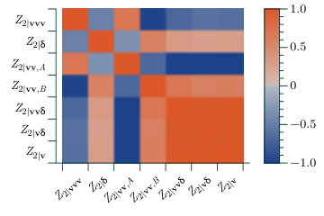
4 Conclusions

In this paper we have presented the complete one-loop renormalization of the redshift-space power spectrum and its Legendre multipoles $\ell=0$ , $\ell=2$ and $\ell=4$ . The same principles apply to modes with $\ell\geqslant 6$ , but our numerical results for the hexadecapole are already noisy and present-day observational constraints on this multipole are not yet competitive with the monopole or quadrupole.

The outcome of a similar renormalization has already been reported by Lewandowski et al. [18] in an approximation where all growth functions are replaced by their Einstein–de Sitter counterparts. In this paper we include the exact time dependence for the first time, showing that—at least within the EFT framework, although not for SPT—it is an excellent approximation for the real-space power spectrum and $\ell=0$ mode, but leads to $\sim 2\%$ errors in the $\ell=2,4$ modes for $k\gtrsim 0.1h/\text{Mpc}$ . Results including exact time dependence were given in Refs. [10, 25], and applied to redshift space in models more general than $\Lambda$ CDM by Fasiello & Vlah [24]. However, because they did not commit to a specific scenario they quoted their results as unevaluated quadratures. The explicit time dependence of the SPT redshift-space power spectrum is a new result.

Comparison with previous results.—Our formalism is broadly in agreement with the methods used in Refs. [14, 18, 19]. In our presentation we have emphasized the role of the counterterms in parametrizing ultraviolet contributions to loop integrals, rather than arising from smoothed equations of motion. The resulting language is closer to familiar applications of effective field theory in particle physics. In addition, our formalism differs from that presented by Lewandowski et al. [18] in certain technical details, and in our procedure to fit for the counterterms of the redshift-space power spectrum.

For a cosmology matching the MultiDark MDR1 simulation, we find that the real-space power spectrum and the $\ell=0$ mode of the redshift-space power spectrum can be matched within $\sim 5\%$ using the leading EFT counterterm up to roughly $k\lesssim 0.4h/\text{Mpc}$ at $z=0$ , and with a firm upper limit of $k\lesssim 0.74h/\text{Mpc}$ that follows from imposing positivity of the $\ell=0$ mode. In practice the higher-order counterterms that restore positivity are presumably already important at substantially smaller wavenumbers.

These maximum $k$ -values are somewhat larger than those found by Lewandowski et al., who reported a fit with $<2\%$ error to a redshift-space power spectrum extracted from the BigMDPL simulation up to $k\lesssim 0.13h/\text{Mpc}$ at $z=0.56$ . At this redshift, they estimated that higher-order counterterms might already be important at $k=0.2h/\text{Mpc}$ , and suggested that the non-linear scale that controls breakdown of the EFT expansion might sit near $k\approx 0.8h/\text{Mpc}$ . Our results are more comparable to those reported by Perko et al., who worked with the halo power spectrum and found a good match up to $k=0.43h/\text{Mpc}$ at $z=0.67$ . Their fit included more counterterms (roughly, four bias parameters and three stochastic counterterms) and therefore the degree to which our predictions can be compared is not entirely clear. Nevertheless, the qualitative features are very similar.

Our results could also be compared with the ‘improved’ perturbation theory of Taruya, Nishimichi & Saito [64]. Their prediction can be written as a suppressed Kaiser power spectrum with corrections,

P_{s}=D_{\text{FoG}}(k\mu f\sigma_{\text{v}})\Big(P_{\delta\delta}+2f\mu^{2}P_{\delta\theta}+f^{2}\mu^{4}P_{\theta\theta}\Big)+A(k,\mu)+B(k,\mu),

(105)

where $D_{\text{FoG}}$ is a fingers-of-God suppression factor to be chosen by hand, and $A(k,\mu)$ and $B(k,\mu)$ represent a subset of the terms generated by the composite operators $\bm{\mathrm{{v}}}\delta$ , $\bm{\mathrm{{v}}}\bm{\mathrm{{v}}}$ , $\bm{\mathrm{{v}}}\bm{\mathrm{{v}}}\delta$ and $\bm{\mathrm{{v}}}\bm{\mathrm{{v}}}\bm{\mathrm{{v}}}$ in (60). If the power spectra $P_{\delta\delta}$ , $P_{\delta\theta}$ and $P_{\theta\theta}$ are evaluated at one-loop and we take $D_{\text{FoG}}\approx\exp(-k^{2}\mu^{2}f^{2}\sigma_{\text{v}}^{2})\approx 1-k^{2}\mu^{2}f^{2}\sigma_{\text{v}}^{2}$ , then this very nearly reproduces Matsubara’s SPT result for $P_{s}$ [64]. Instead, Taruya et al. obtained their improvement by evaluating the power spectra using an alternative prescription [101, 102]. By comparing this model to $N$ -body simulations they were able to demonstrate $\sim 1\%$ accuracy up to $k\lesssim 0.2h/\text{Mpc}$ for the monopole and quadrupole at $z=0.5$ . This model is intended to capture physical effects similar to those used in the EFT model, but these effects appear in different ways: subtraction of power for quasilinear $k$ from $D_{\text{FoG}}$ rather than counterterms, and damping of the acoustic oscillations from a combination of $D_{\text{FoG}}$ and the modified computation of $P_{\delta\delta}$ , $P_{\delta\theta}$ , $P_{\theta\theta}$ rather than resummation. The final predictions are broadly comparable, and it would be interesting to understand more clearly how these descriptions are related.

Outlook.—Although we cannot rely on perturbation theory to determine the time-dependence of the counterterms, we show that independent fits for their values at $z\in\{0,0.25,0.5,0.75,1\}$ are compatible with the time-dependence predicted by the perturbative expansion. In addition, as part of our calculation we have introduced a number of technical innovations:

•

We use a new method to decompose the tensor integrals that appear in $P_{s}$ at one-loop level (§3.2), and use it to extract their $\mu$ -dependence. This method is based on the Rayleigh plane-wave expansion and analytic integrals over two or three spherical Bessel functions.
•

We have extended the resummation scheme proposed by Vlah, Seljak, Chu & Feng [16] to redshift space (§3.3). This simplifies calculation of the resummed $P_{\ell}$ by comparison with the resummation scheme suggested by Senatore & Zaldarriaga [13].

In redshift-space this and similar schemes appear similar to the suppression factors used phenomenologically to model the fingers-of-God effect. However we argue that it is more appropriate to interpret the redshift-space counterterms as the source of this suppression, which arises (at least in part) from virialized motions on small scales [39]. Specifically, we show that the redshift-space EFT counterterms successfully reproduce the zero-crossing of the $\ell=2$ mode, which is associated with this suppression.

We find that the effective field-theory framework successfully produces fits that extend the reach of perturbation theory by a factor of a few in $k$ . While this is a considerable achievement, the practical value of these fitting functions has not yet been demonstrated. First, without a prediction for the time-dependence of the counterterms we are obliged to fit independently at each redshift. This reduces the predictivity of the formalism. Second, the values of the counterterms vary even between relatively nearby cosmologies such as the Planck2015 and MDR1 models studied in this paper. A proposal to evade the requirement to renormalize on a model-by-model basis has been given by Cantaneo, Foreman & Senatore [99]. In cases where this or a similar method can be used, the EFT method may be advantageous for parameter fitting or Fisher forecasts. Specifically, we can reduce the computational requirements if it is possible to produce high-precision predictions over a region of parameter space using sparser coverage with $N$ -body simulations than if we were to achieve the same precision by interpolating the power spectra from these simulations directly.

An alternative use case is to compute covariance matrices that extend to small scales, as suggested by Bertolini et al. [103] and Mohammed, Seljak & Vlah [104]. Our results suggest that accurately modelling redshift-space measurements gives enhanced value to both these use cases. As explained in §3.5, we find that bulk flows converge very slowly and exhibit large sample variance, while small-scale velocity effects give important contributions to the redshift-space power spectrum on larger scales. This requirement for high-resolution simulations in large volumes implies that numerical estimation of redshift-space measurements is substantially more expensive than simulation of real-space measurements at the same accuracy. If EFT methods can be used to mitigate this expense then their deployment becomes even more attractive.

Acknowledgements.

The work reported in this paper has been supported by the European Research Council under the European Union’s Seventh Framework Programme (FP/2007–2013) and ERC Grant Agreement No. 308082 (DR, DS). LFdlB acknowledges support from the UK Science and Technology Facilities Council via Research Training Grant ST/M503836/1. Data availability statement.—Computation of the 1-loop matter power spectrum and its multipole decomposition was performed by computer codes, as described in Appendix C. These codes are available for download under open-source licenses. The specific datasets used to construct the EFT power spectra reported in §2.6 and §3.6 have been made available at zenodo.org. This deposit also includes the CAMB parameter files used to construct the linear power spectra, and settings files needed for gevolution to perform the

N

-body simulations described in §3.5. Digital identifiers, attribution information, and licensing conditions are listed in Appendix C for each of these products.

Appendix A Resummation using the Senatore–Zaldarriaga procedure

In §2.5 we described the resummation method of Vlah, Seljak, Chu & Feng (the ‘VSCF scheme’), which makes explicit use of a decomposition into ‘wiggle’ and ‘no-wiggle’ components. This decomposition was critical in allowing the formal Lagrangian-theory expression (44) to be rewritten in terms of $P^{\leqslant{1}\ell}_{\text{w}}$ and $P^{\leqslant{1}\ell}_{\text{nw}}$ even when the exponential is not completely expanded. Without this step it would not have been possible to extract a simple, analytic resummation ‘template’.

Senatore & Zaldarriaga suggested a different resummation prescription that does not make explicit use of this decomposition [13, 14]. Therefore the relation between these schemes is not completely clear. In this Appendix we briefly sketch the Senatore–Zaldarriaga procedure and explain how it is related to the method of Vlah, Seljak, Chu & Feng.

Isolate infrared contributions.—We define $K(\bm{\mathrm{{q}}},\bm{\mathrm{{k}}})$ to be the exponential kernel in the Lagrangian formula for the power spectrum,

K(\bm{\mathrm{{q}}},\bm{\mathrm{{k}}})\equiv\exp\bigg({-\frac{1}{2}}k_{i}k_{j}A_{ij}+\frac{\mathrm{i}}{6}k_{i}k_{j}k_{\ell}W_{ij\ell}+\cdots\bigg).

(106)

The main strategy in the VSCF scheme is to separate the ‘no-wiggle’ component of $K$ from the remainder; cf. (49). Senatore & Zaldarriaga instead chose to isolate the infrared contribution from the two-point function $A_{ij}$ . This yields a new kernel $K_{\text{IR}}$ that satisfies

K_{\text{IR}}(\bm{\mathrm{{q}}},\bm{\mathrm{{k}}})\approx\exp\bigg({-\frac{1}{2}}k_{i}k_{j}A^{\text{IR}}_{ij}\bigg),

(107)

where $A^{\text{IR}}_{ij}$ continues to be defined by (45a), but with the form-factors $X$ and $Y$ in Eqs. (46a)–(46b) evaluated at tree-level and restricted to wavenumbers in the infrared. Then the power spectrum (44) can be written

P(k)=\int\mathrm{d}^{3}q\;\mathrm{e}^{{-\mathrm{i}\bm{\mathrm{{q}}}\cdot\bm{\mathrm{{k}}}}}\Big[K_{\text{IR}}(\bm{\mathrm{{q}}},\bm{\mathrm{{k}}})\Big]\Big[K_{\text{IR}}^{-1}(\bm{\mathrm{{q}}},\bm{\mathrm{{k}}})K(\bm{\mathrm{{q}}},\bm{\mathrm{{k}}})\Big].

(108)

Notice that both factors in square brackets $[\cdots]$ contain ‘wiggle‘ and ‘no-wiggle’ contributions, although the ‘wiggle’ terms in $K_{\text{IR}}$ will be very small and could be dropped.

If all quantities were expanded to one-loop then this expression must reproduce the one-loop Eulerian power spectrum. Therefore the infrared-subtracted kernel $K_{\text{IR}}^{-1}K$ by itself can differ from the one-loop Eulerian result only by terms that involve $A^{\text{IR}}_{ij}$ ,

\int\mathrm{d}^{3}q\;\mathrm{e}^{{-\mathrm{i}\bm{\mathrm{{q}}}\cdot\bm{\mathrm{{k}}}}}\Big[K_{\text{IR}}^{-1}(\bm{\mathrm{{q}}},\bm{\mathrm{{k}}})K(\bm{\mathrm{{q}}},\bm{\mathrm{{k}}})\Big]\approx P^{\leqslant{1}\ell}(k)-\Pi_{\text{IR}}(k),

(109)

where $\Pi_{\text{IR}}$ is defined by

\Pi_{\text{IR}}(k)=P^{={0}\ell}_{\text{IR}}(k)+\frac{1}{4}\int\mathrm{d}^{3}q\;\mathrm{e}^{{-\mathrm{i}\bm{\mathrm{{q}}}\cdot\bm{\mathrm{{k}}}}}\,k_{i}k_{j}k_{m}k_{n}A^{\text{IR}}_{ij}(\bm{\mathrm{{q}}})\Big(A_{mn}^{={0}\ell}(\bm{\mathrm{{q}}})-A^{\text{IR}}_{mn}(\bm{\mathrm{{q}}})\Big).

(110)

This correction subtracts some of the power in $P^{\leqslant{1}\ell}$ arising from infrared modes. To rewrite the factor $K_{\text{IR}}^{-1}K$ in (108) using this result, insert a decomposition of unity in the form

1\equiv\int\mathrm{d}^{3}q^{\prime}\;\delta_{\text{D}}(\bm{\mathrm{{q}}}-\bm{\mathrm{{q}}}^{\prime})\equiv\int\frac{\mathrm{d}^{3}q^{\prime}\,\mathrm{d}^{3}k^{\prime}}{(2\pi)^{3}}\mathrm{e}^{{\mathrm{i}\bm{\mathrm{{k}}}^{\prime}\cdot(\bm{\mathrm{{q}}}-\bm{\mathrm{{q}}}^{\prime})}},

(111)

where $\delta_{\text{D}}$ is the Dirac $\delta$ -function. This yields

P(k)=\int\mathrm{d}^{3}q\int\mathrm{d}^{3}q^{\prime}\int\frac{\mathrm{d}^{3}k^{\prime}}{(2\pi)^{3}}\mathrm{e}^{{-\mathrm{i}\bm{\mathrm{{q}}}\cdot(\bm{\mathrm{{k}}}-\bm{\mathrm{{k}}}^{\prime})}}\mathrm{e}^{{-\mathrm{i}\bm{\mathrm{{k}}}^{\prime}\cdot\bm{\mathrm{{q}}}^{\prime}}}K_{\text{IR}}(\bm{\mathrm{{q}}},\bm{\mathrm{{k}}})\Big[K_{\text{IR}}^{-1}(\bm{\mathrm{{q}}}^{\prime},\bm{\mathrm{{k}}})K(\bm{\mathrm{{q}}}^{\prime},\bm{\mathrm{{k}}})\Big].

(112)

Integrate $K_{\text{IR}}$ to a smoothing kernel.—If $K_{\text{IR}}$ depends only weakly on $\bm{\mathrm{{q}}}$ then the integral over $\mathrm{d}^{3}q$ produces a kernel that has support only in a narrow region where $\bm{\mathrm{{k}}}\approx\bm{\mathrm{{k}}}^{\prime}$ . This relation becomes exact in the limit that $K_{\text{IR}}$ has no dependence on $\bm{\mathrm{{q}}}$ . Although this is not the case it practice, it gives a simple scenario in which to visualize the outcome of the integration. The kernel is proportional to $\delta_{\text{D}}(\bm{\mathrm{{k}}}-\bm{\mathrm{{k}}}^{\prime})$ if $K_{\text{IR}}$ also has no dependence on $\bm{\mathrm{{k}}}$ , and convolution with it has no effect. Otherwise, the kernel can be expanded as a series in derivatives of $\delta_{\text{D}}(\bm{\mathrm{{k}}}-\bm{\mathrm{{k}}}^{\prime})$ , and convolution with it represents a local smoothing. For (107), the shape of the smoothing kernel is determined by the Gaussian $k$ -dependence of $K_{\text{IR}}$ , and the width of its smoothing window is determined by the amplitude of $X$ and $Y$ .

Returning finally to the case where $X$ , $Y$ and $K_{\text{IR}}$ have weak $\bm{\mathrm{{q}}}$ -dependence, we can make a Taylor expansion in $\bm{\mathrm{{q}}}$ around some fiducial value and exchange explicit powers of $\bm{\mathrm{{q}}}$ for further derivatives with respect to $\bm{\mathrm{{k}}}$ or $\bm{\mathrm{{k}}}^{\prime}$ . Therefore each term in the series expansion integrates to an increasingly high-derivative smoothing kernel. The result can be regarded as a superposition of smoothing kernels with varying widths determined by the variation of $X$ and $Y$ with $\bm{\mathrm{{q}}}$ . Therefore the smoothing is modulated on the scale of the infrared modes retained in these form-factors. This modulation partially restores the infrared power subtracted by $\Pi_{\text{IR}}$ .

These arguments are strictly valid only when it is safe to commute limits and summations with the integration over $\bm{\mathrm{{q}}}$ . Assuming such exchanges to be acceptable, however, we can collect all these together to obtain a net smoothing kernel $M(\bm{\mathrm{{k}}},\bm{\mathrm{{k}}}^{\prime})$ defined by

M(\bm{\mathrm{{k}}},\bm{\mathrm{{k}}}^{\prime})=\int\mathrm{d}^{3}q\,\mathrm{e}^{{-\mathrm{i}\bm{\mathrm{{q}}}\cdot(\bm{\mathrm{{k}}}-\bm{\mathrm{{k}}}^{\prime})}}K_{\text{IR}}(\bm{\mathrm{{q}}},\bm{\mathrm{{k}}}).

(113)

Resummed template is smoothed power spectrum.—The final step is to use the approximation that $M(\bm{\mathrm{{k}}},\bm{\mathrm{{k}}}^{\prime})$ has support only near $\bm{\mathrm{{k}}}\approx\bm{\mathrm{{k}}}^{\prime}$ to exchange the $\bm{\mathrm{{k}}}$ -dependence of $K_{\text{IR}}^{-1}K$ for $\bm{\mathrm{{k}}}^{\prime}$ -dependence. The effect is to average $\mathrm{e}^{{\mathrm{i}\bm{\mathrm{{k}}}^{\prime}\cdot\bm{\mathrm{{q}}}^{\prime}}}K_{\text{IR}}^{-1}(\bm{\mathrm{{q}}}^{\prime},\bm{\mathrm{{k}}}^{\prime})K(\bm{\mathrm{{q}}}^{\prime},\bm{\mathrm{{k}}}^{\prime})$ over a range of $\bm{\mathrm{{k}}}^{\prime}$ near $\bm{\mathrm{{k}}}$ . The error in this approximation comes from the inclusion of $\mathrm{e}^{{\mathrm{i}\bm{\mathrm{{k}}}^{\prime}\cdot\bm{\mathrm{{q}}}^{\prime}}}$ in the average, and can be expressed in terms of gradients of the smoothing kernel in $\bm{\mathrm{{k}}}$ . If the smoothing does not vary rapidly with wavenumber we may hope it is not large. Proceeding in this way, Senatore & Zaldarriaga obtained the template [13, 18]

P_{\text{SZ}}(k)=\int\frac{\mathrm{d}^{3}k^{\prime}}{(2\pi)^{3}}M(\bm{\mathrm{{k}}},\bm{\mathrm{{k}}}^{\prime})\left[P^{\leqslant{1}\ell}(k^{\prime})-\Pi_{\text{IR}}(k^{\prime})\right].

(114)

If the power spectrum is nearly constant in $k$ then it is unaffected by the smoothing kernel, and therefore the ‘no-wiggle’ component will be practically unchanged. But the ‘wiggle’ component is averaged, causing it to be suppressed. Therefore, in the Senatore & Zaldarriaga scheme, the separation into ‘wiggle’ and ‘no-wiggle’ components becomes important only in the final average. However, the net effect is still to suppress the acoustic oscillations while leaving the broadband power unchanged.

Note that in the VSCF scheme the amount of suppression applied to the ‘wiggle’ component at wavenumber $k$ is determined by $k/k_{\text{damp}}$ , where as explained in §2.5 the wavenumber $k_{\text{damp}}$ measures the typical total displacement of particles averaged between $q_{\text{min}}$ and $q_{\text{max}}$ ; the infrared modes are not treated separately. In the Senatore–Zaldarriaga scheme we smooth the power spectrum over a window set by the typical displacement induced by infrared modes only, averaged over all scales. The final resummed power spectra are qualitatively similar, but there is no simple relation between the two procedures.

Although the Senatore–Zaldarriaga scheme is elegant, it has computational drawbacks. When applied to redshift-space distortions it is necessary to treat the angular dependence of the integrals numerically. This significantly increases the computational burden. By comparison, in the VSCF scheme the angular dependence can be extracted analytically [cf. Eqs. (90) and (91)], which simplifies the resummation procedure.

Appendix B Fabrikant’s procedure to evaluate the three-Bessel integrals

In §3.2 we described a new procedure for computing the redshift-space one-loop SPT power spectrum $P_{s}^{\text{SPT}}$ , based on the Rayleigh plane-wave expansion. To reduce the resulting expressions to closed form we must integrate over the Bessel functions appearing in the Rayleigh formula. For 13-type integrals this requires weighted integrals over two Bessel functions, which are relatively well-understood. For 22-type integrals it requires weighted integrals over three Bessel functions. These are substantially more difficult to evaluate.

Context.—In 1936, Bailey gave the formula (for positive $a$ , $b$ and $c$ )

\begin{split}\int_{0}^{\infty}t^{\lambda-1}J_{\mu}(at)J_{\nu}(bt)J_{\rho}(ct)\,\mathrm{d}t=\mbox{}&\frac{2^{\lambda-1}a^{\mu}b^{\nu}\Gamma(\frac{\lambda+\mu+\nu+\rho}{2})}{c^{\lambda+\mu+\nu}\Gamma(\mu+1)\Gamma(\nu+1)\Gamma(1-\frac{\lambda+\mu+\nu+\rho}{2})}\\ &\mbox{}\times F_{4}\bigg(\begin{array}[]{l@{\hspace{2mm}}l@{\hspace{2mm}}l}{[}\lambda+\mu+\nu-\rho{]}/2,\hfil\hskip 5.69054pt&\mu+1,\hfil\hskip 5.69054pt&a^{2}/c^{2}\\ {[}\lambda+\mu+\nu+\rho{]}/2,\hfil\hskip 5.69054pt&\nu+1,\hfil\hskip 5.69054pt&b^{2}/c^{2}\end{array}\bigg),\end{split}

(115)

where $\newRe(\lambda+\mu+\nu+\rho)>0$ , $\newRe(\lambda)<5/2$ , and $c>a+b$ ; the function $F_{4}$ is the fourth type of Appell hypergeometric function,

F_{4}\bigg(\begin{array}[]{l@{\hspace{2mm}}l@{\hspace{2mm}}l}a,\hfil\hskip 5.69054pt&c_{1},\hfil\hskip 5.69054pt&x\\ b,\hfil\hskip 5.69054pt&c_{2},\hfil\hskip 5.69054pt&y\end{array}\bigg)\equiv\sum_{m,n=0}^{\infty}\frac{({a})^{m+n}({b})^{m+n}}{({c_{1}})^{m}({c_{2}})^{n}m!n!}x^{m}y^{n}.

(116)

Here, $({x})^{a}$ is the Pochhammer symbol (or ‘rising factorial’) defined by $({x})^{a}=\Gamma(x+a)/\Gamma(a)$ . The condition $c>a+b$ implies that the lengths $a$ , $b$ , $c$ do not form the sides of a triangle. Bailey’s methods did not determine the integral when this condition is not satisfied. In particular, there is no reason for the result to be analytic in $a$ , $b$ and $c$ and therefore we cannot extend (115) by analytic continuation. (Some results based on analytic continuation are known in special cases; see the discussion in Ref. [27].)

Various extensions of Bailey’s results are known. Fabrikant and Dôme used a different computational technique to find integral representations that could be evaluated explicitly [105, 106], but still in the non-triangular case. Mehrem used the Rayleigh plane-wave expansion (67) to determine various integrals over two and three spherical Bessel functions, again in the non-triangular case and only when a Clebsch–Gordon coefficient involving the orders $\mu$ , $\nu$ , $\sigma$ is not zero [107, 108]. Earlier, Gervois & Navelet [109, 27] had studied the (spherical) three-Bessel integral even in the case where $(a,b,c)$ do form a triangle. Their result appears in its most developed form in Table 2 of Ref. [27], which can be applied whenever $\lambda+\mu+\nu+\rho$ is an integer.

This result of Gervois & Navelet is already sufficient for the purposes of this paper (where $\mu$ , $\nu$ , $\sigma$ and $\lambda$ are individually integers), but in our practical calculations we make use of a more recent formalism due to Fabrikant [28]. The Fabrikant method is equivalent to that of Gervois & Navelet when $\lambda+\mu+\nu+\rho$ is an integer, but is marginally more general because it allows for non-integer $\lambda$ .

Fabrikant’s method.—We briefly summarize the procedure. The aim is to compute a generalization of the integral (71),

I=\int_{0}^{\infty}x^{\lambda}j_{\mu}(kx)j_{\nu}(qx)j_{\sigma}(sx)\,\mathrm{d}x,

(117)

where $\mu$ , $\nu$ and $\sigma$ are integers, and $\lambda$ , $k$ , $q$ , and $s$ are real. Fabrikant rewrote the spherical Bessel functions as derivatives of trigonometric functions,

j_{n}(z)=(-1)^{n}z^{n}\left(\frac{\mathrm{d}}{z\,\mathrm{d}z}\right)^{n}\frac{\sin z}{z},

(118)

which allows $I$ to be expressed in the form

I=(-1)^{\mu+\nu+\sigma}a^{\mu}b^{\nu}c^{\sigma}\frac{\partial^{\mu}}{(a\,\partial a)^{\mu}}\frac{\partial^{\nu}}{(b\,\partial b)^{\nu}}\frac{\partial^{\sigma}}{(c\,\partial c)^{\sigma}}\int_{0}^{\infty}\frac{\sin at\sin bt\sin ct}{abc\,t^{\mu+\nu+\sigma+3-\lambda}}\,\mathrm{d}t.

(119)

The integral in this expression may be formally divergent, but where $I$ exists the differentiation will yield a finite result. It can be performed using standard trigonometric identities, yielding

\begin{split}I=\mbox{}&(-1)^{\mu+\nu+\sigma}a^{\mu}b^{\nu}c^{\sigma}\cos\frac{\pi}{2}(\mu+\nu+\sigma+3-\lambda)\frac{\partial^{\mu}}{(a\,\partial a)^{\mu}}\frac{\partial^{\nu}}{(b\,\partial b)^{\nu}}\frac{\partial^{\sigma}}{(c\,\partial c)^{\sigma}}\frac{\Gamma(\lambda-\mu-\nu-\sigma-2)}{4abc}\\ &\mbox{}\times\bigg(|c+a-b|^{\mu+\nu+\sigma+2-\lambda}\sgn(c+a-b)+\text{2 cyclic perms}-(a+b+c)^{\mu+\nu+\sigma+2-\lambda}\bigg)\end{split}

(120)

where $\sgn(x)$ is the sign function, defined by $\sgn(x)=x/|x|$ for $x\neq 0$ and $\sgn(0)=0$ . Compare Eq. (120) with Eqs. (3.8), (3.9) and (3.10) of Ref. [27].

If the argument of the $\cos$ or $\Gamma$ functions is zero, then the result should be computed via a limit. The differentiations can be performed using Mathematica, or by using the formula

z^{n+1}\frac{\partial^{n+1}f(z)}{(z\,\partial z)^{n+1}}=\sum_{k=0}^{\lfloor n/2\rfloor}\frac{\Gamma(n+2k+1)f^{(n-2k+1)}(z)}{\Gamma(2k+1)\Gamma(n-2k+1)(2z)^{2k}}-\sum_{k=0}^{\lfloor(n-1)/2\rfloor}\frac{\Gamma(n+2k+2)f^{(n-2k)}(z)}{\Gamma(2k+2)\Gamma(n-2k)(2z)^{2k+1}}.

(121)

The quantity $\lfloor x\rfloor$ is the floor of $x$ , ie. the largest integer that does not exceed $x$ , and $f^{(n)}(x)$ is the $n^{\text{th}}$ derivative of $f$ . As part of the software bundle accompanying this paper we provide a Mathematica notebook to evaluate Eqs. (120) and (121). It will automatically test the resulting expression against results obtained using Mathematica’s built-in integration strategies for highly oscillatory integrals.

Specific results.—We collect the results needed for the computation of $P_{s}^{\text{SPT}}$ .


$\displaystyle\mathscr{J}^{0}_{{0}{0}}$	$\displaystyle=\frac{\pi}{4kqs}$	(122a)
$\displaystyle\mathscr{J}^{1}_{{1}{0}}$	$\displaystyle=\frac{\pi}{8}\frac{k^{2}+q^{2}-s^{2}}{k^{2}q^{2}s}$	(122b)
$\displaystyle\mathscr{J}^{2}_{{2}{0}}$	$\displaystyle=\frac{\pi}{32}\frac{3k^{4}+2k^{2}(q^{2}-3s^{2})+3(q^{2}-s^{2})^{2}}{k^{3}q^{3}s}$	(122c)
$\displaystyle\mathscr{J}^{2}_{{2}{2}}$	$\displaystyle=\frac{\pi}{64}\frac{(3k^{4}+2k^{2}q^{2}+3q^{4})s^{2}+3(k^{2}+q^{2})s^{4}-3(k^{2}-q^{2})^{2}(k^{2}+q^{2})-3s^{6}}{k^{3}q^{3}s^{3}}$	(122d)
$\displaystyle\mathscr{J}^{2}_{{3}{1}}$	$\displaystyle=\frac{\pi}{64}\frac{3k^{4}(q^{2}+5s^{2})+(q^{2}-s^{2})^{2}(q^{2}+5s^{2})+k^{2}(q^{4}+6q^{2}s^{2}-15s^{4})-5k^{6}}{k^{3}q^{4}s^{2}}$	(122e)
$\displaystyle\mathscr{J}^{2}_{{4}{2}}$	$\displaystyle=\frac{\pi}{512}\frac{1}{k^{3}q^{5}s^{3}}\Big(35k^{8}-20k^{6}(3q^{2}+7s^{2})+6k^{4}(3q^{4}+10q^{2}s^{2}+35s^{2})$
	$\displaystyle\hskip 18.49988pt\hskip 18.49988pt\mbox{}+(q^{2}-s^{2})^{2}(3q^{4}+10q^{2}s^{2}+35s^{4})+4k^{2}(q^{6}+3q^{4}s^{2}+15q^{2}s^{4}-35s^{6})\Big)$	(122f)
$\displaystyle\mathscr{J}^{3}_{{3}{0}}$	$\displaystyle=\frac{\pi}{64}\frac{(k^{2}+q^{2}-s^{2})\big[5k^{4}+5(q^{2}-s^{2})^{2}-2k^{2}(q^{2}+5s^{2})\big]}{k^{4}q^{4}s}$	(122g)
$\displaystyle\mathscr{J}^{4}_{{4}{0}}$	$\displaystyle=\frac{\pi}{512}\frac{1}{k^{4}q^{5}s}\Big(35k^{8}+20k^{2}(q^{2}-7s^{2})\big[k^{4}+(q^{2}-s^{2})^{2}\big]+35(q^{2}-s^{2})^{4}$
	$\displaystyle\hskip 18.49988pt\hskip 18.49988pt\mbox{}+6k^{4}(3q^{4}-30q^{2}s^{2}+35s^{4})\Big)$	(122h)

Index permutations can be obtained by making suitable exchanges of $k$ , $q$ and $s$ ; for example, $\mathscr{J}^{2}_{{1}{3}}$ can be obtained from (122e) by exchanging $q$ and $s$ , and $\mathscr{J}^{0}_{{3}{3}}$ can be obtained from (122g) by exchanging $k$ and $s$ .

Appendix C Accompanying software bundle

The calculations needed to obtain the redshift-space power spectrum are complex. To assist those wishing to replicate our results we have made available a large collection of resources, including Mathematica notebooks that summarize (and validate) the calculation of $\langle\delta_{s}\delta_{s}\rangle$ in SPT, and software tools to compute the loop integrals needed for numerical evaluation.

C.1 Mathematica notebooks

This deposit contains two Mathematica notebooks:

•

FabrikantIntegrals.nb
This notebook implements Fabrikant’s method for evaluation of the three-Bessel integrals, as described in Appendix B. It will automatically test the resulting analytic formulae against numerical results obtained using Mathematica’s built-in integration strategies.
•

SPTPowerSpectrum.nb
This notebook summarizes our analytic calculation of the redshift-space power spectrum up to one-loop. It also validates the result against Matsubara’s result for the redshift-space power spectrum using the Einstein–de Sitter approximation [26], and with the formulae for the velocity power spectrum given by Makino et al. [7].

C.2 One-loop SPT integrals in redshift space

C.2.1 Pipeline A

This is a C++ pipeline for computation of the growth factors and loop integrals needed to construct the renormalized redshift-space power spectrum and its multipoles. It implements the Vlah et al. resummation scheme described in §§2.5 and 3.3.

The implementation is parallelized using MPI and uses adaptive load balancing to spread work over available cores. The Cuba library is used to perform the multidimensional integrations that are required [110], and the SPLINTER library is used to construct B-splines [111]. Results are stored as SQLite databases. The counterterm fits are performed using the CosmoSIS parameter-estimation framework and the emcee sampler, for which a Python module is supplied [112]. The power spectra presented in this paper were computed using git revision 977e5b03.

This pipeline shares some code with the CppTransport platform for computing correlation functions of inflationary density perturbations [113].

C.2.2 Pipeline B

This is a second, independent pipeline that duplicates the functionality of pipeline A, but with slightly different implementation choices. The multidimensional integrations and splines are evaluated using the GNU Scientific Library [114]. The results presented in this paper have been computed using both pipelines A and B, and a third C pipeline implemented using Mathematica. The plots and numerical results are those belonging to pipeline A. The pipeline B results were obtained using git revision 1126b040. We find very good agreement between all pipelines, indicating that our numerics are robust to changes in integration strategy, filtering methods and the counterterm fitting procedure.

C.3 Supporting dataset

This dataset includes the components necessary to reproduce our numerical results. It comprises:

•

SQLite databases containing the output of the pipeline described in C.2.1 for the Planck2015 [38] and MultiDark MDR1 cosmologies [94]. These were used to construct the renormalized real-space power spectrum in §2 and the redshift-space power spectrum in §3, respectively.
•

A settings file for the gevolution numerical relativity code, which was used to perform the custom $N$ -body simulations described in §3.5. Our results used version 1.1 of the gevolution framework. The initial conditions are generated dynamically from the settings file.
•

CAMB parameter files for the linear power spectra used to construct our one-loop results, for both the Planck2015 and MDR1 cosmologies. For the Planck2015 model we also include a CAMB parameter file to compute the final non-linear power spectrum using HALOFIT. These power spectra are also emebedded in the SQLite databases containing our numerical results.

References

(1) R. Juszkiewicz, On the evolution of cosmological adiabatic perturbations in the weakly non-linear regime, Mon. Not. Roy. Astron. Soc. 197 (1981) 931–940.
(2) E. T. Vishniac, Why weakly non-linear effects are small in a zero-pressure cosmology, Mon. Not. Roy. Astron. Soc. 203 (1983) 345–349.
(3) J. N. Fry, The Galaxy correlation hierarchy in perturbation theory, Astrophys. J. 279 (1984) 499–510.
(4) M. H. Goroff, B. Grinstein, S. J. Rey, and M. B. Wise, Coupling of Modes of Cosmological Mass Density Fluctuations, Astrophys. J. 311 (1986) 6–14.
(5) E. Bertschinger and B. Jain, Gravitational instability of cold matter, Astrophys. J. 431 (1994) 486, [astro-ph/9307033].
(6) Y. Suto and M. Sasaki, Quasi nonlinear theory of cosmological selfgravitating systems, Phys. Rev. Lett. 66 (1991) 264–267.
(7) N. Makino, M. Sasaki, and Y. Suto, Analytic approach to the perturbative expansion of nonlinear gravitational fluctuations in cosmological density and velocity fields, Phys. Rev. D46 (1992) 585–602.
(8) F. Bernardeau, S. Colombi, E. Gaztanaga, and R. Scoccimarro, Large scale structure of the universe and cosmological perturbation theory, Phys. Rept. 367 (2002) 1–248, [astro-ph/0112551].
(9) D. Baumann, A. Nicolis, L. Senatore, and M. Zaldarriaga, Cosmological Non-Linearities as an Effective Fluid, JCAP 1207 (2012) 051, [1004.2488].
(10) J. J. M. Carrasco, M. P. Hertzberg, and L. Senatore, The Effective Field Theory of Cosmological Large Scale Structures, JHEP 09 (2012) 082, [1206.2926].
(11) J. J. M. Carrasco, S. Foreman, D. Green, and L. Senatore, The Effective Field Theory of Large Scale Structures at Two Loops, JCAP 1407 (2014) 057, [1310.0464].
(12) R. A. Porto, L. Senatore, and M. Zaldarriaga, The Lagrangian-space Effective Field Theory of Large Scale Structures, JCAP 1405 (2014) 022, [1311.2168].
(13) L. Senatore and M. Zaldarriaga, The IR-resummed Effective Field Theory of Large Scale Structures, JCAP 1502 (2015), no. 02 013, [1404.5954].
(14) L. Senatore and M. Zaldarriaga, Redshift Space Distortions in the Effective Field Theory of Large Scale Structures, 1409.1225.
(15) Z. Vlah, M. White, and A. Aviles, A Lagrangian effective field theory, JCAP 1509 (2015), no. 09 014, [1506.05264].
(16) Z. Vlah, U. Seljak, M. Y. Chu, and Y. Feng, Perturbation theory, effective field theory, and oscillations in the power spectrum, JCAP 1603 (2016), no. 03 057, [1509.02120].
(17) J. C. Jackson, Fingers of God: A critique of Rees’ theory of primoridal gravitational radiation, Mon. Not. Roy. Astron. Soc. 156 (1972) 1P–5P, [0810.3908].
(18) M. Lewandowski, L. Senatore, F. Prada, C. Zhao, and C.-H. Chuang, On the EFT of Large Scale Structures in Redshift Space, 1512.06831.
(19) A. Perko, L. Senatore, E. Jennings, and R. H. Wechsler, Biased Tracers in Redshift Space in the EFT of Large-Scale Structure, 1610.09321.
(20) V. Assassi, D. Baumann, D. Green, and M. Zaldarriaga, Renormalized Halo Bias, JCAP 1408 (2014) 056, [1402.5916].
(21) Gleyzes, Jérôme and de Putter, Roland and Green, Daniel and Doré, Olivier, Biasing and the search for primordial non-Gaussianity beyond the local type, 1612.06366.
(22) B. Bose and K. Koyama, A Perturbative Approach to the Redshift Space Power Spectrum: Beyond the Standard Model, JCAP 1608 (2016), no. 08 032, [1606.02520].
(23) B. Bose and K. Koyama, A Perturbative Approach to the Redshift Space Correlation Function: Beyond the Standard Model, JCAP 1708 (2017), no. 08 029, [1705.09181].
(24) M. Fasiello and Z. Vlah, Nonlinear fields in generalized cosmologies, Phys. Rev. D94 (2016), no. 6 063516, [1604.04612].
(25) M. Lewandowski and L. Senatore, IR-safe and UV-safe integrands in the EFTofLSS with exact time dependence, 1701.07012.
(26) T. Matsubara, Resumming Cosmological Perturbations via the Lagrangian Picture: One-loop Results in Real Space and in Redshift Space, Phys. Rev. D77 (2008) 063530, [0711.2521].
(27) A. Gervois and H. Navelet, Infinite integrals involving three spherical Bessel functions, SIAM Journal on Mathematical Analysis 20 (1989), no. 4 1006–1018, [http://dx.doi.org/10.1137/0520067].
(28) V. Fabrikant, Elementary exact evaluation of infinite integrals of the product of several spherical Bessel functions, power and exponential, Quarterly of Applied Mathematics 71 (2013), no. 3 573–581.
(29) W. N. Bailey, Some infinite integrals involving Bessel functions, Proceedings of the London Mathematical Society s2-40 (1936), no. 1 37–48.
(30) L. Mercolli and E. Pajer, On the velocity in the Effective Field Theory of Large Scale Structures, JCAP 1403 (2014) 006, [1307.3220].
(31) P. Mészáros, The behaviour of point masses in an expanding cosmological substratum, Astron. Astrophys. 37 (1974) 225–228.
(32) E. J. Groth and P. J. E. Peebles, Closed-form solutions for the evolution of density perturbations in some cosmological models, Astron. Astrophys. 41 (June, 1975) 143–145.
(33) E. V. Linder, Cosmic growth history and expansion history, Phys. Rev. D72 (2005) 043529, [astro-ph/0507263].
(34) R. Scoccimarro, S. Colombi, J. N. Fry, J. A. Frieman, E. Hivon, and A. Melott, Nonlinear evolution of the bispectrum of cosmological perturbations, Astrophys. J. 496 (1998) 586, [astro-ph/9704075].
(35) M. B. Wise, Non-Gaussian Fluctuations, NATO Sci. Ser. C. 219 (1988) 215–238.
(36) R. Scoccimarro and J. Frieman, Loop corrections in nonlinear cosmological perturbation theory, Astrophys. J. Suppl. 105 (1996) 37, [astro-ph/9509047].
(37) R. Scoccimarro and J. Frieman, Loop corrections in nonlinear cosmological perturbation theory 2. Two point statistics and selfsimilarity, Astrophys. J. 473 (1996) 620, [astro-ph/9602070].
(38) Planck Collaboration, P. A. R. Ade et al., Planck 2015 results. XIII. Cosmological parameters, Astron. Astrophys. 594 (2016) A13, [1502.01589].
(39) R. Scoccimarro, Redshift-space distortions, pairwise velocities and nonlinearities, Phys. Rev. D70 (2004) 083007, [astro-ph/0407214].
(40) N. S. Sugiyama and D. N. Spergel, How does non-linear dynamics affect the baryon acoustic oscillation?, JCAP 1402 (2014) 042, [1306.6660].
(41) E. Pajer and M. Zaldarriaga, On the Renormalization of the Effective Field Theory of Large Scale Structures, JCAP 1308 (2013) 037, [1301.7182].
(42) J. J. M. Carrasco, S. Foreman, D. Green, and L. Senatore, The 2-loop matter power spectrum and the IR-safe integrand, JCAP 1407 (2014) 056, [1304.4946].
(43) J. F. Donoghue, General relativity as an effective field theory: The leading quantum corrections, Phys. Rev. D50 (1994) 3874–3888, [gr-qc/9405057].
(44) J. F. Donoghue, Introduction to the effective field theory description of gravity, in Advanced School on Effective Theories Almunecar, Spain, June 25-July 1, 1995, 1995. gr-qc/9512024.
(45) P. J. E. Peebles, The Effect of a Lumpy Matter Distribution on the Growth of Irregularities in an Expanding Universe, Astron. Astrophys. 32 (1974) 391.
(46) S. M. Carroll, S. Leichenauer, and J. Pollack, Consistent effective theory of long-wavelength cosmological perturbations, Phys. Rev. D90 (2014), no. 2 023518, [1310.2920].
(47) F. Führer and G. Rigopoulos, Renormalizing a Viscous Fluid Model for Large Scale Structure Formation, JCAP 1602 (2016), no. 02 032, [1509.03073].
(48) R. P. Feynman and F. L. Vernon, Jr., The Theory of a general quantum system interacting with a linear dissipative system, Annals Phys. 24 (1963) 118–173. [Annals Phys.281,547(2000)].
(49) A. O. Caldeira and A. J. Leggett, Influence of dissipation on quantum tunneling in macroscopic systems, Phys. Rev. Lett. 46 (1981) 211.
(50) A. O. Caldeira and A. J. Leggett, Path integral approach to quantum Brownian motion, Physica 121A (1983) 587–616.
(51) A. O. Caldeira and A. J. Leggett, Quantum tunneling in a dissipative system, Annals Phys. 149 (1983) 374–456.
(52) A. Kamenev, Field theory of non-equilibrium systems. Cambridge University Press, 2011.
(53) E. Calzetta and B.-L. Hu, Stochastic behavior of effective field theories across threshold, Phys. Rev. D55 (1997) 3536–3551, [hep-th/9603164].
(54) E. Calzetta and B. L. Hu, Stochastic dynamics of correlations in quantum field theory: From Schwinger-Dyson to Boltzmann-Langevin equation, Phys. Rev. D61 (2000) 025012, [hep-ph/9903291].
(55) C. Itzykson and J. B. Zuber, Quantum Field Theory. International Series In Pure and Applied Physics. McGraw-Hill, New York, 1980.
(56) J. C. Collins, Renormalization, vol. 26 of Cambridge Monographs on Mathematical Physics. Cambridge University Press, Cambridge, 1986.
(57) J. C. Polkinghorne, Models of High Energy Processes. Cambridge Monographs on Mathematical Physics. Cambridge Univ. Press, Cambridge, UK, 2010.
(58) J. R. Bond and H. M. P. Couchman, $w_{gg}({\theta})$ as a probe of large scale structure, in Proceedings of the 2nd Canadian Conference on General Relativity and Relativistic Astrophysics (A. Coley, C. Dyer, and T. Tupper, eds.), pp. 385–389, 1988.
(59) A. N. Taylor, Statistics of self-gravitating fluctuations, in Cosmic Velocity Fields (F. Bouchet and M. Lachieze-Rey, eds.), p. 585, 1993.
(60) A. N. Taylor and A. J. S. Hamilton, Non-linear cosmological power spectra in real and redshift space, Mon. Not. R. Astron. Soc. 282 (Oct., 1996) 767–778, [astro-ph/9604020].
(61) T. Okamura, A. Taruya, and T. Matsubara, Next-to-leading resummation of cosmological perturbations via the Lagrangian picture: 2-loop correction in real and redshift spaces, JCAP 1108 (2011) 012, [1105.1491].
(62) M. McQuinn and M. White, Cosmological perturbation theory in 1+1 dimensions, JCAP 1601 (2016), no. 01 043, [1502.07389].
(63) T. Baldauf, M. Mirbabayi, M. Simonović, and M. Zaldarriaga, Equivalence Principle and the Baryon Acoustic Peak, Phys. Rev. D92 (2015), no. 4 043514, [1504.04366].
(64) A. Taruya, T. Nishimichi, and S. Saito, Baryon Acoustic Oscillations in 2D: Modeling Redshift-space Power Spectrum from Perturbation Theory, Phys. Rev. D82 (2010) 063522, [1006.0699].
(65) D. Blas, M. Garny, M. M. Ivanov, and S. Sibiryakov, Time-Sliced Perturbation Theory II: Baryon Acoustic Oscillations and Infrared Resummation, JCAP 1607 (2016), no. 07 028, [1605.02149].
(66) D. J. Eisenstein and W. Hu, Power spectra for cold dark matter and its variants, Astrophys. J. 511 (1997) 5, [astro-ph/9710252].
(67) D. J. Eisenstein, H.-j. Seo, E. Sirko, and D. Spergel, Improving Cosmological Distance Measurements by Reconstruction of the Baryon Acoustic Peak, Astrophys. J. 664 (2007) 675–679, [astro-ph/0604362].
(68) D. J. Eisenstein, H.-j. Seo, and M. J. White, On the Robustness of the Acoustic Scale in the Low-Redshift Clustering of Matter, Astrophys. J. 664 (2007) 660–674, [astro-ph/0604361].
(69) M. Crocce and R. Scoccimarro, Memory of initial conditions in gravitational clustering, Phys. Rev. D73 (2006) 063520, [astro-ph/0509419].
(70) M. Crocce and R. Scoccimarro, Nonlinear Evolution of Baryon Acoustic Oscillations, Phys. Rev. D77 (2008) 023533, [0704.2783].
(71) VIRGO Consortium Collaboration, R. E. Smith, J. A. Peacock, A. Jenkins, S. D. M. White, C. S. Frenk, F. R. Pearce, P. A. Thomas, G. Efstathiou, and H. M. P. Couchmann, Stable clustering, the halo model and nonlinear cosmological power spectra, Mon. Not. Roy. Astron. Soc. 341 (2003) 1311, [astro-ph/0207664].
(72) R. Takahashi, M. Sato, T. Nishimichi, A. Taruya, and M. Oguri, Revising the Halofit Model for the Nonlinear Matter Power Spectrum, Astrophys. J. 761 (2012) 152, [1208.2701].
(73) E. Jennings, C. M. Baugh, B. Li, G.-B. Zhao, and K. Koyama, Redshift space distortions in f(R) gravity, Mon. Not. Roy. Astron. Soc. 425 (2012) 2128–2143, [1205.2698].
(74) C. Burrage, D. Parkinson, and D. Seery, Beyond the growth rate of cosmic structure: Testing modified gravity models with an extra degree of freedom, 1502.03710.
(75) N. Kaiser, Clustering in real space and in redshift space, Mon. Not. Roy. Astron. Soc. 227 (July, 1987) 1–21.
(76) P. B. Lilje and G. Efstathiou, Gravitationally induced velocity fields in the universe. I – Correlation functions, Mon. Not. Roy. Astron. Soc. 236 (Feb., 1989) 851–864.
(77) C. McGill, The redshift projection. I – Caustics and correlation functions, Mon. Not. Roy. Astron. Soc. 242 (Feb., 1990) 428–438.
(78) S. Cole, K. B. Fisher, and D. H. Weinberg, Fourier analysis of redshift space distortions and the determination of $\Omega$ , Mon. Not. Roy. Astron. Soc. 267 (1994) 785, [astro-ph/9308003].
(79) A. F. Heavens, S. Matarrese, and L. Verde, The Nonlinear redshift-space power spectrum of galaxies, Mon. Not. Roy. Astron. Soc. 301 (1998) 797–808, [astro-ph/9808016].
(80) R. Scoccimarro, H. M. P. Couchman, and J. A. Frieman, The Bispectrum as a Signature of Gravitational Instability in Redshift-Space, Astrophys. J. 517 (1999) 531–540, [astro-ph/9808305].
(81) S. Weinzierl, The Art of computing loop integrals, in Universality and renormalization: From stochastic evolution to renormalization of quantum fields. Proceedings, Workshop on ’Percolation, SLE and related topics’, Toronto, Canada, September 20-24, 2005, and Workshop on ’Renormalization and universality in mathematical physics’, Toronto, Canada, October 18-22, 2005, pp. 345–395, 2006. hep-ph/0604068.
(82) F. E. Neumann, Beiträge zur Theorie der Kugelfuntionen. Leipzig, 1878.
(83) J. C. Adams, On the Expression of the Product of Any Two Legendre’s Coefficients by Means of a Series of Legendre’s Coefficients, Proc. Roy. Soc. 27 (1878).
(84) W. N. Bailey, On the product of two Legendre polynomials, Mathematical Proceedings of the Cambridge Philosophical Society 29 (005, 1933) 173–177.
(85) J. E. McEwen, X. Fang, C. M. Hirata, and J. A. Blazek, FAST-PT: a novel algorithm to calculate convolution integrals in cosmological perturbation theory, JCAP 1609 (2016), no. 09 015, [1603.04826].
(86) X. Fang, J. A. Blazek, J. E. McEwen, and C. M. Hirata, FAST-PT II: an algorithm to calculate convolution integrals of general tensor quantities in cosmological perturbation theory, JCAP 1702 (2017), no. 02 030, [1609.05978].
(87) M. Schmittfull, Z. Vlah, and P. McDonald, Fast large scale structure perturbation theory using one-dimensional fast Fourier transforms, Phys. Rev. D93 (2016), no. 10 103528, [1603.04405].
(88) M. Schmittfull and Z. Vlah, FFT-PT: Reducing the two-loop large-scale structure power spectrum to low-dimensional radial integrals, Phys. Rev. D94 (2016), no. 10 103530, [1609.00349].
(89) J. A. Peacock and S. J. Dodds, Reconstructing the linear power spectrum of cosmological mass fluctuations, Mon. Not. Roy. Astron. Soc. 267 (1994) 1020–1034, [astro-ph/9311057].
(90) K. Yamamoto, T. Sato, and G. Huetsi, Testing general relativity with the multipole spectra of the SDSS luminous red galaxies, Prog. Theor. Phys. 120 (2008) 609–614, [0805.4789].
(91) C. Blake et al., The WiggleZ Dark Energy Survey: the growth rate of cosmic structure since redshift z=0.9, Mon. Not. Roy. Astron. Soc. 415 (2011) 2876, [1104.2948].
(92) A. Oka, S. Saito, T. Nishimichi, A. Taruya, and K. Yamamoto, Simultaneous constraints on the growth of structure and cosmic expansion from the multipole power spectra of the SDSS DR7 LRG sample, Mon. Not. Roy. Astron. Soc. 439 (2014) 2515–2530, [1310.2820].
(93) BOSS Collaboration, F. Beutler et al., The clustering of galaxies in the SDSS-III Baryon Oscillation Spectroscopic Survey: Testing gravity with redshift-space distortions using the power spectrum multipoles, Mon. Not. Roy. Astron. Soc. 443 (2014), no. 2 1065–1089, [1312.4611].
(94) F. Prada, A. A. Klypin, A. J. Cuesta, J. E. Betancort-Rijo, and J. Primack, Halo concentrations in the standard LCDM cosmology, Mon. Not. Roy. Astron. Soc. 423 (2012) 3018–3030, [1104.5130].
(95) J. Adamek, D. Daverio, R. Durrer, and M. Kunz, General relativity and cosmic structure formation, Nature Phys. 12 (2016) 346–349, [1509.01699].
(96) D. Jeong and E. Komatsu, Perturbation Theory Reloaded II: Non-linear Bias, Baryon Acoustic Oscillations and Millennium Simulation In Real Space, Astrophys. J. 691 (2009) 569–595, [0805.2632].
(97) E. Jennings, C. M. Baugh, and S. Pascoli, Modelling redshift space distortions in hierarchical cosmologies, Mon. Not. Roy. Astron. Soc. 410 (Jan., 2011) 2081–2094, [1003.4282].
(98) A. Klypin, G. Yepes, S. Gottlöber, F. Prada, and S. Heß, MultiDark simulations: the story of dark matter halo concentrations and density profiles, Mon. Not. Roy. Astron. Soc. 457 (Apr., 2016) 4340–4359, [1411.4001].
(99) M. Cataneo, S. Foreman, and L. Senatore, Efficient exploration of cosmology dependence in the EFT of LSS, 1606.03633.
(100) M. P. Hertzberg, Effective field theory of dark matter and structure formation: Semianalytical results, Phys. Rev. D89 (2014), no. 4 043521, [1208.0839].
(101) A. Taruya and T. Hiramatsu, A Closure Theory for Non-linear Evolution of Cosmological Power Spectra, Astrophys. J. 674 (2008) 617, [0708.1367].
(102) A. Taruya, T. Nishimichi, S. Saito, and T. Hiramatsu, Non-linear Evolution of Baryon Acoustic Oscillations from Improved Perturbation Theory in Real and Redshift Spaces, Phys. Rev. D80 (2009) 123503, [0906.0507].
(103) D. Bertolini, K. Schutz, M. P. Solon, J. R. Walsh, and K. M. Zurek, Non-Gaussian Covariance of the Matter Power Spectrum in the Effective Field Theory of Large Scale Structure, Phys. Rev. D93 (2016), no. 12 123505, [1512.07630].
(104) I. Mohammed, U. Seljak, and Z. Vlah, Perturbative approach to covariance matrix of the matter power spectrum, Mon. Not. Roy. Astron. Soc. (2016) [1607.00043].
(105) V. Fabrikant and G. Dôme, Elementary evaluation of certain infinite integrals involving Bessel functions, Quarterly of Applied Mathematics 59 (2001), no. 1 1–24.
(106) V. I. Fabrikant, Computation of infinite integrals involving three Bessel functions by introduction of new formalism, ZAMM-Journal of Applied Mathematics and Mechanics/Zeitschrift für Angewandte Mathematik und Mechanik 83 (2003), no. 6 363–374.
(107) R. Mehrem, The plane wave expansion, infinite integrals and identities involving spherical Bessel functions, Applied Mathematics and Computation 217 (2011), no. 12 5360–5365, [0909.0494].
(108) R. Mehrem and A. Hohenegger, A Generalisation For The Infinite Integral Over Three Spherical Bessel Functions, J. Phys. A43 (2010), no. 45 9, [1006.2108].
(109) A. Gervois and H. Navelet, Some integrals involving three Bessel functions when their arguments satisfy the triangle inequalities, Journal of Mathematical Physics 25 (1984), no. 11 3350–3356, [http://dx.doi.org/10.1063/1.526062].
(110) T. Hahn, CUBA: A Library for multidimensional numerical integration, Comput. Phys. Commun. 168 (2005) 78–95, [hep-ph/0404043].
(111) B. Grimstad et al., “SPLINTER: a library for multivariate function approximation with splines.” http://github.com/bgrimstad/splinter, 2015. Accessed: 2016-03-20.
(112) J. Zuntz, M. Paterno, E. Jennings, D. Rudd, A. Manzotti, S. Dodelson, S. Bridle, S. Sehrish, and J. Kowalkowski, CosmoSIS: Modular Cosmological Parameter Estimation, Astron. Comput. 12 (2015) 45–59, [1409.3409].
(113) M. Dias, J. Frazer, D. J. Mulryne, and D. Seery, Numerical evaluation of the bispectrum in multiple field inflation—the transport approach with code, JCAP 1612 (2016), no. 12 033, [1609.00379].
(114) M. Galassi et al., “GNU Scientific Library Reference Manual (3rd Ed.).” http://savannah.gnu.org/projects/gsl.


$\displaystyle c_{{0}\|{\bm{\mathrm{{v}}}}}$	$\displaystyle=\frac{D_{R}+2D_{S}}{fD}Z_{{0}\|{\bm{\mathrm{{v}}}}}+\zeta_{{0}\|{\bm{\mathrm{{v}}}}}(z)$	(34a)
$\displaystyle c_{{2}\|{\bm{\mathrm{{v}}}}}$	$\displaystyle=\bigg((5f-12f_{A})D_{A}+(10f-12f_{B})D_{B}+12fD^{2}$
	$\displaystyle\qquad\mbox{}-\frac{18f_{D}D_{D}+28f_{E}D_{E}-7f_{F}D_{F}-2f_{G}D_{G}-13f_{J}D_{J}}{D}\bigg)Z_{{2}\|{\bm{\mathrm{{v}}}}}+\zeta_{{2}\|{\bm{\mathrm{{v}}}}}(z).$	(34b)


$\displaystyle\frac{c_{{2}\|\delta_{s},{0}}}{k_{\text{{nl}}}^{2}}$	$\displaystyle=-\frac{1}{D}\Big(18D_{D}+28D_{E}-7D_{F}-2D_{G}-13D_{J}\Big)Z_{{2}\|{\delta}},$	(82a)
$\displaystyle\frac{c_{{2}\|\delta_{s},{2}}}{k_{\text{{nl}}}^{2}}$	$\displaystyle=-\frac{f}{D}\Big(18D_{D}+28D_{E}-7D_{F}-2D_{G}-13D_{J}\Big)Z_{{2}\|{\delta}}$
	$\displaystyle\hskip 9.24994pt\;-\frac{1}{D}\Big(18f_{D}D_{D}+28f_{E}D_{E}-7f_{F}D_{F}-2f_{G}D_{G}-13f_{J}D_{J}+(12f_{A}-5f)DD_{A}$
	$\displaystyle\hskip 9.24994pt\hskip 9.24994pt\hskip 9.24994pt\hskip 9.24994pt+(12f_{B}-10f)DD_{B}-12fD^{3}\Big)Z_{{2}\|{\bm{\mathrm{{v}}}}}$
	$\displaystyle\hskip 9.24994pt\;+\Big((12f_{A}-5f)D_{A}+(12f_{B}-10f)D_{B}-12fD^{2}\Big)Z_{{2}\|{\bm{\mathrm{{v}}}\delta}}$
	$\displaystyle\hskip 9.24994pt\;-\frac{4f}{3}\Big(f_{A}D_{A}+f_{B}D_{B}-fD^{2}\Big)(5Z_{{2}\|{\bm{\mathrm{{v}}}\bm{\mathrm{{v}}},A}}+Z_{{2}\|{\bm{\mathrm{{v}}}\bm{\mathrm{{v}}},B}})-\frac{5}{2}f^{2}D^{2}Z_{{2}\|{\bm{\mathrm{{v}}}\bm{\mathrm{{v}}}\delta}}$	(82b)
$\displaystyle\frac{c_{{2}\|\delta_{s},{4}}}{k_{\text{{nl}}}^{2}}$	$\displaystyle=-\frac{f}{D}\Big(18f_{D}D_{D}+28f_{E}D_{E}-7f_{F}D_{F}-2f_{G}D_{G}-13f_{J}D_{J}+12(f_{A}-5f)DD_{A}$
	$\displaystyle\hskip 9.24994pt\hskip 9.24994pt\hskip 9.24994pt\hskip 9.24994pt+12(f_{B}-10f)DD_{B}-12fD^{3}\Big)Z_{{2}\|{\bm{\mathrm{{v}}}}}$
	$\displaystyle\hskip 9.24994pt\;+f\Big((12f_{A}-5f)D_{A}+(12f_{B}-10f)D_{B}-12fD^{2}\Big)Z_{{2}\|{\bm{\mathrm{{v}}}\delta}}$
	$\displaystyle\hskip 9.24994pt\;-\frac{f}{3}\Big((3+4f)f_{A}D_{A}+2(9+2f)f_{B}D_{B}-(3+4f)fD^{2}\Big)Z_{{2}\|{\bm{\mathrm{{v}}}\bm{\mathrm{{v}}},B}}$
	$\displaystyle\hskip 9.24994pt\;-\frac{20f^{2}}{3}\Big(f_{A}D_{A}+f_{B}D_{B}-fD^{2}\Big)Z_{{2}\|{\bm{\mathrm{{v}}}\bm{\mathrm{{v}}},A}}-\frac{5}{2}f^{3}D^{2}(Z_{{2}\|{\bm{\mathrm{{v}}}\bm{\mathrm{{v}}}\delta}}+Z_{{2}\|{\bm{\mathrm{{v}}}\bm{\mathrm{{v}}}\bm{\mathrm{{v}}}}})$	(82c)
$\displaystyle\frac{c_{{2}\|\delta_{s},{6}}}{k_{\text{{nl}}}^{2}}$	$\displaystyle=-f^{2}(f_{A}D_{A}+6f_{B}D_{B}-fD^{2})Z_{{2}\|{\bm{\mathrm{{v}}}\bm{\mathrm{{v}}},B}}-\frac{5}{2}f^{4}D^{2}Z_{{2}\|{\bm{\mathrm{{v}}}\bm{\mathrm{{v}}}\bm{\mathrm{{v}}}}}$	(82d)
$\displaystyle\frac{c_{{2}\|\delta_{s},{8}}}{k_{\text{{nl}}}^{2}}$	$\displaystyle=0.$	(82e)

License	Creative Commons Attribution 4.0 International
Author	$\copyright$ University of Sussex 2017. Contributed by David Seery
DOI
Attribution	Please cite zenodo.org DOI and this paper
Download	https://zenodo.org/record/495795

License	GNU GPL v2.0 or a later version
Author	$\copyright$ University of Sussex 2017. Contributed by David Seery
DOI
GitHub	https://github.com/ds283/LSSEFT
Git clone	git clone https://github.com/ds283/LSSEFT.git

License	GNU GPL v2.0 or a later version
Author	$\copyright$ University of Sussex 2017. Contributed by Donough Regan
DOI
GitHub	https://github.com/DonRegan/PowSpec_EFTofLSS
Git clone	git clone https://github.com/DonRegan/PowSpec_EFTofLSS.git