Heavy decaying dark matter and large–scale anisotropy of high–energy cosmic rays

The hypothesis of dark matter (DM) consisting of heavy long–living particles has attracted significant attention in the context of inflationary cosmology [1, 2]. There are several scenarios of effective DM particles production on various stages of early Universe evolution [3, 4, 1, 2, 5, 6, 7, 8, 9, 10, 11]. Although, heavy DM was discussed in other contexts as well [12, 13, 14]. From the experimental point of view the most appropriate method to search for such DM particles is to look for the secondary high–energy cosmic–ray flux from the particle decay. Historically the first indication on super–heavy DM existence came from the observation of super–GZK cosmic rays in AGASA [15]. However later on the GZK cut–off existence was confirmed by the next generation cosmic ray experiments [16, 17]. Several DM decay based interpretations [18, 19, 20, 21, 22, 23] have been proposed for the detection of PeV neutrinos in IceCube [24, 25]. While most of these interpretations are disfavored by the recent studies in which the respective gamma-ray signal [26, 27] is analyzed, some DM models with suppressed photon production are still viable [28, 21, 29].

Technically the heavy DM candidate $X$ has two main parameters: mass $M_{X}$ and lifetime $\tau$. Absolutely stable $X$–particles are not so interesting from the experimental point of view since its annihilation cross–section is bounded by unitarity: $\sigma_{X}^{\rm ann.}\sim 1/M_{X}^{2}$, which makes its indirect detection impossible for the todays experiments [30]. There are several sources of constraints for the heavy DM parameters. The mass is subjected to cosmological constraints [31, 8, 32, 10, 33, 34], and the lifetime of the DM particles can be effectively constrained with the observed fluxes of various high–energy particles or with the upper limit on these fluxes. For example, in Ref. [35] the constraints have been put using the shape of charged cosmic–ray spectra. However, with the modern cosmic ray data this method is not as effective in constraining $\tau$ as gamma–ray [36, 27, 37, 38, 39] and neutrino [27, 26] data.

Another observable sensitive to the heavy DM decay is the cosmic–ray anisotropy. Apart from the DM searches, the anisotropy is a powerful tool for the elucidation of the cosmic–ray origin and propagation. In particular it is useful in study of the galactic magnetic field structure imprinted in cosmic rays [40, 41, 42, 43] or in search for the extended cosmic–ray sources such as large scale structure [44, 45, 46, 47]. While for TeV–PeV energies the existence of large–scale anisotropy has been confirmed by several experiments [48, 49], for higher energies the deviations from isotropy are either not observed or have low significance [50, 51, 52, 53, 54, 55]. In the present work we use the upper–limits on the cosmic ray flux anisotropy mentioned above to obtain the conservative constrains on the lifetime of the heavy DM with masses $10^{7}\leq\penalty\ M_{X}\leq\penalty\ 10^{16}$ GeV. We use the parameters of DM allowed by the gamma–ray and neutrino limits to reveal the possible DM contribution to the anisotropy observables. This study complements our previous works [39, 26], where constraints on the heavy decaying DM lifetime were obtained using the high–energy gamma–ray and neutrino flux upper limits.

We consider DM consisting of scalar particles $X$ decaying through the primary channel $X\rightarrow q\bar{q}.$ This implies hadronisation and subsequent decay of unstable hadrons. The final products of the decay cascade are photons, protons, neutrino etc. In this study we are interested in the decay products that can contribute to the cosmic–ray flux anisotropy observable at Earth — that is photons and protons. We follow the method of Refs. [56, 57] in calculation of the decay spectra. The details were reviewed in our previous works [39, 26] along with the justification of the approximations used. Here we just list the key points. We assume that all quark flavors are coupled to $X$ similarly. The photon production is assumed to be saturated by the pion decays while the $\sim 10\%$ contribution from kaons and other mesons is neglected. We also neglect the electro–weak corrections to the decay spectrum and assume that final state particles momenta are distributed isotropically on average.

The spectra of photons and protons from the decay of particle of mass $M_{X}$ can be obtained by the DGLAP evolution [58, 59, 60, 61] of the low energy scale fragmentation functions. For this calculation we use the code provided by the authors of Ref. [56] that solves DGLAP equations numerically in the leading order of $\alpha(s)$. It assumes that all quark flavours are coupled to gluon similarly and implies the mixing of gluon fragmentation function with the quark singlet fragmentation function. The initial fragmentation functions parametrized on scale of $1$ GeV are taken from Ref. [62] and extrapolated to the interval $10^{-5}\penalty\ \leq\penalty\ x\penalty\ \leq\penalty\ 1$. The examples of photon and proton spectra from the decay of $X$ particles with various masses are shown in Fig. 1.

The large–scale anisotropy model predictions should be calculated for the total flux of the high–energy cosmic rays. It is known that the flux is dominated by the isotropic contribution of charged particles which we denote as $J_{\rm exp}(E)$, while the possible decay of the DM gives only a small anisotropic admixture denoted by $J_{\rm DM}(\delta,\alpha,E)$, where $\{\delta,\alpha\}$ is equatorial coordinates. The “experimental” flux is taken from Telescope Array [63] and Tibet [64] spectrum measurements. We choose these two experiments, since their fluxes are close to the average of all the experimental spectra reported in Ref. [65]. The uncertainty in anisotropy predictions due to discrepancy between spectra measured in different experiments is estimated in the next section. We parametrize the “experimental” flux in the following way:

$$J_{\rm exp}(E)=J_{1}\begin{cases}E_{\text{-1}}^{\gamma_{-1}-\gamma_{0}}E_{0}^{\gamma_{0}-\gamma_{1}}E^{-\gamma_{-1}}\quad E<E_{-1}\\ E_{0}^{\gamma_{0}-\gamma_{1}}E^{-\gamma_{0}}\quad E_{\text{-1}}\leq E<E_{0}\\ E^{-\gamma_{1}}\quad E_{\text{0}}\leq E<E_{\text{1}}\\ E_{\text{1}}^{\gamma_{2}-\gamma_{1}}E^{-\gamma_{2}}\quad E_{\text{1}}\leq E<E_{2}\\ E_{\text{1}}^{\gamma_{2}-\gamma_{1}}E_{2}^{\gamma_{3}-\gamma_{2}}E^{-\gamma_{3}}\quad E>E_{2}\\ \end{cases}\,,$$

(1)

where $E_{-1}=4.0\cdot 10^{15}$ eV, $E_{0}=1.0\cdot 10^{17}$ eV, $E_{1}=5.2\cdot 10^{18}$ eV and $E_{2}=6.3\cdot 10^{19}$ eV corresponds to the energies of “knee”, “second knee”, “ankle” and GZK cut-off respectively and the normalization factor $J_{1}$ is taken at $10^{18}$ eV. The values of spectral indexes are: $\gamma_{-1}=2.72$, $\gamma_{0}=3.12$, $\gamma_{1}=3.23$, $\gamma_{2}=2.66$, $\gamma_{3}=4.65$.

In turn, the DM part of the flux consists of proton and photon contributions ¹⁾¹⁾ 1) We neglect the comparable neutrino flux because the sensitivity of EAS experiments to neutrino are at least two orders of magnitude smaller than that to photons and protons. .

$$J_{\rm DM}(\delta,\alpha,E)=J_{p}^{\rm G}(\delta,\alpha,E)+J_{\gamma}^{\rm G}(\delta,\alpha,E)+J_{p}^{\rm EG}(E)+J_{\gamma}^{\rm EG}(E)$$

(2)

where G stands for “Galactic” and denotes contribution from the DM decay in Milky Way while EG stands for “Extra–Galactic” and denotes the contribution from the rest of Universe. Since here we discuss DM decay and not interesting in annihilation the anisotropic patterns related to the matter clustering in the extragalactic contribution are washed out [66] and this contribution can be considered as isotropic. For the purposes of anisotropy study it is convenient to consider the extragalactic DM contributions as a part of $J_{\rm exp}(E)$. Indeed, at low energies where $J_{\rm exp}$ dominates over $J_{\rm DM}$ the predicted anisotropy is small and the accounting of $J_{\rm DM}^{\rm EG}$ provides only few percent correction to it. Above the GZK threshold energy the $J_{\rm DM}$ starts to dominate, but extragalactic photon and proton DM fluxes are suppressed by attenuation effect in the same way as $J_{\rm exp}$ and only galactic contributions are relevant. These assumptions were justified by direct calculations of anisotropy with the actual parameters of the DM. Therefore, we take the total flux in the following form

$$J_{\rm tot}(\delta,\alpha,E)=J_{\rm exp}(E)+J_{p}^{\rm G}(\delta,\alpha,E)+J_{\gamma}^{\rm G}(\delta,\alpha,E)$$

(3)

For the galactic flux calculation we use the Navarro-Frenk-White DM distribution [67, 68] with the parametrization for Milky Way from Ref. [66]²⁾²⁾ 2) For comparison we also calculate the resulting anisotropy using Burkert DM profile [69].. For galactic gamma–ray flux we take into account only prompt photon spectra of DM decay and neglect the smaller amount of photons from inverse Compton scattering (ICS) of prompt $e^{\pm}$ on the interstellar background photons. This assumption was discussed in our previous paper [39]. However, we allow for the modification of photon spectra due to interactions with CMB photons. This correction becomes important for the $E_{\gamma}\lesssim 10^{19}$ eV i.e. for $M_{X}\lesssim 10^{14}$ GeV. We use numerical code [70] which simulates development of electron-photon cascades on CMB driven by the chain of $e^{\pm}$ pair production and inverse Compton scattering. Although the code allows to calculate the flux of the cascade photons it doesn’t take into account deflections of $e^{\pm}$ by the halo magnetic field. Since electrons in the code propagate rectilinearly they produce less cascade photons. Therefore the calculated flux of photons should be considered as conservative lower bound. The code also includes attenuation of photons on extragalactic background light (EBL), though the effect of EBL is negligible on distances which we consider. The corrections related to the production of electro–magnetic cascades are important for the energies of photon lower than $\sim 10^{19}$ eV — above $10^{19}$ eV the correction is less then $1\%$. The comparison of cascading spectrum of photons with the injected spectrum both calculated for the decay of DM in Milky Way and propagated to Earth is presented in Fig. 2. In turn, the galactic proton contribution is affected by the galactic magnetic field, which deflects the protons and therefore washes out the anisotropy pattern.

The Milky Way magnetic field can be decomposed to regular (large scale) and random components [71]. The large-scale magnetic field obtained from Faraday rotation of pulsars and extragalactic sources is typically around 1.5-2$\mu$G. The total magnetic field in the Solar neighborhood is about 6 $\mu G$, which suggests presence of comparable random component. Towards the Galactic center, the magnetic field strength increases, reaching values 7.6-11.2 $\mu$G at a Galactocentric radius of 4 kpc. The magnetic field strength in the gaseous halo, or thick disk, is comparable to that in the disk, with an uncertainty of a factor 2-3. The Larmor radius of a particle with energy $E$ and electric charge $qe$ in a regular magnetic field is

$$R_{g}=\frac{E}{qeB_{\perp}}\simeq 1.1\times\;\frac{1}{q}\left({E\over 10^{18}{\,{\rm eV}}}\right)\left({B_{\perp}\over{\rm\mu G}}\right)^{-1}{\,{\rm kpc}}\,,$$

(4)

where $B_{\perp}$ is the field component perpendicular to the particle’s motion. The critical energy $E_{c}$ for protons in the Milky Way magnetic field i.e. the energy where the Larmor radius equals to the coherence length of the turbulent component, is estimated as $E_{c}\simeq 0.3$ EeV. The flux of protons with energies $E<E_{c}$ is completely isotropic due to randomization of their momenta directions by the turbulent magnetic field component, while protons with higher energies spiral around the regular component of the field. Below we conservatively assume that only protons with energies above $10^{19}$ eV contribute to the flux anisotropy. We assume rectilinear propagation of these protons and neglect possible contribution of lower energy protons to the anisotropy. We justify this approximation in the next section by the comparison of proton and photon contributions to the anisotropy.

Several observables are used in the literature to study the large–scale angular distribution of cosmic–rays. The most commonly used method is based on the cosmic ray flux harmonic analysis. Unfortunately, none of the currently running EAS experiments is observing the full sky. However the experiments with the full duty cycle cover some band on celestial sphere due to the Earth rotation. In this situation the appropriate solution is the Fourier analysis in right ascension, where the flux assumed to be the average in declination over the particular experiments field of view. The flux can be presented in the form:

$$J(\alpha,E)=A_{0}(E)+\sum_{n}\left[A_{n}(E)\sin(n\alpha)+B_{n}(E)\cos(n\alpha)\right]\;,$$

(5)

where

	$$\displaystyle A_{0}(E)=\frac{1}{2\pi}\int\limits_{-\pi}^{\pi}J(\alpha,E)d\alpha\;,$$		(6)
	$$\displaystyle A_{n}(E)=\frac{1}{\pi}\int\limits_{-\pi}^{\pi}J(\alpha,E)\cos(n\alpha)d\alpha\;,$$		(7)
	$$\displaystyle B_{n}(E)=\frac{1}{\pi}\int\limits_{-\pi}^{\pi}J(\alpha,E)\sin(n\alpha)d\alpha\;.$$		(8)

Below we use the normalized coefficients, $a_{n}\equiv 2A_{n}/A_{0}$, $b_{n}\equiv 2B_{n}/A_{0}$. The observable commonly reported by the experiments is the normalized amplitude of the first harmonic:

$$r_{1}=\sqrt{a_{1}^{2}+b_{1}^{2}}$$

(9)

To obtain the theoretical prediction for this quantity one needs to take into account the effective exposure of the particular experiment which is given by [72, 52]:

$$\omega(a,\delta,\theta_{\text{max}})\sim(\cos a\,\cos\delta\,\sin\alpha_{m}+\alpha_{m}\sin a\,\sin\delta),$$

(10)

where $a$ is geographical latitude of the observatory, $\theta_{\text{max}}$ is the maximal zenith angle accessible for fully efficient observation in the experiment and $\alpha_{m}$ is given by

$$\alpha_{m}=\begin{cases}0&;\xi>1,\\ \pi&;\xi<-1,\\ \arccos\xi&;-1<\xi<1\,;\end{cases}$$

(11)

$$\xi=\frac{(\cos\theta_{\text{max}}-\sin a\,\sin\delta)}{\cos a\,\cos\delta}.$$

(12)

After inclusion of the exposure into the analysis we have for $a_{1}$:

$$a_{1}(E)=\frac{2\int\limits_{\Omega}J_{\rm DM}(\delta,\alpha,E)\omega(a,\delta,\theta_{\text{max}})\cos(\alpha)d\Omega}{J_{\rm exp}(E)\int\limits_{\Omega}\omega(a,\delta,\theta_{\text{max}})d\Omega+\int\limits_{\Omega}J_{\rm DM}(\delta,\alpha,E)\omega(a,\delta,\theta_{\text{max}})d\Omega}\;$$

(13)

and for $b_{1}$:

$$b_{1}(E)=\frac{2\int\limits_{\Omega}J_{\rm DM}(\delta,\alpha,E)\omega(a,\delta,\theta_{\text{max}})\sin(\alpha)d\Omega}{J_{\rm exp}(E)\int\limits_{\Omega}\omega(a,\delta,\theta_{\text{max}})d\Omega+\int\limits_{\Omega}J_{\rm DM}(\delta,\alpha,E)\omega(a,\delta,\theta_{\text{max}})d\Omega}\;.$$

(14)

From expressions (13)-(14) it is easy to estimate the uncertainty of theoretically predicted values of $a_{1}$ and $b_{1}$ due to variation of the experimental flux $J_{\rm exp}(E)$. Generally, at lower energies $J_{\rm exp}(E)$ dominates over $J_{\rm DM}$, therefore the flux error linearly maps to the uncertainty of $a_{1}(E)$ and $b_{1}(E)$, while at the higher energies $J_{\rm DM}(E)$ starts to supersede the ”experimental” flux and the impact of its uncertainty on the resulting anisotropy decreases. However, at $E\simeq 10^{20}$ eV, where $J_{\rm DM}$ is still subdominant the experimental flux uncertainty is almost two orders of magnitude. ³⁾³⁾ 3) We estimate the uncertainty by comparison of the flux measurements in Telescope Array and Pierre Auger experiments. Therefore, the predictions for anisotropy above $E\simeq 10^{20}$ eV should be interpreted with these reservations.

The way to improve the sensitivity of the experiments to large–scale anisotropy is to consider summarized data of two experiments with fields of view jointly covering the whole celestial sphere. In that case one can expand the flux in spherical harmonics. This method has been adopted to study the anisotropy of the ultra-high energy cosmic rays by Pierre Auger and Telescope Array experiments in Ref. [52] ⁴⁾⁴⁾ 4) In recent studies of Pierre Auger [54] and IceCube[49] the advanced analysis techniques was used to extract the full–sky angular power spectrum from the partial sky data of these experiments. However, the restrictions on the anisotropy patterns that could be extracted by these techniques makes questionable its applicability to the DM decay anisotropy search.. The expansion of the flux into spherical harmonics has the form:

$$J(\delta,\alpha,E)=\sum\limits_{l\geq 0}\sum\limits_{m=-l}^{l}a_{lm}(E){\rm Y}_{lm}(\delta,\alpha)$$

(15)

with the coefficients defined as

$$a_{lm}(E)=\int\limits_{\Omega}J(\delta,\alpha,E){\rm Y}_{lm}(\delta,\alpha)d\Omega\;,$$

(16)

where integration goes over the whole celestial sphere and the exposure effects assumed to be eliminated from the resulting experimental quantities. The quantity analogous to $r_{n}$ is the angular power spectrum which is defined as

$$C_{l}=\frac{1}{2l+1}\sum_{m}|a_{lm}|^{2}\;.$$

(17)

Since here we are interested anisotropy only, below we redefine $a_{lm}\rightarrow\sqrt{4\pi}a_{lm}/a_{00}$, i.e. normalize coefficient to the monopole one.

The alternative approach for the DM signal search in the full–sky cosmic–ray map would be the fitting of the map with the signal plus background model, using the profile likelihood method. This technique was effectively employed by Fermi-LAT collaboration for the search of MeV–GeV gamma-ray flux of DM decay/annihilation origin [73]. This method would be in general more sensitive to the DM signal than the harmonic analysis. However, as the appropriate analysis tools are yet undeveloped, we leave this issue for the future studies.

For any mass $M_{X}$ the lifetime $\tau$ can be constrained using the upper–limits on the amplitudes (9, 17) or on the coefficients (16). We use the data from EAS-TOP [48], IceCube [49], KASCADE [50], KASCADE-Grande [51], Yakutsk [53] and Pierre Auger [55] experiments. All data is interpreted in terms of $r_{1}$ amplitude $C.L.=95\%$ upper-limits, except the KASCADE-Grande data which is presented as $C.L.=99\%$ upper-limit. We also employ the result of joint Telescope Array and Pierre Auger full–sky anisotropy study [52] presented in the form of separate upper–limits on $a_{lm}$ coefficients. We conservatively assume that all the anisotropy is given by the DM decay. To obtain the constraints we vary the DM lifetime $\tau$ until the amplitude (9) touches one of the experimental constraints from below. The procedure for $a_{lm}$ limits is similar but we use all the coefficients $a_{lm}$ for given energy bin. To obtain 95 % CL limit taking into account the respective statistical penalty we use $(0.95)^{\frac{1}{2l+1}}$ CL limits derived from all $(2l+1)$ coefficients $a_{lm}$. Since the values of $a_{lm}$ lie in the sign-changing band in each case we chose the edge of the band which has the sign similar to the respective theoretically predicted coefficient as a limit value.

The results are shown in Fig. 3. As one can see all the anisotropy constraints lie in the parameter area which is already excluded by the high–energy gamma–ray and neutrino based limits. Since the anisotropy and gamma–ray limits are set by the same experiments the above result indicates that EAS experiments are more sensitive to the DM decay photons than to the respective anisotropy. This fact has some interesting consequences that we discuss below.

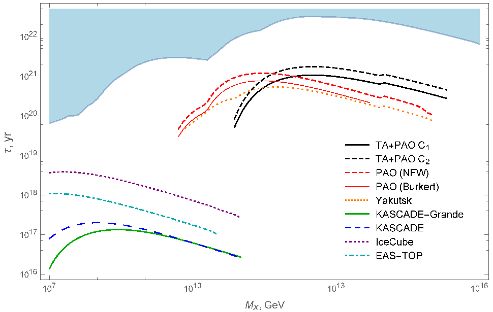
Another important feature is that the anisotropy constraints are stronger for the higher energies. This fact can be understood if we notice that the background isotropic cosmic–ray flux grows faster with the decrease of energy than the precision of anisotropy measurements. As it was anticipated the full–sky constraints surpass that of the limited sky coverage. The surprising fact is that second harmonic of full–sky analysis bounds $\tau$ stronger than the first one, although the theoretically predicted amplitude of the former is generally smaller (see below). This is the effect of the incidentally small value of the upper limit for one of the coefficients which is not compensated by the statistical penalty. The constrains by the third harmonic which are not shown in the figure are weaker than those by the first and second harmonic. The small bump around $M_{X}=10^{14}$ GeV on each curve is due to the accounting of galactic proton flux along with the photons, its impact on result is expectedly small.

For further experimental analysis development it is worth to discuss the maximal expected large–scale anisotropy from DM decay allowed by the most recent gamma–ray constraints [39]. We obtain it for the particular experiments and for the full–sky measurements by fixing the value of $\tau$ which is marginally allowed by the gamma–ray limits. The results for the range of masses $M_{X}$ are shown in Figs. 4–5 together with the recent limits. For the individual experiments we calculate the desired anisotropy sensitivity in terms of $r_{1}$. Variation of $r_{1}$ with the choice of an experiment reflects the fact that the anisotropy observed in particular experiment depends on its field of view. We use Pierre Auger and Telescope Array for medium and high energies and IceCube for lower energies. Increase in sensitivity and expanding of the energy range is expected in Telescope Array with the planned deployment of the low energy extension TALE [74], which will allow to collect events with the energies down to $10^{16}$ eV. The high area extension TA$\times$4 [75, 74] should give significant increase of the statistics at higher energies. One should note that the Southern hemisphere based experiments — Pierre Auger and IceCube have an advantage in galactic anisotropy study over the Northern hemisphere based Telescope Array because of more convenient position relative to the Galactic Center. We see that significant increase in experimental sensitivity to the large–scale anisotropy is need to detect the maximal signal expected from the DM decay. The IceCube sensitivity should be increased by roughly two orders of magnitude, while for Auger the respective values are from $\sim 10^{4}$ to $\sim 20$ times at 1 EeV energy.

For the full–sky analysis we present the predictions in therms of the first two angular power spectrum coefficients $C_{1}$ and $C_{2}$. While the full–sky constraints shown in Fig. 3 were imposed using the sets of coefficients $a_{1m}$ and $a_{2m}$, the power spectrum $C_{l}$ reveals the overall sensitivity of certain harmonic to the respective theoretical anisotropy pattern. In this sense the predictions shown are conservative. From the Figs. 4–5 one can learn that the large energies area is most opportune for the DM decay anisotropy search, while at the energies of $\sim 10$ EeV the sensitivity need to be increased by at least several hundred times comparing to the recent searches.

The obtained results indicate that current EAS experiments are more sensitive to the photons from DM decay than to the respective anisotropy. This occurs due to relatively the good hadron–photon primaries separation in EAS analysis and due to insufficient sensitivity of the ground based EAS experiments to the large scale anisotropy. A natural obstacle here is the necessity to combine the results of two experiments for the full–sky analysis. We should also note the connection between the anisotropy and gamma–ray signal. The large–scale anisotropy if observed at a particular energy not accompanied by the gamma–rays should be attributed to physics other than the DM decay, e.g. to the imprint of Large Scale Structure of the Universe [44, 45, 46, 47] or the anisotropic particle acceleration in the local cosmos [40, 41, 80]. In other words, until the gamma–rays of the respective energies are detected the DM signal should not interfere with the study of astrophysical large–scale anisotropy.

Some of the future experiments may be more sensitive to anisotropy than to gamma–ray DM signal. For instance the EUSO experiment is planned to have high sensitivity to anisotropy[81] while its ability of photon–hadron primaries separation is expected to be lower that in current experiments [82]. In Ref [79] the anisotropy detection prospects from the DM decay signal allowed by current photon limits were found favourable for EUSO experiment at ultra–high energies. At the same time planned photon sensitivity improvements in the currently running experiments - Pierre Auger and Telescope Array (see Ref.[83] for details) would make them even more effective in search for the signal of heavy decaying DM.

We would like to thank V. Rubakov, S. Troitsky and G. Rubtsov for helpful discussions. We are especially indebted to R. Aloisio, V. Berezinsky and M. Kachelriess for providing the numerical code solving the DGLAP equations. This work has been supported by the Russian Science Foundation grant 14-22-00161.

References

- [1] V. A. Kuzmin and V. A. Rubakov. Ultrahigh-energy cosmic rays: A Window to postinflationary reheating epoch of the universe? Phys. Atom. Nucl., 61:1028, 1998. arXiv:astro-ph/9709187.
- [2] V. Berezinsky, M. Kachelriess, and A. Vilenkin. Ultrahigh-energy cosmic rays without GZK cutoff. Phys. Rev. Lett., 79:4302–4305, 1997. arXiv:astro-ph/9708217, doi:10.1103/PhysRevLett.79.4302.
- [3] Ya. B. Zeldovich and Alexei A. Starobinsky. Particle production and vacuum polarization in an anisotropic gravitational field. Sov. Phys. JETP, 34:1159–1166, 1972. [Zh. Eksp. Teor. Fiz.61,2161(1971)].
- [4] Ya. B. Zeldovich and A. A. Starobinsky. Rate of particle production in gravitational fields. JETP Lett., 26:252–255, 1977. [Zh. Eksp. Teor. Fiz.26,373(1977)].
- [5] Lev Kofman, Andrei D. Linde, and Alexei A. Starobinsky. Reheating after inflation. Phys. Rev. Lett., 73:3195–3198, 1994. arXiv:hep-th/9405187, doi:10.1103/PhysRevLett.73.3195.
- [6] S. Yu. Khlebnikov and I. I. Tkachev. Resonant decay of Bose condensates. Phys. Rev. Lett., 79:1607–1610, 1997. arXiv:hep-ph/9610477, doi:10.1103/PhysRevLett.79.1607.
- [7] S. Yu. Khlebnikov and I. I. Tkachev. The Universe after inflation: The Wide resonance case. Phys. Lett., B390:80–86, 1997. arXiv:hep-ph/9608458, doi:10.1016/S0370-2693(96)01419-0.
- [8] Vadim Kuzmin and Igor Tkachev. Matter creation via vacuum fluctuations in the early universe and observed ultrahigh-energy cosmic ray events. Phys. Rev., D59:123006, 1999. arXiv:hep-ph/9809547, doi:10.1103/PhysRevD.59.123006.
- [9] Daniel J. H. Chung, Edward W. Kolb, and Antonio Riotto. Production of massive particles during reheating. Phys. Rev., D60:063504, 1999. arXiv:hep-ph/9809453, doi:10.1103/PhysRevD.60.063504.
- [10] Daniel J. H. Chung, Edward W. Kolb, and Antonio Riotto. Superheavy dark matter. Phys. Rev., D59:023501, 1999. arXiv:hep-ph/9802238, doi:10.1103/PhysRevD.59.023501.
- [11] Vadim Kuzmin and Igor Tkachev. Ultrahigh-energy cosmic rays, superheavy long living particles, and matter creation after inflation. JETP Lett., 68:271–275, 1998. [Pisma Zh. Eksp. Teor. Fiz.68,255(1998)]. arXiv:hep-ph/9802304, doi:10.1134/1.567858.
- [12] M. Yu. Khlopov and V. M. Chechetkin. Anti-protons in the Universe as Cosmological Test of Grand Unification. (In Russian). Fiz. Elem. Chast. Atom. Yadra, 18:627–677, 1987.
- [13] Daniele Fargion, M. Yu. Khlopov, R. V. Konoplich, V. R. Konoplich, and R. Mignani. On the possibility of detecting the annihilation of very heavy neutrinos in the galactic halo by 1-km**3 neutrino detector. Mod. Phys. Lett., A11:1363–1370, 1996. doi:10.1142/S0217732396001375.
- [14] Paolo Gondolo, Graciela Gelmini, and Subir Sarkar. Cosmic neutrinos from unstable relic particles. Nucl. Phys., B392:111–136, 1993. arXiv:hep-ph/9209236, doi:10.1016/0550-3213(93)90199-Y.
- [15] Masahiro Takeda et al. Energy determination in the Akeno Giant Air Shower Array experiment. Astropart. Phys., 19:447–462, 2003. arXiv:astro-ph/0209422, doi:10.1016/S0927-6505(02)00243-8.
- [16] T. Abu-Zayyad et al. The Cosmic Ray Energy Spectrum Observed with the Surface Detector of the Telescope Array Experiment. Astrophys. J., 768:L1, 2013. arXiv:1205.5067, doi:10.1088/2041-8205/768/1/L1.
- [17] J. Abraham et al. Observation of the suppression of the flux of cosmic rays above eV. Phys. Rev. Lett., 101:061101, 2008. arXiv:0806.4302, doi:10.1103/PhysRevLett.101.061101.
- [18] Kohta Murase, Ranjan Laha, Shin’ichiro Ando, and Markus Ahlers. Testing the Dark Matter Scenario for PeV Neutrinos Observed in IceCube. Phys. Rev. Lett., 115(7):071301, 2015. arXiv:1503.04663, doi:10.1103/PhysRevLett.115.071301.
- [19] Atri Bhattacharya, Mary Hall Reno, and Ina Sarcevic. Reconciling neutrino flux from heavy dark matter decay and recent events at IceCube. JHEP, 06:110, 2014. arXiv:1403.1862, doi:10.1007/JHEP06(2014)110.
- [20] Arman Esmaili and Pasquale Dario Serpico. Are IceCube neutrinos unveiling PeV-scale decaying dark matter? JCAP, 1311:054, 2013. arXiv:1308.1105, doi:10.1088/1475-7516/2013/11/054.
- [21] P. S. Bhupal Dev, D. Kazanas, R. N. Mohapatra, V. L. Teplitz, and Yongchao Zhang. Heavy right-handed neutrino dark matter and PeV neutrinos at IceCube. JCAP, 1608(08):034, 2016. arXiv:1606.04517, doi:10.1088/1475-7516/2016/08/034.
- [22] Arman Esmaili, Sin Kyu Kang, and Pasquale Dario Serpico. IceCube events and decaying dark matter: hints and constraints. JCAP, 1412(12):054, 2014. arXiv:1410.5979, doi:10.1088/1475-7516/2014/12/054.
- [23] Carsten Rott, Kazunori Kohri, and Seong Chan Park. Superheavy dark matter and IceCube neutrino signals: Bounds on decaying dark matter. Phys. Rev., D92(2):023529, 2015. arXiv:1408.4575, doi:10.1103/PhysRevD.92.023529.
- [24] M. G. Aartsen et al. Evidence for High-Energy Extraterrestrial Neutrinos at the IceCube Detector. Science, 342:1242856, 2013. arXiv:1311.5238, doi:10.1126/science.1242856.
- [25] M. G. Aartsen et al. Observation of High-Energy Astrophysical Neutrinos in Three Years of IceCube Data. Phys. Rev. Lett., 113:101101, 2014. arXiv:1405.5303, doi:10.1103/PhysRevLett.113.101101.
- [26] M. Yu. Kuznetsov. Hadronically decaying heavy dark matter and high-energy neutrino limits. 2016. arXiv:1611.08684.
- [27] Timothy Cohen, Kohta Murase, Nicholas L. Rodd, Benjamin R. Safdi, and Yotam Soreq. Gamma-ray Constraints on Decaying Dark Matter and Implications for IceCube. 2016. arXiv:1612.05638.
- [28] Brian Feldstein, Alexander Kusenko, Shigeki Matsumoto, and Tsutomu T. Yanagida. Neutrinos at IceCube from Heavy Decaying Dark Matter. Phys. Rev., D88(1):015004, 2013. arXiv:1303.7320, doi:10.1103/PhysRevD.88.015004.
- [29] Nagisa Hiroshima, Ryuichiro Kitano, Kazunori Kohri, and Kohta Murase. High-energy Neutrinos from Multi-body Decaying Dark Matter. 2017. arXiv:1705.04419.
- [30] Dmitry S. Gorbunov and Valery A. Rubakov. Introduction to the theory of the early universe: Hot big bang theory. World Scientific, Hackensack, 2011. URL: http://www.DESY.eblib.com/patron/FullRecord.aspx?p=737614.
- [31] Edward W. Kolb, Daniel J. H. Chung, and Antonio Riotto. WIMPzillas! In Trends in theoretical physics II. Proceedings, 2nd La Plata Meeting, Buenos Aires, Argentina, November 29-December 4, 1998, pages 91–105, 1998. [,91(1998)]. URL: http://lss.fnal.gov/cgi-bin/find_paper.pl?conf-98-325, arXiv:hep-ph/9810361.
- [32] Vadim A. Kuzmin and Igor I. Tkachev. Ultrahigh-energy cosmic rays and inflation relics. Phys. Rept., 320:199–221, 1999. arXiv:hep-ph/9903542, doi:10.1016/S0370-1573(99)00064-2.
- [33] Daniel J. H. Chung, Edward W. Kolb, Antonio Riotto, and Leonardo Senatore. Isocurvature constraints on gravitationally produced superheavy dark matter. Phys. Rev., D72:023511, 2005. arXiv:astro-ph/0411468, doi:10.1103/PhysRevD.72.023511.
- [34] D. S. Gorbunov and A. G. Panin. Free scalar dark matter candidates in -inflation: the light, the heavy and the superheavy. Phys. Lett., B718:15–20, 2012. arXiv:1201.3539, doi:10.1016/j.physletb.2012.10.015.
- [35] Oleg E. Kalashev, G. I. Rubtsov, and Sergey V. Troitsky. Sensitivity of cosmic-ray experiments to ultra-high-energy photons: reconstruction of the spectrum and limits on the superheavy dark matter. Phys. Rev., D80:103006, 2009. arXiv:0812.1020, doi:10.1103/PhysRevD.80.103006.
- [36] Kohta Murase and John F. Beacom. Constraining Very Heavy Dark Matter Using Diffuse Backgrounds of Neutrinos and Cascaded Gamma Rays. JCAP, 1210:043, 2012. arXiv:1206.2595, doi:10.1088/1475-7516/2012/10/043.
- [37] R. Aloisio, S. Matarrese, and A. V. Olinto. Super Heavy Dark Matter in light of BICEP2, Planck and Ultra High Energy Cosmic Rays Observations. JCAP, 1508(08):024, 2015. arXiv:1504.01319, doi:10.1088/1475-7516/2015/08/024.
- [38] Arman Esmaili and Pasquale Dario Serpico. Gamma-ray bounds from EAS detectors and heavy decaying dark matter constraints. JCAP, 1510(10):014, 2015. arXiv:1505.06486, doi:10.1088/1475-7516/2015/10/014.
- [39] O. K. Kalashev and M. Yu. Kuznetsov. Constraining heavy decaying dark matter with the high energy gamma-ray limits. Phys. Rev., D94(6):063535, 2016. arXiv:1606.07354, doi:10.1103/PhysRevD.94.063535.
- [40] Markus Ahlers. Deciphering the Dipole Anisotropy of Galactic Cosmic Rays. Phys. Rev. Lett., 117(15):151103, 2016. arXiv:1605.06446, doi:10.1103/PhysRevLett.117.151103.
- [41] Markus Ahlers. Anomalous Anisotropies of Cosmic Rays from Turbulent Magnetic Fields. Phys. Rev. Lett., 112(2):021101, 2014. arXiv:1310.5712, doi:10.1103/PhysRevLett.112.021101.
- [42] Philipp Mertsch and Stefan Funk. Solution to the cosmic ray anisotropy problem. Phys. Rev. Lett., 114(2):021101, 2015. arXiv:1408.3630, doi:10.1103/PhysRevLett.114.021101.
- [43] Gwenael Giacinti and Gunter Sigl. Local Magnetic Turbulence and TeV-PeV Cosmic Ray Anisotropies. Phys. Rev. Lett., 109:071101, 2012. arXiv:1111.2536, doi:10.1103/PhysRevLett.109.071101.
- [44] Guenter Sigl, Francesco Miniati, and Torsten A. Ensslin. Ultrahigh-energy cosmic rays in a structured and magnetized universe. Phys. Rev., D68:043002, 2003. arXiv:astro-ph/0302388, doi:10.1103/PhysRevD.68.043002.
- [45] Gunter Sigl, Francesco Miniati, and Torsten A. Ensslin. Ultrahigh energy cosmic ray probes of large scale structure and magnetic fields. Phys. Rev., D70:043007, 2004. arXiv:astro-ph/0401084, doi:10.1103/PhysRevD.70.043007.
- [46] Oleg E. Kalashev, B. A. Khrenov, P. Klimov, S. Sharakin, and Sergey V. Troitsky. Global anisotropy of arrival directions of ultrahigh-energy cosmic rays: capabilities of space-based detectors. JCAP, 0803:003, 2008. arXiv:0710.1382, doi:10.1088/1475-7516/2008/03/003.
- [47] Hylke B. J. Koers and Peter Tinyakov. Testing large-scale (an)isotropy of ultra-high energy cosmic rays. JCAP, 0904:003, 2009. arXiv:0812.0860, doi:10.1088/1475-7516/2009/04/003.
- [48] M. Aglietta et al. Evolution of the cosmic ray anisotropy above eV. Astrophys. J., 692:L130–L133, 2009. arXiv:0901.2740, doi:10.1088/0004-637X/692/2/L130.
- [49] M. G. Aartsen et al. Anisotropy in Cosmic-ray Arrival Directions in the Southern Hemisphere Based on six Years of Data From the Icecube Detector. Astrophys. J., 826(2):220, 2016. arXiv:1603.01227, doi:10.3847/0004-637X/826/2/220.
- [50] T. Antoni et al. Large scale cosmic - ray anisotropy with KASCADE. Astrophys. J., 604:687–692, 2004. arXiv:astro-ph/0312375, doi:10.1086/382039.
- [51] Andrea Chiavassa et al. A study of the first harmonic of the large scale anisotropies with the KASCADE-Grande experiment. PoS, ICRC2015:281, 2016.
- [52] Alexander Aab et al. Searches for Large-Scale Anisotropy in the Arrival Directions of Cosmic Rays Detected above Energy of eV at the Pierre Auger Observatory and the Telescope Array. Astrophys. J., 794(2):172, 2014. arXiv:1409.3128, doi:10.1088/0004-637X/794/2/172.
- [53] A. A. Ivanov, A. D. Krasilnikov, M. I. Pravdin, and A. V. Sabourov. Large-scale distribution of cosmic rays in right ascension as observed by the Yakutsk array at energies above eV. Astropart. Phys., 62:1–6, 2015. arXiv:1407.1583, doi:10.1016/j.astropartphys.2014.07.002.
- [54] Alexander Aab et al. Multi-resolution anisotropy studies of ultrahigh-energy cosmic rays detected at the Pierre Auger Observatory. Submitted to: JCAP, 2016. arXiv:1611.06812.
- [55] Imen Al Samarai. Indications of anisotropy at large angular scales in the arrival directions of cosmic rays detected at the Pierre Auger Observatory. PoS, ICRC2015:372, 2016.
- [56] R. Aloisio, V. Berezinsky, and M. Kachelriess. Fragmentation functions in SUSY QCD and UHECR spectra produced in top - down models. Phys. Rev., D69:094023, 2004. arXiv:hep-ph/0307279, doi:10.1103/PhysRevD.69.094023.
- [57] Subir Sarkar and Ramon Toldra. The High-energy cosmic ray spectrum from relic particle decay. Nucl. Phys., B621:495–520, 2002. arXiv:hep-ph/0108098, doi:10.1016/S0550-3213(01)00565-X.
- [58] V. N. Gribov and L. N. Lipatov. Deep inelastic e p scattering in perturbation theory. Sov. J. Nucl. Phys., 15:438–450, 1972. [Yad. Fiz.15,781(1972)].
- [59] L. N. Lipatov. The parton model and perturbation theory. Sov. J. Nucl. Phys., 20:94–102, 1975. [Yad. Fiz.20,181(1974)].
- [60] Yuri L. Dokshitzer. Calculation of the Structure Functions for Deep Inelastic Scattering and e+ e- Annihilation by Perturbation Theory in Quantum Chromodynamics. Sov. Phys. JETP, 46:641–653, 1977. [Zh. Eksp. Teor. Fiz.73,1216(1977)].
- [61] Guido Altarelli and G. Parisi. Asymptotic Freedom in Parton Language. Nucl. Phys., B126:298–318, 1977. doi:10.1016/0550-3213(77)90384-4.
- [62] M. Hirai, S. Kumano, T. H. Nagai, and K. Sudoh. Determination of fragmentation functions and their uncertainties. Phys. Rev., D75:094009, 2007. arXiv:hep-ph/0702250, doi:10.1103/PhysRevD.75.094009.
- [63] Dmitri Ivanov. TA Spectrum Summary. PoS, ICRC2015:349, 2016.
- [64] M. Amenomori et al. The All-particle spectrum of primary cosmic rays in the wide energy range from 10**14 eV to 10**17 eV observed with the Tibet-III air-shower array. Astrophys. J., 678:1165–1179, 2008. arXiv:0801.1803, doi:10.1086/529514.
- [65] K. A. Olive et al. Review of Particle Physics. Chin. Phys., C38:090001, 2014. doi:10.1088/1674-1137/38/9/090001.
- [66] Marco Cirelli, Gennaro Corcella, Andi Hektor, Gert Hutsi, Mario Kadastik, Paolo Panci, Martti Raidal, Filippo Sala, and Alessandro Strumia. PPPC 4 DM ID: A Poor Particle Physicist Cookbook for Dark Matter Indirect Detection. JCAP, 1103:051, 2011. [Erratum: JCAP1210,E01(2012)]. arXiv:1012.4515, doi:10.1088/1475-7516/2012/10/E01,10.1088/1475-7516/2011/03/051.
- [67] Julio F. Navarro, Carlos S. Frenk, and Simon D. M. White. The Structure of cold dark matter halos. Astrophys. J., 462:563–575, 1996. arXiv:astro-ph/9508025, doi:10.1086/177173.
- [68] Julio F. Navarro, Carlos S. Frenk, and Simon D. M. White. A Universal density profile from hierarchical clustering. Astrophys. J., 490:493–508, 1997. arXiv:astro-ph/9611107, doi:10.1086/304888.
- [69] A. Burkert. The Structure of dark matter halos in dwarf galaxies. IAU Symp., 171:175, 1996. [Astrophys. J.447,L25(1995)]. arXiv:astro-ph/9504041, doi:10.1086/309560.
- [70] O. E. Kalashev and E. Kido. Simulations of Ultra High Energy Cosmic Rays propagation. J. Exp. Theor. Phys., 120(5):790–797, 2015. arXiv:1406.0735, doi:10.1134/S1063776115040056.
- [71] Marijke Haverkorn. Magnetic Fields in the Milky Way. 2014. arXiv:1406.0283, doi:10.1007/978-3-662-44625-6_17.
- [72] P. Sommers. Cosmic ray anisotropy analysis with a full-sky observatory. Astropart. Phys., 14:271–286, 2001. arXiv:astro-ph/0004016, doi:10.1016/S0927-6505(00)00130-4.
- [73] M. Ackermann et al. Constraints on the Galactic Halo Dark Matter from Fermi-LAT Diffuse Measurements. Astrophys. J., 761:91, 2012. arXiv:1205.6474, doi:10.1088/0004-637X/761/2/91.
- [74] Hiroyuki Sagawa. Telescope Array extension. Nucl. Part. Phys. Proc., 279-281:145–152, 2016. doi:10.1016/j.nuclphysbps.2016.10.021.
- [75] Hiroyuki Sagawa. Telescope Array extension: TAx4. PoS, ICRC2015:657, 2016.
- [76] Julian Candia, Silvia Mollerach, and Esteban Roulet. Cosmic ray spectrum and anisotropies from the knee to the second knee. JCAP, 0305:003, 2003. arXiv:astro-ph/0302082, doi:10.1088/1475-7516/2003/05/003.
- [77] Antoine Calvez, Alexander Kusenko, and Shigehiro Nagataki. The role of Galactic sources and magnetic fields in forming the observed energy-dependent composition of ultrahigh-energy cosmic rays. Phys. Rev. Lett., 105:091101, 2010. arXiv:1004.2535, doi:10.1103/PhysRevLett.105.091101.
- [78] M. Kachelriess and Pasquale Dario Serpico. The Compton-Getting effect on ultra-high energy cosmic rays of cosmological origin. Phys. Lett., B640:225–229, 2006. arXiv:astro-ph/0605462, doi:10.1016/j.physletb.2006.08.006.
- [79] Luca Marzola and Federico R Urban. Ultra High Energy Cosmic Rays & Super-heavy Dark Matter. 2016. arXiv:1611.07180.
- [80] Yutaka Fujita, Kohta Murase, and Shigeo S. Kimura. Sagittarius A* as an Origin of the Galactic TeV-PeV Cosmic Rays? 2016. arXiv:1604.00003.
- [81] B. Rouillé d’Orfeuil, D. Allard, C. Lachaud, E. Parizot, C. Blaksley, and S. Nagataki. Anisotropy expectations for ultra-high-energy cosmic rays with future high statistics experiments. Astron. Astrophys., 567:A81, 2014. arXiv:1401.1119, doi:10.1051/0004-6361/201423462.
- [82] B. R. Dawson, M. Fukushima, and P. Sokolsky. Past, Present and Future of UHECR Observations. 2017. arXiv:1703.07897.
- [83] Timo Karg, Jaime Alvarez-Muñiz, Daniel Kuempel, Mariangela Settimo, Grigory Rubtsov, and Sergey Troitsky. Report from the Multi-Messenger Working Group at UHECR-2014 Conference. JPS Conf. Proc., 9:010021, 2016. arXiv:1510.02050, doi:10.7566/JPSCP.9.010021.