Big data analysis using shrinkage strategies

Let $n$ denote the sample size or number of observations and $p$ the number of features or variables. Data scientists consider big data as when $n$ is too large, however in medical and genetic researches, engineering and financial studies, one mostly involves small $n$ large $p$ problem, known as high-dimensional data. As Pyne et al., (2016) pointed in big data analytics, some domains of big data such as finance or health do even produce infinite dimensional functional data, which are observed not as points but functions, such as growth curves, online auction bidding trends, etc. As Wang et al., (2012) pointed, big data are data on a massive scale in terms of volume, intensity, and complexity that exceed the capacity of standard analytic tools. Ahmed, 2014b () collected some research contributions in the field of big data analytics to highlight high-dimensional methods in big data challenges.

As Ahmed and Yüzbaşı, 2016a () and Ahmed and Yüzbaşı, 2016b () pointed, the term “big data” is not well defined, but its problems are real and statisticians need to play a more important role in this arena. The big data or data science is an emerging field. In 2013, American Statistical Association (ASA) proposed three reasons to show ASA has not been very involved in big data. President of Institute of Mathematical Statistics (IMS), Bin Yu, in 2014 called for statisticians to own data science by working on real problems such as those from genomics, neuroscience, astronomy, nanoscience, computational social science, personalized medicine/healthcare, finance, and government; relevant methodology/theory will follow naturally.

There is an increasing demand for efficient prediction strategies for analyzing high-dimensional data in big data streams. For example, data arising from gene expression arrays, social network modeling, clinical, genetics and phenotypic data. Due to the trade-off between model complexity and model prediction, the statistical inference of model selection becomes an extremely important and challenging problem in high-dimensional data analysis. Over the past two decades, many penalized regularization approaches have been developed to do variable selection and estimation simultaneously. Among them, least absolute shrinkage and selection operator (LASSO) is one of the recent approaches, Tibshirani, (1996). It is a useful technique due to its convexity and computation efficiency. The LASSO is based on squared error and a penalty proportional to regression parameters. Schelldorfer et al., (2011) provides a comprehensive summary of the consistency properties of the LASSO. Efron et al., (2004) introduced the least angle regression algorithm which is a very fast way to draw the entire regularization path for a LASSO estimate of the regression parameters. The penalized likelihood methods have been extensively studied in the literature, see for example, Tran, (2011), Huang et al., (2008), Kim et al., (2008), Wang and Leng, (2012), Yuan and Lin, (2006), Leng et al., (2006), and Tibshirani et al., (2005). The penalized likelihood methods have a close connection to Bayesian procedures. Thus the LASSO estimate corresponds to a Bayes method that puts a Laplacian (double exponential) prior on the regression coefficients. Recent results (Armagan et al., (2013), Bhattacharya et al., (2012), and Carvalho et al., (2010)) have demonstrated that better desirable results can be obtained by using priors with heavier tails than the double exponential prior, in particular, priors with polynomial tails. Our study has concentrated on the widely recognized penalty estimators LASSO and adaptive LASSO (ALASSO). Very recently, Yüzbaşı and Arashi, (2016) have proposed double shrinking concept to improve the prediction accuracy of LASSO. Here, we specifically implement the double shrunken estimator on ALASSO.

Following Ahmed and Yüzbaşı, 2016a (), we consider the estimation problem of regression parameters when there are many potential predictors in the initial/working model and:

1. (1)

   most of them may not have any influence (sparse signals) on the response of interest

2. (2)

   some of the predictors may have strong influence (strong signals) on the response of interest

3. (3)

   some of them may have weak-moderate influence (weak-moderate signals) on the response of interest

It is possible that there may be extraneous predictors in the model. Suppose if the main concern is treatment effect, or the effect of biomarkers, extraneous nuisance variables may be lab effects when several labs are involved, or the age and sex of patients. The analysis will be more precise if “nuisance variables” can be left out of the model. This leads to the consideration of two models: the full model that includes all predictors and possible extraneous variables, and a candidate submodel that includes the predictors of main concern while leaving out extraneous variables. Further, it is important that we do not automatically remove all the predictors with weak signals from the model. This may result in selecting a biased submodel. A logical way to deal with this framework is to use pretest model selection and estimation strategies that test whether the coefficients of the extraneous variables are zero and then estimate parameters in the model that include coefficients that are rejected by the test. Another strategy is to use Stein-type shrinkage estimators where the estimated regression coefficient vector is shrunk in the direction of the candidate subspace. This “soft threshold” modification of the pretest method has been shown to be efficient in various frameworks. Ahmed et al., (2012), among others have investigated the properties of shrinkage and pretest methodologies for host models.

The model and some estimators are introduced in Section 2. In Section 3 we showcase our suggested estimation strategy. The results of a simulation study that includes comparison of suggested estimator with the penalty estimators are reported in Section 4. Application to real data sets is given in Section 5. Finally, we offer concluding remarks in Section 6.

In this communication, we consider a high-dimensional linear regression sparse model:

where $y_{i}$ observed response variable with predictors $x_{i}$s, and $\beta_{j}$ are the regression parameters. Further, $\varepsilon_{i}$s are independent and identically distributed random errors with center $0$ and variance $\sigma^{2}$. Similar to most of LASSO penalty-type models, in our approach, we assume the true model is sparse in the sense that most of regression coefficients are zeros except for a few ones and all nonzero $\beta_{j}$’s are larger than noise level, $c\sigma\sqrt{(2/n)\log(d)}$ with $c\geq 1/2$. We refer to Zhao and Yu, (2006), Huang et al., (2008), and Bickel et al., (2009) for some insights. In general, the LASSO penalty turns to select an over-fitted model since it penalizes all coefficients equally (Leng et al., (2006)). In reviewed literature several modification and methodologies have been suggested to improve the prediction accuracy for LASSO strategy. For example, the SCAD (Fan and Li, (2001)), adaptive LASSO, (Zou, (2006)), MCP (Zhang, (2010)) and Stein-type LASSO (Yüzbaşı and Arashi, (2016)) and several others. These methods select a submodel by shrinking some regression coefficients to zero and provide shrinkage estimators of the remaining coefficients. However, these methods may force the relatively more weak coefficients towards zeros as compared to LASSO, resulting in under-fitted models subject to a much larger selection bias in the presence of significant number of weak signals.

Following Ahmed and Yüzbaşı, 2016a () and Ahmed and Yüzbaşı, 2016b (), in this paper, we consider the estimation and prediction problem for the sparse regression models when there are many potential predictors that have weak influence on the response of interest. The analysis will be relatively more precise if “weak effect” variables can be weighted for the ultimate model prediction. This leads to the consideration of two models: the over-fitted model that includes predictors with strong signals and possibly some predictors with weak signals selected by LASSO. On the other, we select an underfitted model that possibly includes the predictors with strong signals while leaving out predictors with weak effect by using ALASSO. One way to deal with this framework is to use Stein-type shrinkage estimators where the estimated regression coefficient vector is shrunk in the direction of the under-fitted model. This “soft threshold” modification of the pretest method has been shown to be efficient in various frameworks. Saleh, (2006) and Ahmed et al., (2012), among others have examined the properties of Stein-type shrinkage estimation strategies for a host of models.

Consider the following regression model

where ${\mathbf{Y}}=(y_{1},y_{2},\dots,y_{n})^{\prime}$ is a vector of responses, ${\mathbf{X}}_{n}$ is an $n\times p$ fixed design matrix, $\bm{\beta}=(\beta_{1},\dots,\beta_{p})^{\prime}$ is an unknown vector of parameters, $\bm{\varepsilon}=(\varepsilon_{1},\varepsilon_{2},\dots,\varepsilon_{n})^{\prime}$ is the vector of unobservable random errors, and the superscript (^′) denotes the transpose of a vector or matrix. We do not make any distributional assumption about the errors except that $\bm{\varepsilon}$ has a cumulative distribution function $F(\bm{\varepsilon})$ with $E(\bm{\varepsilon})=\bm{0}$, and $E(\bm{\varepsilon}\bm{\varepsilon}^{\prime})=\sigma^{2}\bm{I}$, where $\sigma^{2}$ is finite.

For $n>p$ the classical estimator of $\bm{\beta}$ by minimizing the least square function and is given by

However, since we are dealing with a high-dimensional situation, i.e. $n<p$ so $({\mathbf{X}}^{\prime}{\mathbf{X}})^{-1}$ will not exist and thus no solution. However, one can employ the generalized inverse to revert the problem. In the current set-up we are assuming that the model is sparse so it is desirable to use penalized likelihood method to obtain a meaningful solution as was briefly discussed in our Introduction section. Penalty estimators are a class of estimators in the least penalized squares family of estimators, see Ahmed, 2014a (). This method involves penalizing the regression coefficients, and shrinking a subset of them to zero. In other words, the penalized procedure produces a submodel and subsequently estimates the submodel parameters. Several penalty estimators have been proposed in the literature for linear and generalized linear models. In this section, we consider the LASSO and the ALASSO. By shrinking some regression coefficients to zero, these methods select parameters and estimation simultaneously. Frank and Friedman, (1993) introduced bridge regression, a generalized version of penalty (or absolute penalty type) estimators. For a given penalty function $\pi(\cdot)$ and regularization parameter $\lambda$, the general form can be written as

where the penalty function is of the form

The penalty function in (2.3) bounds the $L_{\gamma}$ norm of the parameters in the given model as $\sum_{j=1}^{m}|\beta_{j}|^{\gamma}\leq t$, where $t$ is the tuning parameter that controls the amount of shrinkage. We see that for $\gamma=2$, we obtain ridge estimates which are obtained by minimizing the penalized residual sum of squares

where $\lambda$ is the tuning parameter which controls the amount of shrinkage. Frank and Friedman, (1993) did not solve for the bridge regression estimators for any $\gamma>0.$ Interestingly, for $\gamma<2$, it shrinks the coefficient towards zero, and depending on the value of $\lambda,$ it sets some of them to be exactly zero. Thus, the procedure combines variable selection and shrinking of the coefficients of penalized regression. Gao et al., (2016) suggested weighted ridge estimator for high dimensional setting, and investigated the advantages of post selection positive part of shrinkage estimators both theoretically and numerically.

An important member of the penalized least squares family is the $L_{1}$ penalized least squares estimator, which is obtained when $\gamma=1$, and is called LASSO.

In this section, we show how to shrink more the addressed penalized estimators, in the combination of two submodels produced by two distinct variable selection techniques. Similar to Ahmed and Yüzbaşı, 2016a (), the idea is to work with a sparse model that will be all the predictors included and then apply two variable selection methods with high and low penalties, respectively. Finally, we combine the estimates from two models to improve post estimation and prediction performances, respectively and incorporate the concept of double shrunken of Yüzbaşı and Arashi, (2016).

In this section, we develop some properties of the proposed estimators. Because of the complexity, we only consider orthonormal design. Note that in general, the LASSO is not an oracle procedure and is not consistent, whereas the ALASSO has oracle properties. Honestly, our result, is restrictive.

For our purpose, we assume $n^{-1}{\mathbf{X}}^{\prime}{\mathbf{X}}={\mathbf{I}}_{p}$. Under the specified partitioning, $n^{-1}{\mathbf{X}}_{S_{i}}^{\prime}{\mathbf{X}}_{S_{i}}={\mathbf{I}}_{p_{i}}$ and ${\mathbf{X}}_{S_{i}}^{\prime}{\mathbf{X}}_{S_{j}}=\bm{0}$, for $i\neq j=1,2,3$. Simply, $\bm{M}_{1}={\mathbf{I}}_{n}-{\mathbf{X}}_{S_{1}}{\mathbf{X}}_{S_{1}}^{\prime}$, ${\mathbf{X}}_{S_{2}}^{\prime}\bm{M}_{1}{\mathbf{X}}_{S_{2}}=n{\mathbf{I}}_{p_{2}}$, and

Further, we have

For the true parameter value, $|\hat{\beta}_{1j}|>\lambda/2$, for $j=1,\ldots,p_{o}<p_{1}$, where $p_{o}$ is the true parameter value for the active set $\{j:\beta_{j}\neq 0,j=1,\ldots,p_{1}\}$. Then, it is easy to see

Therefore, we can obtain the following bound

if $\lambda$ is suitably chosen such that $\lambda<2$.

Define the risk function of any estimator $\hat{\bm{\beta}}_{1}$ of true parameter ${\bm{\beta}}_{1}$ by ${\rm R}({\bm{\beta}}_{1};\hat{\bm{\beta}}_{1})=\mathbb{E}(\hat{\bm{\beta}}_{1}-{\bm{\beta}}_{1})^{\prime}(\hat{\bm{\beta}}_{1}-{\bm{\beta}}_{1})$. Note, here we have $j=1,\ldots,p_{o}$.

Then, under the orthonormal assumption, we have

As $n\to\infty$, $\bm{\widehat{\beta}}_{1}^{\rm OF}\overset{P}{\to}{\bm{\beta}}_{1}$. Hence, for sufficiently large samples size $n$, ${\rm R}({\bm{\beta}};\bm{\widehat{\beta}}_{1}^{\rm FS})<{\rm R}({\bm{\beta}};\bm{\widehat{\beta}}_{1}^{\rm OF})$, i.e., the proposed $\bm{\widehat{\beta}}_{1}^{\rm FS}$ outperforms $\bm{\widehat{\beta}}_{1}^{\rm OF}$ ($\bm{\widehat{\beta}}_{1}^{\rm FS}\succ\bm{\widehat{\beta}}_{1}^{\rm OF}$) as soon as $\sum_{j=1}^{p_{o}}{\rm sgn}(\hat{\beta}_{j}^{\rm LSE})<0$, under a probabilistic sense. This scenario is independent of the choice of $r(\cdot)$ and hence, all the shrinkage estimators outperform the over fitted model. Similar conclusion can be discovered for the under fitted model, with a slightly different condition.

In general, $\bm{\widehat{\beta}}_{1}^{\rm FS}\succ\bm{\widehat{\beta}}_{1}^{\rm OF}$ iff for all $r(\cdot)$, we have

Let

Then, $\alpha$ satisfies $\sqrt{n}(\bm{\widehat{\beta}}_{1}^{\rm OF}-{\bm{\beta}}_{1})=\alpha\sqrt{n}(\bm{\widehat{\beta}}_{1}^{\rm OF}-\bm{\widehat{\beta}}_{1}^{\rm UF})=\alpha\left[\sqrt{n}(\bm{\widehat{\beta}}_{1}^{\rm OF}-{\bm{\beta}}_{1})-\sqrt{n}(\bm{\widehat{\beta}}_{1}^{\rm UF}-{\bm{\beta}}_{1})\right]$. Let $\lambda=o(\sqrt{n})$ and $\lambda n^{(\gamma-1)/2}\to\infty$. Using Theorem 2 of Zou, (2006), $\sqrt{n}(\bm{\widehat{\beta}}_{1}^{\rm UF}-{\bm{\beta}}_{1})\overset{P}{\to}0$. Consequently $\alpha\to 1$. Now, we are ready to find the bound on $r(W_{n})/W_{n}$.

Suppose $r(\cdot)>0$ and is concave. Then, using Lemma 1 of Casella, (1990), $r(W_{n})/W_{n}$ is non-increasing. Hence, by (4.9), $\bm{\widehat{\beta}}_{1}^{\rm FS}\succ\bm{\widehat{\beta}}_{1}^{\rm OF}$ if for every $r$ function we have

We consider a Monte Carlo simulation, and simulate the response from the following model:

where $\varepsilon_{i}$ are i.i.d. $N\left(0,1\right)$ and ${x}_{ij}=(\xi_{(ij)}^{1})^{2}+\xi_{(ij)}^{2}$ with $\xi_{(ij)}^{1}\sim N\left(0,1\right)$ and $\xi_{(ij)}^{2}\sim N\left(0,1\right)$ for all $i=1,2,...,n$, $j=1,2,...,p$.

We consider the regression coefficients are set ${\bm{\beta}}=\left({\bm{\beta}}_{1}^{\prime},{\bm{\beta}}_{2}^{\prime},{\bm{\beta}}_{3}^{\prime}\right)^{\prime}=\left(\bm{\Lambda}^{\prime}_{p_{1}},\bm{\Delta}^{\prime}_{p_{2}},\bm{0}_{p_{3}}^{\prime}\right)^{\prime}$, where, $\bm{\Lambda}_{p_{1}}$, $\bm{\Delta}_{p_{2}}$ and $\bm{0}_{p_{3}}$ mean the vectors of $\Lambda$, $\Delta$ and 0 with dimensions $p_{1}$, $p_{2}$ and $p_{3}$, respectively. If $\Delta=0$, then it indicates that the null hypothesis is true. On the other hand, the larger values $\Delta$ indicate the degree of violation of null hypothesis.

In this simulation setting, we simulated 250 data sets consisting of $n=150$, $\Lambda=1,2$, $p_{1}=4$, $p_{2}=4,8,16$ and $p_{3}=200,400,800$.

The performance of an estimator is evaluated by using relative mean squared error (RMSE) criterion. The RMSE of an estimator $\bm{\beta}_{1}^{\ast}$ with respect to $\bm{\widehat{\beta}}_{1}^{\rm OF}$ is defined as follows

where $\bm{\beta}_{1}^{\ast}$ is one of the listed estimators. If the RMSE of an estimator is larger than one, it indicates that it is superior to $\bm{\widehat{\beta}}_{1}^{\rm OF}$. The results of simulated RMSE of the listed estimators are reported in Tables 2 – 7 and Figures 1 and 2. We also report the TP (the number of true positives) and the FP (the number of false positives) in Table 1 only for $(p_{2},p_{3})=(4,200)$.

According to the simulation results, the performance of under-fitted estimator ALASSO is the best since it is based on true model, and the FS3 performs better than both FS1 and PS when $\Delta=0$. On the other hand, the RMSE of the ALASSO decreases and approaches to zero while the all others approach to one when we increase the magnitude of weak signals.

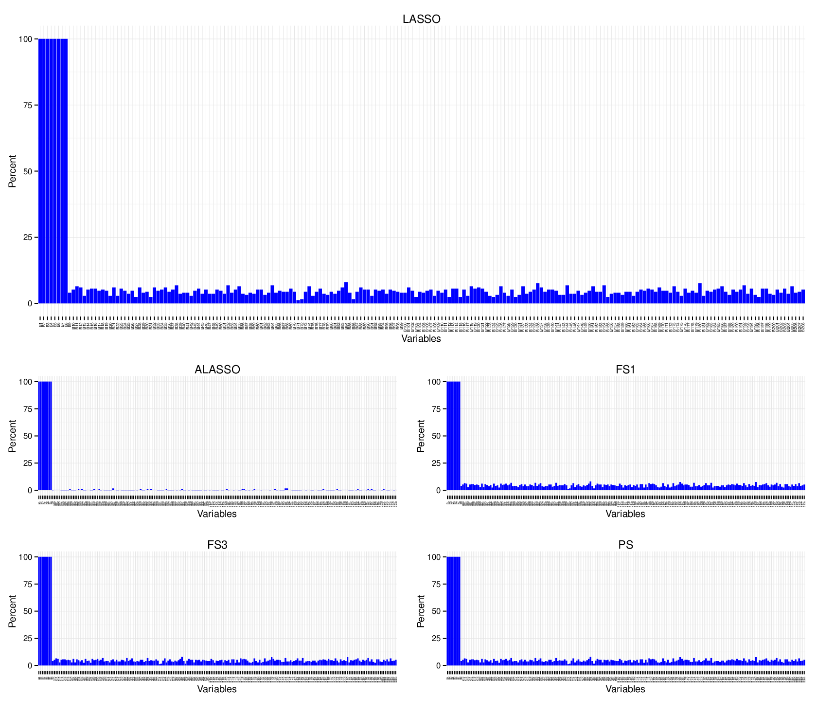
In Figure 1, if $\Delta=0$, then both LASSO and ALASSO methods always select strong covariates, while ALASSO select less weak signals than LASSO. Contrary to this, if we increase the magnitude of weak signals, say $\Delta=0.8$, then we observe that LASSO is more efficient than ALASSO for selecting those signals, see the Figure 2. For both case, our suggest methods again select all strong signals, while they select more variables than ALASSO when the weak signals are getting stronger.

Table 1 shows the numbers and the percentages of TP and FP of the listed estimators when $(p_{2},p_{3})=(4,200)$. According to this table, all listed methods select all strong covariates for each values of $\Delta$, whereas ALASSO is the best for FP, which is indicated by the smallest ratio of FP.

In this section, we analyze the performance of double shrinkage estimators dealing with two real data sets. We follow Ahmed and Yüzbaşı, 2016a () strategies for analyzing each data sets. As long as there is no uncertain prior information about $p_{1}$, $p_{2}$ and $p_{3}$, one may use LASSO and ALASSO methods to find important covariates. After that, we may construct our estimation strategies. We also indicate that we draw 1000 bootstrap sample with dimension of the design matrix, and we calculate the prediction error (PE) based on 5 - fold cross validation, and take its average value for each bootstrap sample. To easy comparison, we report relative PE (RPE) of an estimator with respect to LASSO. Thus, a value of RPE $>1$ reflects the superiority of the other methods.

In this paper, we extended variable selection methods to a new direction to be shrunken to a targeted estimator. Specifically we combined estimation strategies from both under-fitted and over-fitted models, in a high-dimensional regression model, employing a bounded measurable function. Specific concave functions were adopted to show the superiority of the proposed double shrunken estimators over the best of Ahmed and Yüzbaşı, 2016a (). We have conducted a simulation study to investigate the performance of the suggested shrinkage strategy with respect to two penalty estimators: LASSO and ALASSO. According to the simulation results, the performance of under-fitted estimator ALASSO is the best since it is based on true model, and the FS3 performs better than both FS1 and PS when $\Delta=0$. On the other hand, the RMSE of the ALASSO decreases and approaches to zero while the all others approach to one when we increase the magnitude of weak signals. We further analysed two high-dimensional data sets, and the performance of the shrinkage strategy was striking.

We also proposed another shrinkage estimator, which was not included in the numerical analyses, namely FS2 given by

We evaluated the performance of FS2 comparatively. We realized, it is not competitor to FS1, FS3 and PS, specially for small values $\Delta$. However, as soon as the non-centrality parameter $\Delta$ gets larger, its RMSE goes to 1 dominating all other estimators uniformly, since the weight goes to infinity and it simplifies to over-fitted model.

References

- (1) Ahmed, S.E. (2014a). Penalty, Shrinkage and Pretest Strategies: Variable Selection and Estimation, Springer, New York.
- (2) Ahmed, S.E. (2014b). Perspectives on Big Data Analysis: Methodologies and Applications, AMS, USA
- Ahmed et al., (2012) Ahmed, S. E., Hossain, S., & Doksum, K. A. (2012). LASSO and shrinkage estimation in Weibull censored regression models. Journal of Statistical Planning and Inference, 142(6), 1273-1284.
- (4) Ahmed, S. E., & Yüzbaşı, B. (2016a). Big data analytics: integrating penalty strategies, International Journal of Management Science and Engineering Management, 11(2), 105-115
- (5) Ahmed, S. E., & Yüzbaşı, B. (2016b). High Dimensional Data Analysis: Integrating Submodels. In Big and Complex Data Analysis (pp. 285-304). Springer International Publishing.
- Alam and Thompson, (1969) Alam, K., & Thompson, J. R. (1969). Locally averaged risk, Annals of Institute of Statistical Mathematics, 21, 457-469.
- Armagan et al., (2013) Armagan, A., Dunson, D. B., & Lee, J. (2013). Generalized double Pareto shrinkage. Statistica Sinica, 23(1), 119.
- Belloni and Chernozhukov, (2009) Belloni, A., & Chernozhukov, V. (2009). Least squares after model selection in high-dimensional sparse models.
- Bhattacharya et al., (2012) Bhattacharya, A., Pati, D., Pillai, N. S., & Dunson, D. B. (2012). Bayesian shrinkage. arXiv preprint arXiv:1212.6088.
- Bickel et al., (2009) Bickel, P.J., Ritov, Y. and Tsybakov, A.B. (2009). Simultaneous analysis of LASSO and dantzig selector, Annals of Statistics, 37, 1705–1732.
- Carvalho et al., (2010) Carvalho, C.M., Polson, N.G., & Scott, J.G. (2010). The horseshoe estimator for sparse signals, Biometrika 97, 465–480.
- Casella, (1990) Casella, G. (1990). Estimators with nondecreasing risk: Application of a chi-squared identity, Statistics & Probability Letter 10, 107–109.
- Efron et al., (2004) Efron, B., Hastie, T., Johnstone, I., & Tibshirani, R. (2004). Least angle regression. The Annals of statistics, 32(2), 407-499.
- Fan and Li, (2001) Fan, J., & Li, R. (2001). Variable selection via nonconcave penalized likelihood and its oracle properties. Journal of the American statistical Association, 96(456), 1348-1360.
- Frank and Friedman, (1993) Frank, I. and Friedman, J. (1993). A statistical view of some chemometrics regression tools (with discussion). Technometrics, 35, 109 – 148.
- Gao et al., (2016) Gao, X., Ahmed, S. E., & Feng, Y. (2016). Post Selection Shrinkage Estimation for High Dimensional Data Analysis. arXiv preprint arXiv:1603.07277.
- Hansen, (2015) Hansen, B. E. (2015). The risk of James–Stein and Lasso shrinkage. Econometric Reviews, 1-15.
- Huang et al., (2008) Huang, J., Ma, S., & Zhang, C. H. (2008). Adaptive LASSO for sparse high-dimensional regression models. Statistica Sinica, 1603-1618.
- Kim et al., (2008) Kim, Y., Choi, H., & Oh, H. S. (2008). Smoothly clipped absolute deviation on high dimensions. Journal of the American Statistical Association, 103(484), 1665-1673.
- Leng et al., (2006) Leng, C., Lin, Y., & Wahba, G. (2006). A note on the LASSO and related procedures in model selection. Statistica Sinica, 1273-1284.
- Liu and Yu, (2013) Liu, H., & Yu, B. (2013). Asymptotic properties of lasso+ mls and lasso+ ridge in sparse high-dimensional linear regression. Electronic Journal of Statistics, 7, 3124-3169.
- Pyne et al., (2016) Pyne, S., Rao, B.L.S. Prakasa and Rao, S.B.(2016). Big data analytics: Views from statistical and computational perspectives, in Big Data Analytics: Methods and Applications, 2016, Springer, India
- Saleh, (2006) Saleh, A. K. Md. Ehsanes. (2006). Theory of Preliminary Test and Stein-type Estimation with Applications, John Wiley, New York.
- Schelldorfer et al., (2011) Schelldorfer, J., Bühlmann, P., DE, G., & VAN, S. (2011). Estimation for High Dimensional Linear Mixed Effects Models Using - Penalization. Scandinavian Journal of Statistics, 38(2), 197-214.
- Scheetz et al., (2006) Scheetz, T. E., Kim, K. Y. A., Swiderski, R. E., Philp, A. R., Braun, T. A., Knudtson, K. L., … & Sheffield, V. C. (2006). Regulation of gene expression in the mammalian eye and its relevance to eye disease. Proceedings of the National Academy of Sciences, 103(39), 14429-14434.
- Tibshirani, (1996) Tibshirani, R. (1996). Regression shrinkage and selection via the LASSO. Journal of the Royal Statistical Society. Series B (Methodological), 267-288.
- Tibshirani et al., (2005) Tibshirani, R., Saunders, M., Rosset, S., Zhu, J., & Knight, K. (2005). Sparsity and smoothness via the fused LASSO. Journal of the Royal Statistical Society: Series B (Statistical Methodology), 67(1), 91-108.
- Tran, (2011) Tran, M. N. (2011). The loss rank criterion for variable selection in linear regression analysis. Scandinavian Journal of Statistics, 38(3), 466-479.
- Wang et al., (2012) Wang, C., Chen, M.H., Schifano, E., Wu, J. and Yan, J. (2015). Statistical methods and computing for big data, arXiv:1502.07989.
- Wang and Leng, (2012) Wang, H., & Leng, C. (2012). Unified LASSO estimation by least squares approximation. Journal of the American Statistical Association.
- Yuan and Lin, (2006) Yuan, M., & Lin, Y. (2006). Model selection and estimation in regression with grouped variables. Journal of the Royal Statistical Society: Series B (Statistical Methodology), 68(1), 49-67.
- Yüzbaşı and Arashi, (2016) Yuzbasi, B., & Arashi, M. (2016). Double shrunken selection operator, arXiv:1612.06304.
- Zhang, (2010) Zhang, C.H. (2010). Nearly unbiased variable selection under minimax concave penalty. Annals os Statistics, 38, 894 – 942.
- Zhang and Zhang, (2014) Zhang, C.H. and Zhang, S.S. (2014). Confidence intervals for low-dimensional parameters in high-dimensional linear models. Annals os Statistics, 76, 217–242.
- Zhao and Yu, (2006) Zhao, P., & Yu, B. (2006). On model selection consistency of LASSO. The Journal of Machine Learning Research, 7, 2541-2563.
- Zou, (2006) Zou, H. (2006). The adaptive LASSO and its oracle properties. Journal of the American statistical association, 101(476), 1418-1429.