The Power of Waiting for More than One Response in Minimizing the Age-of-Information
Abstract
The Age-of-Information (AoI) has recently been proposed as an important metric for investigating the timeliness performance in information-update systems. Prior studies on AoI optimization often consider a Push model, which is concerned about when and how to “push” (i.e., generate and transmit) the updated information to the user. In stark contrast, in this paper we introduce a new Pull model, which is more relevant for certain applications (such as the real-time stock quotes service), where a user sends requests to the servers to proactively “pull” the information of interest. Moreover, we propose to employ request replication to reduce the AoI. Interestingly, we find that under this new Pull model, replication schemes capture a novel tradeoff between different levels of information freshness and different response times across the servers, which can be exploited to minimize the expected AoI at the user’s side. Specifically, assuming Poisson updating process at the servers and exponentially distributed response time, we derive a closed-form formula for computing the expected AoI and obtain the optimal number of responses to wait for to minimize the expected AoI. Finally, we conduct numerical simulations to elucidate our theoretical results. Our findings show that waiting for more than one response can significantly reduce the AoI in most scenarios.
I Introduction
The last decades have witnessed the prevalence of smart devices and significant advances in ubiquitous computing and the Internet of things. This trend is forecasted to continue in the years to come [1]. The development of this trend has spawned a plethora of real-time services that require timely information/status updates. One practically important example of such services is vehicular networks and intelligent transportation systems [2, 3], where accurate status information (position, speed, acceleration, tire pressure, etc.) of a vehicle needs to be shared with other nearby vehicles and road-side facilities in a timely manner in order to avoid collisions and ensure substantially improved road safety. More such examples include sensor networks for environment/health monitoring [4, 5], wireless channel feedback [6], news feeds, weather updates, online social networks, fare aggregating sites (e.g., Google Shopping), and stock quotes service.
For systems providing such real-time services, those commonly used performance metrics, such as throughput and delay, exhibit significant limitations in measuring the system performance [7]. Instead, the timeliness of information updates becomes a major concern. To that end, a new metric called the Age-of-Information (AoI) has been proposed as an important metric for studying the timeliness performance [2]. The AoI is defined as the time elapsed since the most recent update occurred (see Eq. (1) for a formal definition). Using the AoI metric introduced in [2] for vehicular networks, the work of [7] employs a simple system model to analyze and optimize the timeliness performance of an information-update system. This seminal work has recently aroused dramatic interests from the research community and has inspired a series of interesting studies on the AoI analysis and optimization (see [8] and references therein).
While all prior studies consider a Push model, which is concerned about when and how to “push” (i.e., generate and transmit) the updated information to the user, in this paper we introduce a new Pull model, under which a user sends requests to the servers to proactively “pull” the information of interest. This Pull model is more relevant for many important applications where the user’s interest is in the freshness of information at the point when the user requests it rather than in continuously monitoring the freshness of information. One application of the Pull model is in the real-time stock quotes service, where a customer (i.e., user) submits a query to multiple stock quotes providers (i.e., servers) and each provider responds with the most up-to-date information it has.
To the best of our knowledge, however, none of the existing work on the timeliness optimization has considered such a Pull model. In stark contrast, we focus on the Pull model and propose to employ request replication to minimize the expected AoI at the user’s side. Although a similar Pull model is considered for data synchronization in [9, 10], the problems are quite different and request replication is not exploited. Note that the concept of replication is not new and has been extensively studied for various applications (e.g., cloud computing and datacenters [11, 12], storage clouds [13], parallel computing [14, 15], and databases [16, 17]). However, for the AoI minimization problem under the Pull model, replication schemes exhibit a unique property and capture a novel tradeoff between different levels of information freshness and different response times across the servers. This tradeoff reveals the power of waiting for more than one response and can be exploited to minimize the expected AoI at the user’s side.
Next, we explain the above key tradeoff through a comparison with cloud computing systems. It has been observed that in a cloud or a datacenter, the processing time of a same job can be highly variable on different servers [12]. Due to this important fact, replicating a job on multiple servers and waiting for the first finished copy can help reduce latency [12, 11]. Apparently, in such a system it is not beneficial to wait for more copies of the job to finish, as all the copies would give the same outcome. In contrast, in the information-update system we consider, although the servers may possess the same type of information (weather forecast, stock prices, etc.), they could have different versions of the information with different levels of freshness due to the random updating processes. Hence, the first response may come from a server with stale information; waiting for more than one response has the potential of receiving fresher information and thus helps reduce the AoI. Hence, it is no longer the best to stop after receiving the first response (as in the other aforementioned applications). On the other hand, waiting for too many responses will lead to a longer total waiting time and thus, also incurs a larger AoI at the user’s side. Therefore, it is challenging to determine the optimal number of responses to wait for in order to minimize the expected AoI at the user’s side.
In what follows, we summarize the key contributions of this paper. First, for the first time we introduce the Pull model for studying the timeliness optimization problem and propose to employ request replication to reduce the AoI. Second, assuming Poisson updating process at the servers and exponentially distributed response time, we derive a closed-form formula for computing the expected AoI and obtain the optimal number of responses to wait for to minimize the expected AoI. Some extensions are also discussed. Third, we conduct extensive numerical simulations to elucidate our theoretical results. We also investigate the impact of the system parameters (the updating rate, the mean response time, and the total number of servers) on the achieved gain in the AoI reduction. Simulation results for other types of response time distribution are also provided. Our findings show that waiting for more than one response can significantly reduce the AoI in most scenarios.
The remainder of this paper is organized as follows. We first describe our new Pull model in Section II. Then, we analyze the expected AoI under replication schemes in Section III, obtain the optimal number of responses for minimizing the expected AoI in Section IV, and briefly discuss some extensions of our work in Section V. Section VI presents the simulation results. Finally, we conclude the paper in Section VII.
II System Model
We consider an information-update system where a user pulls time-sensitive information from servers. These servers are connected to a common information source and update their data asynchronously. We call such a model the Pull model (see Fig. 1). Let be the server index. We assume that the information updating process at server is Poisson with rate and is independent and identically distributed (i.i.d.) across the servers. This implies that the inter-update time (i.e., the time duration between two successive updates) at each server follows an exponential distribution with mean . Here, the inter-update time at a server can be interpreted as the time required for the server to receive information updates from the source. Let denote the time when the most recent update at server occurs, and let denote the AoI at server , which is defined as the time elapsed since the most recent update at this server:
| (1) |
Therefore, if an update occurs at a server, then the AoI at this server drops to zero; otherwise, the AoI increases linearly as time goes by until the next update occurs. Fig. 2 provides an illustration of the AoI evolution at server .
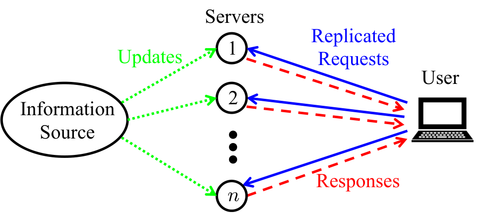

In this work, we consider the replication scheme, under which the user sends the replicated copies of the request to all servers and waits for the first responses. Let denote the response time for server . Note that each server may have a different response time, which is the time elapsed since the request is sent out by the user until the user receives the response from this server. We assume that the time for the requests to reach the servers is negligible compared to the time for the user to download the data from the servers. Hence, the response time can be interpreted as the downloading time. Let denote the downloading start time, which is the same for all the servers, and let denote the downloading finish time for server . Then, the response time for server is . We assume that the response time is exponentially distributed with mean and is i.i.d. across the servers. Note that the model we consider above is simple, but it suffices to capture the key aspects and novelty of the problem we study.
Under the replication scheme, when the user receives the first responses, it uses the freshest information among these responses to make certain decisions (e.g., stock trading decisions based on the received stock price information). Let denote the index of the server corresponding to the -th response received by the user. Then, set contains the indices of the servers that return the first responses, and the following is satisfied: and . Let server be the one that contains the freshest information (i.e., that has the smallest AoI) among these responses when downloading starts at time , i.e., (or due to Eq. (1)). Here, we are interested in the AoI at the user’s side when it receives the -th response, denoted by , which is the time difference between when the -th response is received and when the information at server is updated, i.e.,
| (2) |
Then, there are two natural questions of interest. First, for a given , can one obtain a closed-form formula for computing the expected AoI at the user’s side, ? Second, how to determine the optimal number of responses to wait for, such that is minimized? The second question can be formulated as the following optimization problem:
| (3) |
We will answer these two questions in the following two sections, respectively.
III Expected AoI
In this section, we focus on answering the first question and derive a closed-form formula for computing the expected AoI at the user’s side under the replication scheme.
We begin with the definition of and rewrite Eq. (2) as follows:
| (4) |
where (a) is from the definition of and and (b) is from the definition of (i.e., Eq. (1)). As can be seen from the above expression, under the replication scheme the AoI at the user’s side consists of two terms: (i) , the total waiting time for receiving the first responses, and (ii) (or ), the AoI of the freshest information among these responses when downloading starts at time . An illustration of these two terms and is shown in Fig. 3.
Taking the expectation of both sides of Eq. (4), we have
| (5) |
Intuitively, as increases, i.e., waiting for more responses, the expected total waiting time (i.e., the first term) increases. On the other hand, upon receiving more responses, the expected AoI of the freshest information among these responses (i.e., the second term) decreases. Hence, there is a natural tradeoff between these two terms, which is a unique property of our newly introduced Pull model.
Next, we formalize this tradeoff by deriving the closed-form expressions of the above two terms as well as the expected AoI. We state the main result of this section in Theorem 1.

Theorem 1.
Under the replication scheme, the expected AoI at the user’s side can be expressed as:
| (6) |
where is the -th partial sum of the diverging harmonic series.
Proof.
We first analyze the the first term of the right-hand side of Eq. (5) and want to show . Note that the response time is exponentially distributed with mean and is i.i.d. across the servers. Hence, random variable is the -th smallest value of i.i.d. exponential random variables with mean . The order statistics results of exponential random variables give that is an exponential random variable with mean and that is an exponential random variable with mean for any [18]. Hence, we have the following:
| (7) |
Next, we analyze the second term of the right-hand side of Eq. (5) and want to show the following:
| (8) |
Note that the updating process at each server is a Poisson process with rate and is i.i.d. across the servers. Hence, the inter-update time for each server is exponentially distributed with mean . Due to the memoryless property of the exponential distribution, the AoI at each server has the same distribution as the inter-update time, i.e., random variable is also exponentially distributed with mean and is i.i.d. across the servers [19]. Therefore, random variable is the minimum of i.i.d. exponential random variables with mean , which is also exponentially distributed with mean . This implies Eq. (8).
Remark. The above analysis indeed agrees with our intuition: while the expected total waiting time for receiving the first responses (i.e., Eq. (7)) is a monotonically increasing function of , the expected AoI of the freshest information among these responses (i.e., Eq. (8)) is a monotonically decreasing function of .
IV Optimal Replication Scheme
In this section, we will exploit the aforementioned tradeoff and focus on answering the second question we discussed at the end of Section II. Specifically, we aim to find the optimal number of responses to wait for in order to minimize the expected AoI at the user’s side.
Using the analytical result of Theorem 1, we rewrite the optimization problem in Eq. (3) as:
| (9) |
Let be an optimal solution to Eq. (9). We state the main result of this section in Theorem 2.
Theorem 2.
An optimal solution can be computed as:
| (10) |
Proof.
We first define as the difference of the expected AoI between the and replication schemes, i.e., for any . From Eq. (6), we have that for any ,
| (11) |
It is easy to see that is a monotonically increasing function of .
We now extend the domain of to the set of positive real numbers and want to find such that . With some standard calculations and dropping the negative solution, we derive the following:
| (12) |
Next, we discuss two cases: (i) and (ii) .
In Case (i), we have . This implies that for all due to the fact that is monotonically increasing. Hence, the expected AoI is a monotonically decreasing function for . Therefore, must be an optimal solution.
In Case (ii), we have . We consider two subcases: is an integer in and is not an integer.
If is an integer in , we have for and for . Hence, the expected AoI is first decreasing (for ) and then increasing (for ). Therefore, there are two optimal solutions: and since (due to ).
If is not an integer, we have for and for . Hence, the expected AoI is first decreasing (for ) and then increasing (for ). Therefore, must be an optimal solution.
Combining two subcases, we have in Case (ii). Then, combining Cases (i) and (ii), we have . ∎
Remark. There are two special cases that are of particular interest: waiting for the first response only (i.e., ) and waiting for all the responses (i.e., ). In Corollary 1, we provide a sufficient and necessary condition for each of these two special cases.
Corollary 1.
(i) is an optimal solution if and only if ; (ii) is an optimal solution if and only if .
Proof.
The proof follows straightforwardly from Theorem 2. A little thought gives the following: is an optimal solution if and only if . Solving gives . Similarly, is an optimal solution if and only if . Solving gives . ∎
Remark. The above results agree well with the intuition. For a given number of servers, if the mean inter-update time is much smaller than the mean response time (i.e., ), then all the servers have frequent updates and thus, the difference of the freshness levels among the servers is small. In this case, it is not beneficial to wait for more responses. On the other hand, if the mean inter-update time is much larger than the mean response time (i.e., ), then one server may possess fresher information than another server. In this case, it is worth waiting for more responses, which leads to a significant gain in the AoI reduction.
V Extensions
In this section, we discuss some extensions of our work.
Replication scheme. So far, we have only considered the replication scheme. One limitation of this scheme is that it requires the user to send a replicated request to every server, which may incur a large overhead when there are a large number of servers (i.e., when is large). Instead, a more practical scheme would be to send the replicated requests to a subset of servers. Hence, we consider the replication schemes, under which the user sends a replicated request to each of the servers that are randomly and uniformly chosen from the servers, and waits for the first responses, where and . Making the same assumptions as in Section II, we can derive the expected AoI at the user’s side in a similar manner. Specifically, reusing the proof of Theorem 1 and replacing with in the proof, we can show the following:
| (13) |
Uniformly distributed response time. Note that our current analysis requires the memoryless property of the Poisson updating process. However, the analysis can be extended to the uniformly distributed response time. We make the same assumptions as in Section II, except that the response time is now uniformly distributed in the range of with and . In this case, we have [18]. Since Eq. (8) still holds, from Eq. (5) we have
| (14) |
Following a similar line of analysis to that in the proof of Theorem 2, we can show that an optimal solution can be computed as:
| (15) |
VI Numerical Results
In this section, we perform extensive simulations to evaluate the AoI performance in an information-update system with servers under the replication scheme. We first describe our simulation settings. Throughout the simulations, the updating process at each server is assumed to be Poisson with rate and is i.i.d. across the servers. The user’s request for the information is generated at time , which is uniformly selected from the time interval , where we set . This implies that each server has a total of updates on average.
Next, we evaluate the AoI performance through simulations for three types of response time distribution: exponential, uniform, and Gamma. First, we assume that the response time is exponentially distributed with mean . Fig. 4(a) presents how the average AoI changes as the number of responses varies in three representative setups, where each point represents an average of simulation runs. We also include plots of our theoretical results (i.e., Eq. (6)) for comparison. A crucial observation from Fig. 4(a) is that the simulation results match perfectly with our theoretical results. In addition, we observe three different behaviors of the average AoI performance: (i) If the inter-update time is much smaller than the response time (i.e., , ), then the average AoI increases as increases and thus, it is not beneficial to wait for more than one response. (ii) In contrast, if the inter-update time is much larger than the response time (i.e., , ), then the average AoI decreases as increases and thus, it is worth waiting for all the responses so as to achieve a smaller average AoI. (iii) When the inter-update time is comparable to the response time (i.e., , ), then as increases, the AoI would first decrease and then increase. On the one hand, when is small, the freshness of the data at the servers dominates and thus, waiting for more responses helps reduce the average AoI. On the other hand, when becomes large, the total waiting time becomes dominant and thus, the average AoI increases as further increases.
In Section V, we discussed the extension of our theoretical results to the case of uniformly distributed response time. Hence, we also perform simulations for the response time uniformly distributed in the range of with mean . Fig. 4(b) presents the average AoI as the number of responses changes. In this scenario, the simulation results also match perfectly with the theoretical results (i.e., Eq. (14)). Also, we observe a very similar phenomenon to that in Fig. 4(a) on how the average AoI varies as increases in three different simulation setups.
In addition, Fig. 4(c) presents the simulation results for the response time with Gamma distribution, which can be used to model the response time in relay networks[20]. Specifically, we consider a special class of the Gamma() distribution that is the sum of i.i.d. exponential random variables with mean (which is also called the Erlang distribution). Then, the mean response time is equal to . We fix in the simulations. Although we are unable to derive analytical results in this case, the observations are similar to that under the exponential and uniform distributions.
Finally, we investigate the impact of the system parameters (the updating rate, the mean response time, and the total number of servers) on the optimal number of responses and the improvement ratio, defined as . The improvement ratio captures the gain in the AoI reduction under the optimal scheme compared to a naive scheme of waiting for the first response only.
Fig. 5(a) shows the impact of the updating rate . We observe that the optimal number of responses decreases as increases. This is because when the updating rate is large, the AoI diversity at the servers is small. In this case, waiting for more responses is unlikely to receive a response with much fresher information. Therefore, the optimal scheme will simply be a naive scheme that waits only for the first response when the updating rate is relatively large (e.g., ). Fig. 5(b) shows the impact of the mean response time . We observe that the optimal number of responses increases as increases. This is because when is large (i.e., when the mean response time is small), the cost of waiting for additional responses becomes marginal and thus, waiting for more responses is likely to lead to the reception of a response with fresher information. Fig. 5(c) shows the impact of the total number of servers . We observe that both the optimal number of responses and the improvement ratio increase with . This is because an increased number of servers leads to more diversity gains both in the AoI at the servers and in the response time.
VII Conclusion
In this paper, we introduced a new Pull model for studying the AoI minimization problem under the replication schemes. Assuming Poisson updating process and exponentially distributed response time, we derived the closed-form expression of the expected AoI at the user’s side and provided a formula for computing the optimal solution. Not only did our work reveal a novel tradeoff between different levels of information freshness and different response times across the servers, but we also demonstrated the power of waiting for more than one response in minimizing the expected AoI at the user’s side. An interesting direction for future work would be to develop dynamic replication schemes that do not require the knowledge of the updating process and the response time distribution.
References
- [1] “Cisco visual networking index: Global mobile data traffic forecast update, 2015–-2020,” February 2016, http://www.cisco.com/c/en/us/solutions/collateral/service-provider/visual-networking-index-vni/mobile-white-paper-c11-520862.pdf.
- [2] S. Kaul, M. Gruteser, V. Rai, and J. Kenney, “Minimizing age of information in vehicular networks,” in Proceedings of IEEE SECON, 2011, pp. 350–358.
- [3] S. Kaul, R. Yates, and M. Gruteser, “On piggybacking in vehicular networks,” in Proceedings of IEEE GLOBECOM, 2011, pp. 1–5.
- [4] J. Ko, C. Lu, M. B. Srivastava, J. A. Stankovic, A. Terzis, and M. Welsh, “Wireless sensor networks for healthcare,” Proceedings of the IEEE, vol. 98, no. 11, pp. 1947–1960, 2010.
- [5] P. Corke, T. Wark, R. Jurdak, W. Hu, P. Valencia, and D. Moore, “Environmental wireless sensor networks,” Proceedings of the IEEE, vol. 98, no. 11, pp. 1903–1917, 2010.
- [6] M. Costa, S. Valentin, and A. Ephremides, “On the age of channel state information for non-reciprocal wireless links,” in Proceedings of IEEE ISIT, 2015, pp. 2356–2360.
- [7] S. Kaul, R. Yates, and M. Gruteser, “Real-time status: How often should one update?” in Proceedings of IEEE INFOCOM, 2012, pp. 2731–2735.
- [8] Y. Sun, E. Uysal-Biyikoglu, R. D. Yates, C. E. Koksal, and N. B. Shroff, “Update or wait: How to keep your data fresh,” IEEE Transactions on Information Theory, in press, 2017.
- [9] L. Bright, A. Gal, and L. Raschid, “Adaptive pull-based data freshness policies for diverse update patterns,” University of Maryland, Tech. Rep., 2004. [Online]. Available: http://drum.lib.umd.edu/handle/1903/1334
- [10] ——, “Adaptive pull-based policies for wide area data delivery,” ACM Transactions on Database Systems, vol. 31, no. 2, pp. 631–671, 2006.
- [11] K. Gardner, S. Zbarsky, S. Doroudi, M. Harchol-Balter, and E. Hyytia, “Reducing latency via redundant requests: Exact analysis,” ACM SIGMETRICS Performance Evaluation Review, 2015.
- [12] G. Ananthanarayanan, A. Ghodsi, S. Shenker, and I. Stoica, “Why let resources idle? Aggressive cloning of jobs with dolly,” in The 4th USENIX Workshop on Hot Topics in Cloud Computing (HotCloud), 2012.
- [13] B. Li, A. Ramamoorthy, and R. Srikant, “Mean-field-analysis of coding versus replication in cloud storage systems,” in Proceedings of IEEE INFOCOM, 2016, pp. 1–9.
- [14] D. Wang, G. Joshi, and G. Wornell, “Efficient task replication for fast response times in parallel computation,” in ACM SIGMETRICS Performance Evaluation Review, vol. 42, no. 1, 2014, pp. 599–600.
- [15] ——, “Using straggler replication to reduce latency in large-scale parallel computing,” ACM SIGMETRICS Performance Evaluation Review, vol. 43, no. 3, pp. 7–11, 2015.
- [16] E. Pacitti, “Improving data freshness in replicated databases,” Ph.D. dissertation, INRIA, 1999.
- [17] J. Pereira and M. Araújo, “Evaluating data freshness in large scale replicated databases,” INForum 2010-II Simpósio de Informática, pp. 231–242, 2010.
- [18] B. C. Arnold, N. Balakrishnan, and H. N. Nagaraja, A first course in order statistics. SIAM, 2008.
- [19] R. Nelson, Probability, stochastic processes, and queueing theory: the mathematics of computer performance modeling. Springer Science & Business Media, 2013.
- [20] E. Najm and R. Nasser, “Age of information: The gamma awakening,” in Proceedings of IEEE ISIT, 2016.