Classicalization of Quantum State of Detector by Amplification Process

Arash Tirandaz Affiliation: Foundations of Physics Group, School of Physics, Institute for Research in Fundamental Sciences (IPM), P.O.Box 19395-5531, Tehran, Iran Farhad Taher Ghahramani Corresponding Author: farhadtqm@ipm.ir Affiliation: Foundations of Physics Group, School of Physics, Institute for Research in Fundamental Sciences (IPM), P.O.Box 19395-5531, Tehran, Iran Ali Asadian Affiliation: Department of Physics, Institute for Advanced Studies in Basic Sciences (IASBS), Gava Zang, Zanjan 45137-66731, Iran Affiliation: Naturwissenschaftlich-Technische Fakultät, Universität Siegen, Walter-Flex-Str. 3, D-57068 Siegen, Germany Mehdi Golshani Affiliation: Foundations of Physics Group, School of Physics, Institute for Research in Fundamental Sciences (IPM), P.O.Box 19395-5531, Tehran, Iran Affiliation: Department of Physics, Sharif University of Technology, P.O.Box 11365-9516, Tehran, Iran

Abstract

It has been shown that a macroscopic system being in a high-temperature thermal coherent state can be, in principle, driven into a non-classical state by coupling to a microscopic system. Therefore, thermal coherent states do not truly represent the classical limit of quantum description. Here, we study the classical limit of quantum state of a more relevant macroscopic system, namely the pointer of a detector, after the phase-preserving linear amplification process. In particular, we examine to what extent it is possible to find the corresponding amplified state in a superposition state, by coupling the pointer to a qubit system. We demonstrate quantitatively that the amplification process is able to produce the classical limit of quantum state of the pointer, offering a route for a classical state in a sense of not to be projected into a quantum superposition state.

I Introduction

Decoherence theory attempts to give an account of how classical behavior emerges from the quantum description by invoking the notion of environment [1, 2, 3]. However, prior to that, the question is what is the classical limit of quantum state of a macroscopic system¹¹ 1 Note that we distinguish between ‘macroscopic’ (‘microscopic’) and ‘classical’ (‘quantum’). The former refers to the system under study, the later to its description. in the first place? As Bell said: “What exactly qualifies some physical systems to play the role of measurer?” [4]. More relevant to the present work, we refine this question: what exactly qualifies a quantum state to represent the physical state of an isolated classical object, e.g. a measurement apparatus, or even a cat for that matter?
Since the advent of quantum mechanics, there have been several proposals as to how the classical behavior emerges from the underling quantum dynamics (for a review see [5]). The first one, proposed by Bohr as a correspondence principle, claimed that the classical behavior emerges in the limit of large quantum numbers [6]. However, it turned out that this is not true in general. As a counterexample, a microscopic oscillator in an energy state with a large quantum number doesn’t faithfully represent the classical behavior. This motivated Schrödinger to propose an alternative quantum description of a “classical-like” state of the oscillator, the so-called “coherent state”, whose dynamics closely resembles that of the classical one [7].
Despite the promising classical features of coherent states, because of the linearity of Schrödinger equation, a system prepared in a coherent state can be driven into a superposition state by coupling it to a microscopic system [8, 9, 10, 11, 12, 13, 14, 15, 16]. In fact, the non-classical features of coherent states are even recognized to be useful in quantum information science [17, 18]. The problem remains even if we consider a more classical state; a high-temperature thermal coherent state [19, 20, 21, 22, 23]. It has been also demonstrated that such seemingly classical states violate the Leggett-Garg inequality [24]. Therefore, it seems that the thermalization process by itself is not sufficient to classicalize a macroscopic system.
In the early 1980s, it was suggested that the amplification process in detectors might have a crucial role in the quantum-to-classical transition [25, 26, 27, 28]. The development of MASERs as possible amplifiers triggered a flurry of interest in the quantum description of amplification process in 1960s [29, 30, 31, 32, 33], leading to the realization that a linear amplifier unavoidably adds noise to the input signal. This fundamental limit is expressed formally as a bound on the second moment of the added noise [34, 35]. In this context, quantum non-demolition measurements are designed to circumvent the limitations imposed by such limit as repeated measurements of quantum states are performed [36, 37, 38]. The quantum limit on the entire distribution of the added noise was provided just recently [39]. Notably, a realistic amplifier transforms the quantum state of detector into a form which is not necessarily equivalent to the Gaussian distribution of the thermal coherent state. The amplified state is supposed to represent the pointer state from which the measurement result is read out, and thus we expect to have a definite value at the macroscopic scale. Therefore, we believe that it is timely to revisit this problem in the light of the recent advances in the amplifiers and see if the quantum description of a realistic amplifier yields the most “classical-like” quantum state.
In this work, we analyze the classicality of the pointer state after the amplification process, by looking at the possibility of projecting them into superposition states (see FIG. 3). In particular, we focus on a mathematical model put forward by Caves and co-workers to examine phase-preserving linear amplifiers [39]. In essence, the amplification of the input mode of pointer requires it to be coupled to an external mode, called ancillary mode, which adds noise to the output mode. The state of the ancillary mode determines the effect of the added noise on the input state. Our results show that a realistic i.e. non-ideal amplifier is able to produce classical states.

II Classical Limit of Quantum State

What is exactly the classical limit of quantum state of the pointer of a detector? Suppose that the pointer at the microscopic scale is prepared in a superposition of two energy states. According to the decoherence theory, given an appropriate interaction between the microscopic system and the surrounding environment, the pointer is found in an incoherent mixture of coherent states, e.g.

\frac{1}{2}|{\alpha}\rangle\!\langle{\alpha}|+\frac{1}{2}|{-\alpha}\rangle\!\langle{-\alpha}|,

(1)

which is widely considered as a classical mixture of distinct states. From quantum-mechanical point of view, however, it can be equally well represented by

\frac{1}{2}|{\psi^{+}}\rangle\!\langle{\psi^{+}}|+\frac{1}{2}|{\psi^{-}}\rangle\!\langle{\psi^{-}}|.

(2)

where we defined $|{\psi^{\pm}}\rangle=\frac{1}{\sqrt{2}}(|{\alpha}\rangle\pm e^{i\varphi}|{-\alpha}\rangle)$ . A priorily quantum mechanics is unbiased toward any of these two inequivalent representations; as there is no unique ensemble decomposition of the mixed states. This so-called basis ambiguity [2, 40] might look a mathematical problem, but it has physical consequences. Obviously, for $\langle{\alpha}|-\alpha\rangle\approx 0$ , a measurement in basis $\{|{\psi^{\pm}}\rangle\}$ results non-classical states²² 2 The same argument applies even to a thermal coherent state [20]. However, the representation of the pointer’s state in all bases should be equivalent, because all dynamical operators of the pointer as a macroscopic system commute with each other.
Form the above argument, we conclude that the classical state of the pointer is realized if two conditions are fulfilled. First, if we expand the state in a given basis, there should be no interference between constituting states. This is a necessary but insufficient condition, because constituting states in another basis might have non-zero interference. This means that although there is no interference between constituting states, each can still be projected into a superposition state. Therefore, we add a second condition, asserting that there should be no interference for each constituting state too.
To fulfill the second condition, the state should contain a sufficient amount of noise, hindering the generation of entanglement with a genuine microscopic quantum state, and yet maintaining a well-defined pointer position in the coarse-grained macroscopic scale, as expected from a macroscopic pointer. In fact, the classical state does not reveal the detailed quantum state of the pointer. This means that there might be many quantum states, in the fine-grained scale, basically producing the same classical state of the pointer. Therefore, the classical state of the pointer is represented by a probabilistic mixture of all these consistent quantum states. Here, since the classical state does not distinguish between the micro-states, we assign equal probability to them. This produces a top-flat probability distribution (see FIG. 1). We define the corresponding classical state as

\rho_{\rm clas}=\frac{1}{N}\sum_{j=1}^{N}|{\alpha_{j}}\rangle\!\langle{\alpha_{j}}|.

(3)

In the appendix, we demonstrated how such a noisy, top-flat distribution destroys the interference in all bases.

Refer to caption — Figure 1: The pointer’s state, denoted by $\rho_{\rm clas}$ , has a well-defined position $\bar{x}$ at the coarse-grained scale. However, a sharp measurement resolves different microscopic states which are consistent with the same pointer’s macroscopic state.

Such an ansatz has been justified in different contexts. Kofler and Brukner suggested that “coarse-grained measurements” give rise to classical behavior [41]. Also, Zhuang and co-workers employ a similar notion, called continuous variable “information scrambling” to characterize macroscopic systems [42]. Scrambling refers to the dynamical delocalization of quantum information over an entire system’s degrees of freedom. More relevant to our work, Rossi and co-workers demonstrated that the classical limit of a macroscopic system is mathematically well-defined, if the system exhibits some global symmetry [43]. In the short-time regime, it is the symmetry under the permutation of different modes, which is realized as “narrow energy spectrum” condition. This condition is reflected as a “top-flat” distribution in our work.
But how the classical state (3) is realized in the first place? The recent advances on quantum description of realistic amplifiers, motivated us to look at the classicality of amplified states. Amplification process not only amplifies the input state at a price of adding noise, producing a macroscopic state which is noisy at the fine-grained microscopic scale, and yet having well-defined pointer position at the coarse-grained macroscopic scale. It is worth mentioning that the resulting amplified state is not equivalent to a thermal coherent state. Therefore, it is intriguing to see if, unlike a thermal coherent state, its probability of being found in a superposition state, vanishes. Before investigating this idea, let us briefly review the amplification process.

III Amplification Process

The setting for our analysis is a bosonic mode $\hat{a}$ , called primary mode, which is to undergo amplification process. The type of amplification one typically thinks of in physics is linear amplification, which means that the output mode is linearly related to the input mode (here, being multiplied by some fixed amplitude gain $g$ ). Here, we shall deal with linear amplification, since it is straightforward to treat mathematically. Also we wish to amplify both quadratures of the input mode with the same gain. This type of amplification is often referred to as phase-preserving amplification (FIG. 2).

A perfect phase-preserving linear amplifier transforms the input mode directly to the output one: $\hat{a}_{out}=g\hat{a}_{in}$ . However, this transformation violates unitarity. Physically, this means that amplification of the primary mode requires it to be coupled to an external mode $\hat{b}$ , called ancillary mode, which adds noise to the output mode. When referred to the input, the output noise is constrained as $\langle|\Delta a_{out}|^{2}\rangle/g^{2}\geq\langle|\Delta a_{in}|^{2}\rangle+1/2$ [34]. The minimum added noise, corresponding to the lower bound, is the half-quantum of vacuum noise. The amplifier working with the minimum added noise is called an ideal amplifier. The simplest model of such an amplifier is provided by a parametric amplifier [44, 45, 46]. The ideal amplified state of the input state $\rho$ is given by [39]

\varepsilon(\rho;g)=tr_{b}(\hat{S}\rho\otimes\sigma\hat{S}^{\dagger}),

(4)

where $\hat{S}=e^{r(\hat{a}\hat{b}-\hat{a}^{\dagger}\hat{b}^{\dagger})}$ is the two-mode squeezing operator, with the amplitude gain being $g=\cosh r$ , and $\sigma$ is the positive density operator of the ancillary mode. The density operator $\sigma$ is diagonal in the number basis

\sigma=\sum_{n=0}^{\infty}\lambda_{n}|n\rangle\langle n|,

(5)

where ‘ $\lambda_{n}$ ’s are the corresponding eigenvalues. Note that for an ideal amplifier, we have $\sigma=|0\rangle\langle 0|$ .
The amplified state for the complete distribution of the added noise is given by the amplifier map [39]

\varepsilon(\rho;g)=\hat{B}\big(\hat{A}(g)\rho\big).

(6)

The superoperator $\hat{A}$ amplifies the input state $\rho$ with the gain $g$ . For a coherent input state, the output of $\hat{A}(g)$ is just a displaced coherent state: $\hat{A}(g)|\alpha\rangle\langle\alpha|=|g\alpha\rangle\langle g\alpha|$ . The superoperator $\hat{B}$ adds a noise to the output state by smearing out a phase-space distribution into a broader distribution as

\hat{B}=\int d^{2}\beta~\Pi^{-1}(\beta)\hat{D}(\hat{a},\beta)\odot\hat{D}^{\dagger}(\hat{a},\beta),

(7)

where $\odot$ marks the slot where the input to the superoperator goes and $\hat{D}(\hat{a},\beta)$ is the displacement operator for the mode $\hat{a}$ ; $\hat{D}(\hat{a},\beta)=e^{\beta\hat{a}^{\dagger}-\beta^{\ast}\hat{a}}$ . The real-valued function $\Pi^{-1}(\beta)$ is called the smearing function. This function is independent of the input state, but it depends on the gain $g$ as

\Pi^{-1}(\alpha)=\frac{e^{-|\alpha|^{2}/(g^{2}-1)}}{\pi(g^{2}-1)}\sum_{n=0}^{\infty}\frac{\lambda_{n}|\alpha|^{2n}}{n!(g^{2}-1)^{n}}.

(8)

Note that the smearing function of an ideal linear amplifier is isomorphic to the Glauber-Sudarshan P function of the thermal coherent state $P_{th}(v,d)=\frac{2}{\pi(v-1)}\exp[-\frac{2|\alpha-d|^{2}}{v-1}]$ , where $v$ is the variance and $d$ is the displacement in the phase-space. We safely assume that before amplification due to the internal dynamics of the macroscopic system, the system is evolved to the most classical pure state, i.e. a coherent state $\rho_{\alpha}=|\alpha\rangle\langle\alpha|$ .
Our analysis here is mathematically based on the optical states. Nonetheless, the generalization of our approach to the corresponding mechanical states is straightforward. For example, a superconducting qubit can manifest macroscopic distinguishable states by injecting currents of opposite verses. The corresponding wave functions are effectively Gaussian states. They are isomorphic to the coherent states in our analysis.

IV A case study: The pointer interacting with a two-level system

Now we check whether an amplified state is classical in the sense we defined in section II. The state of the pointer after amplification is given by

\varepsilon(\rho_{\alpha};g)=\int d^{2}\beta~\Pi^{-1}(\beta-g\alpha)|\beta\rangle\langle\beta|.

(9)

We consider $\varepsilon(\rho_{\alpha};g)$ as the initial state of the pointer, interacting with a qubit system, as illustrated in Fig. 3.

Figure 3: Circuit for projecting the amplified state to a non-classical state, by coupling it to a two-level system.

The qubit is prepared in state $|+\rangle=(|\uparrow\rangle+|\downarrow\rangle)/\sqrt{2}$ , where $|\uparrow\rangle$ and $|\downarrow\rangle$ are the spin-up and spin-down states of the qubit in the $z$ direction. Qubit being in $|{+}\rangle$ interacts with the pointer prepared in the amplified coherent state $\varepsilon(\rho_{\alpha};g)$ , with the interaction Hamiltonian being $c\hat{a}^{\dagger}\hat{a}|\uparrow\rangle\langle\uparrow|$ , where $c$ is the coupling strength. After $t=\pi/c$ , the resulting state is given by

		$\displaystyle U_{\pi}\Big(\|{+}\rangle\!\langle{+}\|\otimes\varepsilon(\rho_{\alpha};g)\Big)U_{\pi}^{\dagger}$		(10)
		$\displaystyle=\|{+}\rangle\!\langle{+}\|\otimes E_{+}\varepsilon(\rho_{\alpha};g)E_{+}^{\dagger}+\|{-}\rangle\!\langle{-}\|\otimes E_{-}\varepsilon(\rho_{\alpha};g)E_{-}^{\dagger}$
		$\displaystyle+\|{+}\rangle\langle{-}\|\otimes E_{+}\varepsilon(\rho_{\alpha};g)E_{-}^{\dagger}+\|{-}\rangle\langle{+}\|\otimes E_{-}\varepsilon(\rho_{\alpha};g)E_{+}^{\dagger}.$

where $E_{\pm}=(\openone\pm U_{\pi})/2$ and $U_{\pi}=\exp(i\pi a^{\dagger}a)$ . Upon the qubit measurement on the basis $|\pm\rangle$ , the detector’s state is projected into a superposition state

\displaystyle\varepsilon^{\rm sup}_{\pm}(\rho_{\alpha};g)=\frac{E_{\pm}\varepsilon(\rho_{\alpha};g)E_{\pm}^{\dagger}}{p_{\pm}}

(11)

with

	$\displaystyle E_{\pm}\varepsilon$	$\displaystyle(\rho_{\alpha};g)E_{\pm}^{\dagger}=\!\int\!d^{2}\beta~\Pi^{-1}(\beta-g\alpha)$
		$\displaystyle\big\{\|\beta\rangle\langle\beta\|+\|-\beta\rangle\langle-\beta\|\pm\|\beta\rangle\langle-\beta\|\pm\|-\beta\rangle\langle\beta\|\big\},$		(12)

and

p_{\pm}={\rm Tr}\{E_{\pm}\varepsilon(\rho_{\alpha};g)E_{\pm}^{\dagger}\}

(13)

is the probability of finding the amplifier in the corresponding superposition state, $\varepsilon^{\rm sup}_{\pm}(\rho_{\alpha};g)$ .
The probability distribution of diagonal and off-diagonal elements of $\varepsilon^{sup}(\rho_{\alpha};g)$ can be obtained as $Pr(x)=\langle x|\varepsilon^{sup}(\rho_{\alpha};g)|x\rangle$ and $Pr(p)=\langle p|\varepsilon^{sup}(\rho_{\alpha};g)|p\rangle$ , respectively. The two peaks along $x(\equiv\operatorname{Re}\alpha)$ axis are well-separated and represent the pointer positions, if the measurement has been performed in $\{|{\uparrow}\rangle,|{\downarrow}\rangle\}$ basis. Interference fringes along $p(\equiv\operatorname{Im}\alpha)$ axis are a typical signature of quantum superposition between macroscopically distinct states. It is worth mentioning that the interference pattern indicates the generated quantum entanglement between the qubit and the amplified mode proceeding the projective measurement on the qubit. Therefore, any amplified state truly representing the classical limit should suppress the generated entanglement with the qubit. The entanglement being suppressed, the pointer is now classically correlated to the system being measured, i.e. the state of the total system in (10) reduces to its first two terms.
The amplitude and the pattern of peaks and interference fringes depend on the choices of ancillary eigenvalues $\lambda_{n}$ . The only constraint imposed by quantum mechanics is to guarantee that $\sigma$ is a valid density operator, $\lambda_{n}$ s should be non-negative³³ 3 Carlton M. Caves, Private Communication.. It is not yet clear in detail how $\lambda_{n}$ s are parameterized in actual “non-ideal” amplifiers. Nonetheless, we found that the most appropriate choice to ensure the emergence of classicality is $0<\lambda_{n}<\lambda_{n+1}$ (see Fig. 4). Note that the visibility can be always unity.

The peaks and interference fringes for a high-temperature thermal coherent state and the corresponding amplified coherent states for ancillary mode with one, two and three available states are plotted in FIG. 5, for an optimized choice of $\lambda_{n}$ s.

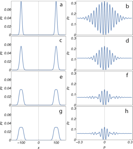
Notably, the non-ideal amplification process for certain range of parameters produces a probability distribution (see FIG. 5(e,g)) which has similar top-flat shape with that of our heuristic model illustrated in FIG. 1.
According to FIG. 5, as we include the non-ideal terms in the ideal phase-preserving linear amplifier, the interference effects vanish gradually. This also can be verified, using a quantitative measure of macroscopicity. Lee and Jeong introduced a general and inclusive measure of macroscopicity in the phase space as [47]

S(\rho)\!=\!\frac{\pi^{M}}{2}\!\int\!d^{2}\alpha W(\alpha)\sum_{m=1}^{M}\big[-\frac{\partial^{2}}{\partial\alpha_{m}\partial\alpha^{\ast}_{m}}-1\big]W(\alpha),

(14)

where $W(\alpha)$ is the Wigner function of the state and $M$ is the number of modes. The measure $S(\rho)$ was plotted for amplified coherent states with the first term, with first two terms and with first three terms in FIG. 6.

As we expected, this shows that with a large gain $g$ , as we include the non-ideal terms in the ideal amplifier, the probability of macroscopic quantum superpositions decreases.
To ensure that the non-ideal linear amplifier has a non-thermal effect, we compare the interference fringes appeared in the high-temperature thermal coherent state with those of a non-ideal amplified coherent state with equal purity, ${\rm Tr}(\rho_{th}^{2})={\rm Tr}(\{\varepsilon(\rho_{\alpha};g)\}^{2})$ . For a thermal coherent state with $v=d=100$ , the amplifier gain $g$ of the corresponding amplified coherent state with the first term, the first two terms and the first three terms are $7.10$ , $5.28$ and $4.56$ , respectively. For a fixed purity, the interference fringes for an amplifier with the corresponding terms were plotted in FIG. 7. The suppression of interference shows that including non-ideal terms has a non-thermal effect. The inclusion of many of terms in the actual detector can vanish the interference.

V Discussion & concluding remarks

It is of significance to come up with a form of quantum state representing the state of a macroscopic system, and resolving the problem of basis ambiguity, without necessarily invoking the entanglement with an environment or modifying the laws of quantum mechanics. That is why, we look at the amplifier, as it is supposed to describe the pointer’s state, and examine the basis ambiguity of the amplified state via a non-classical evolution sketched in FIG. 3. Our results show that an amplifier state can demonstrate a behavior which is not similar to that of a thermal coherent state when it is coupled to a microscopic state, yet having well-defined pointer position at the coarse-grained macroscopic scale. Nonetheless, we stress that to achieve a more conclusive result we need to examine a non-ideal amplifier state with realistic parameters. To our best knowledge, this is yet to be fully identified, and then this issue requires further research.

Acknowledgment

A. Asadian acknowledges Consolidator Grant 683107/TempoQ. *

Appendix A Resolution of Basis Ambiguity for Classical State

Here we prove that the classical state (3) is the same in all bases. In order to make more connection to the classical phase space description, we shift to the Wigner representation

	$\displaystyle W(\alpha)$	$\displaystyle=\frac{1}{\pi^{2}N}\sum_{j}\int d^{2}\beta\langle\alpha_{j}\|D(\beta)\|\alpha_{j}\rangle e^{-(\beta\alpha^{\ast}-\beta^{\ast}\alpha)}$
		$\displaystyle=\frac{2}{\pi N}\sum_{j}e^{-2\|\alpha-\alpha_{j}\|^{2}},$		(1)

where $D(\beta)$ is the displacement operator. As the summation is over all coherent states which lies in a single slot $\bar{\alpha}$ in the coarse-grained scale, we have

W(\alpha)=\delta(\alpha-\bar{\alpha}),

(2)

where $\bar{\alpha}$ is a coarse-grained phase amplitude which has classical dynamics. The mixed state corresponding to (1) would then be

\frac{1}{2}\delta(\alpha-\bar{\alpha})+\frac{1}{2}\delta(\alpha+\bar{\alpha}).

(3)

We may construct a new basis in terms of the old one as

	$\displaystyle\rho^{\pm}=\frac{4}{N}\sum_{j}^{N}$	$\displaystyle\Big(\|\alpha_{j}\rangle\langle\alpha_{j}\|+\|-\alpha_{j}\rangle\langle-\alpha_{j}\|$
		$\displaystyle\pm\|-\alpha_{j}\rangle\langle\alpha_{j}\|\pm\|\alpha_{j}\rangle\langle-\alpha_{j}\|\Big).$		(4)

The mixed state (3) can be equivalently decomposed in the new basis as

\frac{1}{2}\rho^{+}+\frac{1}{2}\rho^{-},

(5)

where the corresponding Wigner representation is

	$\displaystyle\frac{1}{2}\delta(\alpha-\bar{\alpha})$	$\displaystyle+\frac{1}{2}\delta(\alpha+\bar{\alpha})$
		$\displaystyle\pm\frac{2^{-2\|\alpha\|^{2}}}{\pi^{2}N}\sum_{i}\cos(4Im(\alpha_{i}^{\ast}\alpha)).$		(6)

The interference term is negligible, thus the decomposition in the new basis (6) is approximately the decomposition in the old basis (3). This means that the classicalized state of the pointer leads to a unique ensemble decomposition at coarse-grained scale. Therefore, $\delta(\alpha-\bar{\alpha})$ and $\delta(\alpha+\bar{\alpha})$ emerge dynamically as the unique coarse-grained or classical preferred basis.

References

[1] W. H. Zurek, Rev. Mod. Phys. 75, 715 (2003).
[2] M. Schlosshauer, Rev. Mod. Phys. 76, 1267 (2005).
[3] F. Shahandeh, F. Costa, A. P. Lund, and T. C. Ralph, arXiv preprint arXiv:1711.10498 (2017).
[4] J. S. Bell, Speakable and unspeakable in quantum mechanics (Cambridge University Press, 2004).
[5] N. P. Landsman, Handbook of the Philosophy of Science 2, 417 (2006).
[6] N. Bohr, Zeitschrift für Physik 13, 117 (1923).
[7] E. Schrödinger, Naturwissenschaften 14, 664 (1926).
[8] W. Schleich, M. Pernigo, and F. Le Kien, Phys. Rev. A 44, 2172 (1991).
[9] V. Bužek, A. Vidiella-Barranco, and P. L. Knight, Phys. Rev. A 45, 6570 (1992).
[10] C.-l. Chai, Phys. Rev. A 46, 7187 (1992).
[11] J. Janszky, P. Domokos, and P. Adam, Phys. Rev. A 48, 2213 (1993).
[12] J. Janszky, P. Domokos, S. Szabó, and P. Adam, Phys. Rev. A 51, 4191 (1995).
[13] S. Szabo, P. Adam, J. Janszky, and P. Domokos, Phys. Rev. A 53, 2698 (1996).
[14] H. M. Wiseman and J. A. Vaccaro, Phys. Rev. A 65, 043605 (2002a).
[15] H. M. Wiseman and J. A. Vaccaro, Phy. Rev. A 65, 043606 (2002b).
[16] L. M. Johansen, Phys. Let. A 329, 184 (2004a).
[17] B. S. Cirel’son, Lett. Math. Phys. 4, 93 (1980).
[18] F. Grosshans, G. Van Assche, J. Wenger, R. Brouri, N. J. Cerf, and P. Grangier, Nature 421, 238 (2003).
[19] L. M. Johansen, J. Opt. B: Quantum Semiclassical Opt. 6, L21 (2004b).
[20] H. Jeong and T. C. Ralph, Phys. Rev. Lett. 97, 100401 (2006).
[21] H. Jeong and T. C. Ralph, Phys. Rev. A 76, 042103 (2007).
[22] S.-B. Zheng, Phys. Rev. A 75, 032114 (2007).
[23] H. Jeong, J. Lee, and H. Nha, J. Opt. Soc. Am. B 25, 1025 (2008).
[24] A. Asadian, C. Brukner, and P. Rabl, Phys. Rev. Lett. 112, 190402 (2014).
[25] S. Machida and M. Namiki, Prog. Theor. Phys. 63, 1457 (1980a).
[26] S. Machida and M. Namiki, Prog. Theor. Phys. 63, 1833 (1980b).
[27] H. Araki, Progr. Theor. Phys. 64, 719 (1980).
[28] M. Namiki, H. Nakazato, and S. Pascazio, Decoherence and quantum measurements (World Scientific, 1998).
[29] W. Louisell, A. Yariv, and A. Siegman, Phys. Rev. 124, 1646 (1961).
[30] H. Heffner, Proceedings of the IRE 50, 1604 (1962).
[31] H. A. Haus and J. Mullen, Phys. Rev. 128, 2407 (1962).
[32] J. Gordon, L. Walker, and W. Louisell, Phys. Rev. 130, 806 (1963a).
[33] J. Gordon, W. H. Louisell, and L. Walker, Phys. Rev. 129, 481 (1963b).
[34] C. M. Caves, Phys. Rev. D 26, 1817 (1982).
[35] A. A. Clerk, M. H. Devoret, S. M. Girvin, F. Marquardt, and R. J. Schoelkopf, Rev. Mod. Phys. 82, 1155 (2010).
[36] V. B. Braginskii, Physics-Uspekhi 31, 836 (1988).
[37] C. M. Caves, K. S. Thorne, R. W. Drever, V. D. Sandberg, and M. Zimmermann, Rev. Mod. Phys. 52, 341 (1980).
[38] M. F. Bocko and R. Onofrio, Rev. Mod. Phys. 68, 755 (1996).
[39] C. M. Caves, J. Combes, Z. Jiang, and S. Pandey, Phys. Rev. A 86, 063802 (2012).
[40] A. Bassi and G. Ghirardi, Phys. Rep. 379, 257 (2003).
[41] J. Kofler and C. Brukner, Phys. Rev. Lett. 99, 180403 (2007).
[42] Q. Zhuang, T. Schuster, B. Yoshida, and N. Y. Yao, arXiv preprint arXiv:1902.04076 (2019).
[43] M. A. Rossi, C. Foti, A. Cuccoli, J. Trapani, P. Verrucchi, and M. G. Paris, Phys. Rev. A 96, 032116 (2017).
[44] B. Mollow and R. Glauber, Phys. Rev. 160, 1076 (1967a).
[45] B. R. Mollow and R. J. Glauber, Phys. Rev. 160, 1097 (1967b).
[46] M. Collett and D. Walls, Phys. Rev. Lett. 61, 2442 (1988).
[47] C.-W. Lee and H. Jeong, Phys. Rev. Lett. 106, 220401 (2011).

		$\displaystyle U_{\pi}\Big(\|{+}\rangle\!\langle{+}\|\otimes\varepsilon(\rho_{\alpha};g)\Big)U_{\pi}^{\dagger}$		(10)
		$\displaystyle=\|{+}\rangle\!\langle{+}\|\otimes E_{+}\varepsilon(\rho_{\alpha};g)E_{+}^{\dagger}+\|{-}\rangle\!\langle{-}\|\otimes E_{-}\varepsilon(\rho_{\alpha};g)E_{-}^{\dagger}$
		$\displaystyle+\|{+}\rangle\langle{-}\|\otimes E_{+}\varepsilon(\rho_{\alpha};g)E_{-}^{\dagger}+\|{-}\rangle\langle{+}\|\otimes E_{-}\varepsilon(\rho_{\alpha};g)E_{+}^{\dagger}.$