Hilbert Space Multi-dimensional Modeling

The following question can be asked about Table 1: Does a single $4-way$ joint probability distribution exist that can reproduce Table 1? The $4-way$ joint probability distribution is defined by $4$ binary random variables $(A,H,I,U)$ that generate $16$ latent joint probabilities that sum to one: $\pi(A=w\cap H=x\cap I=y\cap U=z),$ where, for example, $A$ is a random variable with values $w=1$ for yes and $w=0$ for no, and similar definitions hold for the other three random variables. For example, the relative frequency, $p(YN|AI),$ of YN in the context of the pair AI is predicted by the marginal $\pi(A=1,I=0)=\sum_{x}\sum_{z}\pi(A=1\cap H=x\cap I=0\cap U=z).$ Note that this $4-way$ joint distribution is completely general (non-parametric), because no conditional independence or parametric distribution assumptions are imposed.

The answer to the above question is negative: There is no single $4-way$ joint distribution that can reproduce Table 1. First of all, the $4-way$ distribution requires the marginal distribution of a single random variable to be invariant across contexts. This requirement fails. For example, the marginal probability of yes to random variable $I$ is not invariant: $p(YY|IU)+p(YN|IU)=.355$ which differs from $p(YY|UI)+p(NY|UI)=.420$. Table 1 contains other examples of violations of marginal invariance, depending on whether the attribute appeared first or second. The latter fact brings up a second problem: the order that questions are asked changes the $2-way$ distributions for some pairs. For example, the distribution for the context AH is not the same as the distribution for the context HA, and an order effect also occurs for the two contexts UI and IU. Order effects violate the commutative property required by the joint probability model: in particular, $\pi(A=w\cap H=x)=\pi(H=x\cap A=w),$ and $\pi(I=y\cap U=z)=\pi(U=z\cap I=y),$

It is interesting to notice that in this example, both marginal invariance and commutativity (no order effects) are satisfied by the four contexts AI, AU, HI, HU. Suppose we restrict our question to only these four tables, can a $4-way$ joint distribution reproduce these $4$ tables? Surprisingly, the answer is still negative. These $4$ tables violate a consistency requirement of a single $p-way$ joint distribution, called the Clauser, Horne, Shimony, and Holt (CHSH) inequality [11, 20, for applications in psychology, see].³³ 3 The CHSH inequality is closely related to the Bell inequality, and the latter was derived for the Bohm experiment using a pair of entangled spin $\frac{1}{2}$ photons, which was used to test the famous Einstein Podolsky Rosen (EPR) paradox. There are different ways to derive the CHSH inequality, and we follow the derivation by Fine [23]. The CHSH inequality implies the following restriction on the joint probabilities required by the $4-way$ joint probability model: $-1\leq CHSH\leq 2$, where

and, for example, $E(A\cdot I)=\pi(A=1\cap I=1)$ is the expectation of the product of the two random variables, $A,I.$ If we set $\pi(A=1\cap I=1)=p(YY|AI),$ $\pi(H=1\cap I=1)=p(YY|HI),$ $\pi(H=1\cap U=1)=p(YY|HU),$ $\pi(A=1\cap U=1)=p(YY|AU)$ from Table 1, then the CHSH value computed from Table 1 equals $CHSH=2.25$, which exceeds the bound required by the $4-way$ joint probability model. The CHSH is only one of a number of constraints that are required for a single joint distribution to reproduce a collection of contingency tables. Another inequality applies to $3-way$ joint distributions [44, 36]. Dzhafarov and Kujala [20] derive and provide a general summary of all these linear constraints required for a single joint distribution to reproduce a collection of contingency tables.

Suppose the data in Table 1 are based on a sample of $N=100$ independent observations for each $2\times 2$ table. Then it is unclear whether the violations of the $4-way$ joint probability distribution, described above, are statistically significant. To address this issue, we propose the following general method: We compare the $4-way$ joint probability model to a saturated model.⁴⁴ 4 This is what Dzhafarov and Kujala 21 call the all possible couplings model. The saturated model simply assumes that we have $8$ independent $2-way$ tables, and each table has $4$ probabilities that sum to one. The $4-way$ joint probability model has $15$ free parameters, because the 16 joint probabilities are constrained to sum to one. The saturated model has $8\times 3=24$ parameters, because the probabilities sum to one within each table. The $4-way$ joint probability model is nested within the saturated model, and the difference in number of parameters equals $df=24-15=9.$ Maximum likelihood methods can be used to estimate the parameters of each model, and $G^{2}=-2\times loglikelihood$ can be determined for each model. Then a likelihood ratio (i.e., chi-square difference) test can be used to compare models. Using this method with $N=100$ observations per table produces a chi-square difference equal to $G_{diff}^{2}=G_{joint}^{2}-G_{sat}^{2}=18.04$, which is a statistically significant difference with $p=.031$. Therefore, using this classical statistical test, the joint probability model is rejected. Note that this is a non-parametric test that requires no conditional independence or parametric distribution assumptions.

The above non-parametric method for testing a single $4-way$ joint distribution model can be generalized and applied to $p-way$ joint distributions as long as there is a sufficient number of tables that allow the saturated model to have more parameters than the joint distribution model. For example, if only the four $2\times 2$ tables (AI,AU,HI,HU) are included in the design, then the saturated model has only $4\times 3=12$ parameters, which is fewer than the $4-way$ joint distribution model (see, e.g., Bruza et al. 11).⁵⁵ 5 Nevertheless, $G_{diff}^{2}=2.56$ after fitting the $4-way$ model to Table 1, which reflects the violation of the CHSH inequality. However, if four $1-way$ tables, produced by measuring each attribute alone, are included into the design to form a collection of 8 tables (A,H,I,U, AI,AU,HI, HU), then the saturated model has $16$ parameters, which leaves $df=1$ for testing the joint probability model. It is worth nothing that the number of parameters in the joint probability model grows exponentially with the number of random variables, which makes it necessary to impose restrictions (e.g., using Bayesian networks or parametric distributional assumptions) to form testable models.

Including $1-way$ tables into the design provides direct tests of the marginal invariance assumption of the joint distribution model. For example, suppose attributes A,B are measured by binary choices, and the design included the three tables (A,B,AB). This simple design provides $2$ $df^{\prime}s$ for testing the joint distribution model (see, e.g., Wang and Busemeyer 52). Alternatively, including different orders of presentation provides direct tests of commutativity. For example, if attributes A,B are measured on $9$-point scales, and the design includes both $2-way$ tables (AB,BA), then $df=80$ for testing the joint probability model (see, e.g., Wang and Busemeyer 53).

On the one hand, an advantage of this non-parametric statistical test of the joint distribution model is that it tests all of the constraints imposed by the joint distribution model (including marginal invariance, absence of order effects, CHSH inequality, and others) with a single test. On the other hand, it does not isolate the particular property that is violated. We have developed more specific log likelihood statistical tests that are designed to test a particular property (e.g., a test of order effects versus a test of marginal invariance), but these additional tests are not described in detail here.

The commutative property has been tested by using the pair of tables (AB,BA) that vary question order. It has long been known that question order effects commonly occur with human judgments [46, 43]. Recently, quantum models have provided good accounts for these effects [51, 55, 53]. The marginal invariance assumption has been tested by using a design with two tables (A,BA). These are also called tests of the law of total probability, or tests for interference effects. Several experiments have been conducted that demonstrate violations of marginal invariance [13, 18, 15, 33, 50, 52]. A number of experiments have been conducted to test the CHSH or similar inequalities required by a single joint distribution applied to a collection of several $2\times 2$ tables [11, 4, 7, 26]. Although violations of the required inequalities were reported in the experiments testing the CHSH inequality, they were confounded with violations of marginal invariance [22]. It remains to be found out whether or not human judgments produce violations of the CHSH inequality in the absence of violations of order effects and marginal invariance [22].

It is helpful to introduce quantum probability theory by comparing it with classical probability theory.⁶⁶ 6 See Busemeyer and Bruza [12], Haven and Khrennikov [29], Khrennikov [31], van Rijsbergen [48] for introductions to quantum probability theory written for social and behavioral sciences. Although both classical and quantum theories are applicable to infinite spaces, for simplicity, we limit this presentation to finite spaces.

Suppose we have $p$ variables $(Y_{i},i=1,\cdots,p)$ and each variable, such as $Y_{i}$, produces one of a finite set of $n_{i}$ values when measured. In classical theory, variable $Y_{i}$ is called a random variable, and in quantum theory, $Y_{i}$ is called an observable. The measurement outcome generated by measuring one of the $p$ variables produces an event. For example, if variable $Y_{1}$ is measured and it produces the value $y_{i}$, then we observe the event $(Y_{1}=y_{i})$.

Classical theory begins with a universal set $\Omega$ containing all events, which is called the sample space; and quantum theory replaces this with a vector space $\mathscr{H}$ containing all events, which is called the Hilbert space. Classical theory defines an event $A$ as a subset of the sample space, whereas quantum theory defines an event $A$ as a subspace of the Hilbert space. Each subspace, such as $A$, corresponds to a projector, denoted $P_{A}$ for subspace $A,$ which projects vectors into the subspace. The change from subsets to subspaces is where the logic of events differs between the two theories.

Classical theory assumes closure: If $A\in\Omega$ is an event, and $B\in\Omega$ is another event, then $A\cap B\in\Omega$ is also an event in the sample space. By definition of intersection, the classical event $A\cap B$ is commutative $A\cap B=B\cap A$. In quantum theory, the events $A\in\mathscr{H}$, $B\in\mathscr{H}$ may not be commutative, and if they are not, then the conjunction does not exist, and closure does not hold. Instead, quantum theory uses the more general concept of a sequence of events.

In quantum theory, a sequence of events, such as $A$ and then $B$, denoted $AB$, is represented by the sequence of projectors $P_{B}P_{A}$. If the projectors commute, $P_{A}P_{B}=P_{B}P_{A}$, then the product of the two projectors is a projector corresponding to the subspace $A\cap B$, that is, $P_{B}P_{A}=P(A\cap B)$; and the events A and B are said to be compatible. However, if the two projectors do not commute, $P_{B}P_{A}\neq P_{A}P_{B}$, then neither their product is a projector, and the events are incompatible.

Classical theory defines a set function $p$ that assigns probabilities to events, which is required to be an additive measure: $p(A)\geq 0,$ $p(\Omega)=1,$ and if $A\cap B=\oslash$, then $p(A\cup B)=p(A)+p(B)$. Quantum theory uses a unit length state vector, denoted $\left|\psi\right\rangle\in\mathscr{H}$, to assign probabilities to events as follows:⁷⁷ 7 A more general approach uses what is called a density operator rather than a pure state vector, but to keep ideas simple, we use the latter.

Quantum probabilities also satisfy an additive measure: $p(A)\geq 0,$ $p(\mathscr{H})=1,$ and if $P_{A}P_{B}=0,$ then $p(A\vee B)=p(A)+p(B)$. In fact, Equation 2 is the unique way to assign probabilities to subspaces that form an additive measure for dimensions greater than 2 [24].

According to classical theory, if an event $A$ is an observed fact, then the conditional probability of event $B$ is defined as

and so the joint probability of $A\cap B$ equals $p(A\cap B)=p(A)\cdot p(B|A).$ The corresponding definition in quantum theory is

and so the probability of the sequence $AB$ equals $p(AB)=p(A)\cdot p(B|A)=\left\|P_{B}P_{A}\left|\psi\right\rangle\right\|^{2}.$ The commutative property of classical probability requires that $p(A)\cdot p(B|A)=p(B)\cdot p(A|B)$, but this commutative property does not hold for quantum theory so that $p(A)\cdot p(B|A)\neq p(B)\cdot p(A|B)$ occurs when events are incompatible.

Extensions to sequences with more than two events follows the same principles for both classical and quantum theories. The probability of the joint event $\left(A\cap B\right)\cap C$ equals $p(\left(A\cap B\right)\cap C)$ for classical theory, and the probability of the sequence $(AB)C$ equals $\left\|P_{C}\left(P_{B}P_{A}\right)\left|\psi\right\rangle\right\|^{2}$ for quantum theory.

This section describes a general way to construct the projectors for events in the Hilbert space, and to formally describe the conditions that produce incompatibility. This section is somewhat abstract and technical, and a concrete application is provided in the next section where we build a simple model for Table 1. In the following, $\left|V\right\rangle$ denotes a vector in the Hilbert space, $\left\langle V|W\right\rangle$ denotes an inner product, $\left|V\right\rangle\left\langle V\right|$ denotes an outer product, and $P^{\dagger}$ denotes a Hermitian transpose.

In general, a projector, denoted $P$, operating in an $N-$dimensional Hilbert space $\mathscr{H}$, is defined by the two properties $P=P^{\dagger}=P^{2}$. By the first property, $P$ is Hermitian, and so it can be decomposed into $N$ orthonormal eigenvectors; by the second property, $P$ has only two eigenvalues, which are simply $(0,1)$ [28]. Define $\left|V_{j}\right\rangle,j=1,\cdots,N$ as the set of $N$ orthonormal eigenvectors of $P$. The projector $P$ can be expressed in terms of the eigenvectors as follows

where the outer product, $\left|V_{j}\right\rangle\left\langle V_{j}\right|$, is the projector that projects into the ray spanned by eigenvector $\left|V_{j}\right\rangle$, and $\lambda_{j}=1$ if $\left|V_{j}\right\rangle$ corresponds to an eigenvalue of 1, and $\lambda_{j}=0$ if $\left|V_{j}\right\rangle$ corresponds to an eigenvalue of $0.$ These $N$ eigenvectors form an orthonormal basis that spans the Hilbert space. Every vector, such as $\left|\psi\right\rangle\in\mathscr{H}$ can be expressed as a linear combination of these basis (eigen) vectors

If two projectors, $P_{A},P_{B}$ share all of the same eigenvectors, then they commute [28]. In other words, two events $A,B$ are compatible if they are described in terms of the same basis. If the two projectors do not share all of the same eigenvectors, then they do not commute, and the events $A,B$ are described by two different bases. They are incompatible, and must be evaluated sequentially, because one needs to change from one basis to evaluate the first event, to another basis to evaluate the second event, making them incompatible.

Define $\left|V_{j}\right\rangle,j=1,\cdots,N$ as the basis used to describe event $A,$ and define $\left|W_{j}\right\rangle,j=1,\cdots,N$ as the basis used to describe event $B.$ We can change from one basis to another by a unitary transformation (a “rotation” in Hilbert space)

where $U$ is defined by $U^{\dagger}U=I$, that is, $U$ is an isometric transformation that preserves inner products [28]. Therefore, the projector for event $B$ can be re-expressed in terms of the event $A$ basis $\left|V_{j}\right\rangle,j=1,\cdots,N$ as follows

According to Equation 5, the unitary transformation $U$ represents the transitions from state $\left|W_{i}\right\rangle$ to state $\left|V_{j}\right\rangle$ by the inner product $\left\langle V_{j}|W_{i}\right\rangle$.

So far, we have presented a general method for building the projectors by defining a basis for the vector space and by transforming from one basis to another using unitary transformation. Then the next question is how to build the unitary transformation? In general, any unitary transformation can be built from a Hermitian operator $H$ as follows (Halmos, 1993):

The right hand side is exponential function of the Hermitian operator $H$ (see appendix for details).

In summary, the HSM program selects a Hermitian operator $H$ for Equation 7, and then uses the Hermitian operator to build the unitary operator $U$ which provides the relation between projectors $P_{A}$ and $P_{B}$ for incompatible events. The beauty of using a vector space is that it provides an infinite number of ways to generate incompatible variables by unitary “rotation,” and yet remain within the same $N-$dimensional space. This is how an HSM model maintains a low dimensional representation even when there are a large number of variables.

This section describes how we construct a Hilbert space to represent the $p$ variables. This construction depends on the compatibility relations between the variables. For this section, we need to use the Kronecker (tensor) product between two matrices, denoted as $P\otimes Q$ (see the Appendix for a brief review).

To begin building the Hilbert space, suppose we measure a single variable, say $Y_{1}$, that can produce $n_{1}$ values corresponding to the mutually exclusive and exhaustive set of events $(Y_{1}=y_{i}),i=1,\cdots n_{1}.$ To represent these events in a Hilbert space, we partition the space into $n_{1}$ orthogonal subspaces. Each subspace, such as $(Y_{1}=y_{i})$, corresponds to a projector $P(Y_{1}=y_{i}).$ The projectors for all of the events are pairwise orthogonal, $P(Y_{1}=y_{i})P(Y_{1}=y_{j})=\mathbf{0}$, and complete, $\sum_{i}P(Y_{1}=y_{i})=\mathbf{I}$ (where $\mathbf{I}$ is the identity that projects onto the entire Hilbert space). These $n_{1}$ events are all compatible, and the projectors are all commutative, because they are all orthogonal to each other. Each projector generates $N_{1}\geq n_{1}$ eigenvectors, and the projectors all share the same eigenvectors, but with different eigenvalues. These $N_{1}$ eigenvectors provide the basis for spanning a $N_{1}-$dimensional Hilbert space, $\mathscr{H}_{N_{1}}$.

Continuing with the case of a single variable represented by the Hilbert space $\mathscr{H}_{N_{1}}$ , we can express each vector $\left|\phi\right\rangle\mathscr{\in H}_{N_{1}}$ in terms of its coordinates with respect to the eigenvectors of $P(Y_{1}=y_{i})$ by using Equation 4. Using this basis, the coordinate representation of each projector, say $P(Y_{1}=y_{i})$ is simply an $N_{1}\times N_{1}$ diagonal matrix, $M_{1}(i)$ with ones located in the rows corresponding to basis vectors that have an eigenvalue of one associated with the projector $P(Y_{1}=y_{i})$, and zeros otherwise. The coordinate representation of $\left|\psi\right\rangle$ with respect to this basis is a $N_{1}\times 1$ column matrix $\psi$ with coordinate $\psi_{i}$ in row $i,$ which satisfies $\psi^{\dagger}\psi=1$. Then the probability distribution over the values of $Y_{1}$ for $i=1,\cdots,n_{1}$ is given by

There is little difference between classical and quantum probability at this point.

Next suppose we measure two variables, $Y_{1}$ with $n_{1}$ values and $Y_{2}$ with $n_{2}$ values, with $n_{1}\geq n_{2}$. If these two variables are compatible, then the joint event $(Y_{1}=y_{i}\cap Y_{2}=y_{j})$ is well defined for all pairs of values. Therefore the Hilbert space is partitioned into $n_{1}\cdot n_{2}$ orthogonal subspaces. Each subspace corresponds to a projector $P(Y_{2}=y_{j})P(Y_{1}=y_{i})=P(Y_{1}=y_{i})P(Y_{2}=y_{j})=P(Y_{1}=y_{i}\cap Y_{2}=y_{j})$. These projectors are pairwise orthogonal and complete, and every pair of projectors is commutative. Each projector shares $(N_{1}\cdot N_{2})\geq(n_{1}\cdot n_{2})$ eigenvectors, but with different eigenvalues, to span a Hilbert space $\mathscr{H}_{N_{1}\cdot N_{2}}$. Using this basis, the projector $P(Y_{1}=y_{i})$ is represented by the Kronecker product $M_{1}(i)\otimes I_{N_{2}}$, where $I_{N_{2}}$ is an $N_{2}\times N_{2}$ identity matrix. The projector $P(Y_{2}=y_{j})$ is represented by the matrix Kronecker product $I_{N_{1}}\otimes M{}_{2}(j)$. Then $P(Y_{2}=y_{j})P(Y_{1}=y_{i})=P(Y_{1}=y_{i}\cap Y_{2}=y_{j})$ is represented by the product $\left(M_{1}(i)\otimes I_{N_{2}}\right)\cdot\left(I_{N_{1}}\otimes M{}_{2}(j)\right)=M_{1}(i)\otimes M{}_{2}(j)$, which is simply a diagonal matrix with ones located in the rows corresponding to $(Y_{1}=y_{i}\cap Y_{2}=y_{j})$ and zeros otherwise. The coordinate representation of $\left|\psi\right\rangle$ with respect to this basis is a $\left(N_{1}\cdot N_{2}\right)\times 1$ column matrix, $\left(\psi,\psi^{\dagger}\psi=1\right)$, with coordinate $\psi_{ij}$ in row $n_{2}\cdot(i-1)+j$. Then the joint probability for a pair of values equals

There is still little difference between the classical and quantum theories at this point. Adding variables increases the dimensionality of the space, just like it does with a Bayesian model.

Now suppose that variables $Y_{1}$ (with $n_{1}$ values) and $Y_{2}$ (with $n_{2}\leq n_{1}$ values) are incompatible. In this case, we cannot define the joint occurrence of two events $(Y_{1}=y_{i}\cap Y_{2}=y_{j})$, and we can only represent a sequence of two single events, e.g., $\left(Y_{1}=y_{i}\right)$ and then $\left(Y_{2}=y_{j}\right)$ by the sequence of projectors $P(Y_{2}=y_{j})P(Y_{1}=y_{i})$. As before, we define $P(Y_{1}=y_{i})$ as the projector for the event $\left(Y_{1}=y_{i}\right),$ and likewise, we define $P(Y_{2}=y_{j})$ as projector for the event $\left(Y_{2}=y_{j}\right).$ Both projectors are represented with a Hilbert space, $\mathscr{H}_{N_{1}}$, of dimension $N_{1}\geq n_{1}$. We can choose to express each vector $\left|\phi\right\rangle\mathscr{\in H}_{N_{1}}$ in terms of the coordinates with respect to the eigenvectors of $P(Y_{1}=y_{i})$ by using Equation 4. Using this basis, the coordinate representation of projector $P(Y_{1}=y_{i})$ is simply an $N_{1}\times N_{1}$ diagonal matrix, $M_{1}(i)$ with ones located in the rows corresponding to basis vectors that have an eigenvalue of one associated with this projector, and zeros otherwise. Using Equation 5, the projector $P(Y_{2}=y_{j})$ can be expressed in terms of the $P(Y_{1}=y_{i})$ basis by a unitary matrix, $U$. Then the matrix representation of $P(Y_{2}=y_{j})$ is $\left(U\cdot M{}_{1}(j)\cdot U^{\dagger}\right)$. Finally, the coordinate representation of the state vector $\left|\psi\right\rangle$ with respect to the $Y_{1}$ basis is a $N_{1}\times 1$ column matrix $\psi$. The probability of the sequence of events $\left(Y_{1}=y_{i}\right)$ and then $\left(Y_{2}=y_{j}\right)$ equals

This is where a key difference between the classical and quantum theories occurs. Note that, unlike a Bayesian model, adding variable $Y_{2}$ does not increase the dimensionality of the space.

Finally suppose that we measure three variables, $Y_{1}$ with $n_{1}$ values, $Y_{2}$ with $n_{2}$ values, and $Y_{3}$ with $n_{3}$ values. Suppose $Y_{1}$ is compatible with $Y_{2}$ and $Y_{2}$ is compatible with $Y_{3}$ but $Y_{1}$ is incompatible with $Y_{3}$. In this case, we can partition the Hilbert space using projectors $P(Y_{1}=y_{i}\cap Y_{2}=y_{j}),i=1,\cdots n_{1},j=1,\cdots n_{2}$, which are pairwise orthogonal and complete, and every pair of these projectors is commutative. Using the eigenvectors of these projectors as the basis, the projector $P(Y_{1}=y_{i})$ is represented by the Kronecker product $M_{1}(i)\otimes I_{N_{2}}$, and the projector $P(Y_{2}=y_{j})$ is represented by the Kronecker product $I_{N_{1}}\otimes M{}_{2}(j)$. Using a unitary transformation, $U,$ the matrix representation of the projector $P(Y_{3}=y_{k})$ is given $\left(U\cdot M_{1}(k)\cdot U^{\dagger}\right)\otimes I_{N_{2}}$. Then, the probability of the two compatible events $\left(Y_{1}=y_{i}\right)$ and$\left(Y_{2}=y_{j}\right)$ equals

the probability of the two compatible events $\left(Y_{2}=y_{i}\right)$ and $\left(Y_{3}=y_{j}\right)$ equals

and the probability of the sequence of two incompatible events $\left(Y_{1}=y_{i}\right)$ and then $\left(Y_{3}=y_{k}\right)$ equals

The methods described above generalize in a fairly straightforward manner for more variables. Note that when variables are compatible, quantum probability theory works like classical probability theory, and the Hilbert space dimensionality increases exponentially as the number of compatible variables increases. However, when variables are incompatible, it is unlike classical probability theory, and the Hilbert space dimensionality remains constant as the number of incompatible variables increases. In short, incompatibility–a central concept in quantum theory and its application to psychology [39, 56]–produces simplification by rotating the basis to generate variables rather than adding new dimensions.

An HSM model is built using the following programatic steps. All of these steps are illustrated in the next section with a concrete application to the artificial data set.

First, the researcher needs to determine which variables or attributes are commutative, and which are not. Referring to our artificial data set, we need to determine, for example, whether the attributes $A$ and $H$ commute or not. Recall that if they are compatible, then they can be defined simultaneously, and sequence does not matter; but if they are incompatible, they must be evaluated sequentially, because one needs to change from one basis to another basis for evaluating the sequence. One way to determine this is to observe whether or not a pair of variables produce order effects. Alternatively, one can statistically compare competing models with different hypothesized compatibility relations.

Second, the dimension $N$ of the Hilbert space is determined. This depends first of all on the assumed compatibility relations. Given the compatibility relations, an HSM modeling procedure can begin with the lowest possible dimension, and only increase the dimension as required by model comparisons that favor a higher dimension.

Third, a basis is selected for representing the coordinates of the state vector $\left|\psi\right\rangle$ in terms of combinations of compatible variables. Once a basis is chosen, the coordinates of the state vector, represented by the $N\times 1$ column matrix $\psi$, can be estimated from the data. In general, each coordinate can be complex, containing a magnitude and a phase. Therefore, if the dimension equals $N,$ then the initial state requires $2\cdot N$ parameters. However, the initial state must satisfy the unit length constraint $\psi^{\dagger}\psi=1$, which constrains one magnitude. Also one phase can be arbitrarily fixed without any effect on the choice probability. In sum, only $2\cdot(N-1)$ parameters are estimated from the data.

Fourth, the projectors from unitary transformations are built, and the latter are obtained by selecting a Hermitian operator used in Equation 7. In general, the Hermitian matrix has $N$ diagonal entries that are real, and $N\cdot(N-1)/2$ off diagonal entries, that can be complex. However, adding a constant to all the diagonal entries has no effect on the choice probabilities, and so one diagonal entry can be set to a fixed value. In sum, only $\left(N^{2}-1\right)$ parameters are estimated for each Hermitian matrix.

Fifth, using quantum probability rules, the probability of a sequence of measurements is computed. Using the predicted probabilities, the model computes the log likelihood of the data given the model. The parameters for the initial state and the Hermitian operators are estimated from the data using maximum likelihood, and the model computes $G^{2}=-2\cdot loglikelihood$ statistics for model comparison.¹⁰¹⁰ 10 Currently, we use a particle swarm method to estimate parameters in order to avoid local minimum. The number of model parameters is determined by the number of parameters used to build the initial state vector plus the number of parameters used to estimate the Hermitian operators used in Equation 7.

Sixth, the fit of the model returns parameters for the initial state that can be used to describe the probability distribution over a variable as if it were measured alone (free of context of other variables), and also the parameters of the unitary transformations that describe the relations between incompatible variables.

Seventh, an HSM model allows many opportunities for very strong generalization tests of the model. For example, if there are three variables, and two of them are incompatible, then after estimating the model parameters from an HSM model for a collection of $2\times 2$ tables, the same model and parameters can be used to make new predictions for new tables that were not included in the original design, such as smaller $1-way$ tables or larger $3-way$ tables.

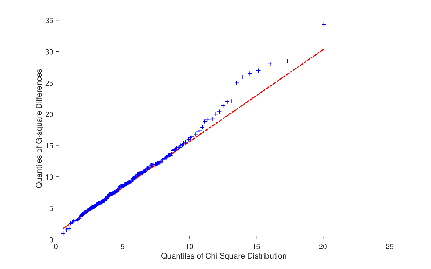
Each individual produced a table in the same form as Table 4, but with 16 observations per $2\times 2$ table (192 observations in total for both types of stimuli). Recall that the joint probability model states that the 6 rows of $2\times 2$ tables are produced by a joint distribution, $\pi(P=w\cap B=x\cap I=y\cap L=z)$ where $w=0,1,$ $x=0,1$, $y=0,1$ and $z=0,1$, that has $16-1=15$ free parameters per stimulus type or $30$ parameters altogether. The saturated model requires $3$ parameters for each $2\times 2$ table, producing a total of $18$ parameters per stimulus type or $36$ parameters altogether. Using maximum likelihood estimation for each person, we computed the $G_{sat}^{2}$ and $G_{joint}^{2}$ for each person. A quantile-quantile plot of the observed $G^{2}$ differences, $G_{diff}^{2}=G_{joint}^{2}-G_{sat}^{2}$ versus the $\chi^{2}$ predicted by the null hypothesis is shown in Figure 1. As can be seen in Figure 1, the observed $G_{diff}^{2}$ exceeds the expected for large values of the predicted chi-square. We computed a lack of fit from the null chi-square distribution by comparing the observed versus expected frequencies using categories defined by cutoffs [0, 5, 10, 35]. The expected frequencies were $[84,77,23]$ but the observed frequencies were $[48,75,61]$, and the difference is statistically significant ($\chi^{2}(2)=78.84$). We conclude that the $4-way$ joint probability model systematically deviates from the observed results for a substantial number of individuals.

Any Bayesian network model, based on the four random variables, P,B,I and L, is a special case of the $4-way$ joint probability model, which implies that there is also some systematic deviation from any Bayes net type of model. However, there may also be systematic deviations from a HSM model. Therefore, it is important to compare the fits of Bayes net versus HSM models. Because they two types of models are non-nested, we performed comparisons at the individual level using the Bayesian information criterion $BIC_{Model}=G_{Model}^{2}+p\cdot ln(192)$, where $G_{Model}^{2}=-2\cdot loglikelihood$, and $p=$number of model parameters.

There are a large number of possible Bayes net type of models that one can construct for this application. We chose the following model because (a) it is simple and (b) it makes assumptions that match design of the stimuli and responses to the stimuli for this experiment. We note, however, that our conclusions are restricted to these particular models, and there may be other Bayes net models that perform better than the one here.

For the Bayes net type of model, we assumed that the two attributes, Informative (I) and Believable (B), are exogenous factors determined by the type of PSA’s. Therefore, each type of stimulus produced a $2-way$ joint distribution with four joint probabilities $\pi(I=x\cap B=y|stimulus),$ $x=0,1,$ $y=0,1$, and there are $2$ types of stimuli. This produces $(4-1)\cdot 2=6$ parameters per stimulus type. Next we assumed that the response to attributes Persuasive (P) and Likable (L) depended on the stimulus attributes I and B, which was represented by the conditional probabilities $\pi(P=w\cap L=z|I=x\cap B=y)$, for $w=0,1$ and $z=0,1$. However, this model produces the same number ($15\cdot 2=30$) of parameters as the $4-way$ joint probability model. To simplify the model, we assumed independence, so that $\pi(P=w\cap L=z|I=x\cap B=y)=\pi(P=w|I=x\cap B=y)\cdot\pi(L=z|I=x\cap B=y)$. We also assumed that the two conditionals, $\pi(P=w|I=x\cap B=y)$ and $\pi(L=z|I=x\cap B=y)$, did not depend on the stimulus type. Therefore, each of the two conditionals produces four parameters. Altogether, this model entails $(4-1)\cdot 2+\left(4\cdot 2\right)=14$ parameters.

The same simple HSM model used to fit the artificial data in the previous section was applied to the real data from our experiment. First, we assumed that the attributes, Believable (B) and Informative (I) are compatible, which means we can think of these two attributes at the same time and the order of measuring the two attributes does not matter. This is consistent with the lack of effect of the order effects of the two attributes in the aggregated data. Second, we assumed that Persuasive (P) is a rotation of Believable, and Likable (L) is a rotation of Informative. In other words, B,P were assumed to be incompatible and so were I,L. This assumption was also consistent with order effects found at the aggregate level for these variables. For simplicity, we assumed that each joint event for a compatible pair, such as $(B=x\cap I=y)$, is represented by a single dimension. We chose to represent the initial state and projectors by the basis described by the B,I events $(B=x\cap I=y).$

To reduce the number of model parameters to a minimum, we restricted the coordinates of the initial state to be a real valued $4\times 1$ matrix $\psi$ with unit length $\psi^{\dagger}\psi=1$. The unitary matrix for rotating between the incompatible basis vectors was constructed using a single parameter as follows:

References

- [1] D. Aerts. Quantum structure in cognition. Journal of Mathematical Psychology, 53 (5):314–348, 2009.
- [2] D. Aerts and L. Gabora. A theory of concepts and their combinations ii: A hilbert space representation. Kybernetes, 34:192–221, 2005.
- [3] D. Aerts, J. Broekaert, and L. Gabora. A case for applying an abstracted quantum formalism to cognition. New Ideas in Psychology, 29:136–146, 2011.
- [4] D. Aerts, L. Gabora, and S. Sozzo. Concepts and their dynamics: A quantum - theoretic modeling of human thought. Topics in Cognitive Science, 5:737–773, 2013.
- [5] A. Agresti and M. Katera. Categorical data analysis. Springer, 2011.
- [6] C. J. Anderson. Analysis of multivariate frequency data by graphical models and generalizations of the multidimensional row-column association model. Psychological methods, 7(4):446–467, 2002.
- [7] Masanari Asano, Takahisa Hashimoto, Andrei Khrennikov, Masanori Ohya, and Yoshiharu Tanaka. Violation of contextual generalization of the leggett–garg inequality for recognition of ambiguous figures. Physica Scripta, 2014(T163):014006, 2014.
- [8] Masanari Asano, Irina Basieva, Andrei Khrennikov, Masanori Ohya, and Yoshiharu Tanaka. A quantum-like model of selection behavior. Journal of Mathematical Psychology, 2016.
- [9] Thomas Boyer-Kassem, Sébastien Duchêne, and Eric Guerci. Testing quantum-like models of judgment for question order effect. Mathematical Social Sciences, 80:33–46, 2016.
- [10] P. D. Bruza, Z. Wang, and J. R. Busemeyer. Quantum cognition: a new theoretical approach to psychology. Trends in cognitive sciences, 19(7):383–393, 2015a.
- [11] Peter D Bruza, Kirsty Kitto, Brentyn J Ramm, and Laurianne Sitbon. A probabilistic framework for analysing the compositionality of conceptual combinations. Journal of Mathematical Psychology, 67:26–38, 2015b.
- [12] J. R. Busemeyer and P. D. Bruza. Quantum models of cognition and decision. Cambirdge University Press, 2012.
- [13] J. R. Busemeyer, Z. Wang, and A. Lambert-Mogiliansky. Empirical comparison of markov and quantum models of decision making. Journal of Mathematical Psychology, 53 (5):423–433, 2009.
- [14] J. R. Busemeyer, E. M. Pothos, R. Franco, and J. S. Trueblood. A quantum theoretical explanation for probability judgment errors. Psychological Review, 118 (2):193–218, 2011.
- [15] E. Conte, A. Y. Khrennikov, O. Todarello, A. Federici, L. Mendolicchio, and J. P. Zbilut. Mental states follow quantum mechanics during perception and cognition of ambiguous figures. Open Systems and Information Dynamics, 16:1–17, 2009.
- [16] Adnan Darwiche. Modeling and reasoning with Bayesian networks. Cambridge University Press, 2009.
- [17] Kim De Roover, Eva Ceulemans, Marieke E Timmerman, Kristof Vansteelandt, Jeroen Stouten, and Patrick Onghena. Clusterwise simultaneous component analysis for analyzing structural differences in multivariate multiblock data. Psychological methods, 17(1):100–119, 2012.
- [18] G. M. Di Nunzio, P. Bruza, and L. Sitbon. Interference in Text Categorization Experiments, pages 22–33. Springer, 2014.
- [19] P. A. M. Dirac. The principles of quantum mechanics. Oxford University Press, 1930/1958.
- [20] E. Dzhafarov and J. V. Kujala. Selectivity in probabilistic causality: Where psychology runs into quantum physics. Journal of Mathematical Psychology, 56:54–63, 2012.
- [21] E. N. Dzhafarov and J. V. Kujala. All-possible-couplings approach to measuring probabilistic context. PloS one, 8(5):e61712, 2013.
- [22] Ehtibar N Dzhafarov, Ru Zhang, and Janne Kujala. Is there contextuality in behavioural and social systems? Phil. Trans. R. Soc. A, 374(2058):20150099, 2016.
- [23] A. Fine. Joint distrbutions, quantum correlations and commuting observables. Journal of Mathematical Physics, 23(7):1306–1310, 1982.
- [24] A. M. Gleason. Measures on the closed subspaces of a hilbert space. Journal of Mathematical Mechanics, 6:885–893, 1957.
- [25] P beim Graben and H. Atmanspacher. Complementarity in classical dynamical systems. Foundations of Physics, 36:291–306, 2006.
- [26] G. Gronchi and E. Strambini. Quantum cognition and bells inequality, a model for probabilistic judgment bias. Journal of Mathematical Psychology, 2016.
- [27] S. P. Gudder. Quantum Probability. Academic Press, 1988.
- [28] P. R. Halmos. Finite-Dimensional vector spaces. Springer Undergraduate Texts in Mathematics, 1993.
- [29] E. Haven and A. Khrennikov. Quantum social science. Cambirdge University Press, 2013.
- [30] Joel Huber, John W Payne, and Christopher Puto. Adding asymmetrically dominated alternatives: Violations of regularity and the similarity hypothesis. Journal of consumer research, 9(1):90–98, 1982.
- [31] A. Y. Khrennikov. Ubiquitous quantum structure: From Psychology to Finance. Springer, 2010.
- [32] A. N. Kolmogorov. Foundations of the theory of probability. N.Y.: Chelsea Publishing Co., 1933/1950.
- [33] P. D. Kvam, T. J. Pleskac, S. Yu, and J. R. Busemeyer. Interference effects of choice on confidence. , 112 (34). Proceedings of the National Academy of Science, 112 (34):10645–10650, 2015.
- [34] P. La Mura. Projective expected utility. Journal of Mathematical Psychology, 53 (5):408–414, 2009.
- [35] A. Lambert-Mogiliansky, S. Zamir, and H. Zwirn. Type indeterminacy: A model of the ’kt’ (kahneman-tversky)-man. Journal of Mathematical Psychology, 53 (5):349–361, 2009.
- [36] A. J. Leggett and A. Garg. Quantum mechanics versus macroscopic realism: Is the flux there when nobody looks. Physical Review Letters, 54:857–860, 1985.
- [37] John J McArdle, Kevin J Grimm, Fumiaki Hamagami, Ryan P Bowles, and William Meredith. Modeling life-span growth curves of cognition using longitudinal data with multiple samples and changing scales of measurement. Psychological methods, 14(2):126–149, 2009.
- [38] I Pitowski. Quantum probability, Quantum logic., volume 321 Lecture Notes in Physics. Springer, 1989.
- [39] Arkady Plotnitsky. Niels Bohr and complementarity: An introduction. Springer Science & Business Media, 2012.
- [40] E. M. Pothos and J. R. Busemeyer. A quantum probability model explanation for violations of ‘rational’ decision making. Proceedings of the Royal Society, B., 276 (1665):2171–2178, 2009.
- [41] E. M. Pothos and J. R. Busemeyer. Can quantum probability provide a new direction for cognitive modeling? Behavioral and Brain Sciences, 36:255–274, 2012.
- [42] E. M. Pothos, J. R. Busemeyer, and J. S. Trueblood. A quantum geometric model of similarity. Psychological Review, 120 (3):679–696, 2013.
- [43] H. Schuman and S. Presser. Questions and answers in attitude surveys: Experiments on question form, wording, and content. NY: Academic Press, 1981.
- [44] P. Suppes and M. Zanotti. When are probabilsitic explanations probable? Synthese, 48(191-199), 1981.
- [45] Patrick Suppes. Probability concepts in quantum mechanics. Philosophy of Science, 28(4):378–389, 1961.
- [46] R. Tourangeau, L. J. Rips, and K. A. Rasinski. The psychology of survey response. Cambridge University Press, 2000.
- [47] J. S. Trueblood and J. R. Busemeyer. A quantum probability account for order effects on inference. Cognitive Science, 35:1518–1552, 2010.
- [48] C.J. van Rijsbergen. The Geometry of Information Retrieval. Cambridge University Press, 2004.
- [49] J. Von Neumann. Mathematical Foundations of Quantum Theory. Princeton University Press, 1932/1955.
- [50] Benyou Wang, Peng Zhang, Jingfei Li, Dawei Song, Yuexian Hou, and Zhenguo Shang. Exploration of quantum interference in document relevance judgement discrepancy. Entropy, 18(4):144, 2016.
- [51] Z. Wang and J. R. Busemeyer. A quantum question order model supported by empirical tests of an a priori and precise prediction. Topics in Cognitive Science, 5(4):689–710, 2013.
- [52] Z. Wang and J. R. Busemeyer. Interference effecs of categorization on decision making. Cognition, 150:133–149, 2016a.
- [53] Z Wang and JR Busemeyer. Comparing quantum versus markov random walk models of judgements measured by rating scales. Phil. Trans. R. Soc. A, 374(2058):20150098, 2016b.
- [54] Z. Wang, J. R. Busemeyer, H. Atmanspacher, and E. M. Pothos. The potential of using quantum theory to build models of cognition. Topics in Cognitive Science, 5(4):672–688, 2013.
- [55] Z. Wang, T. Solloway, R. M. Shiffrin, and J. R. Busemeyer. Context effects produced by question orders reveal quantum nature of human judgments. Proceedings of the National Academy of Sciences of the USA, 111 (26):9431–9436, 2014.
- [56] Zheng Wang and Jerome Busemeyer. Reintroducing the concept of complementarity into psychology. Frontiers in psychology, 6(1822), 2015.
- [57] Forrest W Young. Multidimensional scaling: History, theory, and applications. Psychology Press, 2013.
- [58] V. I. Yukalov and D. Sornette. Decision theory with prospect interference and entanglement. Theory and Decision, 70:283–328, 2011.
7 Appendix
7.1 Matrix exponential function
Suppose is the matrix representation of a Hermitian operator. Then we can decompose into its orthonormal eigenvector matrix and its real eigenvalue diagonal matrix as follows: . The matrix exponential of is defined as
7.2 Kronecker product
Suppose is a matrix and is a matrix. Then the Kronecker product is a matrix defined by
For example,
The Kronecker product satisfies the following property (assuming the column dimension of matches the row dimension of and likewise for and
7.3 Parameters used to fit artificial data