A note on energy forms on fractal domains

Claire David

Sorbonne Universités, UPMC Univ Paris 06

CNRS, UMR 7598, Laboratoire Jacques-Louis Lions, 4, place Jussieu 75005, Paris, France

1 Introduction

In [1], [2], J. Kigami has laid the foundations of what is now known as analysis on fractals, by allowing the construction of an operator of the same nature of the Laplacian, defined locally, on graphs having a fractal character. The Sierpiński gasket stands out of the best known example. It has, since then, been taken up, developed and popularized by R. S. Strichartz [4], [20].

The Laplacian is obtained through a weak formulation, obtained by means of Dirichlet forms, built by induction on a sequence of graphs that converges towards the considered domain. It is these Dirichlet forms that enable one to obtain energy forms on this domain.

Yet, things are not that simple. If, for domains like the Sierpiński gasket, the Laplacian is obtained in a quite natural way, one must bear in mind that Dirichlet forms solely depend on the topology of the domain, and not of its geometry. Which means that, if one aims at building a Laplacian on a fractal domain, the topology of which is the same as, for instance, a line segment, one has to find a way of taking account a very specific geometry. We came across that problem in our work on the graph of the Weierstrass function [6]. The solution was thus to consider energy forms more sophisticated than classical ones, by means of normalization constants that could, not only bear the topology, but, also, the very specific geometry of, from now on, we will call ${\cal W}-$ curves.

It is interesting to note that such problems do not seem to arise so much in the existing literature. In a very general way, one may refer to [8], where the authors build an energy form on non-self similar closed fractal curves, by integrating the Lagrangian on this curve.

We presently aim at investigating the links between energy forms and geometry. We have chosen to consider fractal curves, specifically, the Sierpiński arrowhead curve, the limit of which is the Sierpiński gasket. Does one obtain the same Laplacian as for the triangle ? The question appears as worth to be investigated.

2 Framework of the study

We place ourselves, in the following, in the Euclidean plane of dimension 2, referred to a direct orthonormal frame. The usual Cartesian coordinates are $(x,y)$ .

Notation.

Given a point $X\,\in\,{\mathbb{R}}^{2}$ , we will denote by:

i.

${\cal S}im_{X,\frac{1}{2},\frac{\pi}{3}}$ the similarity of ratio $\displaystyle\frac{1}{2}$ , the center of which is $X$ , and the angle, $\displaystyle\frac{\pi}{3}$ ;
ii.

${\cal S}im_{X,\frac{1}{2},-\frac{\pi}{3}}$ the similarity of ratio $\displaystyle\frac{1}{2}$ , , the center of which is $X$ , and the angle, $-\displaystyle\frac{\pi}{3}$ .

Definition 2.1.

Let us consider the following points of ${\mathbb{R}}^{2}$ :

A=(0,0)\quad,\quad D=(1,0)\quad,\quad B={\cal S}im_{X,\frac{1}{2},\frac{\pi}{3}}(D)\quad,\quad C={\cal S}im_{X,\frac{1}{2},-\frac{\pi}{3}}(A)

We will denote by $V_{1}$ the ordered set, of the points:

\left\{A,B,C,D\right\}

The set of points $V_{1}$ , where $A$ is linked to $B$ , $B$ is linked to $C$ , and where $C$ is linked to $D$ , constitutes an oriented graph, that we will denote by ${\cal SG}^{C}_{1}$ . $V_{1}$ is called the set of vertices of the graph ${\cal SG}^{\cal C}_{1}$ .

Let us build by induction the sequence of points:

\left(V_{m}\right)_{m\in{\mathbb{N}}^{\star}}=\left(X_{j}^{m}\right)_{1\leqslant j\leqslant{\cal N}^{\cal S}_{m},\,m\in{\mathbb{N}}^{\star}}\quad,\quad{\cal N}^{\cal S}_{m}\,\in\,{\mathbb{N}}^{\star}

such that:

X_{1}^{1}=A\quad,\quad X_{2}^{1}=B\quad,\quad X_{3}^{1}=A\quad,\quad X_{4}^{1}=D

and for any integers $m\geqslant 2$ , $0\leqslant j\leqslant{\cal N}^{\cal S}_{m}$ , $k\,\in\,{\mathbb{N}}$ , $\ell\,\in\,{\mathbb{N}}$ :

X_{j+k}^{m}=X_{j}^{m-1}\quad\text{if}\quad k\equiv 0\,[3]

X_{j+k+\ell}^{m}={\cal S}im_{X_{j}^{m-1},\frac{1}{2},(-1)^{m+1+\ell}\,\frac{\pi}{3}}\left(X_{j+1}^{m-1}\right)\quad\text{if}\quad k\equiv 1\,[3]\quad\text{and}\quad\ell\,\in\,2\,{\mathbb{N}}

X_{j+k+\ell}^{m}={\cal S}im_{X_{j+1}^{m-1},\frac{1}{2},(-1)^{m+\ell}\,\frac{\pi}{3}}\left(X_{j}^{m-1}\right)\quad\text{if}\quad k\equiv 2\,[3]\quad\text{and}\quad\ell\,\in\,{\mathbb{N}}\setminus 2\,{\mathbb{N}}

The set of points $V_{m}$ , where two consecutive points are linked, is an oriented graph, which we will denote by ${\cal SG}^{\cal C}_{m}$ . $V_{m}$ is called the set of vertices of the graph ${\cal SG}^{\cal C}_{m}$ .

Property 2.1.

For any strictly positive integer $m$ :

V_{m}\subset V_{m+1}

Property 2.2.

If one denotes by $\left({\cal SG}_{m}\right)_{m\in{\mathbb{N}}}$ the sequence of graphs that approximate the Sierpiński gasket $\cal SG$ , then, for any strictly positive integer $m$ :

{\cal SG}^{\cal C}_{m}\subsetneq{\cal SG}_{m}

Definition 2.2.

Sierpiński arrowhead curve
We will denote by ${\cal SG}^{\cal C}$ the limit:

{\cal SG}^{\cal C}=\displaystyle\lim_{m\to+\infty}{\cal SG}^{\cal C}_{m}

which will be called the Sierpiński arrowhead curve.

Property 2.3.

Let us denote by $\cal SG$ the Sierpiński Gasket. Then:

\displaystyle\lim_{m\to+\infty}{\cal SG}^{\cal C}_{m}={\cal SG}^{\cal C}={\cal SG}

Remark 2.1.

The sequence of graphs $\left({\cal SG}_{m}\right)_{m\in{\mathbb{N}}^{\star}}$ can also be seen as a Lindenmayer system ("L-system"), i.e. a set $(V,\omega,P)$ , where $V$ denotes an alphabet (or, equivalently, the set of constant elements and rules, and variables), $\omega$ , the initial state (also called "axiom"), and $P$ , the production rules, which are to be applied, iteratively, to the initial state.
In the case of the Sierpiński arrowhead curve, if one denotes by:

i.

$F$ the rule: "Draw forward, on one unit length" ;
ii.

$+$ the rule: "Turn left, with an angle of $\displaystyle\frac{\pi}{3}$ " ;
iii.

$-$ the rule: "Turn right, with an angle of $\displaystyle\frac{\pi}{3}$ " ;

then:

i.

the variables can be denoted by $X$ and $Y$ ;
ii.

the constants are $F$ , $+$ , $-$ ;
iii.

the initial state is $XF$ ;
iv.

the production rules are:

$X\to YF+XF+Y\quad,\quad Y\to XF-YF-X$

Refer to caption — Figure 1: The graph ${\cal SG}^{\cal C}_{1}$ .

Notation.

Given a point $X\,\in\,{\mathbb{R}}^{2}$ , we will denote by ${\cal H}_{X,\frac{1}{2}}$ the homothecy of ratio $\displaystyle\frac{1}{2}$ , the center of which is $X$ ,.

Property 2.4.

Self-similarity properties of the Sierpiński arrowhead curve

Let us denote by $E$ the point of ${\mathbb{R}}^{2}$ such that $A$ , $D$ and $E$ are the consecutive vertices of a direct equilateral triangle. One may note that $A$ , $D$ and $E$ are, also, the frontier vertices of the Sierpiński gasket $\cal SG$ .
The Sierpiński arrowhead curve is self similar with the three homothecies:

{\cal H}_{1}={\cal H}_{A,\frac{1}{2}}\quad,\quad{\cal H}_{2}={\cal H}_{D,\frac{1}{2}}\quad,\quad{\cal H}_{3}={\cal H}_{E,\frac{1}{2}}

Proof.

The result comes from the self-similarity of the Sierpiński Gasket with respect to those homotecies:

{\cal SG}=\underset{i=1}{\overset{3}{\bigcup}}\,{\cal H}_{i}({\cal SG})

∎

Property 2.5.

The sequence $\left({\cal N}^{\cal S}_{m}\right)_{m\in{\mathbb{N}}}$ is an arithmetico-geometric one, with ${\cal N}^{\cal S}_{1}=4$ as first term:

\forall\,m\,\in\,{\mathbb{N}}\,:\quad{\cal N}^{\cal S}_{m+1}=4\,\left({\cal N}^{\cal S}_{m}-1\right)-\left({\cal N}^{\cal S}_{m}-1\right)=3\,{\cal N}^{\cal S}_{m}-2

This leads to:

\forall\,m\,\in\,{\mathbb{N}}^{\star}\,:\quad{\cal N}^{\cal S}_{m+1}=3^{m}\,\left({\cal N}_{1}^{\cal S}-1\right)+1=3^{m+1}+1

Definition 2.3.

Consecutive vertices on the graph ${\cal SG}^{\cal C}$

Two points $X$ and $Y$ of ${\cal SG}^{\cal C}$ will be called consecutive vertices of the graph ${\cal SG}^{\cal C}$ if there exists a natural integer $m$ , and an integer $j$ of $\left\{1,...,{\cal N}^{\cal S}_{m}-1\right\}$ , such that:

X=X_{j}^{m}\quad\text{and}\quad Y=X_{j+1}^{m}

or:

Y=X_{j}^{m}\quad\text{and}\quad X=X_{j+1}^{m}

Definition 2.4.

For any positive integer $m$ , the ${\cal N}^{\cal S}_{m}$ consecutive vertices of the graph ${\cal SG}^{\cal C}_{m}$ are, also, the vertices of $3^{m-1}$ trapezes ${\cal T}_{m,j}$ , $1\leqslant j\leqslant 3^{m-1}$ . For any integer $j$ such that $1\leqslant j\leqslant 3^{m-1}$ , one obtains each trapeze by linking the point number $j$ to the point number $j+1$ if $j=i\,\text{mod }4$ , $0\leqslant i\leqslant 2$ , and the point number $j$ to the point number $j-3$ if $j=-1\,\text{mod }4$ . These trapezes generate a Borel set of ${\mathbb{R}}^{2}$ .

In the sequel, we will denote by ${\cal T}_{1}$ the initial trapeze, the vertices of which are, respectively:

A\quad,\quad B\quad,\quad C\quad,\quad D

Definition 2.5.

Trapezoidal domain delimited by the graph ${\cal SG}^{\cal C}_{m}$ , $m\,\in\,{\mathbb{N}}$

For any natural integer $m$ , well call trapezoidal domain delimited by the graph ${\cal SG}^{\cal C}_{m}$ , and denote by ${\cal D}\left({\cal SG}^{\cal C}_{m}\right)$ , the reunion of the $3^{m-1}$ trapezes ${\cal T}_{m,j}$ , $1\leqslant j\leqslant 3^{m-1}$ .

Property 2.6.

Taking into account that the Lebesgue measure of the first trapeze ${\cal T}_{1}$ is given by:

{\cal A}_{1}={\cal A}\left({\cal T}_{1}\right)=\displaystyle\frac{\sqrt{3}}{4}

one obtains, for any natural integer $m>1$ , the Lebesgue measure of a trapeze ${\cal T}_{m,j}$ , $1\leqslant j\leqslant 3^{m-1}$ by noticing that each trapeze is, also, the reunion of three equilateral triangles.

Thus, for any natural integer $m\geqslant 2$ , the Lebesgue measure of a trapeze ${\cal T}_{m,j}$ , $1\leqslant j\leqslant 3^{m-1}$ is given by:

{\cal A}_{m}={\cal A}\left({\cal T}_{m,j}\right)=\displaystyle\frac{3\,{\cal A}_{1}}{4^{m}}

Definition 2.6.

Trapezoidal domain delimited by the graph ${\cal SG}^{\cal C}$

We will call trapezoidal domain delimited by the graph ${\cal SG}^{\cal C}$ , and denote by ${\cal D}\left({\cal SG}^{\cal C}\right)$ , the limit:

{\cal D}\left({\cal SG}^{\cal C}\right)=\displaystyle\lim_{m\to+\infty}{\cal D}\left({\cal SG}^{\cal C}_{m}\right)

Notation.

In the sequel, we will denote by $d_{{\mathbb{R}}^{2}}$ the Euclidean distance on ${\mathbb{R}}^{2}$ .

Definition 2.7.

Edge relation, on the graph ${\cal SG}^{\cal C}$

Given a natural integer $m$ , two points $X$ and $Y$ of ${\cal SG}^{\cal C}_{m}$ will be called adjacent if and only if $X$ and $Y$ are two consecutive vertices of ${\cal SG}^{\cal C}_{m}$ . We will write:

X\underset{m}{\sim}Y

Given two points $X$ and $Y$ of the graph ${\cal SG}^{\cal C}$ , we will say that $X$ and $Y$ are adjacent if and only if there exists a natural integer $m$ such that:

X\underset{m}{\sim}Y

Property 2.7.

Euclidean distance of two adjacent vertices of ${\cal SG}^{\cal C}_{m}$ , $m\,\in\,{\mathbb{N}}$

Given a natural integer $m$ , and two points $X$ and $Y$ of ${\cal SG}^{\cal C}_{m}$ such that $X\underset{m}{\sim}Y$ :

d_{{\mathbb{R}}^{2}}(X,Y)=\displaystyle\frac{1}{2^{m}}

Property 2.8.

The set of vertices $\left(V_{m}\right)_{m\in{\mathbb{N}}}$ is dense in ${\cal SG}^{\cal C}$ .

Definition 2.8.

Measure, on the domain delimited by the graph ${\cal SG}^{\cal C}$

We will call domain delimited by the graph ${\cal SG}^{\cal C}$ , and denote by ${\cal D}\left({\cal SG}^{\cal C}\right)$ , the limit:

{\cal D}\left({\cal SG}^{\cal C}\right)=\displaystyle\lim_{n\to+\infty}{\cal D}\left({\cal SG}^{\cal C}_{m}\right)

which has to be understood in the following way: given a continuous function $u$ on the graph ${\cal SG}^{\cal C}$ , and a measure with full support $\mu$ on ${\mathbb{R}}^{2}$ , then:

\displaystyle\int_{{\cal D}\left({\cal SG}^{\cal C}\right)}u\,d\mu=\displaystyle\lim_{m\to+\infty}\displaystyle\sum_{j=1}^{3^{m-1}}\displaystyle\sum_{X\,\text{vertex of }{\cal T}_{m,j}}u\left(X\right)\,\mu\left({\cal T}_{m,j}\right)

We will say that $\mu$ is a measure, on the domain delimited by the graph ${\cal SG}^{\cal C}$ .

Definition 2.9.

Dirichlet form (we refer to the paper [14], or the book [23])

Given a measured space $(E,\mu)$ , a Dirichlet form on $E$ is a bilinear symmetric form, that we will denote by ${\cal E}$ , defined on a vectorial subspace $D$ dense in $L^{2}(E,\mu)$ , such that:

1.

For any real-valued function $u$ defined on $D$ : ${\cal E}(u,u)\geqslant 0$ .
2.

$D$ , equipped with the inner product which, to any pair $(u,v)$ of $D\times D$ , associates:

$(u,v)_{\cal{E}}=(u,v)_{L^{2}(E,\mu)}+{\cal{E}}(u,v)$

is a Hilbert space.
3.

For any real-valued function $u$ defined on $D$ , if:

$u_{\star}=\min\,(\max(u,0),1)\,\in\,D$

then : ${\cal{E}}(u_{\star},u_{\star})\leqslant{\cal{E}}(u,u)$ (Markov property, or lack of memory property).

Definition 2.10.

Dirichlet form, on a finite set ([2])

Let $V$ denote a finite set $V$ , equipped with the usual inner product which, to any pair $(u,v)$ of functions defined on $V$ , associates:

(u,v)=\displaystyle\sum_{p\in V}u(p)\,v(p)

A Dirichlet formon $V$ is a symmetric bilinear form ${\cal E}$ , such that:

1.

For any real valued function $u$ defined on $V$ : ${\cal E}(u,u)\geqslant 0$ .
2.

${\cal{E}}(u,u)=0$ if and only if $u$ is constant on $V$ .

For any real-valued function $u$ defined on $V$ , if:

u_{\star}=\min\,(\max(u,0),1)

i.e. :

\forall\,p\,\in\,V\,:\quad u_{\star}(p)=\left\{\begin{array}[]{ccc}1&\text{if}&u(p)\geqslant 1\\ u(p)&\text{si}&0<u(p)<1\\ 0&\text{if}&u(p)\leqslant 0\end{array}\right.

then: ${\cal{E}}(u_{\star},u_{\star})\leqslant{\cal{E}}(u,u)$ (Markov property).

Notation.

Let us denote by:

D_{{\cal SG}^{\cal C}}=D_{{\cal SG}}=\displaystyle\frac{\ln 3}{\ln 2}

the box-dimension (equal to the Hausdorff dimension), of the Sierpiński arrow curve ${\cal SG}^{\cal C}$ .
For the sake of simplicity, we will from now on denote it by $D_{{\cal SG}}$ .

Let us now consider the problem of energy forms on our curve. The following points have to be taken into account:

i.

As mentioned in the preamble of this work, Dirichlet forms solely depend on the topology of the sequence of graphs that approximate our curve.
ii.

Our curve is, indeed, self-similar, yet, it cannot be obtained by means of an iterated function system, as it is the case with the Sierpiński gasket, or the ${\cal W}-$ curve we studied in [6].

Such a problem was studied by U. Mosco [7], who specifically considered the case of what he called "the Sierpiński curve", or "Sierpiński string". Yet, he did not dealt with the curve itself, but with the Sierpiński gasket: "2D branches (…) meet together". Contrary to the arrow curve, the Sierpiński gasket exhibits self-similarity properties which turn it into a post-critically finite fractal (pcf fractal).

Yet, one can find interesting ideas in the work of U. Mosco. For instance, he suggests to generalize Riemaniann models to fractals and relate the fractal analogous of gradient forms, i.e. the Dirichlet forms, to a metric that could reflect the fractal properties of the considered structure. The link is to be made by means of specific energy forms.

There are two major features that enable one to characterize fractal structures:

i.

Their topology, i.e. their ramification.
ii.

Their geometry.

The topology can be taken into account by means of classical energy forms (we refer to [1], [2], [4], [20]).
As for the geometry, again, things are not that simple to handle. U. Mosco introduces a strictly positive parameter, $\delta$ , which is supposed to reflect the way ramification - or the iterative process that gives birth to the sequence of graphs that approximate the structure - affects the initial geometry of the structure. For instance, if $m$ is a natural integer, $X$ and $Y$ two points of the initial graph $V_{1}$ , and $\cal M$ a word of length $m$ , the Euclidean distance $d_{{\mathbb{R}}^{2}}(X,Y)$ between $X$ and $Y$ is changed into the effective distance:

\left(d_{{\mathbb{R}}^{2}}(X,Y)\right)^{\delta}

This parameter $\delta$ appears to be the one that can be obtained when building the effective resistance metric of a fractal structure (see [20]), which is obtained by means of energy forms. To avoid turning into circles, this means:

i.

either working, in a first time, with a value $\delta_{0}$ equal to one, and, then, adjusting it when building the effective resistance metric ;
ii.

using existing results, as done in [8].

In the case of the arrow curve, at a step $m\,\in\,{\mathbb{N}}^{\star}$ of the iteration process, the distance between two adjacent points of ${\cal SG}^{\cal C}_{m}$ is the same as the one between two adjacent points of the graph ${\cal SG}_{m}$ , and take:

\delta=\displaystyle\frac{\ln 5}{\ln 4}

Definition 2.11.

Energy, on the graph ${\cal SG}^{\cal C}_{m}$ , $m\,\in\,{\mathbb{N}}$ , of a pair of functions

Let $m$ be a natural integer, and $u$ and $v$ two real valued functions, defined on the set

V_{m}=\left\{X_{1}^{m},\ldots,X_{{\cal N}_{m}^{\cal S}}^{m}\right\}

of the ${\cal N}_{m}^{\cal S}$ vertices of ${\cal SG}^{\cal C}_{m}$ .

We introduce the energy, on the graph ${\cal SG}^{\cal C}_{m}$ , of the pair of functions $(u,v)$ , as:

\begin{array}[]{ccc}{\cal{E}}_{{\cal SG}^{\cal C}_{m}}(u,v)&=&\displaystyle\sum_{i=1}^{{\cal N}_{m}^{\cal S}-1}\left(\displaystyle\frac{u\left(X_{i}^{m}\right)-u\left(X_{i+1}^{m}\right)}{d_{{\mathbb{R}}^{2}}^{\delta}(X,Y)}\right)\,\left(\displaystyle\frac{v\left(X_{i}^{m}\right)-v\left(X_{i+1}^{m}\right)}{d_{{\mathbb{R}}^{2}}^{\delta}(X,Y)}\right)\\ &=&\displaystyle\sum_{i=1}^{{\cal N}_{m}^{\cal S}-1}2^{2\,m\,\delta}\,\left(u\left(X_{i}^{m}\right)-u\left(X_{i+1}^{m}\right)\right)\,\left(v\left(X_{i}^{m}\right)-v\left(X_{i+1}^{m}\right)\right)\\ \end{array}

For the sake of simplicity, we will write it under the form:

{\cal{E}}_{{\cal SG}^{\cal C}_{m}}(u,v)=\displaystyle\sum_{X\underset{m}{\sim}Y}4^{m\,\delta}\,\left(u(X)-u(Y)\right)\,\left(v(X)-v(Y)\right)

Property 2.9.

Given a natural integer $m$ , and a real-valued function $u$ , defined on the set of vertices of ${\cal SG}^{\cal C}_{m}$ , the map, which, to any pair of real-valued, continuous functions $(u,v)$ defined on the set $V_{m}$ of the ${\cal N}_{m}$ vertices of ${\cal SG}^{\cal C}_{m}$ , associates:

{\cal{E}}_{{\cal SG}^{\cal C}_{m}}(u,v)=\displaystyle\sum_{X\underset{m}{\sim}Y}4^{m\,\delta}\,\left(u(X)-u(Y)\right)\,\left(v(X)-v(Y)\right)

is a Dirichlet form on ${\cal SG}^{\cal C}_{m}$ .
Moreover:

{\cal{E}}_{{\cal SG}^{\cal C}_{m}}(u,u)=0\Leftrightarrow u\text{ is constant}

Proposition 2.10.

Harmonic extension of a function, on the graph of Sierpiński arrow curve - Ramification constant

For any integer $m>1$ , if $u$ is a real-valued function defined on $V_{m-1}$ , its harmonic extension, denoted by $\tilde{u}$ , is obtained as the extension of $u$ to $V_{m}$ which minimizes the energy:

{\cal{E}}_{{\cal SG}^{\cal C}_{m}}(\tilde{u},\tilde{u})=\displaystyle\sum_{X\underset{m}{\sim}Y}4^{m\,\delta}\,(\tilde{u}(X)-\tilde{u}(Y))^{2}

The link between ${\cal{E}}_{{\cal SG}^{\cal C}_{m}}$ and ${\cal{E}}_{{\cal SG}^{\cal C}_{m-1}}$ is obtained through the introduction of two strictly positive constants $r_{m}$ and $r_{m+1}$ such that:

r_{m}\,\displaystyle\sum_{X\underset{m}{\sim}Y}4^{m\,\delta}\,(\tilde{u}(X)-\tilde{u}(Y))^{2}=r_{m-1}\,4^{m\,\delta}\,\sum_{X\underset{m-1}{\sim}Y}(u(X)-u(Y))^{2}

In particular:

r_{2}\,4^{2\,\delta}\,\displaystyle\sum_{X\underset{1}{\sim}Y}(\tilde{u}(X)-\tilde{u}(Y))^{2}=r_{1}\,4^{\delta}\,\displaystyle\sum_{X\underset{1}{\sim}Y}(u(X)-u(Y))^{2}

For the sake of simplicity, we will fix the value of the initial constant: $r_{1}=1$ . One has then:

{\cal{E}}_{{\cal SG}^{\cal C}_{m}}(\tilde{u},\tilde{u})=\displaystyle\frac{1}{r_{1}}\,{\cal{E}}_{{\cal SG}^{\cal C}_{1}}(\tilde{u},\tilde{u})

Let us set:

r=\displaystyle\frac{1}{r_{1}}

and:

{\cal{E}}_{m}(u)=r_{m}\,\sum_{X\underset{m}{\sim}Y}4^{m\,\delta}\,(\tilde{u}(X)-\tilde{u}(Y))^{2}

Since the determination of the harmonic extension of a function appears to be a local problem, on the graph $\Gamma_{{\cal W}_{m-1}}$ , which is linked to the graph ${\cal SG}^{\cal C}_{m}$ by a similar process as the one that links ${\cal SG}^{\cal C}_{2}$ to ${\cal SG}^{\cal C}_{1}$ , one deduces, for any integer $m>2$ :

{\cal{E}}_{{\cal SG}^{\cal C}_{m}}(\tilde{u},\tilde{u})=\displaystyle\frac{1}{r_{1}}\,{\cal{E}}_{{\cal SG}^{\cal C}_{m-1}}(\tilde{u},\tilde{u})

By induction, one gets:

r_{m}=r_{1}^{m}=r^{-m}=3^{-m}

If $v$ is a real-valued function, defined on $V_{m-1}$ , of harmonic extension $\tilde{v}$ , we will write:

{\cal{E}}_{m}(u,v)=r^{-m}\,\displaystyle\sum_{X\underset{m}{\sim}Y}4^{m\,\delta}\,(\tilde{u}(X)-\tilde{u}(Y))\,(\tilde{v}(X)-\tilde{v}(Y))

The constant $r^{-1}$ , which can be interpreted as a topological one, will be called ramification constant.
For further precision on the construction and existence of harmonic extensions, we refer to [13].

Remark 2.2.

Determination of the ramification constant $r$

Let us denote by $u$ a real-valued, continuous function defined on $V_{1}$ , and by $\tilde{u}$ its harmonic extension to $V_{2}$ .
Let us denote by $a$ , $b$ , $c$ and $d$ the values of $u$ on the four consecutive vertices of $V_{1}$ (see the following figure):

u(A)=a\quad,\quad u(B)=b\quad,\quad u(C)=c\quad,\quad u(D)=d

and by:

i.

$e$ and $f$ the values of $\tilde{u}$ on the two consecutive vertices $E$ and $F$ that are between $A$ and $B$ :

$u(E)=e\quad,\quad u(F)=f$
ii.

$g$ and $h$ the values of $\tilde{u}$ on the two consecutive vertices $G$ and $H$ that are between $B$ and $C$ :

$u(G)=g\quad,\quad u(H)=h$
iii.

$i$ and $j$ the values of $\tilde{u}$ on the two consecutive vertices $I$ and $J$ that are between $C$ and $D$ :

$u(I)=i\quad,\quad u(J)=j$

One has:

{\cal{E}}_{{\cal SG}^{\cal C}_{1}}(\tilde{u},\tilde{u})=(a-b^{2}+(b-c)^{2}+(c-d)^{2}

{\cal{E}}_{{\cal SG}^{\cal C}_{2}}(\tilde{u},\tilde{u})=(a-e)^{2}+(e-f)^{2}+(b-f)^{2}+(g-b)^{2}+(h-g)^{2}+(c-h)^{2}+(i-c)^{2}+(j-i)^{2}+(d-j)^{2}

Since the harmonic extension $\tilde{u}$ minimizes ${\cal{E}}_{{\cal SG}^{\cal C}_{2}}$ , the values of $e$ , $f$ , $g$ , $h$ , $i$ , $j$ are to be found among the critical points $e$ , $f$ , $g$ , $h$ , $i$ , $j$ such that:

\displaystyle\frac{\partial{\cal{E}}_{{\cal SG}^{\cal C}_{2}}(\tilde{u},\tilde{u})}{\partial e}=0\hskip 8.50012pt,\hskip 8.50012pt\displaystyle\frac{\partial{\cal{E}}_{{\cal SG}^{\cal C}_{2}}(\tilde{u},\tilde{u})}{\partial f}=0\hskip 8.50012pt,\hskip 8.50012pt\displaystyle\frac{\partial{\cal{E}}_{{\cal SG}^{\cal C}_{2}}(\tilde{u},\tilde{u})}{\partial g}=0\hskip 8.50012pt,\hskip 8.50012pt\displaystyle\frac{\partial{\cal{E}}_{{\cal SG}^{\cal C}_{2}}(\tilde{u},\tilde{u})}{\partial h}=0\hskip 8.50012pt,\hskip 8.50012pt\displaystyle\frac{\partial{\cal{E}}_{{\cal SG}^{\cal C}_{2}}(\tilde{u},\tilde{u})}{\partial i}=0\hskip 8.50012pt,\hskip 8.50012pt\displaystyle\frac{\partial{\cal{E}}_{{\cal SG}^{\cal C}_{2}}(\tilde{u},\tilde{u})}{\partial j}=0

This leads to:

e=\displaystyle\frac{2\,a+b)}{3}\quad,\quad f=\displaystyle\frac{2\,(a+2\,b)}{3}\quad,\quad g=\displaystyle\frac{2\,b+c}{3}\quad,\quad h=\displaystyle\frac{2\,(b+2\,c)}{3}\quad,\quad i=\displaystyle\frac{2\,c+d)}{3}\quad,\quad j=\displaystyle\frac{2\,(c+2\,d)}{3}

and:

{\cal{E}}_{{\cal SG}^{\cal C}_{2}}(\tilde{u},\tilde{u})=\displaystyle\frac{1}{3}\,{\cal{E}}_{{\cal SG}^{\cal C}_{2}}(\tilde{u},\tilde{u})

Thus:

r^{-1}=\displaystyle\frac{1}{3}

One may note that the ramification constant is exactly equal to one plus the number of points that arise in $V_{m+1}$ , for any value of the strictly positive integer $m$ , between two consecutive vertices of $V_{m}$ . We thus fall back on the results we previously obtained in [18], [6] for the graph of the Weierstrass function.

Definition 2.12.

Energy scaling factor

By definition, the energy scaling factor is the strictly positive constant $\rho$ such that, for any integer $m>1$ , and any real-valued function $u$ defined on $V_{m}$ :

{\cal{E}}_{{\cal SG}^{\cal C}_{m}}(u,u)=\rho\,{\cal{E}}_{{\cal SG}^{\cal C}_{m}}\left(u_{\mid V_{m-1}},u_{\mid V_{m-1}}\right)

Proposition 2.11.

The energy scaling factor $\rho$ is linked to the topology and the geometry of the fractal curve by means of the relation:

\rho=\displaystyle\frac{4^{\delta}}{3}

Definition 2.13.

Dirichlet form, for a pair of continuous functions defined on the graph ${\cal SG}^{\cal C}$

We define the Dirichlet form $\cal{E}$ which, to any pair of real-valued, continuous functions $(u,v)$ defined on the Sierpiński arrow curve ${\cal SG}^{\cal C}$ , associates, subject to its existence:

{\cal{E}}(u,v)=\displaystyle\lim_{m\to+\infty}{\cal{E}}_{m}\left(u_{\mid V_{m}},v_{\mid V_{m}}\right)=\displaystyle\lim_{m\to+\infty}\displaystyle\sum_{X\underset{m}{\sim}Y}r^{-m}\,4^{m\,\delta}\,\left(u_{\mid V_{m}}(X)-u_{\mid V_{m}}(Y)\right)\,\left(v_{\mid V_{m}}(X)-v_{\mid V_{m}}(Y)\right)

Definition 2.14.

Normalized energy, for a continuous function $u$ , defined on the Sierpiński arrow curve
Taking into account that the sequence $\left(\mathcal{E}_{m}\left(u_{\mid V_{m}}\right)\right)_{m\in{\mathbb{N}}}$ is defined on

\displaystyle{V_{\star}=\underset{{i\in{\mathbb{N}}}}{\bigcup}\,V_{i}}

one defines the normalized energy, for a continuous function $u$ , defined on the curve ${\cal SG}^{\cal C}$ , by:

\mathcal{E}(u)=\underset{m\rightarrow+\infty}{\lim}\mathcal{E}_{m}\left(u_{\mid V_{m}}\right)

Notation.

We will denote by $\text{dom}\,{\cal E}$ the subspace of continuous functions defined on ${\cal SG}^{\cal C}$ , such that:

\mathcal{E}(u)<+\infty

Notation.

We will denote by $\text{dom}_{1}\,{\cal E}$ the subspace of continuous functions defined on ${\cal SG}^{\cal C}$ , which take the value on $V_{1}$ , such that:

\mathcal{E}(u)<+\infty

3 Laplacian of a continuous function, on the Sierpiński arrowhead curve

Definition 3.1.

Self-similar measure, on the graph of the Sierpiński arrow curve

A measure $\mu$ on ${\mathbb{R}}^{2}$ will be said to be self-similar for the domain delimited by the Sierpiński arrow curve, if there exists a family of strictly positive pounds $\left(\mu_{1},\mu_{2},\mu_{3}\right)$ such that:

\mu=\displaystyle\sum_{i=1}^{3}\mu_{i}\,\mu\circ{\cal H}_{i}^{-1}\quad,\quad\displaystyle\sum_{i=1}^{3}\mu_{i}=1

For further precisions on self-similar measures, we refer to the works of J. E. Hutchinson (see [Hutchinson1981]).

Property 3.1.

Building of a self-similar measure, for the domain delimited by the Sierpiński arrow curve

The Dirichlet forms mentioned in the above require a positive Radon measure with full support. The choice of a self-similar measure, which is, mots of the time, built with regards to a reference set, of measure 1, appears, first, as very natural. R. S. Strichartz [3], [4], showed that one can simply consider auto-replicant measures $\tilde{\mu}$ , i.e. measures $\tilde{\mu}$ such that:

\tilde{\mu}=\displaystyle\sum_{i=1}^{3}\tilde{\mu}_{i}\,\tilde{\mu}\circ{\cal H}_{i}^{-1}\qquad(\star)

where $\left(\tilde{\mu}_{1},\tilde{\mu}_{2},\tilde{\mu}_{3}\right)$ denotes a family of strictly positive pounds.

This latter approach appears as the best suited in our study, since, in the case of the graph ${\cal SG}^{\cal C}$ , the initial set consists of the trapeze ${\cal T}_{0}$ , the measure of which, equal to its surface, is not necessarily equal to 1.

Let us assume that there exists a measure $\tilde{\mu}$ satisfying ( $\star$ ).
Relation $(\star)$ yields, for any set of trapezes ${\cal T}_{m,j}$ , $m\,\in\,{\mathbb{N}}$ , $1\leqslant j\leqslant 3^{m-1}$ :

\tilde{\mu}\left(\underset{1\leqslant j\leqslant 3^{m-1}}{\bigcup}{\cal T}_{m,j}\right)=\displaystyle\sum_{i=1}^{3}\tilde{\mu}_{i}\,\tilde{\mu}\left({\cal H}_{i}^{-1}\left(\underset{1\leqslant j\leqslant 3^{m-1}}{\bigcup}{\cal T}_{m,j}\right)\right)

and, in particular:

\tilde{\mu}\left({\cal H}_{1}\left({\cal T}_{1}\right)\cup{\cal H}_{2}\left({\cal T}_{1}\right)\cup{\cal H}_{3}\left({\cal T}_{1}\right)\right)=\displaystyle\sum_{i=1}^{3}\tilde{\mu}_{i}\,\tilde{\mu}\left({\cal T}_{1}\right)

i.e.:

\displaystyle\sum_{i=1}^{3}\tilde{\mu}\left({\cal H}_{i}\left({\cal T}_{1}\right)\right)=\displaystyle\sum_{i=1}^{3}\tilde{\mu}_{i}\,\tilde{\mu}\left({\cal T}_{1}\right)

The convenient choice, for any $i$ of $\left\{1,2,3\right\}$ , is:

\tilde{\mu}_{i}=\displaystyle\frac{\tilde{\mu}\left({\cal H}_{i}\left({\cal T}_{1}\right)\right)}{\tilde{\mu}\left({\cal T}_{1}\right)}=\displaystyle\frac{3}{4}

One can, from the measure $\tilde{\mu}$ , build the self-similar measure $\mu$ , such that:

\mu=\displaystyle\sum_{i=1}^{3}\mu_{i}\,\mu\circ{\cal H}_{i}^{-1}

where $\left(\mu_{i}\right)_{1\leqslant i\leqslant 3}$ is a family of strictly positive pounds, the sum of which is equal to 1.

One has simply to set, for any $i$ of $\left\{1,2,3\right\}$ :

\mu_{i}=\displaystyle\frac{4\,\tilde{\mu}_{i}}{9}

The measure $\mu$ is self-similar, for the domain delimited by the Sierpiński arrowhead curve.

Definition 3.2.

Laplacian of order $m\,\in\,{\mathbb{N}}^{\star}$

For any strictly positive integer $m$ , and any real-valued function $u$ , defined on the set $V_{m}$ of the vertices of the graph ${SG}^{\cal C}_{m}$ , we introduce the Laplacian of order $m$ , $\Delta_{m}(u)$ , by:

\Delta_{m}u(X)=\displaystyle\sum_{Y\in V_{m},\,Y\underset{m}{\sim}X}\left(u(Y)-u(X)\right)\quad\forall\,X\,\in\,V_{m}\setminus V_{0}

Definition 3.3.

Harmonic function of order $m\,\in\,{\mathbb{N}}^{\star}$

Let $m$ be a strictly positive integer. A real-valued function $u$ ,defined on the set $V_{m}$ of the vertices of the graph ${\cal SG}^{\cal c}_{m}$ , will be said to be harmonic of order $m$ if its Laplacian of order $m$ is null:

\Delta_{m}u(X)=0\quad\forall\,X\,\in\,V_{m}\setminus V_{0}

Definition 3.4.

Piecewise harmonic function of order $m\,\in\,{\mathbb{N}}^{\star}$

Given a strictly positive integer $m$ , a real valued function $u$ , defined on the set of vertices of ${\cal SG}^{\cal C}$ , is said to be piecewise harmonic function of order $m$ if, for any word ${\cal M}$ of length $m$ , $u\circ T_{\cal M}$ is harmonic of order $m$ .

Definition 3.5.

Existence domain of the Laplacian, for a continuous function on the graph ${\cal SG}^{\cal C}$ (see [14])

We will denote by $\text{dom}\,\Delta$ the existence domain of the Laplacian, on the graph ${\cal SG}^{\cal C}$ , as the set of functions $u$ of $\text{dom}\,\mathcal{E}$ such that there exists a continuous function on ${\cal SG}^{\cal C}$ , denoted $\Delta\,u$ , that we will call Laplacian of $u$ , such that :

\mathcal{E}(u,v)=-\displaystyle\int_{{\cal D}\left({\cal SG}^{\cal C}\right)}v\,\Delta u\,d\mu\quad\text{for any }v\,\in\,\text{dom}_{1}\,\mathcal{E}

Definition 3.6.

Harmonic function

A function $u$ belonging to $\text{dom}\,\Delta$ will be said to be harmonic if its Laplacian is equal to zero.

Notation.

In the following, we will denote by ${\cal H}_{0}\subset\text{dom}\,\Delta$ the space of harmonic functions, i.e. the space of functions $u\,\in\,\ \text{dom}\,\Delta$ such that:

\Delta\,u=0

Given a natural integer $m$ , we will denote by ${\cal S}\left({\cal H}_{0},V_{m}\right)$ the space, of dimension $N_{b}^{m}$ , of spline functions " of level $m$ ", $u$ , defined on ${\cal SG}^{\cal C}$ , continuous, such that, for any word $\cal M$ of length $m$ , $u\circ T_{\cal M}$ is harmonic, i.e.:

\Delta_{m}\,\left(u\circ T_{\cal M}\right)=0

Property 3.2.

For any natural integer $m$ :

{\cal S}\left({\cal H}_{0},V_{m}\right)\subset\text{dom }{\cal E}

Property 3.3.

Let $m$ be a strictly positive integer, $X\,\notin\,V_{0}$ a vertex of the graph ${\cal SG}^{\cal C}$ , and $\psi_{X}^{m}\,\in\,{\cal S}\left({\cal H}_{0},V_{m}\right)$ a spline function such that:

\psi_{X}^{m}(Y)=\left\{\begin{array}[]{ccc}\delta_{XY}&\forall&Y\,\in\,V_{m}\\ 0&\forall&Y\,\notin\,V_{m}\end{array}\right.\quad,\quad\text{where}\quad\delta_{XY}=\left\{\begin{array}[]{ccc}1&\text{if}&X=Y\\ 0&\text{else}&\end{array}\right.

Then, since $X\,\notin\,V_{0}$ : $\psi_{X}^{m}\,\in\,\text{dom}_{1}\,\mathcal{E}$ .

For any function $u$ of $\text{dom}\,\mathcal{E}$ , such that its Laplacian exists, definition (3.5) applied to $\psi_{X}^{m}$ leads to:

\mathcal{E}(u,\psi_{X}^{m})=\eta_{2-D_{\cal W}}^{-2}\,\mathcal{E}_{m}(u,\psi_{X}^{m})=-r^{-m}\,\eta_{2-D_{\cal W}}^{-2}\,\Delta_{m}u(X)=-\displaystyle\int_{{\cal D}\left({\cal SG}^{\cal C}\right)}\psi_{X}^{m}\,\Delta u\,d\mu\approx-\Delta u(X)\,\displaystyle\int_{{\cal D}\left({\cal SG}^{\cal C}\right)}\psi_{X}^{m}\,d\mu

since $\Delta u$ is continuous on ${\cal SG}^{\cal C}$ , and the support of the spline function $\psi_{X}^{m}$ is close to $X$ :

\displaystyle\int_{{\cal D}\left({\cal SG}^{\cal C}\right)}\psi_{X}^{m}\,\Delta u\,d\mu\approx-\Delta u(X)\,\displaystyle\int_{{\cal D}\left({\cal SG}^{\cal C}\right)}\psi_{X}^{m}\,d\mu

By passing through the limit when the integer $m$ tends towards infinity, one gets:

\displaystyle\lim_{m\to+\infty}\displaystyle\int_{{\cal D}\left({\cal SG}^{\cal C}\right)}\psi_{X}^{m}\,\Delta_{m}u\,d\mu=\Delta u(X)\,\displaystyle\lim_{m\to+\infty}\displaystyle\int_{{\cal D}\left({\cal SG}^{\cal C}\right)}\psi_{X}^{m}\,d\mu

i.e.:

\Delta u(X)=\displaystyle\lim_{m\to+\infty}r^{-m}\,4^{m\,\delta}\,\left(\displaystyle\int_{{\cal D}\left({\cal SG}^{\cal C}\right)}\psi_{X}^{m}\,d\mu\right)^{-1}\,\Delta_{m}u(X)\,

4 Explicit determination of the Laplacian of a function $u$ of $\text{dom}\,\Delta$

The explicit determination of the Laplacian of a function $u$ of $\text{dom}\,\Delta$ requires to know:

\displaystyle\int_{{\cal D}\left({\cal SG}^{\cal C}\right)}\psi_{X}^{m}\,d\mu

As it is explained in [20], one has just to reason by analogy with the dimension 1, more particulary, the unit interval $I=[0,1]$ , of extremities $X_{0}=(0,0)$ , and $X_{1}=(1,0)$ . The functions $\psi_{X_{1}}$ and $\psi_{X_{2}}$ such that, for any $Y$ of ${\mathbb{R}}^{2}$ :

\psi_{X_{1}}(Y)=\delta_{X_{1}Y}\quad,\quad\psi_{X_{2}}(Y)=\delta_{X_{2}Y}

are, in the most simple way, tent functions. For the standard measure, one gets values that do not depend on $X_{1}$ , or $X_{2}$ (one could, also, choose to fix $X_{1}$ and $X_{2}$ in the interior of $I$ ) :

\displaystyle\int_{I}\psi_{X_{1}}\,d\mu=\displaystyle\int_{I}\psi_{X_{2}}\,d\mu=\displaystyle\frac{1}{2}

(which corresponds to the surfaces of the two tent triangles.)

In our case, we have to build the pendant, we no longer reason on the unit interval, but on our trapezes.

Given a strictly positive integer $m$ , and a vertex $X$ of the graph ${\cal SG}^{\cal C}_{m}$ , two configurations can occur:

the vertex $X$ belongs to one and only one trapeze ${\cal T}_{m,j}$ , $1\leqslant j\leqslant 3^{m-1}$ .

In this case, if one considers the spline functions $\psi_{Z}^{m}$ which correspond to the $3$ vertices of this trapeze distinct from $X$ :

\displaystyle\sum_{Z\,\text{vertex of~${\cal T}_{m,j}$}}\displaystyle\int_{{\cal D}\left({\cal SG}^{\cal C}\right)}\psi_{Z}^{m}\,d\mu=\mu\left({\cal T}_{m,j}\right)

i.e., by symmetry:

N_{b}\,\displaystyle\int_{{\cal D}\left({\cal SG}^{\cal C}\right)}\psi_{X}^{m}\,d\mu=\mu\left({\cal T}_{m,j}\right)

Thus:

\displaystyle\int_{{\cal D}\left({\cal SG}^{\cal C}\right)}\psi_{X}^{m}\,d\mu=\displaystyle\frac{1}{4}\,\mu\left({\cal T}_{m,j}\right)

ii.

the vertex $X$ is the intersection point of two trapezes ${\cal T}_{m,j}$ and ${\cal P}_{m,j+1}$ , $1\leqslant j\leqslant 3^{m-1}$ .

On has then to take into account the contributions of both trapezes, which leads to:

\displaystyle\int_{{\cal D}\left({\cal SG}^{\cal C}\right)}\psi_{X}^{m}\,d\mu=\displaystyle\frac{1}{8}\,\left\{\mu\left({\cal T}_{m,j}\right)+\mu\left({\cal T}_{m,j+1}\right)\right\}

Theorem 4.1.

Let $u$ be in $\text{dom}\,\Delta$ . Then, the sequence of functions $\left(f_{m}\right)_{m\in{\mathbb{N}}^{\star}}$ such that, for any strictly positive integer $m$ , and any $X$ of $V_{\star}\setminus V_{1}$ :

f_{m}(X)=r^{-m}\,4^{m\,\delta}\,\left(\displaystyle\int_{{\cal D}\left({\cal SG}^{\cal C}\right)}\psi_{X}^{m}\,d\mu\right)^{-1}\,\Delta_{m}\,u(X)

converges uniformly towards $\Delta\,u$ , and, reciprocally, if the sequence of functions $\left(f_{m}\right)_{m\in{\mathbb{N}}^{\star}}$ converges uniformly towards a continuous function on $V_{\star}\setminus V_{0}$ , then:

u\,\in\,\text{dom}\,\Delta

Proof.

Let $u$ be in $\text{dom}\,\Delta$ . Then:

r^{-m}\,4^{m\,\delta}\,\left(\displaystyle\int_{{\cal D}\left({\cal SG}^{\cal C}\right)}\psi_{X}^{m}\,d\mu\right)^{-1}\,\Delta_{m}\,u(X)=\displaystyle\frac{\displaystyle\int_{{\cal D}\left({\cal SG}^{\cal C}\right)}\Delta\,u\,\psi_{X}^{m}\,d\mu}{\displaystyle\int_{{\cal D}\left({\cal SG}^{\cal C}\right)}\psi_{X}^{m}\,d\mu}

Since $u$ belongs to $\text{dom}\,\Delta$ , its Laplacian $\Delta\,u$ exists, and is continuous on the graph ${\cal SG}^{\cal C}$ . The uniform convergence of the sequence $\left(f_{m}\right)_{m\in{\mathbb{N}}}$ follows.

Reciprocally, if the sequence of functions $\left(f_{m}\right)_{m\in^{\star}}$ converges uniformly towards a continuous function on $V_{\star}\setminus V_{1}$ , the, for any natural integer $m$ , and any $v$ belonging to $\text{dom}_{1}\,{\cal E}$ :

\begin{array}[]{ccc}{\cal{E}}_{m}(u,v)&=&\displaystyle\sum_{(X,Y)\,\in\,V_{m}^{2},\,X\underset{m}{\sim}Y}r^{-m}\,4^{m\,\delta}\,\left(u_{\mid V_{m}}(X)-u_{\mid V_{m}}(Y)\right)\,\left(v_{\mid V_{m}}(X)-v_{\mid V_{m}}(Y)\right)\\ &=&\displaystyle\sum_{(X,Y)\,\in\,V_{m}^{2},\,X\underset{m}{\sim}Y}r^{-m}\,4^{m\,\delta}\,\left(u_{\mid V_{m}}(Y)-u_{\mid V_{m}}(X)\right)\,\left(v_{\mid V_{m}}(Y)-v_{\mid V_{m}}(X)\right)\\ &=&-\displaystyle\sum_{X\,\in\,V_{m}\setminus V_{1}}r^{-m}\,4^{m\,\delta}\,\sum_{Y\,\in\,V_{m},\,Y\underset{m}{\sim}X}v_{\mid V_{m}}(X)\,\left(u_{\mid V_{m}}(Y)-u_{\mid V_{m}}(X)\right)\\ &&-\displaystyle\sum_{X\,\in\,V_{1}}r^{-m}\,4^{m\,\delta}\,\sum_{Y\,\in\,V_{m},\,Y\underset{m}{\sim}X}v_{\mid V_{m}}(X)\,\left(u_{\mid V_{m}}(Y)-u_{\mid V_{m}}(X)\right)\\ &=&-\displaystyle\sum_{X\,\in\,V_{m}\setminus V_{1}}r^{-m}\,4^{m\,\delta}\,v(X)\,\Delta_{m}\,u(X)\\ &=&-\displaystyle\sum_{X\,\in\,V_{m}\setminus V_{1}}v(X)\,\left(\displaystyle\int_{{\cal D}\left({\cal SG}^{\cal C}\right)}\psi_{X}^{m}\,d\mu\right)\,r^{-m}\,4^{m\,\delta}\,\left(\displaystyle\int_{{\cal D}\left({\cal SG}^{\cal C}\right)}\psi_{X}^{m}\,d\mu\right)^{-1}\,\Delta_{m}\,u(X)\\ \end{array}

Let us note that any $X$ of $V_{m}\setminus V_{1}$ admits exactly two adjacent vertices which belong to $V_{m}\setminus V_{1}$ , which accounts for the fact that the sum

\displaystyle\sum_{X\,\in\,V_{m}\setminus V_{1}}r^{-m}\,4^{m\,\delta}\,\sum_{Y\,\in\,V_{m}\setminus V_{1},\,Y\underset{m}{\sim}X}v(X)\,\left(u_{\mid V_{m}}(Y)-u_{\mid V_{m}}(X)\right)

has the same number of terms as:

\displaystyle\sum_{(X,Y)\,\in\,(V_{m}\setminus V_{1})^{2},\,X\underset{m}{\sim}Y}r^{-m}\,4^{m\,\delta}\,\left(u_{\mid V_{m}}(Y)-u_{\mid V_{m}}(X)\right)\,\left(v_{\mid V_{m}}(Y)-v_{\mid V_{m}}(X)\right)

For any natural integer $m$ , we introduce the sequence of functions $\left(f_{m}\right)_{m\in{\mathbb{N}}^{\star}}$ such that, for any $X$ of $V_{m}\setminus V_{1}$ :

f_{m}(X)=r^{-m}\,4^{m\,\delta}\,\left(\displaystyle\int_{{\cal D}\left({\cal SG}^{\cal C}\right)}\psi_{X}^{m}\,d\mu\right)^{-1}\,\Delta_{m}\,u(X)

The sequence $\left(f_{m}\right)_{m\in{\mathbb{N}}^{\star}}$ converges uniformly towards $\Delta\,u$ . Thus:

\begin{array}[]{ccc}{\cal{E}}_{m}(u,v)&=&-\displaystyle\int_{{\cal D}\left({\cal SG}^{\cal C}\right)}\left\{\displaystyle\sum_{X\,\in\,V_{m}\setminus V_{1}}v_{\mid V_{m}}(X)\,\Delta\,u_{\mid V_{m}}(X)\,\psi_{X}^{m}\right\}\,d\mu\end{array}

∎

4.1 Spectrum of the Laplacian

In the following, let $u$ be in $\text{dom}\,\Delta$ . We will apply the spectral decimation method developed by R. S. Strichartz [20], in the spirit of the works of M. Fukushima et T. Shima [23]. In order to determine the eigenvalues of the Laplacian $\Delta\,u$ built in the above, we concentrate first on the eigenvalues $\left(-{\Lambda_{m}}\right)_{m\in{\mathbb{N}}}$ of the sequence of graph Laplacians $\left(\Delta_{m}\,u\right)_{m\in{\mathbb{N}}}$ , built on the discrete sequence of graphs $\left(\Gamma_{{\cal W}_{m}}\right)_{m\in{\mathbb{N}}}$ . For any natural integer $m$ , the restrictions of the eigenfunctions of the continuous Laplacian $\Delta\,u$ to the graph $\Gamma_{{\cal W}_{m}}$ are, also, eigenfunctions of the Laplacian $\Delta_{m}$ , which leads to recurrence relations between the eigenvalues of order $m$ and $m+1$ .

We thus aim at determining the solutions of the eigenvalue equation:

-\Delta\,u=\Lambda\,u\quad\text{on }{\cal SG}^{\cal C}

as limits, when the integer $m$ tends towards infinity, of the solutions of:

-\Delta_{m}\,u=\Lambda_{m}\,u\quad\text{on }V_{m}\setminus V_{0}

Let $m\geqslant 2$ . We consider an eigenfunction $u_{m-1}$ on $V_{m-1}\setminus V_{1}$ , for the eigenvalue $\Lambda_{m-1}$ . The aim is to extend $u_{m-1}$ on $V_{m}\setminus V_{1}$ in a function $u_{m}$ , which will itself be an eigenfunction of $\Delta_{m}$ , for the eigenvalue $\Lambda_{m}$ , and, thus, to obtain a recurrence relation between the eigenvalues $\Lambda_{m}$ and $\Lambda_{m-1}$ . Given three consecutive vertices of ${\cal SG}^{\cal C}_{m-1}$ , $X_{k}$ , $X_{k+1}$ , $X_{k+2}$ , where $k$ denotes a generic natural integer, we will denote by $Y_{k+1}$ , $Y_{k+2}$ the points of $V_{m}\setminus V_{m-1}$ such that: $Y_{k+1}$ , $Y_{k+2}$ are between $X_{k}$ and $X_{k+1}$ , by $Y_{k+4}$ , $Y_{k+5}$ , the points of $V_{m}\setminus V_{m-1}$ such that: $Y_{k+4}$ , $Y_{k+5}$ are between $X_{k+1}$ and $X_{k+2}$ , and by $Y_{k+7}$ , $Y_{k+8}$ , the points of $V_{m}\setminus V_{m-1}$ such that: $Y_{k+7}$ , $Y_{k+8}$ are between $X_{k+2}$ and $X_{k+3}$ . For the sake of consistency, let us set:

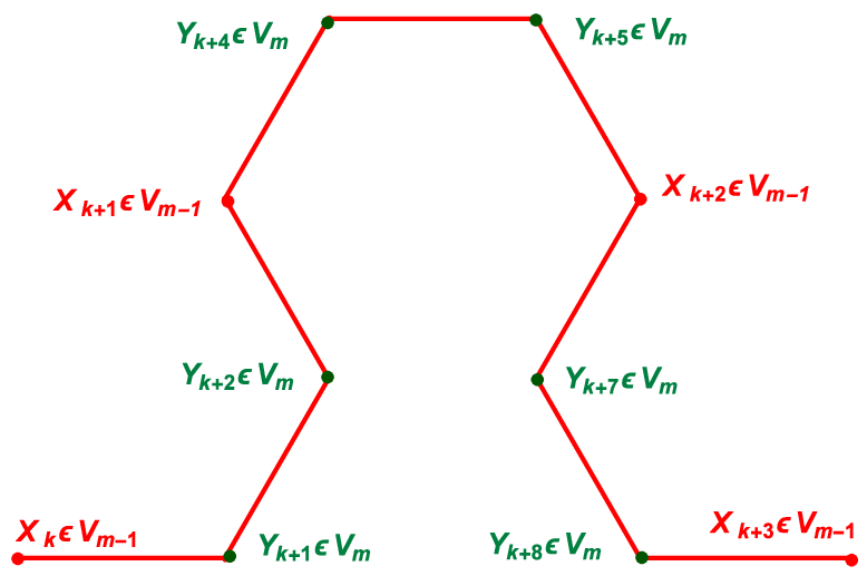
Y_{k}=X_{k}\quad,\quad Y_{k+3}=X_{k+1}\quad,\quad Y_{k+6}=X_{k+2}\quad,\quad Y_{k+9}=X_{k+3}

The eigenvalue equation in $\Lambda_{m}$ leads to the following system:

\left\{\begin{array}[]{ccccc}\left\{\Lambda_{m}-2\right\}\,u_{m}\left(Y_{k+i+1}\right)&=&-u_{m}\left(Y_{k+i}\right)-u_{m}\left(Y_{k+i+2}\right)&=&-u_{m-1}\left(X_{k+i}\right)-u_{m}\left(Y_{k+i+2}\right)\\ \left\{\Lambda_{m}-2\right\}\,u_{m}\left(Y_{k+i+2}\right)&=&-u_{m}\left(Y_{k+i+1}\right)-u_{m}\left(Y_{k+i+1}\right)&=&-u_{m-1}\left(X_{k+i+1}\right)-u_{m}\left(Y_{k+i+1}\right)\end{array}\right.\,,\,0\leqslant i\leqslant 2

The sequence $\left(u_{m}\left(Y_{k+i}\right)\right)_{0\leqslant i\leqslant 9}$ satisfies a second order recurrence relation, the characteristic equation of which is:

r^{2}+\left\{\Lambda_{m}-2\right\}\,r+1=0

The discriminant is:

\delta_{m}=\left\{\Lambda_{m}-2\right\}^{2}-4=\omega_{m}^{2}\quad,\quad\omega_{m}\,\in\,\mathbb{C}

The roots $r_{1,m}$ and $r_{2,m}$ of the characteristic equation are the scalar given by:

r_{1,m}=\displaystyle\frac{2-\Lambda_{m}-\omega_{m}}{2}\quad,\quad r_{2,m}=\displaystyle\frac{2-\Lambda_{m}+\omega_{m}}{2}

One has then, for any natural integer $i$ of $\left\{0,\ldots,9\right\}$ :

u_{m}\left(Y_{k+i}\right)=\alpha_{m}\,r_{1,m}^{i}+\beta_{m}\,r_{2,m}^{i}

where $\alpha_{m}$ and $\beta_{m}$ denote scalar constants.

The extension $u_{m}$ of $u_{m-1}$ to $V_{m}\setminus V_{1}$ has to be an eigenfunction of $\Delta_{m}$ , for the eigenvalue $\Lambda_{m}$ .
Since $u_{m-1}$ is an eigenfunction of $\Delta_{m-1}$ , for the eigenvalue $\Lambda_{m-1}$ , the sequence $\left(u_{m-1}\left(X_{k+i}\right)\right)_{0\leqslant i\leqslant 9}$ must itself satisfy a second order linear recurrence relation which be the pendant, at order $m$ , of the one satisfied by the sequence $\left(u_{m}\left(Y_{k+i}\right)\right)_{0\leqslant i\leqslant 9}$ , the characteristic equation of which is:

\left\{\Lambda_{m-1}-2\right\}\,r=-1-r^{2}

and discriminant:

\delta_{m-1}=\left\{\Lambda_{m-1}-2\right\}^{2}-4=\omega_{m-1}^{2}\quad,\quad\omega_{m-1}\,\in\,\mathbb{C}

The roots $r_{1,m-1}$ and $r_{2,m-1}$ of this characteristic equation are the scalar given by:

r_{1,m-1}=\displaystyle\frac{2-\Lambda_{m-1}-\omega_{m-1}}{2}\quad,\quad r_{2,m-1}=\displaystyle\frac{2-\Lambda_{m-1}+\omega_{m-1}}{2}

For any integer $i$ of $\left\{0,\ldots,9\right\}$ :

u_{m-1}\left(Y_{k+i}\right)=\alpha_{m-1}\,r_{1,m-1}^{i}+\beta_{m-1}\,r_{2,m-1}^{i}

where $\alpha_{m-1}$ and $\beta_{m-1}$ denote scalar constants.

From this point, the compatibility conditions, imposed by spectral decimation, have to be satisfied:

\left\{\begin{array}[]{ccc}u_{m}\left(Y_{k}\right)&=&u_{m-1}\left(X_{k}\right)\\ u_{m}\left(Y_{k+3}\right)&=&u_{m-1}\left(X_{k+1}\right)\\ u_{m}\left(Y_{k+6}\right)&=&u_{m-1}\left(X_{k+2}\right)\\ u_{m}\left(Y_{k+9}\right)&=&u_{m-1}\left(X_{k+3}\right)\\ \end{array}\right.

i.e.:

\left\{\begin{array}[]{ccccc}\alpha_{m}+\beta_{m}&=&\alpha_{m-1}+\beta_{m-1}&{\cal C}_{m}\\ \alpha_{m}\,r_{1,m}^{3}+\beta_{m}\,r_{2,m}^{3}&=&\alpha_{m-1}\,r_{1,m-1}+\beta_{m-1}\,r_{2,m-1}&{\cal C}_{1,m}\\ \alpha_{m}\,r_{1,m}^{6}+\beta_{m}\,r_{2,m}^{6}&=&\alpha_{m-1}\,r_{1,m-1}^{2}+\beta_{m-1}\,r_{2,m-1}^{2}&{\cal C}_{2,m}\\ \alpha_{m}\,r_{1,m}^{9}+\beta_{m}\,r_{2,m}^{9}&=&\alpha_{m-1}\,r_{1,m-1}^{3}+\beta_{m-1}\,r_{2,m-1}^{3}&{\cal C}_{3,m}\\ \end{array}\right.

where, for any natural integer $m$ , $\alpha_{m}$ and $\beta_{m}$ are scalar constants (real or complex).

Since the graph ${\cal SG}^{\cal C}_{m-1}$ is linked to the graph ${\cal SG}^{\cal C}_{m}$ by a similar process to the one that links ${\cal SG}^{\cal C}_{2}$ to ${\cal SG}^{\cal C}_{1}$ , one can legitimately consider that the constants $\alpha_{m}$ and $\beta_{m}$ do not depend on the integer $m$ :

\forall\,m\,\in\,{\mathbb{N}}^{\star}\,:\quad\alpha_{m}=\alpha\,\in\,{\mathbb{R}}\quad,\quad\beta_{m}=\beta\,\in\,{\mathbb{R}}

The above system writes:

\left\{\begin{array}[]{ccc}\alpha\,r_{1,m}^{3}+\beta\,r_{2,m}^{3}&=&\alpha\,r_{1,m-1}+\beta\,r_{2,m-1}\\ \alpha\,r_{1,m}^{6}+\beta\,r_{2,m}^{6}&=&\alpha\,r_{1,m-1}^{2}+\beta\,r_{2,m-1}^{2}\\ \alpha\,r_{1,m}^{8}+\beta\,r_{2,m}^{8}&=&\alpha\,r_{1,m-1}^{4}+\beta\,r_{2,m-1}^{4}\\ \end{array}\right.

One has then to consider the following configurations:

First case:

For any natural integer $m$ :

r_{1,m}\,\in\,{\mathbb{R}}\quad,\quad r_{2,m}\,\in\,{\mathbb{R}}

and, more precisely:

r_{1,m}<0\quad,\quad r_{2,m}<0

since the function $\varphi$ , which, to any real number $x\geqslant 4$ , associates:

\varphi(x)=\displaystyle\frac{2-x+\varepsilon\,\sqrt{\left\{x-2\right\}^{2}-4}}{2}\quad,\quad\varepsilon\,\in\,\left\{-1,1\right\}

is strictly increasing on $]4,+\infty[$ . Due to its continuity, is is a bijection of $]4,+\infty[$ on $\varphi\left(]4,+\infty[\right)=]-1,0[$ .

Let us introduce the function $\phi$ , which, to any real number $x\geqslant 2$ , associates:

\phi(x)=|\varphi(x)|=\displaystyle\frac{-2+x-\varepsilon\,\sqrt{\left\{x-2\right\}^{2}-4}}{2}

where $\varepsilon\,\in\,\left\{-1,1\right\}$ .

The function $\phi$ is a bijection of $]4,+\infty[$ on $\phi\left(]4,+\infty[\right)=]0,1[$ . We will denote by $\phi^{-1}$ its inverse bijection:

\forall\,\,x\,\in\,]0,1[\,:\quad\phi^{-1}(x)=\displaystyle\frac{(y+1)^{2}}{y}

One has then:

\varphi\left(\Lambda_{m-1}\right)=\displaystyle\frac{2-\Lambda_{m-1}+\varepsilon\,\omega_{m-1}}{2}\leqslant 0

This yields:

(-1)^{3}\,\left(\varphi\left(\Lambda_{m}\right)\right)^{3}=\varphi\left(\Lambda_{m-1}\right)\leqslant 0

which leads to:

\phi\left(\Lambda_{m}\right)=\left(\phi\left(\Lambda_{m-1}\right)\right)^{\frac{1}{3}}

and:

\Lambda_{m}=\phi^{-1}\left(\left(\phi\left(\Lambda_{m-1}\right)\right)^{\frac{1}{3}}\right)=\displaystyle\frac{\left\{\left(\phi\left(\Lambda_{m-1}\right)\right)^{\frac{1}{3}}+1\right\}^{2}}{\left(\phi\left(\Lambda_{m-1}\right)\right)^{\frac{1}{3}}}=\displaystyle\frac{\left\{\left(\displaystyle\frac{-2+\Lambda_{m-1}-\varepsilon\,\sqrt{\left\{\Lambda_{m-1}-2\right\}^{2}-4}}{2}\right)^{\frac{1}{3}}+1\right\}^{2}}{\left(\displaystyle\frac{-2+\Lambda_{m-1}-\varepsilon\,\sqrt{\left\{\Lambda_{m-1}-2\right\}^{2}-4}}{2}\right)^{\frac{1}{3}}}

ii.

Second case :

For any natural integer $m$ :

r_{1,m}\,\in\,\mathbb{C}\setminus{\mathbb{R}}\quad r_{2,m}=\overline{r_{1,m}}\,\in\,\mathbb{C}\setminus{\mathbb{R}}

Let us introduce:

\rho_{m}=\left|r_{1,m}\right|\,\in\,{\mathbb{R}}^{+}\quad,\quad\theta_{m}=\text{arg}\,r_{1,m}\quad\text{if}\quad r_{1,m}\neq 0

The above system writes:

\left\{\begin{array}[]{ccc}\rho_{m}^{3}\,\left\{\gamma\,\cos\left(3\,\theta_{m}\right)+\delta\,\sin\left(3\,\theta_{m}\right)\right\}&=&\rho_{m-1}\,\left\{\gamma\,\cos\left(\theta_{m-1}\right)+\delta\,\sin\left(\theta_{m-1}\right)\right\}\\ \rho_{m}^{6}\,\left\{\gamma\,\cos\left(6\,\theta_{m}\right)+\delta\,\sin\left(6\,\theta_{m}\right)\right\}&=&\rho_{m-1}^{2}\,\left\{\gamma\,\cos\left(2\,\theta_{m-1}\right)+\delta\,\sin\left(2\,\theta_{m-1}\right)\right\}\\ \rho_{m}^{9}\,\left\{\gamma\,\cos\left(9\,\theta_{m}\right)+\delta\,\sin\left(9\,\theta_{m}\right)\right\}&=&\rho_{m-1}^{3}\,\left\{\gamma\,\cos\left(3\,\theta_{m-1}\right)+\delta\,\sin\left(3\,\theta_{m-1}\right)\right\}\\ \end{array}\right.

where $\gamma$ and $\delta$ denote real constants.

The system is satisfied if:

\left\{\begin{array}[]{ccc}\rho_{m}^{3}&=&\rho_{m-1}\\ \theta_{m}&=&\displaystyle\frac{\theta_{m-1}}{3}\end{array}\right.

and thus:

\phi\left(\Lambda_{m}\right)=\left(\phi\left(\Lambda_{m-1}\right)\right)^{\frac{1}{N_{b}}}

which leads to the same relation as in the previous case:

\Lambda_{m}=\phi^{-1}\left(\left(\phi\left(\Lambda_{m-1}\right)\right)^{\frac{1}{3}}\right)=\displaystyle\frac{\left\{\left(\phi\left(\Lambda_{m-1}\right)\right)^{\frac{1}{3}}+1\right\}^{2}}{\left(\phi\left(\Lambda_{m-1}\right)\right)^{\frac{1}{3}}}=\displaystyle\frac{\left\{\left(\displaystyle\frac{-2+\Lambda_{m-1}-\varepsilon\,\sqrt{\left\{\Lambda_{m-1}-2\right\}^{2}-4}}{2}\right)^{\frac{1}{3}}+1\right\}^{2}}{\left(\displaystyle\frac{-2+\Lambda_{m-1}-\varepsilon\,\sqrt{\left\{\Lambda_{m-1}-2\right\}^{2}-4}}{2}\right)^{\frac{1}{3}}}

where $\varepsilon\,\in\,\left\{-1,1\right\}$ .

5 Detailed study of the spectrum of the Laplacian

As exposed by R. S. Strichartz in [20], one may bear in mind that the eigenvalues can be grouped into two categories:

i.

initial eigenvalues, which a priori belong to the set of forbidden values (as for instance $\Lambda=2$ ) ;
ii.

continued eigenvalues, obtained by means of spectral decimation.

We present, in the sequel, a detailed study of the spectrum of $\Delta$ .

5.1 Eigenvalues and eigenvectors of $\Delta_{2}$

Let us recall that the vertices of the graph ${\cal SG}^{\cal C}_{2}$ are:

X_{j}^{2}\quad,\quad 1\leqslant j\leqslant 10

with:

X_{1}^{2}=A\quad,\quad X_{4}^{2}=B\quad,\quad X_{7}^{2}=C\quad,\quad X_{10}^{2}=A

For the sake of simplicity, we will set here:

X_{2}^{2}=E\quad,\quad X_{3}^{2}=F\quad,\quad X_{5}^{2}=G\quad,\quad X_{6}^{2}=H\quad,\quad X_{8}^{2}=I\quad,\quad X_{9}^{2}=J

One may note that:

\text{Card}\,\left(V_{2}\setminus V_{1}\right)=10-4=6

Let us denote by $u$ an eigenfunction, for the eigenvalue $-\Lambda$ . Let us set:

u(A)=a\,\in\,{\mathbb{R}}\quad,\quad u(B)=b\,\in\,{\mathbb{R}}\quad,\quad u(C)=c\,\in\,{\mathbb{R}}\quad,\quad u(D)=d\,\in\,{\mathbb{R}}

u(E)=e\,\in\,{\mathbb{R}}\hskip 8.50012pt,\hskip 8.50012ptu(F)=f\,\in\,{\mathbb{R}}\hskip 8.50012pt,\hskip 8.50012ptu(G)=g\,\in\,{\mathbb{R}}\hskip 8.50012pt,\hskip 8.50012ptu(H)=h\,\in\,{\mathbb{R}}\hskip 8.50012pt,\hskip 8.50012ptu(I)=i\,\in\,{\mathbb{R}}\hskip 8.50012pt,\hskip 8.50012ptu(J)=j\,\in\,{\mathbb{R}}

One has then:

\left\{\begin{array}[]{ccc}a+f&=&-(\Lambda-2)\,e\\ b+e&=&-(\Lambda-2)\,f\\ b+h&=&-(\Lambda-2)\,g\\ g+c&=&-(\Lambda-2)\,h\\ c+j&=&-(\Lambda-2)\,i\\ i+d&=&-(\Lambda-2)\,j\\ \end{array}\right.

One may note that the only "Dirichlet eigenvalues", i.e. the ones related to the Dirichlet problem:

u_{|V_{1}}=0\quad\text{i.e.}\quad u(A)=u(B)=u(C)=u(D)=0

are obtained for:

\left\{\begin{array}[]{ccc}f&=&-(\Lambda-2)\,e\\ e&=&-(\Lambda-2)\,f\\ h&=&-(\Lambda-2)\,g\\ g&=&-(\Lambda-2)\,h\\ j&=&-(\Lambda-2)\,i\\ i&=&-(\Lambda-2)\,j\\ \end{array}\right.

i.e.:

\left\{\begin{array}[]{ccc}f&=&(\Lambda-2)^{2}\,f\\ e&=&(\Lambda-2)^{2}\,e\\ h&=&(\Lambda-2)\,h\\ g&=&(\Lambda-2)^{2}\,g\\ j&=&(\Lambda-2)^{2}\,i\\ i&=&(\Lambda-2)^{2}\,i\\ \end{array}\right.

The forbidden eigenvalue $\Lambda=2$ cannot thus be a Dirichlet one.

Let us consider the case where:

(\Lambda-2)^{2}=1

i.e.

\Lambda=1\quad\text{or}\quad\Lambda=3

which yields a three-dimensional eigenspace. The multiplicity of the eigenvalue $\Lambda=1$ is 3.

In the same way, the eigenvalue $\Lambda=3$ yields a three-dimensional eigenspace. the multiplicity of the eigenvalue $\Lambda=3$ is 3.

Since the cardinal of $V_{2}\setminus V_{1}$ is:

{\cal N}^{\cal S}_{2}-4=6

one may note that we have the complete spectrum.

5.2 Eigenvalues of $\Delta_{m}$ , $m\,\in\,{\mathbb{N}}$ , $m\geqslant 3$

As previously, one can easily check that the forbidden eigenvalue $\Lambda=2$ is not a Dirichlet one.

One can also check that $\Lambda_{m}=1$ and $\Lambda_{m}=3$ are eigenvalues of $\Delta_{m}$ .

By induction, one may note that, due to the spectral decimation, the initial eigenvalue $\Lambda_{2}=1$ gives birth, at this $m^{th}$ step, to eigenvalues $\Lambda_{\hookrightarrow 1,m}$ , and, in the same way, the initial eigenvalue $\Lambda_{2}=3$ gives birth, at this $m^{th}$ step, to eigenvalues $\Lambda_{\hookrightarrow 3,m}$ .
The dimension of the Dirichlet eigenspace is equal to the cardinal of $V_{m}\setminus V_{1}$ , i.e.:

{\cal N}^{\cal S}_{m}-{\cal N}^{\cal S}_{1}=3^{m}-3

\begin{array}[]{|c|c|c| }\hline\cr\\ \text{Level}&\text{Cardinal of the Dirichlet spectrum}\\ \hline\cr\\ m&3^{m}-3\\ \hline\cr\\ 2&6\\ \hline\cr\\ 3&24\\ \hline\cr\\ 4&78\\ \hline\cr\end{array}

Property 5.1.

Let us introduce:

\Lambda=\displaystyle\lim_{m\to+\infty}3^{-m}\,4^{m\,\delta}

One may note that, due to the definition of the Laplacian $\Delta$ , the limit exists.

5.3 Eigenvalue counting function

Definition 5.1.

Eigenvalue counting function

Let us introduce the eigenvalue counting function, related to ${\cal SG}^{\cal C}\setminus V_{1}$ , such that, for any positive number $x$ :

{\cal N}^{{\cal SG}^{\cal C}\setminus V_{1}}(x)=\text{Card}\,\left\{\Lambda\,\text{Dirichlet eigenvalue of~$-\Delta$}\,:\quad\Lambda\leqslant x\right\}

Property 5.2.

Given an integer $m\geqslant 2$ , the cardinal of $V_{m}\setminus V_{1}$ is:

{\cal N}^{\cal S}_{m}-{\cal N}^{\cal S}_{1}=3^{m}-3

This leads to the existence of a strictly positive constant $C$ such that:

{\cal N}^{{\cal SG}^{\cal C}}(C\,3^{-m}\,4^{m\,\delta})=3^{m}-3

If one looks for an asymptotic growth rate of the form

{\cal N}^{{\cal SG}^{\cal C}}(x)\sim x^{\alpha_{{\cal SG}^{\cal C}}}

one obtains:

\alpha_{{\cal SG}^{\cal C}}=\displaystyle\frac{\ln 3}{\delta\,\ln\frac{4}{3}}=\displaystyle\frac{\ln 3}{\frac{\ln 5}{\ln 4}\,\ln\frac{4}{3}}

which is not the same value as in the case of the Sierpiński gasket (we refer to [20]):

\alpha_{{\cal SG}}=\displaystyle\frac{\ln 3}{\ln 5}<\alpha_{{\cal SG}^{\cal C}}

It appears then that increasing the number of points, and the number of connections, decreases the value of the Weyl exponent $\alpha$ .

By following [20], one may note that the ratio

\displaystyle\frac{{\cal N}^{{\cal SG}^{\cal C}}(x)}{x}

is bounded above and away from zero, and admits a limit along any sequence of the form $C\,3^{-m}\,4^{m\,\delta}$ , $C>0$ ,
$m\geqslant 2$ . This enables one to deduce the existence of a periodic function $g$ , the period of which is equal to $\ln\displaystyle\frac{4^{\delta}}{3}$ , discontinuous at the value $\displaystyle\frac{4^{\delta}}{3}$ , such that:

\displaystyle\lim_{x\to+\infty}\left\{\displaystyle\frac{{\cal N}^{{\cal SG}^{\cal C}}(x)}{x}-g(\ln x)\right\}=0

References

[1] J. Kigami, A harmonic calculus on the Sierpiński spaces, Japan J. Appl. Math., 8 (1989), pages 259-290.
[2] J. Kigami, Harmonic calculus on p.c.f. self-similar sets, Trans. Amer. Math. Soc., 335(1993), pages 721-755.
[3] R. S. Strichartz, Densities of Self-Similar Measures on the Line, Experimental Mathematics, 4(2), 1995, pages 101-128.
[4] R. S. Strichartz, Analysis on fractals, Notices of the AMS, 46(8), 1999, pages 1199-1208.
[5] J. Kigami, R. S. Strichartz, K. C. Walker, Constructing a Laplacian on the Diamond Fractal, A. K. Peters, Ltd, Experimental Mathematics, 10(3), pages 437-448.
[6] Cl. David, Laplacian, on the graph of the Weierstrass function, arXiv:1703.03371v1.
[7] , U. Mosco, Energy Functionals on Certain Fractal Structures, Journal of Convex Analysis, 9(2), 2002, pages 581-600.
[8] U. R. Freiberg, M. R. Lancia, Energy Form on a Closed Fractal Curve, Journal for Analysis and its Applications, 23(1), 2004, pages 115-137.
[9] J. Kigami and M. Lapidus, Weyl’s problem for the spectral distribution of Laplacians on P.C.F. self-similar fractalss, Communications in Mathematical Physics, 204, 2003, pages 399-444.
[10] B. B. Mandelbrot, Fractals: form, chance, and dimension, San Francisco: Freeman, 1977.
[11] K. Falconer, The Geometry of Fractal Sets, 1985, Cambridge University Press, pages 114-149.
[12] M. F. Barnsley, S. Demko, Iterated Function Systems and the Global Construction of Fractals, The Proceedings of the Royal Society of London, A(399), 1985, pages 243-275.
[13] C. Sabot, Existence and uniqueness of diffusions on finitely ramified self-similar fractals, Annales scientifiques de l’É.N.S. 4 e série, 30(4), 1997, pages 605-673.
[14] A. Beurling, J. Deny, Espaces de Dirichlet. I. Le cas élémentaire, Acta Mathematica, 99 (1), 1985, pages 203-224.
[15] M. Fukushima, Y. Oshima, and M. Takeda, Dirichlet forms and symmetric Markov processes, 1994, Walter de Gruyter & Co.
[16] J. Kigami, Harmonic Analysis for Resistance Forms, Journal of Functional Analysis, 204, 2003, pages 399-444.
[17] N. Riane, 2016, Autour du Laplacien sur des domaines présentant un caractère fractal, Mémoire de recherche, M2 Mathématiques de la modélisation, Université Pierre et Marie Curie-Paris 6.
[18] Cl. David et N. Riane, Formes de Dirichlet et fonctions harmoniques sur le graphe de la fonction de Weierstrass, preprint, HAL.
[19] R. S. Strichartz, Function spaces on fractals, Journal of Functional Analysis, 198(1), 2003, pages 43-83.
[20] R. S. Strichartz, Differential Equations on Fractals, A tutorial, Princeton University Press, 2006.
[21] J. E. Hutchinson, Fractals and self similarity, Indiana University Mathematics Journal 30, 1981, pages 713-747.
[22] R. S. Strichartz, A. Taylor and T. Zhang, Densities of Self-Similar Measures on the Line, Experimental Mathematics, 4(2), 1995, pages 101-128.
[23] M. Fukushima and T. Shima, On a spectral analysis for the Sierpinski gasket, Potential Anal., 1, 1992, pages 1-3.

A note on energy forms on fractal domains

1 Introduction

2 Framework of the study

Notation.

Definition 2.1.

Property 2.1.

Property 2.2.

Definition 2.2.

Property 2.3.

Remark 2.1.

Notation.

Property 2.4.

Proof.

Property 2.5.

Definition 2.3.

Definition 2.4.

Definition 2.5.

Property 2.6.

Definition 2.6.

Notation.

Definition 2.7.

Property 2.7.

Property 2.8.

Definition 2.8.

Definition 2.9.

Definition 2.10.

Notation.

Definition 2.11.

Property 2.9.

Proposition 2.10.

Remark 2.2.

Definition 2.12.

Proposition 2.11.

Definition 2.13.

Definition 2.14.

Notation.

Notation.

3 Laplacian of a continuous function, on the Sierpiński arrowhead curve

Definition 3.1.

Property 3.1.

Definition 3.2.

Definition 3.3.

Definition 3.4.

Definition 3.5.

Definition 3.6.

Notation.

Property 3.2.

Property 3.3.

4 Explicit determination of the Laplacian of a function uu of dom​Δ\text{dom}\,\Delta

Theorem 4.1.

Proof.

4.1 Spectrum of the Laplacian

5 Detailed study of the spectrum of the Laplacian

5.1 Eigenvalues and eigenvectors of Δ2\Delta_{2}

5.2 Eigenvalues of Δm\Delta_{m}, m∈ℕm\,\in\,{\mathbb{N}}, m⩾3m\geqslant 3

Property 5.1.

5.3 Eigenvalue counting function

Definition 5.1.

Property 5.2.

References

4 Explicit determination of the Laplacian of a function $u$ of $\text{dom}\,\Delta$

5.1 Eigenvalues and eigenvectors of $\Delta_{2}$

5.2 Eigenvalues of $\Delta_{m}$ , $m\,\in\,{\mathbb{N}}$ , $m\geqslant 3$