Vessel Tracking via Sub-Riemannian Geodesics on $\mathbb{R}^{2}\times P^{1}$

In image analysis extraction of salient curves such as blood vessels, is often tackled by first lifting the image data to a new representation defined on the higher dimensional space of positions and directions, followed by a geodesic tracking [1, 2, 3] in this lifted space [4, 5, 6]. Benefits of such approaches are that one can generically deal with complex structures such as crossings [4, 6, 7], bifurcations [8], and low-contrast [5, 6, 9], while accounting for contextual alignment of local orientations [5, 6]. The latter can be done in the same way as in cortical models of visual perception of lines [10, 11, 12, 13], namely via sub-Riemannian (SR) geometry on the combined space of positions and orientations. In these cortical models, it is sometimes stressed [12] that one should work in a projective line bundle $\mathbb{R}^{2}\times P^{1}$ with a partition of equivalence classes $P^{1}:=S^{1}/_{\sim}$ with $\textbf{n}_{1}\sim\textbf{n}_{2}\Leftrightarrow\textbf{n}_{1}=\pm\textbf{n}_{2}$. Furthermore, in the statistics of line co-occurrences in retinal images the same projective line bundle structure is crucial [14]. Also, for many image analysis applications the orientation of an elongated structure is a well defined characteristic of a salient curve in an image, in contrast to an artificially imposed direction.

At first sight the effect of the identification of antipodal points might seem minor as the minimizing SR geodesic between two elements in $\mathbb{R}^{2}\times P^{1}$ is obtained by the minimum of the two minimizing SR geodesics in $\mathbb{R}^{2}\times S^{1}$ that arise (twice) by flipping the directions of the boundary conditions. However, this appearance is deceptive, it has a rather serious impact on geometric notions such as 1) the 1st Maxwell set (where two distinct geodesics with equal length meet for the first positive time), 2) the cut-locus (where a geodesic looses optimality), 3) the cusp-surface (where spatial projections of SR geodesics show a cusp). Besides an analysis of the geometric consequences in Sect. 2, 3, 4, we show that the projective line bundle provides a better tracking with much less cusps in Sect. 5.

At least for $\epsilon=0$ and $\mathcal{C}=1$ the assumption in Prop. 1 on conjugate points is obsolete by [18] and [7, Thm 3.2, App.D].

A sub-Riemannian sphere is a set of points equidistant from $e$. Thus, a sphere of radius $R$ centred at $e$ is given by $\mathcal{S}(R)=\left\{q\in\operatorname{PT}\nolimits(\mathbb{R}^{2})\,|\,\overline{d}(e,q)=R\right\}$. A Maxwell point is a point in $\operatorname{PT}\nolimits(\mathbb{R}^{2})$ connected to $e$ by multiple SR length minimizers. I.e. its multiplicity is $>1$. All Maxwell points form a Maxwell set:

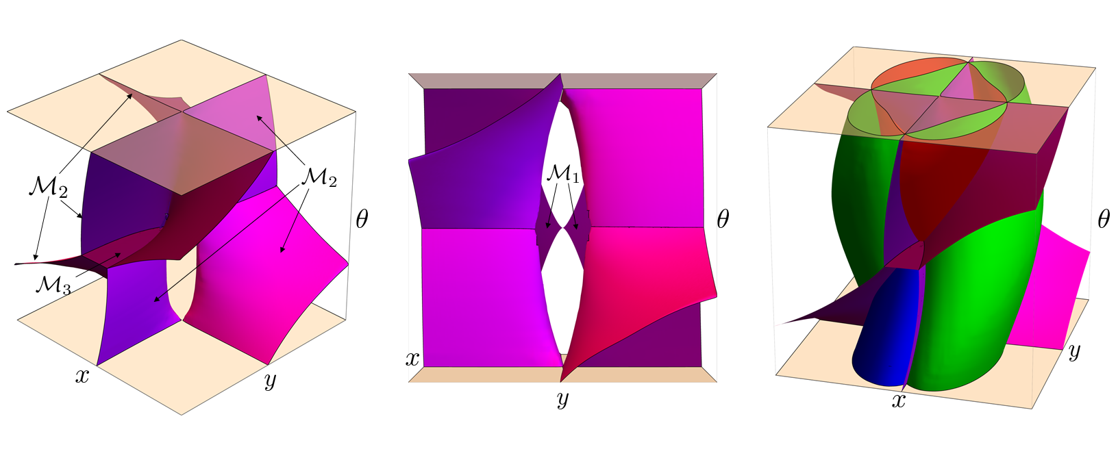
In SR geometry, an $n$-th Maxwell point is a point, where a geodesic meets another geodesic for the $n$-th time. In this work, by Maxwell point we mean the 1-st Maxwell point, where geodesics lose their optimality. The set $\mathcal{M}$ is a stratified manifold $\mathcal{M}=\bigcup_{i}\mathcal{M}_{i}$. We aim for maximal dimension strata: $\dim(\mathcal{M}_{i})=2$.

A cusp point $\textbf{x}(t_{0})$ on a spatial projection of a (SR) geodesic $t\mapsto(\textbf{x}(t),\theta(t))$ in $\mathbb{R}^{2}\times S^{1}$ is a point where the only spatial control switches sign, i.e. $u^{1}(t_{0}):=\dot{x}(t_{0})\cos\theta(t_{0})+\dot{y}(t_{0})\sin\theta(t_{0})\!=\!0\textrm{\, and }\ (u^{1})^{\prime}(t_{0})\neq 0$. In fact, the 2nd condition $(u^{1})^{\prime}(t_{0})\neq 0$ is obsolete [8, App.C]. The next proposition shows that the occurrence of cusps is greatly reduced in $\mathbb{R}^{2}\times P^{1}$.

Let $\gothic{R}\subset\mathbb{R}^{2}\times S^{1}$ denote the set of endpoints that can be connected to the origin $e=(0,0,0)$ by a SR geodesic $\gamma:[0,T]\to\mathbb{R}^{2}\times S^{1}$ whose spatial control $u^{1}(t)>0$ for all $t\in[0,T]$. Let $\tilde{\gothic{R}}\subset\mathbb{R}^{2}\times P^{1}$ denote the set of endpoints that can be connected to $e$ by a SR geodesic $\gamma:[0,T]\to\mathbb{R}^{2}\times S^{1}$ whose spatial control $u^{1}(t)$ does not switch sign for all $t\in[0,T]$. Henceforth, such a SR geodesic whose spatial control $u^{1}(\cdot)$ does not switch sign will be called ‘cuspless’ geodesic.

Set $\gothic{R}$ yields a single cone field of reachable angles in $x>0$, see​ [21, fig 14,​ thm​ 9]. By Prop.​ 4, set $\tilde{\gothic{R}}$ is a union of 2 such cone fields that is also reflected to $x<0$.

Distance $W(q)$ can be numerically obtained by solving the eikonal PDE of Eq. (6) via similar approaches as was previously done for the $\operatorname{SE(2)}\nolimits$ case. E.g., via an iterative upwind scheme [7], or a fast marching solver [22] in which case the SR metric tensor is approximated by an anisotropic Riemannian metric tensor [23]. A gradient descent (cf. Eq. (5)) on $W$ then provides the SR geodesics.

We construct the cost function $\mathcal{C}$ in the same way as in [7]: (1) a retinal image is lifted via the orientation score transform using cake wavelets [24]; (2) vessels are enhanced via left-invariant Gaussian derivatives using $\mathcal{A}_{3}$; (3) a cost function is constructed via $\mathcal{C}=\frac{1}{1+\lambda\mathcal{V}^{p}}$, with $\mathcal{V}$ the max-normalized vessel enhanced orientation score, and with $\lambda$ and $p$ respectively a “cost-strength” and contrast parameter. We use the same data and settings ($\lambda=100$, $p=3$ and $\xi=0.01$) as in [7], and perform vessel tracking on 235 vessel segments. For the results on all retinal image patches, see http://erikbekkers.bitbucket.io/PTR2.html.

Fig. 4 shows the results on three different vessel segments with comparison between SR geodesics in $\operatorname{SE(2)}\nolimits$ and $\operatorname{PT}\nolimits(\mathbb{R}^{2})$. As expected, with the $\operatorname{PT}\nolimits(\mathbb{R}^{2})$ model we always obtain the $\operatorname{SE(2)}\nolimits$ geodesic with minimum SR length (cf. Eq. (4)). This has the advantage that overall we encounter less cusps in the tracking. Additionally, the $\operatorname{PT}\nolimits(\mathbb{R}^{2})$ model is approximately four times faster since now we only have to consider half of the domain $\mathbb{R}^{2}\times S^{1}$, and by (6) we only need to run once (instead of twice). The average computation time for constructing $W$ with the $\operatorname{SE(2)}\nolimits$ model for $180\times 140$ pixel patches is $14.4$ seconds, whereas for the $\operatorname{PT}\nolimits(\mathbb{R}^{2})$ model this is only 3.4 seconds. The rightmost image in Fig. 4 shows an exceptional case in which the reversed boundary condition (red arrow) is preferred as this leads to a geodesic with only one cusp instead of two. Recent work [8] proposes to deal with such cusp problems by relying on a positive control model ($u_{1}>0$), introducing more natural corner points instead of cusps. Also there one benefits from working with the projective line bundle [8, Fig.12].

We have shown the effect of including the projective line bundle structure SR in optimal geodesic tracking (Prop.​ 1), in SR geometry (Prop.​ 2), and in Maxwell-stratification (Prop.​ 3), and in the occurrence of cusps in spatially projected geodesics (Prop.​ 4). It supports our experiments that show benefits of including such a projective line bundle structure: A better vessel tracking algorithm with a reduction of cusps and computation time. As the cusp-free model without reverse gear [8] also benefits [8, Fig.12] from $\operatorname{PT}\nolimits(\mathbb{R}^{2})$-structure, we leave the Maxwell stratification of this combined model for future work.

References

• [1] G. Peyré, M. Péchaud, R. Keriven, L.D. Cohen, Geodesic methods in computer vision and graphics, Foundations and Trends in Computer Graphics and Vision, 5(3–4), 197–397, 2010.
• [2] V. Caselles, R. Kimmel, G. Sapiro, Geodesic Active Contours, IJCV, 22(1), 61–79, 1997.
• [3] L. Cohen, R. Kimmel, Global minimum for active contour models, IJCV, 24(1), 57–78, 1997.
• [4] M. Péchaud, R. Keriven, G. Peyré, Extraction of tubular structures over an orientation domain, In IEEE conf. on CVPR, 336–342, 2009.
• [5] E.J. Bekkers, Retinal Image Analysis using Sub-Riemannian Geometry in SE(2), PhD thesis, Eindhoven University of Technology, Biomedical Engineering, 2017.
• [6] D. Chen, New Minimal Path Models for Tubular Structure Extraction and Image Segmentation, PhD thesis, Universit´e Paris Dauphine, PSL Research Univ., 2016.
• [7] E.J. Bekkers, R. Duits, A. Mashtakov, G. Sanguinetti, A PDE approach to data-driven sub-riemannian geodesics in SE(2), SIAM-SIIMS, 8(4), 2740–2770, 2015.
• [8] R. Duits, S. Meesters, J. Mirebeau, J. Portegies, Optimal paths for variants of the 2d and 3d Reeds-Shepp car with applications in image analysis, (arXiv:1612.06137), 2017.
• [9] J. Zhang, B. Dashtbozorg, E. Bekkers, J. Pluim, R. Duits, B. ter Haar Romeny, Robust retinal vessel segmentation via locally adaptive derivative frames in orientation scores, IEEE TMI, 35 (12), 2631–2644, 2016.
• [10] G. Citti, A. Sarti, A cortical based model of perceptual completion in the roto-translation space, JMIV, 24(3), 307–326, 2006.
• [11] J. Petitot, Vers une Neuro-gèométrie. Fibrations corticales, structures de contact et contours subjectifs modaux, Math. Inf. Sci. Humaines, 145, 5–-101, 1999.
• [12] U. Boscain, R. Duits, F. Rossi, Y. Sachkov, Curve cuspless reconstruction via sub-Riemannian geometry, ESAIM:COCV, 20, 748–770, 2014.
• [13] A.P. Mashtakov, A.A. Ardentov, Y.L. Sachkov, Parallel algorithm and software for image inpainting via sub-Riemannian minimizers on the group of rototranslations, NMTMA, 6(1), 95–115, 2013.
• [14] S. Abbasi-Sureshjani, J. Zhang, R. Duits, B. ter Haar Romeny, Retrieving challenging vessel connections in retinal images by line co-occurence statistics, preprint: (arXiv:1610.06368), to appear in Biological Cybernetics 2017.
• [15] A.A. Agrachev, Yu.L. Sachkov, Control Theory from the Geometric Viewpoint, Springer-Verlag, 2004.
• [16] A. Bressan, Viscosity Solutions of Hamilton-Jacobi Equations and Optimal Control Problems, Lecture Notes Dep. of Math., Pennsylvania State University, 2011.
• [17] A.A. Agrachev, D. Barilari, U. Boscain, Introduction to Riemannian and Sub-Riemannian Geometry from the Hamiltonian Viewpoint, preprint SISSA 09/2012/M november 20, 2016.
• [18] Y.L. Sachkov, Conjugate and cut time in the sub-Riemannian problem on the group of motions of a plane, ESAIM:COCV, 16(4), 1018–1039, 2009.
• [19] I. Moiseev, Y. L. Sachkov, Maxwell strata in sub-Riemannian problem on the group of motions of a plane, ESAIM:COCV, 16(2), 380–399, 2010.
• [20] Yu.L. Sachkov, Cut locus and optimal synthesis in the sub-Riemannian problem on the group of motions of a plane, ESAIM:COCV, 17(2), 293–321, 2011.
• [21] R. Duits, U. Boscain, F. Rossi, Y. Sachkov, Association fields via cuspless sub-Riemannian geodesics in SE(2), JMIV, 49(2), 384–417, 2014.
• [22] J.-M. Mirebeau, Anisotropic Fast-Marching on cartesian grids using Lattice Basis Reduction, SIAM J. Num. Anal., 52(4), 1573–1599, 2014.
• [23] G. Sanguinetti, E.J. Bekkers, R. Duits, M.H.J. Janssen, A. Mashtakov, J.-M. Mirebeau, Sub-Riemannian fast marching in SE(2), LNCS, 366–374, 2015.
• [24] R. Duits, M. Felsberg, G. Granlund, B.M. ter Haar Romeny, Image analysis and reconstruction using a wavelet transform constructed from a reducible representation of the Euclidean motion group, IJCV, 72(1), 79–102, 2007.