跳到论文正文
W Papers独立论文阅读器 arXiv:1704.03575 论文正文 计算阅读时间 · 0%
引用这篇论文根据当前论文元数据生成,正式投稿前建议核对。


License: arXiv.org perpetual non-exclusive license
arXiv:1704.03575v3 [math-ph] 21 Jun 2017

Izergin-Korepin analysis on the projected wavefunctions of the generalized free-fermion model

Kohei Motegi ††thanks: E-mail: kmoteg0@kaiyodai.ac.jp Affiliation: Faculty of Marine Technology, Tokyo University of Marine Science and Technology, Affiliation: Etchujima 2-1-6, Koto-Ku, Tokyo, 135-8533, Japan
August 24, 2026
Abstract

We apply the Izergin-Korepin analysis to the study of the projected wavefunctions of the generalized free-fermion model. We introduce a generalization of the LL-operator of the six-vertex model by Bump-Brubaker-Friedberg and Bump-McNamara-Nakasuji. We make the Izergin-Korepin analysis to characterize the projected wavefunctions and show that they can be expressed as a product of factors and certain symmetric functions which generalizes the factorial Schur functions. This result can be seen as a generalization of the Tokuyama formula for the factorial Schur functions.

1 Introduction

Integrable lattice models [1, 2, 3, 4] are special classes of models in statistical physics which many exact calculations are believed to be able to be done. The most local object in integrable models is called as the RR-matrix, and its mathematical structure was revealed in the mid 1980s [5, 6]. The underlying mathematical structure was named as the quantum groups, and the investigation of the quantum groups naturally lead to immediate constructions of various RR-matrices.

From the point of view of statistical physics, RR-matrices are the most local objects, and the study on the RR-matrices is a starting point. The most important objects in statistical physics are partition functions. For the case of integrable models, partition functions are objects constructed from multiple RR-matrices and are determined by boundary conditions. One of the most famous partition functions in integrable lattice models are the domain wall boundary partition functions which was first introduced and analyzed in [7, 8]. In recent years, a more general class of partition functions which we shall call as the projected wavefunctions are attracting attention in its relation with algebraic combinatorics. The projected wavefunctions are the projection of the off-shell Bethe vector of integrable models into a class of some simple states labelled by the sequences of the particles or down spins. For the case of the free-fermion model in an external field, it was first shown by Bump-Brubaker-Friedberg [9] that the projected wavefunctions give a natural realization of the Tokuyama combinatorial formula for the Schur functions [10], which is a one-parameter deformation of the Weyl character formula (note there are pioneering works using the free-fermion model implicitly in [11, 12, 13], and the Izergin-Korepin analysis and observation of the factorization phenomena on the domain wall boundary partition functions of the related models called as the Perk-Schultz (supersymmetric vertex) model [14] and the Felderhof free-fermion model [15] in [16, 17]. There is also an application to the correlation functions in [18]). This observation triggered studies on finding various generalizations and variations of the Tokuyama-type formula for symmetric functions [19, 20, 21, 22, 23, 24, 25, 26, 27] such as the factorial Schur functions and symplectic Schur functions, and an interesting notion was introduced furthermore which the number theorists call as the metaplectic ice.

In this paper, we analyze the free-fermion model using the method initiated by Izergin-Korepin [7, 8]. The method was developed by them in order to find the explicit expression of polynomials representing the domain wall boundary partition functions of the Uq​(s​l2)U_{q}(sl_{2}) six-vertex model, from which the famous Izergin-Korepin determinant formula was found. The Izergin-Korepin analysis is the important method to study variants of the domain wall boundary partition functions. For example, it was applied to the domain wall boundary partition functions of the Uq​(s​l2)U_{q}(sl_{2}) six-vertex model with reflecting end by Tsuchiya [28] to find its determinant formula. Extending the Izergin-Korepin analysis to more general class of partition functions are also important. Wheeler [29] invented a method to extend the Izergin-Korepin analysis on a class of partition functions called the scalar products. And in our very recent work [30], we extended the Izergin-Korepin analysis to study the projected wavefunctions of the Uq​(s​l2)U_{q}(sl_{2}) six-vertex model. The resulting symmetric polynomials representing the projected wavefunctions contains the Grothendieck polynomials as a special case when the six-vertex model reduces to the five-vertex model [31, 32, 33]. We apply this technique to study the free-fermion model in an external field. To this end, we first introduce an ultimate generalization of the LL-operator by introducing the inhomogeneous parameters and factorial parameters. We use an inhomogeneous version of the generalized LL-operator in our forthcoming paper [34] having two types of factorial parameters, which generalizes the factorial LL-operator by Bump-McNamara-Nakasuji [22]. We next view the projected wavefunctions as a function of the inhomogeneous parameters and characterize its properties by using the Izergin-Korepin analysis. We then show that the product of factors and certain symmetric functions satisfies all the required properties the projected wavefunctions must satisfy. The result is a generalization of the [9] and [22], hence can be viewed as a generalization of the Tokuyama for the factorial Schur functions. The Izergin-Korepin analysis views the partition functions as functions of inhomogeneous parameters in the quantum spaces, whereas the arguments initiated in [9] view the partition functions as functions of the free parameter in the auxiliary spaces. The comparison of the two different ways of arguments seems to be interesting.

We will use the results of the projected wavefunctions to the algebraic combinatorial study of the generalized Schur functions [34]. For example, two ways of evaluations of the same partition functions can lead to integrable model constructions of algebraic identities of the symmetric functions. For example, two ways of evaluations of the domain wall boundary partition functions, a direct evaluation and an indirect evaluation using the completeness relation and the projected wavefunctions, can give rise to the dual Cauchy formula of the generalized Schur functions. This idea can also be applied to partition functions of integrable models under reflecting boundary to give dual Cauchy identities of the generalized symplectic Schur functions. Further detailed Izergin-Korepin analysis on the domain wall boundary partition functions and the dual projected wavefunctions are required for the studies.

There are also studies on deriving Cauchy identities using the domain wall boundary partition functions like an intertwiner, invented in [35]. Deriving algebraic combinatorial properties of symmetric functions using their integrable model realizations is an active line of research. See [36, 37, 38, 39, 40] for more examples on Cauchy-type identities and more recent studies on the Littlewood-Richardson coefficients by [33, 41].

In any case, in order to do these studies, we first of all have to find out what are the explicit functions representing the projected wavefunctions. We think the Izergin-Korepin analysis presented in this paper is a fairly simple way to find out the explicit forms.

This paper is organized as follows. In the next section, we first list the generalized LL-operator and introduce the projected wavefunctions. In section 3, we make the Izergin-Korepin analysis and list the properties needed to determine the explicit form of the projected wavefunctions. In section 4, we show that the product of factors and certain symmetric functions satisfies all the required properties extracted from the Izergin-Korepin analysis, which means that the product is the explicit form of the projected wavefunctions. Section 5 is devoted to the conclusion of this paper.

2 The generalized free-fermion model and the projected wavefunctions

The most fundamental objects in integrable lattice models are the RR-matrices and LL-operators. The RR-matrix of the free-fermion model we treat in this paper is given by

Ra​b​(z)=(1+t​z0000t⁡(1−z)t+100(t+1)​zz−10000z+t),\displaystyle R_{ab}(z)=\left(\begin{array}[]{cccc}1+tz&0&0&0\\ 0&t(1-z)&t+1&0\\ 0&(t+1)z&z-1&0\\ 0&0&0&z+t\end{array}\right),

acting on the tensor product Wa⊗WbW_{a}\otimes W_{b} of the complex two-dimensional space WaW_{a}.

Refer to caption
Figure 1: The LL-operator La​j​(z,wj,αj,γj)L_{aj}(z,w_{j},\alpha_{j},\gamma_{j}) (2). The horizontal line is the space WaW_{a}, and the vertical line is the space ℱj\mathcal{F}_{j}.

The LL-operator of the free-fermion model we use as bulk pieces of the projected wavefunctions in this paper is given by

La​j​(z,wj,αj,γj)\displaystyle L_{aj}(z,w_{j},\alpha_{j},\gamma_{j})
=\displaystyle= (wj−γj​z0000t​wj+γj​zwj00(t+1)​zαj​wj+(1−αj​γj)​z0000−t​αj​wj+(1−αj​γj)​z),\displaystyle\left(\begin{array}[]{cccc}w_{j}-\gamma_{j}z&0&0&0\\ 0&tw_{j}+\gamma_{j}z&w_{j}&0\\ 0&(t+1)z&\alpha_{j}w_{j}+(1-\alpha_{j}\gamma_{j})z&0\\ 0&0&0&-t\alpha_{j}w_{j}+(1-\alpha_{j}\gamma_{j})z\end{array}\right),

acting on the tensor product Wa⊗ℱjW_{a}\otimes\mathcal{F}_{j} of the space WaW_{a} and the two-dimensional Fock space at the jjth site ℱj\mathcal{F}_{j}.

The parameters wjw_{j}, αj\alpha_{j} and γj\gamma_{j} can be regarded as parameters associated with the quantum space ℱj\mathcal{F}_{j}. The LL-operators giving the Schur functions [9] and factorial Schur functions [22] is a special limit of the generalized LL-operator (2) given by

La​j​(z,1,0,0)=(10000t100(t+1)​zz0000z),\displaystyle L_{aj}(z,1,0,0)=\left(\begin{array}[]{cccc}1&0&0&0\\ 0&t&1&0\\ 0&(t+1)z&z&0\\ 0&0&0&z\end{array}\right),
La​j​(z,1,αj,0)=(10000t100(t+1)​zαj+z0000−t​αj+z),\displaystyle L_{aj}(z,1,\alpha_{j},0)=\left(\begin{array}[]{cccc}1&0&0&0\\ 0&t&1&0\\ 0&(t+1)z&\alpha_{j}+z&0\\ 0&0&0&-t\alpha_{j}+z\end{array}\right),

respectively.

The LL-operator (2) together with the RR-matrix (2) satisfies the R​L​LRLL relation

Ra​b​(z1/z2)​La​j​(z1,wj,αj,γj)​Lb​j​(z2,wj,αj,γj)\displaystyle R_{ab}(z_{1}/z_{2})L_{aj}(z_{1},w_{j},\alpha_{j},\gamma_{j})L_{bj}(z_{2},w_{j},\alpha_{j},\gamma_{j})
=\displaystyle= Lb​j​(z2,wj,αj,γj)​La​j​(z1,wj,αj,γj)​Ra​b​(z1/z2),\displaystyle L_{bj}(z_{2},w_{j},\alpha_{j},\gamma_{j})L_{aj}(z_{1},w_{j},\alpha_{j},\gamma_{j})R_{ab}(z_{1}/z_{2}), (2.20)

acting on Wa⊗Wb⊗ℱjW_{a}\otimes W_{b}\otimes\mathcal{F}_{j}.

Let us denote the orthonormal basis of WaW_{a} and its dual as {|0⟩a,|1⟩a}\{|0\rangle_{a},|1\rangle_{a}\} and {⟨0|,⟨1|}aa\{{}_{a}\langle 0|,{}_{a}\langle 1|\}, and the orthonormal basis of ℱj\mathcal{F}_{j} and its dual as {|0⟩j,|1⟩j}\{|0\rangle_{j},|1\rangle_{j}\} and {⟨0|,⟨1|}jj\{{}_{j}\langle 0|,{}_{j}\langle 1|\}. The matrix elements of the LL-operator can be written as ⟨γ|⟨δ|La​j(z,wj,αj,γj)|α⟩aj|β⟩ja{}_{a}\langle\gamma|{}_{j}\langle\delta|L_{aj}(z,w_{j},\alpha_{j},\gamma_{j})|\alpha\rangle_{a}|\beta\rangle_{j}, which we will use this form in the next section. See Figure 1 for a pictorial description of the LL-operator (2).

The RR-matrices and the LL-operators have origins in statistical physics, and |0⟩|0\rangle or its dual ⟨0|\langle 0| can be regarded as a hole state, while |1⟩|1\rangle or its dual ⟨1|\langle 1| can be interpretted as a particle state from the point of view of statistical physics. We sometimes use the terms hole states and particle states to describe states constructed from |0⟩|0\rangle, ⟨0|\langle 0|, |1⟩|1\rangle and ⟨1|\langle 1| since they are convenient for the description of the states. In the quantum inverse scattering method, the Fock spaces WaW_{a} and ℱj\mathcal{F}_{j} are usually called the auxiliary and quantum spaces, respectively.

For later convenience, we also define the following Pauli spin operators σ+\sigma^{+} and σ−\sigma^{-} as operators acting on the (dual) orthonomal basis as

σ+​|1⟩=|0⟩,σ+​|0⟩=0,⟨0|​σ+=⟨1|,⟨1|​σ+=0,\displaystyle\sigma^{+}|1\rangle=|0\rangle,\ \sigma^{+}|0\rangle=0,\ \langle 0|\sigma^{+}=\langle 1|,\ \langle 1|\sigma^{+}=0, (2.21)
σ−​|0⟩=|1⟩,σ−​|1⟩=0,⟨1|​σ−=⟨0|,⟨0|​σ−=0.\displaystyle\sigma^{-}|0\rangle=|1\rangle,\ \sigma^{-}|1\rangle=0,\ \langle 1|\sigma^{-}=\langle 0|,\ \langle 0|\sigma^{-}=0. (2.22)
Refer to caption
Figure 2: The monodromy matrix Ta​(z|w1,…,wM)T_{a}(z|w_{1},\dots,w_{M}) (2.23) (top) and the BB-operator B⁡(z|w1,…,wM)B(z|w_{1},\dots,w_{M}) (bottom).
Refer to caption
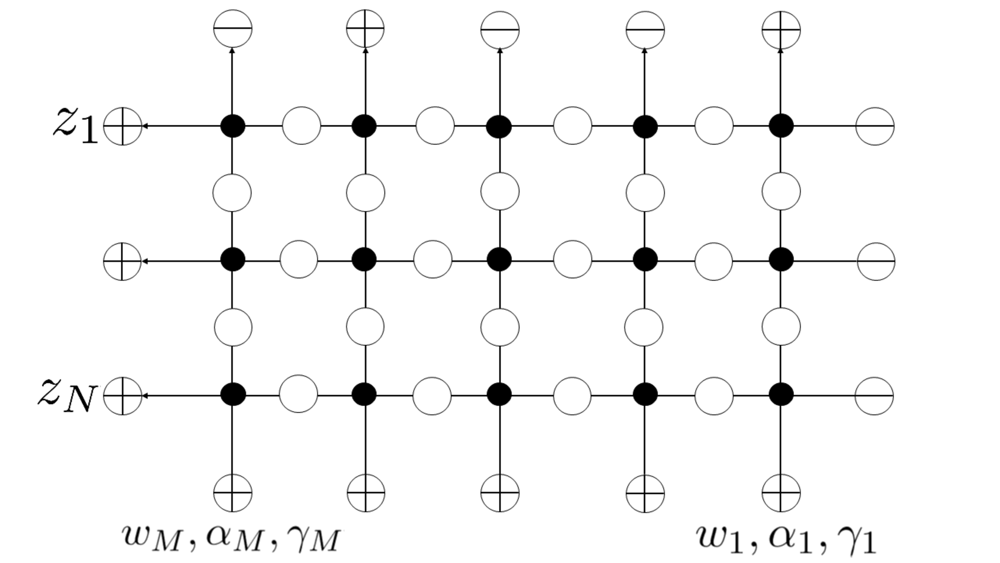
Figure 3: The projected wavefunctions WM,N(z1,…,zN|w1,…,wM|x1,…,xN)W_{M,N}(z_{1},\dots,z_{N}|w_{1},\dots,w_{M}|x_{1},\dots,x_{N}) (2.26). This figure illustrates the case M=5M=5, N=3N=3, x1=2x_{1}=2, x2=3x_{2}=3, x3=5x_{3}=5.

To construct projected wavefunctions, we introduce the monodromy matrix Ta​(z|w1,…,wM)T_{a}(z|w_{1},\dots,w_{M}) (Figure 2 top) from the generalized LL-operator (2) as

Ta​(z|w1,…,wM)\displaystyle T_{a}(z|w_{1},\dots,w_{M}) =La​M(z,wM,αM,γM)⋯La​1(z,w1,α1,γ1)\displaystyle=L_{aM}(z,w_{M},\alpha_{M},\gamma_{M})\cdots L_{a1}(z,w_{1},\alpha_{1},\gamma_{1})
=(A⁡(z|w1,…,wM)B⁡(z|w1,…,wM)C⁡(z|w1,…,wM)D⁡(z|w1,…,wM))a∈End(Wa⊗ℱ1⊗⋯⊗ℱM).\displaystyle=\begin{pmatrix}A(z|w_{1},\dots,w_{M})&B(z|w_{1},\dots,w_{M})\\ C(z|w_{1},\dots,w_{M})&D(z|w_{1},\dots,w_{M})\end{pmatrix}_{a}\in\mathrm{End}(W_{a}\otimes\mathcal{F}_{1}\otimes\cdots\otimes\mathcal{F}_{M}). (2.23)

The matrix elements A⁡(z|w1,…,wM),B⁡(z|w1,…,wM),C⁡(z|w1,…,wM)A(z|w_{1},\dots,w_{M}),B(z|w_{1},\dots,w_{M}),C(z|w_{1},\dots,w_{M})
and D⁡(z|w1,…,wM)D(z|w_{1},\dots,w_{M}) are called as the A​B​C​DABCD operators, which are 2M×2M2^{M}\times 2^{M} matrices acting on the tensor product of the quantum spaces ℱ1⊗⋯⊗ℱM\mathcal{F}_{1}\otimes\dots\otimes\mathcal{F}_{M}.

To create projected wavefunctions, what is important is the BB-operator B⁡(z|w1,…,wM)B(z|w_{1},\dots,w_{M}) (Figure 2 bottom) which has the role of creating particles in the quantum spaces ℱ1⊗⋯⊗ℱM\mathcal{F}_{1}\otimes\cdots\otimes\mathcal{F}_{M}. We next introduce the following state vector
|ΦM,N(z1,…,zN|w1,…,wM)⟩∈ℱ1⊗⋯⊗ℱM|\Phi_{M,N}(z_{1},\dots,z_{N}|w_{1},\dots,w_{M})\rangle\in\mathcal{F}_{1}\otimes\cdots\otimes\mathcal{F}_{M} using the BB-operators as

|ΦM,N(z1,…,zN|w1,…,wM)⟩=B(z1|w1,…,wM)⋯B(zN|w1,…,wM)|Ω⟩M,\displaystyle|\Phi_{M,N}(z_{1},\dots,z_{N}|w_{1},\dots,w_{M})\rangle=B(z_{1}|w_{1},\dots,w_{M})\cdots B(z_{N}|w_{1},\dots,w_{M})|\Omega\rangle_{M}, (2.24)

where |Ω⟩M:=|0⟩1⊗⋯⊗|0⟩M∈ℱ1⊗⋯⊗ℱM|\Omega\rangle_{M}:=|0\rangle_{1}\otimes\cdots\otimes|0\rangle_{M}\in\mathcal{F}_{1}\otimes\cdots\otimes\mathcal{F}_{M} is the vacuum state in the tensor product of quantum spaces.

Due to the so-called ice rule of the LL-operator ⟨γ|⟨δ|La​j(z,wj,αj,γj)|α⟩aj|β⟩ja=0{}_{a}\langle\gamma|{}_{j}\langle\delta|L_{aj}(z,w_{j},\alpha_{j},\gamma_{j})|\alpha\rangle_{a}|\beta\rangle_{j}=0 unless α+β=γ+δ\alpha+\beta=\gamma+\delta, each BB-operator creates one particle in the quantum spaces. This fact and that the state vector (2.24) is constructed from NN-layers of the BB-operators acting on the vacuum state |Ω⟩M|\Omega\rangle_{M}, the state vector (2.24) is an NN-particle state for N≤MN\leq M. To construct a nonvanishing inner product, we introduce the dual NN-particle state

⟨x1⋯xN|\displaystyle\langle x_{1}\cdots x_{N}| =(1⟨0|⊗⋯⊗⟨0|)M∏j=1Nσxj+∈ℱ1∗⊗⋯⊗ℱM∗,\displaystyle=(_{1}\langle 0|\otimes\cdots\otimes{}_{M}\langle 0|)\prod_{j=1}^{N}\sigma^{+}_{x_{j}}\in\mathcal{F}_{1}^{*}\otimes\cdots\otimes\mathcal{F}_{M}^{*}, (2.25)

which are states labelling the configurations of particles 1≤x1<x2<⋯<xN≤M1\leq x_{1}<x_{2}<\cdots<x_{N}\leq M.

The projected wavefunctions WM,N(z1,…,zN|w1,…,wM|x1,…,xN)W_{M,N}(z_{1},\dots,z_{N}|w_{1},\dots,w_{M}|x_{1},\dots,x_{N}) is defined as the inner product between the state vector (off-shell Bethe vector) |ΦM,N(z1,…,zN|w1,…,wM)⟩|\Phi_{M,N}(z_{1},\dots,z_{N}|w_{1},\dots,w_{M})\rangle and the NN-particle state ⟨x1⋯xN|\langle x_{1}\cdots x_{N}|

WM,N(z1,…,zN|w1,…,wM|x1,…,xN)=⟨x1⋯xN|ΦM,N(z1,…,zN|w1,…,wM)⟩.\displaystyle W_{M,N}(z_{1},\dots,z_{N}|w_{1},\dots,w_{M}|x_{1},\dots,x_{N})=\langle x_{1}\cdots x_{N}|\Phi_{M,N}(z_{1},\dots,z_{N}|w_{1},\dots,w_{M})\rangle. (2.26)

See Figure 3 for a pictorial description of (2.26).

In the next section, we examine the properties of the projected wavefunctions. Here we just remark that the projected wavefunctions of the free-fermion model treated in this paper is not symmetric with respect to the spectral parameters {z1,…,zN}\{z_{1},\dots,z_{N}\}. This is in contrast to the case of the projected wavefunctions of the Uq​(s​l2)U_{q}(sl_{2}) six-vertex model, where they are symmetric with respect to the spectral variables, in which case the Grothendieck polynomials and its quantum group deformation appears. This fact for the properties of the spectral variables of the free-fermion model lead to the Tokuyama formula [10] for the Schur functions, as was first found in [9].

3 Izergin-Korepin analysis

By the Izergin-Korepin analysis, we examine the properties of the projected wavefunctions
WM,N(z1,…,zN|w1,…,wM|x1,…,xN)W_{M,N}(z_{1},\dots,z_{N}|w_{1},\dots,w_{M}|x_{1},\dots,x_{N}) in this section.

Proposition 3.1.

The projected wavefunctions WM,N(z1,…,zN|w1,…,wM|x1,…,xN)W_{M,N}(z_{1},\dots,z_{N}|w_{1},\dots,w_{M}|x_{1},\dots,x_{N}) satisfies the following properties.

(1) WM,N(z1,…,zN|w1,…,wM|x1,…,xN)W_{M,N}(z_{1},\dots,z_{N}|w_{1},\dots,w_{M}|x_{1},\dots,x_{N}) is a polynomial of degree NN in wMw_{M}.
(2) The projected wavefunctions WM,N(zσ⁡(1),…,zσ⁡(N)|w1,…,wM|x1,…,xN)W_{M,N}(z_{\sigma(1)},\dots,z_{\sigma(N)}|w_{1},\dots,w_{M}|x_{1},\dots,x_{N}) with the ordering of the spectral parameters permuted zσ⁡(1),…,zσ⁡(N)z_{\sigma(1)},\dots,z_{\sigma(N)}, σ∈SN\sigma\in S_{N} are related with the unpermuted one WM,N(z1,…,zN|w1,…,wM|x1,…,xN)W_{M,N}(z_{1},\dots,z_{N}|w_{1},\dots,w_{M}|x_{1},\dots,x_{N}) by the following relation

∏1≤j<k≤Nσ⁡(j)>σ⁡(k)(zσ⁡(j)+tzσ⁡(k))WM,N(z1,…,zN|w1,…,wM|x1,…,xN)\displaystyle\prod_{\begin{subarray}{c}1\leq j<k\leq N\\ \sigma(j)>\sigma(k)\end{subarray}}(z_{\sigma(j)}+tz_{\sigma(k)})W_{M,N}(z_{1},\dots,z_{N}|w_{1},\dots,w_{M}|x_{1},\dots,x_{N})
=\displaystyle= ∏1≤j<k≤Nσ⁡(j)>σ⁡(k)(zσ⁡(k)+tzσ⁡(j))WM,N(zσ⁡(1),…,zσ⁡(N)|w1,…,wM|x1,…,xN).\displaystyle\prod_{\begin{subarray}{c}1\leq j<k\leq N\\ \sigma(j)>\sigma(k)\end{subarray}}(z_{\sigma(k)}+tz_{\sigma(j)})W_{M,N}(z_{\sigma(1)},\dots,z_{\sigma(N)}|w_{1},\dots,w_{M}|x_{1},\dots,x_{N}). (3.1)

(3) The following recursive relations between the projected wavefunctions hold if xN=Mx_{N}=M:

WM,N(z1,…,zN|w1,…,wM|x1,…,xN)|wM=γM​zN\displaystyle W_{M,N}(z_{1},\dots,z_{N}|w_{1},\dots,w_{M}|x_{1},\dots,x_{N})|_{w_{M}=\gamma_{M}z_{N}}
=\displaystyle= γMN​zN​∏j=1N−1(zj+t​zN)​∏j=1M−1{(1−αj​γj)​zN+αj​wj}\displaystyle\gamma_{M}^{N}z_{N}\prod_{j=1}^{N-1}(z_{j}+tz_{N})\prod_{j=1}^{M-1}\{(1-\alpha_{j}\gamma_{j})z_{N}+\alpha_{j}w_{j}\}
×WM−1,N−1(z1,…,zN−1|w1,…,wM−1|x1,…,xN−1).\displaystyle\times W_{M-1,N-1}(z_{1},\dots,z_{N-1}|w_{1},\dots,w_{M-1}|x_{1},\dots,x_{N-1}). (3.2)

When evaluated at wM=0w_{M}=0, we have

WM,N(z1,…,zN|w1,…,wM|x1,…,xN)|wM=0=0.\displaystyle W_{M,N}(z_{1},\dots,z_{N}|w_{1},\dots,w_{M}|x_{1},\dots,x_{N})|_{w_{M}=0}=0. (3.3)

If xN≠Mx_{N}\neq M, the following factorizations hold for the projected wavefunctions:

WM,N(z1,…,zN|w1,…,wM|x1,…,xN)\displaystyle W_{M,N}(z_{1},\dots,z_{N}|w_{1},\dots,w_{M}|x_{1},\dots,x_{N})
=\displaystyle= ∏j=1N(wM−γMzj)WM−1,N(z1,…,zN|w1,…,wM−1|x1,…,xN).\displaystyle\prod_{j=1}^{N}(w_{M}-\gamma_{M}z_{j})W_{M-1,N}(z_{1},\dots,z_{N}|w_{1},\dots,w_{M-1}|x_{1},\dots,x_{N}). (3.4)

(4) The following holds for the case N=1N=1, xN=Mx_{N}=M

WM,1(z|w1,…,wM|M)=wM∏k=1M−1{(1−αkγk)z+αkwk}.\displaystyle W_{M,1}(z|w_{1},\dots,w_{M}|M)=w_{M}\prod_{k=1}^{M-1}\{(1-\alpha_{k}\gamma_{k})z+\alpha_{k}w_{k}\}. (3.5)
Proof.

Let us first show Properties (1) and (3) for the case xN=Mx_{N}=M.

To show Property (1) when xN=Mx_{N}=M, we first express the projected wavefunctions in terms of the vertical transfer matrix

𝒯jN​(wj,z1,…,zN)=\displaystyle\mathcal{T}_{j}^{N}(w_{j};z_{1},\dots,z_{N})= La1​j(z1,wj,αj,γj)⋯LaN​j(zN,wj,αj,γj)\displaystyle L_{a_{1}j}(z_{1},w_{j},\alpha_{j},\gamma_{j})\cdots L_{a_{N}j}(z_{N},w_{j},\alpha_{j},\gamma_{j})
∈End(Wa1⊗⋯⊗WaN⊗ℱj).\displaystyle\in\mathrm{End}(W_{a_{1}}\otimes\cdots\otimes W_{a_{N}}\otimes\mathcal{F}_{j}). (3.6)

Using this vertical transfer matrix, the projected wavefunctions can be rewritten as

WM,N(z1,…,zN|w1,…,wM|x1,…,xN−1,M)\displaystyle W_{M,N}(z_{1},\dots,z_{N}|w_{1},\dots,w_{M}|x_{1},\dots,x_{N-1},M)
=\displaystyle= ⟨0|⊗N⟨1|⟨x1⋯xN−1|𝒯MN(wM;z1,…,zN)⋯𝒯1N(w1;z1,…,zN)|1⟩⊗N|Ω⟩MM,\displaystyle\langle 0|^{\otimes N}{}_{M}\langle 1|\langle x_{1}\cdots x_{N-1}|\mathcal{T}_{M}^{N}(w_{M};z_{1},\dots,z_{N})\cdots\mathcal{T}_{1}^{N}(w_{1};z_{1},\dots,z_{N})|1\rangle^{\otimes N}|\Omega\rangle_{M}, (3.7)
⟨0|⊗N=⟨0|⊗⋯⊗⟨0|,aNa1\displaystyle\langle 0|^{\otimes N}={}_{a_{1}}\langle 0|\otimes\cdots\otimes{}_{a_{N}}\langle 0|, (3.8)
|1⟩⊗N=|1⟩a1⊗⋯⊗|1⟩aN.\displaystyle|1\rangle^{\otimes N}=|1\rangle_{a_{1}}\otimes\cdots\otimes|1\rangle_{a_{N}}. (3.9)

Inserting the completeness relation in one particle sector

∑j=1N|0j−1,1,0N−j⟩⟨0j−1,1,0N−j|=Id,\displaystyle\sum_{j=1}^{N}|0^{j-1},1,0^{N-j}\rangle\langle 0^{j-1},1,0^{N-j}|=\mathrm{Id}, (3.10)
|0j−1,1,0N−j⟩=|0⟩a1⊗⋯⊗|0⟩aj−1⊗|1⟩aj⊗|0⟩aj+1⊗⋯⊗|0⟩aN,\displaystyle|0^{j-1},1,0^{N-j}\rangle=|0\rangle_{a_{1}}\otimes\cdots\otimes|0\rangle_{a_{j-1}}\otimes|1\rangle_{a_{j}}\otimes|0\rangle_{a_{j+1}}\otimes\cdots\otimes|0\rangle_{a_{N}}, (3.11)
⟨0j−1,1,0N−j|=⟨0|⊗⋯⊗⟨0|⊗⟨1|⊗⟨0|⊗⋯⊗⟨0|,aNaj+1ajaj−1a1\displaystyle\langle 0^{j-1},1,0^{N-j}|={}_{a_{1}}\langle 0|\otimes\cdots\otimes{}_{a_{j-1}}\langle 0|\otimes{}_{a_{j}}\langle 1|\otimes{}_{a_{j+1}}\langle 0|\otimes\cdots\otimes{}_{a_{N}}\langle 0|, (3.12)

into (3.9), we have

WM,N(z1,…,zN|w1,…,wM|x1,…,xN−1,M)\displaystyle W_{M,N}(z_{1},\dots,z_{N}|w_{1},\dots,w_{M}|x_{1},\dots,x_{N-1},M)
=\displaystyle= ∑j=1N⟨0|⊗N⟨1|𝒯MN(wM;z1,⋯,zN)|0j−1,1,0N−j⟩M|0⟩M\displaystyle\sum_{j=1}^{N}\langle 0|^{\otimes N}{}_{M}\langle 1|\mathcal{T}_{M}^{N}(w_{M};z_{1},\cdots,z_{N})|0^{j-1},1,0^{N-j}\rangle|0\rangle_{M}
×⟨x1⋯xN−1|⟨0j−1,1,0N−j|𝒯M−1N(wM−1;z1,⋯,zN)⋯𝒯1N(w1;z1,⋯,zN)|Ω⟩M−1|1⟩⊗N.\displaystyle\times\langle x_{1}\cdots x_{N-1}|\langle 0^{j-1},1,0^{N-j}|\mathcal{T}_{M-1}^{N}(w_{M-1};z_{1},\cdots,z_{N})\cdots\mathcal{T}_{1}^{N}(w_{1};z_{1},\cdots,z_{N})|\Omega\rangle_{M-1}|1\rangle^{\otimes N}. (3.13)

In the right hand side of (3.13), the parameter wMw_{M} depends only on
⟨0|⊗N⟨1|𝒯MN(wM;z1,⋯,zN)|0j−1,1,0N−j⟩M|0⟩M\langle 0|^{\otimes N}{}_{M}\langle 1|\mathcal{T}_{M}^{N}(w_{M};z_{1},\cdots,z_{N})|0^{j-1},1,0^{N-j}\rangle|0\rangle_{M}, whose matrix elements can be easily calculated from its graphical representation as

⟨0|⊗N⟨1|𝒯MN(wM;z1,⋯,zN)|0j−1,1,0N−j⟩M|0⟩M=wM∏k=1j−1(twM+γMzk)∏k=j+1N(wM−γMzk).\displaystyle\langle 0|^{\otimes N}{}_{M}\langle 1|\mathcal{T}_{M}^{N}(w_{M};z_{1},\cdots,z_{N})|0^{j-1},1,0^{N-j}\rangle|0\rangle_{M}=w_{M}\prod_{k=1}^{j-1}(tw_{M}+\gamma_{M}z_{k})\prod_{k=j+1}^{N}(w_{M}-\gamma_{M}z_{k}). (3.14)

Since the matrix elements (3.14) is a polynomial of degree NN in wMw_{M}, one finds that the projected wavefunctions is a polynomial of degree NN in wMw_{M}.

Let us next show Property (3) for the case xN=Mx_{N}=M. We first remark that since the projected wavefunctions WM,N(z1,…,zN|w1,…,wM|x1,…,xN)W_{M,N}(z_{1},\dots,z_{N}|w_{1},\dots,w_{M}|x_{1},\dots,x_{N}) is a polynomial of degree NN in wMw_{M}, one needs to evaluate N+1N+1 distinct points in wMw_{M} for the Izergin-Korepin trick to be successful. (3.2) is the result of the evaluation at the point wM=γM​zNw_{M}=\gamma_{M}z_{N}. The (N−1)(N-1) points wM=γM​zjw_{M}=\gamma_{M}z_{j}, j=1,…,N−1j=1,\dots,N-1 can be evaluated using Property (2), hence if one shows that certain functions satisfy Property (2), it remains to consider the evaluation at wM=γM​zNw_{M}=\gamma_{M}z_{N}. The evaluation at wM=γM​zNw_{M}=\gamma_{M}z_{N} essentially gives evaluations at NN distinct points. We need one more point to be evaluated. An easy point to be evaluated is wM=0w_{M}=0, whose result is (3.3). Let us show these two results of the evaluations.

The recursion relation (3.2) can be shown as follows. First, from the decomposition (3.13) and the explicit form of the matrix elements (3.14), one finds that after the substitution wM=γM​zNw_{M}=\gamma_{M}z_{N}, only the term j=Nj=N of the sum in (3.13) survives and we have

WM,N(z1,…,zN|w1,…,wM|x1,…,xN−1,M)|wM=γM​zN\displaystyle W_{M,N}(z_{1},\dots,z_{N}|w_{1},\dots,w_{M}|x_{1},\dots,x_{N-1},M)|_{w_{M}=\gamma_{M}z_{N}}
=\displaystyle= γMN​zN​∏j=1N−1(zj+t​zN)\displaystyle\gamma_{M}^{N}z_{N}\prod_{j=1}^{N-1}(z_{j}+tz_{N})
×⟨x1⋯xN−1|⟨0N−1,1|𝒯M−1N(wM−1;z1,⋯,zN)⋯𝒯1N(w1;z1,⋯,zN)|Ω⟩M−1|1⟩⊗N.\displaystyle\times\langle x_{1}\cdots x_{N-1}|\langle 0^{N-1},1|\mathcal{T}_{M-1}^{N}(w_{M-1};z_{1},\cdots,z_{N})\cdots\mathcal{T}_{1}^{N}(w_{1};z_{1},\cdots,z_{N})|\Omega\rangle_{M-1}|1\rangle^{\otimes N}. (3.15)

Since we can calculate the right hand side of (3.15) furthermore as

⟨x1⋯xN−1|⟨0N−1,1|𝒯M−1N(wM−1;z1,⋯,zN)⋯𝒯1N(w1;z1,⋯,zN)|Ω⟩M−1|1⟩⊗N\displaystyle\langle x_{1}\cdots x_{N-1}|\langle 0^{N-1},1|\mathcal{T}_{M-1}^{N}(w_{M-1};z_{1},\cdots,z_{N})\cdots\mathcal{T}_{1}^{N}(w_{1};z_{1},\cdots,z_{N})|\Omega\rangle_{M-1}|1\rangle^{\otimes N}
=\displaystyle= ⟨x1⋯xN−1|⟨0N−1|𝒯M−1N−1(wM−1;z1,⋯,zN−1)⋯𝒯1N−1(w1;z1,⋯,zN−1)|Ω⟩M−1|1⟩⊗N−1\displaystyle\langle x_{1}\cdots x_{N-1}|\langle 0^{N-1}|\mathcal{T}_{M-1}^{N-1}(w_{M-1};z_{1},\cdots,z_{N-1})\cdots\mathcal{T}_{1}^{N-1}(w_{1};z_{1},\cdots,z_{N-1})|\Omega\rangle_{M-1}|1\rangle^{\otimes N-1}
×⟨1|⟨Ω|LaN,M−1(zN,wM−1,αM−1,γM−1)⋯LaN,1(zN,w1,α1,γ1)|1⟩aNM−1|Ω⟩M−1aN\displaystyle\times{}_{a_{N}}\langle 1|{}_{M-1}\langle\Omega|L_{a_{N},M-1}(z_{N},w_{M-1},\alpha_{M-1},\gamma_{M-1})\cdots L_{a_{N},1}(z_{N},w_{1},\alpha_{1},\gamma_{1})|1\rangle_{a_{N}}|\Omega\rangle_{M-1}
=\displaystyle= WM−1,N−1(z1,…,zN−1|w1,…,wM−1|x1,…,xN−1)∏j=1M−1{(1−αjγj)zN+αjwj},\displaystyle W_{M-1,N-1}(z_{1},\dots,z_{N-1}|w_{1},\dots,w_{M-1}|x_{1},\dots,x_{N-1})\prod_{j=1}^{M-1}\{(1-\alpha_{j}\gamma_{j})z_{N}+\alpha_{j}w_{j}\}, (3.16)

we can express the evaluation of WM,N(z1,…,zN|w1,…,wM|x1,…,xN)W_{M,N}(z_{1},\dots,z_{N}|w_{1},\dots,w_{M}|x_{1},\dots,x_{N}) at wM=γM​zNw_{M}=\gamma_{M}z_{N} as

WM,N(z1,…,zN|w1,…,wM|x1,…,xN)|wM=γM​zN\displaystyle W_{M,N}(z_{1},\dots,z_{N}|w_{1},\dots,w_{M}|x_{1},\dots,x_{N})|_{w_{M}=\gamma_{M}z_{N}}
=\displaystyle= γMN​zN​∏j=1N−1(zj+t​zN)​∏j=1M−1{(1−αj​γj)​zN+αj​wj}\displaystyle\gamma_{M}^{N}z_{N}\prod_{j=1}^{N-1}(z_{j}+tz_{N})\prod_{j=1}^{M-1}\{(1-\alpha_{j}\gamma_{j})z_{N}+\alpha_{j}w_{j}\}
×WM−1,N−1(z1,…,zN−1|w1,…,wM−1|x1,…,xN−1).\displaystyle\times W_{M-1,N-1}(z_{1},\dots,z_{N-1}|w_{1},\dots,w_{M-1}|x_{1},\dots,x_{N-1}). (3.17)

The evaluation at wM=0w_{M}=0 (3.3) can be easily seen by the expansion (3.13) and the fact that all the matrix elements (3.14) contain the factor wMw_{M}.

Properties (1) and (3) for the case xN≠Mx_{N}\neq M can be shown much easier. Using the ice rule ⟨γ|⟨δ|La​j(z,wj,αj,γj)|α⟩aj|β⟩ja=0{}_{a}\langle\gamma|{}_{j}\langle\delta|L_{aj}(z,w_{j},\alpha_{j},\gamma_{j})|\alpha\rangle_{a}|\beta\rangle_{j}=0, one can easily finds the following factorization

WM,N(z1,…,zN|w1,…,wM|x1,…,xN)\displaystyle W_{M,N}(z_{1},\dots,z_{N}|w_{1},\dots,w_{M}|x_{1},\dots,x_{N})
=\displaystyle= ⟨0|⊗N⟨0|⟨x1⋯xN|𝒯MN(wM;z1,…,zN)⋯𝒯1N(w1;z1,…,zN)|1⟩⊗N|Ω⟩MM\displaystyle\langle 0|^{\otimes N}{}_{M}\langle 0|\langle x_{1}\cdots x_{N}|\mathcal{T}_{M}^{N}(w_{M};z_{1},\dots,z_{N})\cdots\mathcal{T}_{1}^{N}(w_{1};z_{1},\dots,z_{N})|1\rangle^{\otimes N}|\Omega\rangle_{M}
=\displaystyle= ⟨0|⊗N⟨0|𝒯MN(wM;z1,…,zN)|0⟩⊗NM|0⟩M\displaystyle\langle 0|^{\otimes N}{}_{M}\langle 0|\mathcal{T}_{M}^{N}(w_{M};z_{1},\dots,z_{N})|0\rangle^{\otimes N}|0\rangle_{M}
×⟨0|⊗N⟨x1⋯xN|𝒯M−1N(wM−1;z1,…,zN)⋯𝒯1N(w1;z1,…,zN)|1⟩⊗N|Ω⟩M−1\displaystyle\times\langle 0|^{\otimes N}\langle x_{1}\cdots x_{N}|\mathcal{T}_{M-1}^{N}(w_{M-1};z_{1},\dots,z_{N})\cdots\mathcal{T}_{1}^{N}(w_{1};z_{1},\dots,z_{N})|1\rangle^{\otimes N}|\Omega\rangle_{M-1}
=\displaystyle= ∏j=1N⟨0|⟨0|Laj,M(zj,wM,αM,γM)|0⟩ajM|0⟩Maj\displaystyle\prod_{j=1}^{N}{}_{a_{j}}\langle 0|{}_{M}\langle 0|L_{a_{j},M}(z_{j},w_{M},\alpha_{M},\gamma_{M})|0\rangle_{a_{j}}|0\rangle_{M}
×WM−1,N(z1,…,zN|w1,…,wM−1|x1,…,xN)\displaystyle\times W_{M-1,N}(z_{1},\dots,z_{N}|w_{1},\dots,w_{M-1}|x_{1},\dots,x_{N})
=\displaystyle= ∏j=1N(wM−γMzj)WM−1,N(z1,…,zN|w1,…,wM−1|x1,…,xN).\displaystyle\prod_{j=1}^{N}(w_{M}-\gamma_{M}z_{j})W_{M-1,N}(z_{1},\dots,z_{N}|w_{1},\dots,w_{M-1}|x_{1},\dots,x_{N}). (3.18)

This shows Properties (1) and (3) for the case xN≠Mx_{N}\neq M.

Property (2) can be shown as follows. Using the R​L​LRLL relation repeatedly, one gets the intertwining relation between the monodromy matrices

Ra​b​(z1/z2)​Ta​(z1|w1,…,wM)​Tb​(z2|w1,…,wM)\displaystyle R_{ab}(z_{1}/z_{2})T_{a}(z_{1}|w_{1},\dots,w_{M})T_{b}(z_{2}|w_{1},\dots,w_{M})
=\displaystyle= Tb​(z2|w1,…,wM)​Ta​(z1|w1,…,wM)​Ra​b​(z1/z2).\displaystyle T_{b}(z_{2}|w_{1},\dots,w_{M})T_{a}(z_{1}|w_{1},\dots,w_{M})R_{ab}(z_{1}/z_{2}). (3.19)

An element of the intertwining relation (3.19) gives the commutation relation between the BB-operators

(z2+t​z1)​B​(z1|w1,…,wM)​B​(z2|w1,…,wM)\displaystyle(z_{2}+tz_{1})B(z_{1}|w_{1},\dots,w_{M})B(z_{2}|w_{1},\dots,w_{M})
=\displaystyle= B⁡(z2|w1,…,wM)​B​(z1|w1,…,wM)​(z1+t​z2).\displaystyle B(z_{2}|w_{1},\dots,w_{M})B(z_{1}|w_{1},\dots,w_{M})(z_{1}+tz_{2}). (3.20)

Since the projected wavefunctions WM,N(z1,…,zN|w1,…,wM|x1,…,xN)W_{M,N}(z_{1},\dots,z_{N}|w_{1},\dots,w_{M}|x_{1},\dots,x_{N}) (2.26) are constructed from NN-layers of BB-operators, the effect of reordering the spectral parameters of the BB-operators can be traced using the commutation relation (3.20).

What finally remains is Property (4), which can also easily calculated. ∎

Before presenting the solution in the next section, we explain here why the Izergin-Korepin analysis uniquely defines the projected wavefunctions. The idea is based on the following fact: if there are two polynomials f⁡(w)f(w) and g⁡(w)g(w) of ww of degree NN, and the evaluations of the two polynomials at N+1N+1 distinct points are the same (f⁡(w)=g⁡(w)f(w)=g(w) for w=zjw=z_{j}, j=1,…,N+1j=1,\dots,N+1 such that zj≠zkz_{j}\neq z_{k}, j≠kj\neq k), then the two polynomials are exactly the same, i.e., f⁡(w)=g⁡(w)f(w)=g(w) for all ww. The idea of Izergin-Korepin analysis is to relate the projected wavefunctions WM,N(z1,…,zN|w1,…,wM|x1,…,xN)W_{M,N}(z_{1},\dots,z_{N}|w_{1},\dots,w_{M}|x_{1},\dots,x_{N}) with smaller ones by using the above fact. The point is to regard WM,N(z1,…,zN|w1,…,wM|x1,…,xN)W_{M,N}(z_{1},\dots,z_{N}|w_{1},\dots,w_{M}|x_{1},\dots,x_{N}) as a polynomial of a single variable wMw_{M}. By Property (1) in Proposition 3.1, WM,N(z1,…,zN|w1,…,wM|x1,…,xN)W_{M,N}(z_{1},\dots,z_{N}|w_{1},\dots,w_{M}|x_{1},\dots,x_{N}) is a polynomial of degree NN in wMw_{M}. If xN=Mx_{N}=M, one can evaluate the projected wavefunction at the following N+1N+1 points wM=γM​zjw_{M}=\gamma_{M}z_{j}, j=1,…,Nj=1,\dots,N, wM=0w_{M}=0. The evaluations at wM=γM​zNw_{M}=\gamma_{M}z_{N} and wM=0w_{M}=0 can be obtained by its graphical representation and can be expressed by using the smaller projected wavefuntion WM−1,N−1(z1,…,zN−1|w1,…,wM−1|x1,…,xN−1)W_{M-1,N-1}(z_{1},\dots,z_{N-1}|w_{1},\dots,w_{M-1}|x_{1},\dots,x_{N-1}), which is (3.2) and (3.3) of Property (3). The evaluations at (N−1)(N-1) points wM=γM​zjw_{M}=\gamma_{M}z_{j}, j=1,…,N−1j=1,\dots,N-1 can be obtained from the evaluation at wM=γM​zNw_{M}=\gamma_{M}z_{N} using Property (2). This idea is essentially the same with the Izergin-Korepin analysis for the domain wall boundary partition functions.

For the case of projected wavefunctions, there is another case we have to consider: the case when xN≠Mx_{N}\neq M. For this case, it is easier to connect the projected wavefunctions from its graphical description, and we have (3.4). Note that the smaller projected wavefunctions connected is
WM−1,N(z1,…,zN|w1,…,wM−1|x1,…,xN)W_{M-1,N}(z_{1},\dots,z_{N}|w_{1},\dots,w_{M-1}|x_{1},\dots,x_{N}) which is different from the one for the case when xN=Mx_{N}=M.

In both cases xN=Mx_{N}=M and xN≠Mx_{N}\neq M, we are able to connect the projected wavefunctions of different sizes, and continuing this process successively, the relations can be regarded as recursion relations between projected wavefunctions. For the Izergin-Korepin analysis to be successful such that it gives the uniqueness of the projected wavefunctions, we need the intitial condition for the recursion relations, and it is Property (4) in Proposition 3.1. Hence, if one finds an explicit function satisfying all the properties in Proposition 3.1, it is the one representing the projected wavefunctions. This is given in the next section.

4 Generalized Schur functions

Definition 4.1.

We define the following symmetric function
FM,N(z1,…,zN|w1,…,wM|x1,…,xN)F_{M,N}(z_{1},\dots,z_{N}|w_{1},\dots,w_{M}|x_{1},\dots,x_{N}) which depends on the symmetric variables z1,…,zNz_{1},\dots,z_{N}, complex parameters w1,…,wMw_{1},\dots,w_{M}, α1,…,αM\alpha_{1},\dots,\alpha_{M}, γ1,…,γM\gamma_{1},\dots,\gamma_{M} and integers x1,…,xNx_{1},\dots,x_{N} satisfying 1≤x1<⋯<xN≤M1\leq x_{1}<\cdots<x_{N}\leq M,

FM,N(z1,…,zN|w1,…,wM|x1,…,xN)\displaystyle F_{M,N}(z_{1},\dots,z_{N}|w_{1},\dots,w_{M}|x_{1},\dots,x_{N})
=\displaystyle= ∏j=1Nwxj​1∏1≤j<k≤N(zk−zj)​∑σ∈SN(−1)σ​∏j=1N∏k=xj+1M(wk−γk​zσ⁡(j))\displaystyle\prod_{j=1}^{N}w_{x_{j}}\frac{1}{\prod_{1\leq j<k\leq N}(z_{k}-z_{j})}\sum_{\sigma\in S_{N}}(-1)^{\sigma}\prod_{j=1}^{N}\prod_{k=x_{j}+1}^{M}(w_{k}-\gamma_{k}z_{\sigma(j)})
×∏j=1N∏k=1xj−1{(1−αk​γk)​zσ⁡(j)+αk​wk}.\displaystyle\times\prod_{j=1}^{N}\prod_{k=1}^{x_{j}-1}\{(1-\alpha_{k}\gamma_{k})z_{\sigma(j)}+\alpha_{k}w_{k}\}. (4.1)

The symmetric function FM,N(z1,…,zN|w1,…,wM|x1,…,xN)F_{M,N}(z_{1},\dots,z_{N}|w_{1},\dots,w_{M}|x_{1},\dots,x_{N}) (4.1) is a generalization of the (factorial) Schur functions. (4.1) can be rewritten in the form using Young diagrams as

FM,N(z1,…,zN|w1,…,wM|x1,…,xN)=Fλ+δ​(𝐳|w1,…,wM)∏1≤j<k≤N(zj−zk).\displaystyle F_{M,N}(z_{1},\dots,z_{N}|w_{1},\dots,w_{M}|x_{1},\dots,x_{N})=\frac{F_{\lambda+\delta}({\bf z}|w_{1},\dots,w_{M})}{\prod_{1\leq j<k\leq N}(z_{j}-z_{k})}. (4.2)

Here, 𝐳={z1,…,zN}{\bf z}=\{z_{1},\dots,z_{N}\} is a set of variables and λ\lambda denotes a Young diagram λ=(λ1,λ2,…,λN)\lambda=(\lambda_{1},\lambda_{2},\dots,\lambda_{N}) with weakly decreasing non-negative integers λ1≥λ2≥⋯≥λN≥0\lambda_{1}\geq\lambda_{2}\geq\cdots\geq\lambda_{N}\geq 0, and δ=(N−1,N−2,…,0)\delta=(N-1,N-2,\dots,0). Fμ​(𝐳​|{α}|​{γ})F_{\mu}({\bf z}|\{\alpha\}|\{\gamma\}) is an N×NN\times N determinant

Fμ​(𝐳|w1,…,wM)=detN​(fμj​(zk|w1,…,wM)),\displaystyle F_{\mu}({\bf z}|w_{1},\dots,w_{M})=\mathrm{det}_{N}(f_{\mu_{j}}(z_{k}|w_{1},\dots,w_{M})), (4.3)

where

fμ​(z|w1,…,wM)=wμ+1​∏j=1μ{(1−αj​γj)​z+αj​wj}​∏j=μ+2M(wj−γj​z).\displaystyle f_{\mu}(z|w_{1},\dots,w_{M})=w_{\mu+1}\prod_{j=1}^{\mu}\{(1-\alpha_{j}\gamma_{j})z+\alpha_{j}w_{j}\}\prod_{j=\mu+2}^{M}(w_{j}-\gamma_{j}z). (4.4)

The Young diagrams λ=(λ1,λ2,…,λN)∈ℤN\lambda=(\lambda_{1},\lambda_{2},\dots,\lambda_{N})\in\mathbb{Z}^{N} (M−N≥λ1≥λ2≥⋯≥λN≥0M-N\geq\lambda_{1}\geq\lambda_{2}\geq\dots\geq\lambda_{N}\geq 0) in the form (4.2) and the sequence of integers x1,…,xNx_{1},\dots,x_{N} satisfying 1≤x1<⋯<xN≤M1\leq x_{1}<\cdots<x_{N}\leq M in (4.1) representing FM,N(z1,…,zN|w1,…,wM|x1,…,xN)F_{M,N}(z_{1},\dots,z_{N}|w_{1},\dots,w_{M}|x_{1},\dots,x_{N}) are connected by the translation rule λj=xN−j+1−N+j−1\lambda_{j}=x_{N-j+1}-N+j-1, j=1,…,Nj=1,\dots,N.

In the limit wj=1w_{j}=1, j=1,…,Mj=1,\dots,M, γj=0\gamma_{j}=0, j=1,…,Mj=1,\dots,M, we can see from the form (4.2) that FM,N(z1,…,zN|w1,…,wM|x1,…,xN)F_{M,N}(z_{1},\dots,z_{N}|w_{1},\dots,w_{M}|x_{1},\dots,x_{N}) reduces to the factorial Schur functions. If one furthermore sets αj=0\alpha_{j}=0, j=1,…,Mj=1,\dots,M, it further reduces to the Schur functions.

We have the following correspondence between the projected wavefunctions of the integrable model and the generalized Schur function FM,N(z1,…,zN|w1,…,wM|x1,…,xN)F_{M,N}(z_{1},\dots,z_{N}|w_{1},\dots,w_{M}|x_{1},\dots,x_{N}).

Theorem 4.2.

The projected wavefunctions of the generalized free-fermion model
WM,N(z1,…,zN|w1,…,wM|x1,…,xN)W_{M,N}(z_{1},\dots,z_{N}|w_{1},\dots,w_{M}|x_{1},\dots,x_{N}) is explicitly expressed as the product of factors
∏1≤j<k≤N(zj+t​zk)\prod_{1\leq j<k\leq N}(z_{j}+tz_{k}) and the symmetric function FM,N(z1,…,zN|w1,…,wM|x1,…,xN)F_{M,N}(z_{1},\dots,z_{N}|w_{1},\dots,w_{M}|x_{1},\dots,x_{N})

WM,N(z1,…,zN|w1,…,wM|x1,…,xN)\displaystyle W_{M,N}(z_{1},\dots,z_{N}|w_{1},\dots,w_{M}|x_{1},\dots,x_{N})
=\displaystyle= ∏1≤j<k≤N(zj+tzk)FM,N(z1,…,zN|w1,…,wM|x1,…,xN).\displaystyle\prod_{1\leq j<k\leq N}(z_{j}+tz_{k})F_{M,N}(z_{1},\dots,z_{N}|w_{1},\dots,w_{M}|x_{1},\dots,x_{N}). (4.5)

In the limit wj=1w_{j}=1, j=1,…,Mj=1,\dots,M, γj=0\gamma_{j}=0, j=1,…,Mj=1,\dots,M, (4.5) reduces to the main theorem of Bump-McNamara-Nakasuji [22]. Taking the limit αj=0\alpha_{j}=0, j=1,…,Mj=1,\dots,M furthermore, one gets the main theorem of Bump-Brubaker-Friedberg [9].

Proof.

Let us denote the right hand side of (4.5) as GM,N(z1,…,zN|w1,…,wM|x1,…,xN)G_{M,N}(z_{1},\dots,z_{N}|w_{1},\dots,w_{M}|x_{1},\dots,x_{N}).

GM,N(z1,…,zN|w1,…,wM|x1,…,xN)\displaystyle G_{M,N}(z_{1},\dots,z_{N}|w_{1},\dots,w_{M}|x_{1},\dots,x_{N})
:⁣=\displaystyle:= ∏1≤j<k≤N(zj+tzk)FM,N(z1,…,zN|w1,…,wM|x1,…,xN)\displaystyle\prod_{1\leq j<k\leq N}(z_{j}+tz_{k})F_{M,N}(z_{1},\dots,z_{N}|w_{1},\dots,w_{M}|x_{1},\dots,x_{N})
=\displaystyle= ∏j=1Nwxj​∏1≤j<k≤N(zj+t​zk)∏1≤j<k≤N(zk−zj)​∑σ∈SN(−1)σ​∏j=1N∏k=xj+1M(wk−γk​zσ⁡(j))\displaystyle\prod_{j=1}^{N}w_{x_{j}}\frac{\prod_{1\leq j<k\leq N}(z_{j}+tz_{k})}{\prod_{1\leq j<k\leq N}(z_{k}-z_{j})}\sum_{\sigma\in S_{N}}(-1)^{\sigma}\prod_{j=1}^{N}\prod_{k=x_{j}+1}^{M}(w_{k}-\gamma_{k}z_{\sigma(j)})
×∏j=1N∏k=1xj−1{(1−αk​γk)​zσ⁡(j)+αk​wk}.\displaystyle\times\prod_{j=1}^{N}\prod_{k=1}^{x_{j}-1}\{(1-\alpha_{k}\gamma_{k})z_{\sigma(j)}+\alpha_{k}w_{k}\}. (4.6)

We prove this theorem by showing that GM,N(z1,…,zN|w1,…,wM|x1,…,xN)G_{M,N}(z_{1},\dots,z_{N}|w_{1},\dots,w_{M}|x_{1},\dots,x_{N}) satisfies all the four Properties in Proposition 3.1.

To show Property (1), first note that the factor ∏j=1N∏k=xj+1M(wk−γk​zσ⁡(j))\displaystyle\prod_{j=1}^{N}\prod_{k=x_{j}+1}^{M}(w_{k}-\gamma_{k}z_{\sigma(j)}) in
GM,N(z1,…,zN|w1,…,wM|x1,…,xN)G_{M,N}(z_{1},\dots,z_{N}|w_{1},\dots,w_{M}|x_{1},\dots,x_{N}) is a polynomial of degree N−1N-1 in wMw_{M} if xN=Mx_{N}=M and degree NN if xN≠Mx_{N}\neq M. For the case xN≠Mx_{N}\neq M, one sees that the dependence on wNw_{N} just only comes from this factor. For the case xN=Mx_{N}=M, there is a factor wMw_{M} coming from the overall factor ∏j=1Nwxj\prod_{j=1}^{N}w_{x_{j}}. Thus, GM,N(z1,…,zN|w1,…,wM|x1,…,xN)G_{M,N}(z_{1},\dots,z_{N}|w_{1},\dots,w_{M}|x_{1},\dots,x_{N}) is a polynomial of degree NN in wMw_{M} for both cases xN=Mx_{N}=M and xN≠Mx_{N}\neq M, hence Property (1) is proved.

Let us next show Property (2). First, note that FM,N(z1,…,zN|w1,…,wM|x1,…,xN)F_{M,N}(z_{1},\dots,z_{N}|w_{1},\dots,w_{M}|x_{1},\dots,x_{N}) which is a part of GM,N(z1,…,zN|w1,…,wM|x1,…,xN)G_{M,N}(z_{1},\dots,z_{N}|w_{1},\dots,w_{M}|x_{1},\dots,x_{N}) is symmetric with respect to z1,…,zNz_{1},\dots,z_{N} since both the denominator ∏1≤j<k≤N(zk−zj)\prod_{1\leq j<k\leq N}(z_{k}-z_{j}) and the numerator

∏j=1Nwxj​∑σ∈SN(−1)σ​∏j=1N∏k=xj+1M(wk−γk​zσ⁡(j))​∏j=1N∏k=1xj−1{(1−αk​γk)​zσ⁡(j)+αk​wk},\displaystyle\prod_{j=1}^{N}w_{x_{j}}\sum_{\sigma\in S_{N}}(-1)^{\sigma}\prod_{j=1}^{N}\prod_{k=x_{j}+1}^{M}(w_{k}-\gamma_{k}z_{\sigma(j)})\prod_{j=1}^{N}\prod_{k=1}^{x_{j}-1}\{(1-\alpha_{k}\gamma_{k})z_{\sigma(j)}+\alpha_{k}w_{k}\}, (4.7)

are antisymmetric with respect to simple permutations of the spectral parameters z1,…,zNz_{1},\dots,z_{N}. This means

FM,N(z1,…,zN|w1,…,wM|x1,…,xN)=FM,N(zσ⁡(1),…,zσ⁡(N)|w1,…,wM|x1,…,xN).\displaystyle F_{M,N}(z_{1},\dots,z_{N}|w_{1},\dots,w_{M}|x_{1},\dots,x_{N})=F_{M,N}(z_{\sigma(1)},\dots,z_{\sigma(N)}|w_{1},\dots,w_{M}|x_{1},\dots,x_{N}). (4.8)

Looking at the other factor ∏1≤j<k≤N(zj+t​zk)\prod_{1\leq j<k\leq N}(z_{j}+tz_{k}) which constructs the function
GM,N(z1,…,zN|w1,…,wM|x1,…,xN)G_{M,N}(z_{1},\dots,z_{N}|w_{1},\dots,w_{M}|x_{1},\dots,x_{N}), we have

∏1≤j<k≤Nσ⁡(j)>σ⁡(k)(zσ⁡(j)+t​zσ⁡(k))​∏1≤j<k≤N(zj+t​zk)\displaystyle\prod_{\begin{subarray}{c}1\leq j<k\leq N\\ \sigma(j)>\sigma(k)\end{subarray}}(z_{\sigma(j)}+tz_{\sigma(k)})\prod_{1\leq j<k\leq N}(z_{j}+tz_{k})
=\displaystyle= ∏1≤j<k≤Nσ⁡(j)>σ⁡(k)(zσ⁡(k)+t​zσ⁡(j))​∏1≤j<k≤N(zσ⁡(j)+t​zσ⁡(k)).\displaystyle\prod_{\begin{subarray}{c}1\leq j<k\leq N\\ \sigma(j)>\sigma(k)\end{subarray}}(z_{\sigma(k)}+tz_{\sigma(j)})\prod_{1\leq j<k\leq N}(z_{\sigma(j)}+tz_{\sigma(k)}). (4.9)

From (4.8), (4.9) and the fact that GM,N(z1,…,zN|w1,…,wM|x1,…,xN)G_{M,N}(z_{1},\dots,z_{N}|w_{1},\dots,w_{M}|x_{1},\dots,x_{N}) is defined as a product of ∏1≤j<k≤N(zj+t​zk)\prod_{1\leq j<k\leq N}(z_{j}+tz_{k}) and FM,N(z1,…,zN|w1,…,wM|x1,…,xN)F_{M,N}(z_{1},\dots,z_{N}|w_{1},\dots,w_{M}|x_{1},\dots,x_{N}), we have

∏1≤j<k≤Nσ⁡(j)>σ⁡(k)(zσ⁡(j)+tzσ⁡(k))GM,N(z1,…,zN|w1,…,wM|x1,…,xN)\displaystyle\prod_{\begin{subarray}{c}1\leq j<k\leq N\\ \sigma(j)>\sigma(k)\end{subarray}}(z_{\sigma(j)}+tz_{\sigma(k)})G_{M,N}(z_{1},\dots,z_{N}|w_{1},\dots,w_{M}|x_{1},\dots,x_{N})
=\displaystyle= ∏1≤j<k≤Nσ⁡(j)>σ⁡(k)(zσ⁡(k)+tzσ⁡(j))GM,N(zσ⁡(1),…,zσ⁡(N)|w1,…,wM|x1,…,xN).\displaystyle\prod_{\begin{subarray}{c}1\leq j<k\leq N\\ \sigma(j)>\sigma(k)\end{subarray}}(z_{\sigma(k)}+tz_{\sigma(j)})G_{M,N}(z_{\sigma(1)},\dots,z_{\sigma(N)}|w_{1},\dots,w_{M}|x_{1},\dots,x_{N}). (4.10)

We have shown that GM,N(z1,…,zN|w1,…,wM|x1,…,xN)G_{M,N}(z_{1},\dots,z_{N}|w_{1},\dots,w_{M}|x_{1},\dots,x_{N}) satisfies the same relation the projected wavefucntions WM,N(z1,…,zN|w1,…,wM|x1,…,xN)W_{M,N}(z_{1},\dots,z_{N}|w_{1},\dots,w_{M}|x_{1},\dots,x_{N}) must satisfy. Hence Property (2) is proved.

Next we show Property (3). We first prove that the function
GM,N(z1,…,zN|w1,…,wM|x1,…,xN)G_{M,N}(z_{1},\dots,z_{N}|w_{1},\dots,w_{M}|x_{1},\dots,x_{N}) satisfies (3.2) and (3.3) for the case xN=Mx_{N}=M. To prove (3.2), we first note that the factor

∏j=1N∏k=xj+1M(wk−γk​zσ⁡(j)),\displaystyle\prod_{j=1}^{N}\prod_{k=x_{j}+1}^{M}(w_{k}-\gamma_{k}z_{\sigma(j)}), (4.11)

in each summand essentially becomes

∏j=1N−1∏k=xj+1M(wk−γk​zσ⁡(j)).\displaystyle\prod_{j=1}^{N-1}\prod_{k=x_{j}+1}^{M}(w_{k}-\gamma_{k}z_{\sigma(j)}). (4.12)

Concentrating on the factor ∏j=1N−1(wM−γM​zσ⁡(j))\displaystyle\prod_{j=1}^{N-1}(w_{M}-\gamma_{M}z_{\sigma(j)}) from (4.12), one finds this factor vanishes unless σ\sigma satisfies σ⁡(N)=N\sigma(N)=N if one substitutes wM=γM​zNw_{M}=\gamma_{M}z_{N}.

Therefore, only the summands satisfying σ⁡(N)=N\sigma(N)=N in (4.1) survive after the substitution wM=γM​zNw_{M}=\gamma_{M}z_{N}. Keeping this in mind, one rewrites GM,N(z1,…,zN|w1,…,wM|x1,…,xN)G_{M,N}(z_{1},\dots,z_{N}|w_{1},\dots,w_{M}|x_{1},\dots,x_{N}) evaluated at wM=γM​zNw_{M}=\gamma_{M}z_{N} by using the symmetric group SN−1S_{N-1} where every σ′∈SN−1\sigma^{\prime}\in S_{N-1} satisfies {σ′​(1),⋯,σ′​(N−1)}={1,⋯,N−1}\{\sigma^{\prime}(1),\cdots,\sigma^{\prime}(N-1)\}=\{1,\cdots,N-1\} as follows:

GM,N(z1,…,zN|w1,…,wM|x1,…,xN)|wM=γM​zN\displaystyle G_{M,N}(z_{1},\dots,z_{N}|w_{1},\dots,w_{M}|x_{1},\dots,x_{N})|_{w_{M}=\gamma_{M}z_{N}}
=\displaystyle= γM​zN​∏j=1N−1wxj​∏1≤j<k≤N−1(zj+t​zk)​∏j=1N−1(zj+t​zN)∏1≤j<k≤N−1(zk−zj)​∏j=1N−1(zN−zj)\displaystyle\gamma_{M}z_{N}\prod_{j=1}^{N-1}w_{x_{j}}\frac{\prod_{1\leq j<k\leq N-1}(z_{j}+tz_{k})\prod_{j=1}^{N-1}(z_{j}+tz_{N})}{\prod_{1\leq j<k\leq N-1}(z_{k}-z_{j})\prod_{j=1}^{N-1}(z_{N}-z_{j})}
×\displaystyle\times ∑σ′∈SN−1(−1)σ′​∏j=1N−1∏k=xj+1M−1(wk−γk​zσ′​(j))​∏j=1N−1γM​(zN−zσ′​(j))\displaystyle\sum_{\sigma^{\prime}\in S_{N-1}}(-1)^{\sigma^{\prime}}\prod_{j=1}^{N-1}\prod_{k=x_{j}+1}^{M-1}(w_{k}-\gamma_{k}z_{\sigma^{\prime}(j)})\prod_{j=1}^{N-1}\gamma_{M}(z_{N}-z_{\sigma^{\prime}(j)})
×\displaystyle\times ∏j=1N−1∏k=1xj−1{(1−αk​γk)​zσ′​(j)+αk​wk}​∏k=1M−1{(1−αk​γk)​zN+αk​wk}.\displaystyle\prod_{j=1}^{N-1}\prod_{k=1}^{x_{j}-1}\{(1-\alpha_{k}\gamma_{k})z_{\sigma^{\prime}(j)}+\alpha_{k}w_{k}\}\prod_{k=1}^{M-1}\{(1-\alpha_{k}\gamma_{k})z_{N}+\alpha_{k}w_{k}\}. (4.13)

One easily notes that the factors ∏k=1M−1{(1−αk​γk)​zN+αk​wk}\displaystyle\prod_{k=1}^{M-1}\{(1-\alpha_{k}\gamma_{k})z_{N}+\alpha_{k}w_{k}\} in the sum are independent of the permutation SN−1′S^{\prime}_{N-1}. One also finds that the product of factors 1∏j=1N−1(zN−zj)\displaystyle\frac{1}{\prod_{j=1}^{N-1}(z_{N}-z_{j})} and ∏j=1N−1γM​(zN−zσ′​(j))\displaystyle\prod_{j=1}^{N-1}\gamma_{M}(z_{N}-z_{\sigma^{\prime}(j)}) can be simplified as

1∏j=1N−1(zN−zj)​∏j=1N−1γM​(zN−zσ′​(j))=1∏j=1N−1(zN−zj)​∏j=1N−1γM​(zN−zj)=γMN−1.\displaystyle\frac{1}{\prod_{j=1}^{N-1}(z_{N}-z_{j})}\prod_{j=1}^{N-1}\gamma_{M}(z_{N}-z_{\sigma^{\prime}(j)})=\frac{1}{\prod_{j=1}^{N-1}(z_{N}-z_{j})}\prod_{j=1}^{N-1}\gamma_{M}(z_{N}-z_{j})=\gamma_{M}^{N-1}. (4.14)

Thus, (4.13) can be rewritten furthermore as

GM,N(z1,…,zN|w1,…,wM|x1,…,xN)|wM=γM​zN\displaystyle G_{M,N}(z_{1},\dots,z_{N}|w_{1},\dots,w_{M}|x_{1},\dots,x_{N})|_{w_{M}=\gamma_{M}z_{N}}
=\displaystyle= γMN​zN​∏j=1N−1(zj+t​zN)​∏j=1M−1{(1−αj​γj)​zN+αj​wj}\displaystyle\gamma_{M}^{N}z_{N}\prod_{j=1}^{N-1}(z_{j}+tz_{N})\prod_{j=1}^{M-1}\{(1-\alpha_{j}\gamma_{j})z_{N}+\alpha_{j}w_{j}\}
×\displaystyle\times ∏j=1N−1wxj​∏1≤j<k≤N−1(zj+t​zk)∏1≤j<k≤N−1(zk−zj)​∑σ′∈SN−1(−1)σ′​∏j=1N−1∏k=xj+1M−1(wk−γk​zσ′​(j))\displaystyle\prod_{j=1}^{N-1}w_{x_{j}}\frac{\prod_{1\leq j<k\leq N-1}(z_{j}+tz_{k})}{\prod_{1\leq j<k\leq N-1}(z_{k}-z_{j})}\sum_{\sigma^{\prime}\in S_{N-1}}(-1)^{\sigma^{\prime}}\prod_{j=1}^{N-1}\prod_{k=x_{j}+1}^{M-1}(w_{k}-\gamma_{k}z_{\sigma^{\prime}(j)})
×\displaystyle\times ∏j=1N−1∏k=1xj−1{(1−αk​γk)​zσ′​(j)+αk​wk}.\displaystyle\prod_{j=1}^{N-1}\prod_{k=1}^{x_{j}-1}\{(1-\alpha_{k}\gamma_{k})z_{\sigma^{\prime}(j)}+\alpha_{k}w_{k}\}. (4.15)

Since

∏j=1N−1wxj​∏1≤j<k≤N−1(zj+t​zk)∏1≤j<k≤N−1(zk−zj)​∑σ′∈SN−1(−1)σ′​∏j=1N−1∏k=xj+1M−1(wk−γk​zσ′​(j))\displaystyle\prod_{j=1}^{N-1}w_{x_{j}}\frac{\prod_{1\leq j<k\leq N-1}(z_{j}+tz_{k})}{\prod_{1\leq j<k\leq N-1}(z_{k}-z_{j})}\sum_{\sigma^{\prime}\in S_{N-1}}(-1)^{\sigma^{\prime}}\prod_{j=1}^{N-1}\prod_{k=x_{j}+1}^{M-1}(w_{k}-\gamma_{k}z_{\sigma^{\prime}(j)})
×\displaystyle\times ∏j=1N−1∏k=1xj−1{(1−αk​γk)​zσ′​(j)+αk​wk}\displaystyle\prod_{j=1}^{N-1}\prod_{k=1}^{x_{j}-1}\{(1-\alpha_{k}\gamma_{k})z_{\sigma^{\prime}(j)}+\alpha_{k}w_{k}\}
=\displaystyle= GM−1,N−1(z1,…,zN−1|w1,…,wM−1|x1,…,xN−1),\displaystyle G_{M-1,N-1}(z_{1},\dots,z_{N-1}|w_{1},\dots,w_{M-1}|x_{1},\dots,x_{N-1}), (4.16)

one finds that (4.15) is nothing but the following recursion relation for the function
GM,N(z1,…,zN|w1,…,wM|x1,…,xN)G_{M,N}(z_{1},\dots,z_{N}|w_{1},\dots,w_{M}|x_{1},\dots,x_{N})

GM,N(z1,…,zN|w1,…,wM|x1,…,xN)|wM=γM​zN\displaystyle G_{M,N}(z_{1},\dots,z_{N}|w_{1},\dots,w_{M}|x_{1},\dots,x_{N})|_{w_{M}=\gamma_{M}z_{N}}
=\displaystyle= γMN​zN​∏j=1N−1(zj+t​zN)​∏j=1M−1{(1−αj​γj)​zN+αj​wj}\displaystyle\gamma_{M}^{N}z_{N}\prod_{j=1}^{N-1}(z_{j}+tz_{N})\prod_{j=1}^{M-1}\{(1-\alpha_{j}\gamma_{j})z_{N}+\alpha_{j}w_{j}\}
×\displaystyle\times GM−1,N−1(z1,…,zN−1|w1,…,wM−1|x1,…,xN−1),\displaystyle G_{M-1,N-1}(z_{1},\dots,z_{N-1}|w_{1},\dots,w_{M-1}|x_{1},\dots,x_{N-1}), (4.17)

which is exactly the same recursion relation the projected wavefunctions
WM,N(z1,…,zN|w1,…,wM|x1,…,xN)W_{M,N}(z_{1},\dots,z_{N}|w_{1},\dots,w_{M}|x_{1},\dots,x_{N}) must satisfy, hence (3.2) is shown. (3.3) can be shown immediately since GM,N(z1,…,zN|w1,…,wM|x1,…,xN)G_{M,N}(z_{1},\dots,z_{N}|w_{1},\dots,w_{M}|x_{1},\dots,x_{N}) evaluated at wM=0w_{M}=0 becomes zero due to the overall factor ∏j=1Nwxj\prod_{j=1}^{N}w_{x_{j}} in FM,N(z1,…,zN|w1,…,wM|x1,…,xN)F_{M,N}(z_{1},\dots,z_{N}|w_{1},\dots,w_{M}|x_{1},\dots,x_{N}) and the fact that we are dealing the case xN=Mx_{N}=M.

Now let us examine the case xN≠Mx_{N}\neq M. This can be shown in a similar but much simpler way. We rewrite GM,N(z1,…,zN|w1,…,wM|x1,…,xN)G_{M,N}(z_{1},\dots,z_{N}|w_{1},\dots,w_{M}|x_{1},\dots,x_{N}) as

GM,N(z1,…,zN|w1,…,wM|x1,…,xN)\displaystyle G_{M,N}(z_{1},\dots,z_{N}|w_{1},\dots,w_{M}|x_{1},\dots,x_{N})
=\displaystyle= ∏j=1Nwxj​∏1≤j<k≤N(zj+t​zk)∏1≤j<k≤N(zk−zj)​∑σ∈SN(−1)σ​∏j=1N∏k=xj+1M−1(wk−γk​zσ⁡(j))​∏j=1N(wM−γM​zσ⁡(j))\displaystyle\prod_{j=1}^{N}w_{x_{j}}\frac{\prod_{1\leq j<k\leq N}(z_{j}+tz_{k})}{\prod_{1\leq j<k\leq N}(z_{k}-z_{j})}\sum_{\sigma\in S_{N}}(-1)^{\sigma}\prod_{j=1}^{N}\prod_{k=x_{j}+1}^{M-1}(w_{k}-\gamma_{k}z_{\sigma(j)})\prod_{j=1}^{N}(w_{M}-\gamma_{M}z_{\sigma(j)})
×∏j=1N∏k=1xj−1{(1−αk​γk)​zσ⁡(j)+αk​wk}.\displaystyle\times\prod_{j=1}^{N}\prod_{k=1}^{x_{j}-1}\{(1-\alpha_{k}\gamma_{k})z_{\sigma(j)}+\alpha_{k}w_{k}\}. (4.18)

Noting

∏j=1N(wM−γM​zσ⁡(j))=∏j=1N(wM−γM​zj),\displaystyle\displaystyle\prod_{j=1}^{N}(w_{M}-\gamma_{M}z_{\sigma(j)})=\prod_{j=1}^{N}(w_{M}-\gamma_{M}z_{j}), (4.19)

we can take this factor out of the sum in (4.18) and we get

GM,N(z1,…,zN|w1,…,wM|x1,…,xN)\displaystyle G_{M,N}(z_{1},\dots,z_{N}|w_{1},\dots,w_{M}|x_{1},\dots,x_{N})
=\displaystyle= ∏j=1N(wM−γM​zj)​∏j=1Nwxj​∏1≤j<k≤N(zj+t​zk)∏1≤j<k≤N(zk−zj)​∑σ∈SN(−1)σ​∏j=1N∏k=xj+1M−1(wk−γk​zσ⁡(j))\displaystyle\prod_{j=1}^{N}(w_{M}-\gamma_{M}z_{j})\prod_{j=1}^{N}w_{x_{j}}\frac{\prod_{1\leq j<k\leq N}(z_{j}+tz_{k})}{\prod_{1\leq j<k\leq N}(z_{k}-z_{j})}\sum_{\sigma\in S_{N}}(-1)^{\sigma}\prod_{j=1}^{N}\prod_{k=x_{j}+1}^{M-1}(w_{k}-\gamma_{k}z_{\sigma(j)})
×∏j=1N∏k=1xj−1{(1−αk​γk)​zσ⁡(j)+αk​wk}\displaystyle\times\prod_{j=1}^{N}\prod_{k=1}^{x_{j}-1}\{(1-\alpha_{k}\gamma_{k})z_{\sigma(j)}+\alpha_{k}w_{k}\}
=\displaystyle= ∏j=1N(wM−γMzj)GM−1,N(z1,…,zN|w1,…,wM−1|x1,…,xN),\displaystyle\prod_{j=1}^{N}(w_{M}-\gamma_{M}z_{j})G_{M-1,N}(z_{1},\dots,z_{N}|w_{1},\dots,w_{M-1}|x_{1},\dots,x_{N}), (4.20)

which is also exactly the recursion relation the projected wavefunctions
GM,N(z1,…,zN|w1,…,wM|x1,…,xN)G_{M,N}(z_{1},\dots,z_{N}|w_{1},\dots,w_{M}|x_{1},\dots,x_{N}) must satisfy for the case xN≠Mx_{N}\neq M.

Finally it is trivial to check from its definition that

GM,1(z|w1,…,wM|M)=wM∏k=1M−1{(1−αkγk)z+αkwk},\displaystyle G_{M,1}(z|w_{1},\dots,w_{M}|M)=w_{M}\prod_{k=1}^{M-1}\{(1-\alpha_{k}\gamma_{k})z+\alpha_{k}w_{k}\}, (4.21)

hence Property (4) is shown.

Since we have proved that the function GM,N(z1,…,zN|w1,…,wM|x1,…,xN)G_{M,N}(z_{1},\dots,z_{N}|w_{1},\dots,w_{M}|x_{1},\dots,x_{N}) satisfies all the Properties (1), (2), (3) and (4) in Proposition 3.1, we conclude it is the explicit form of the projected wavefunctions
WM,N(z1,…,zN|w1,…,wM|x1,…,xN)=GM,N(z1,…,zN|w1,…,wM|x1,…,xN)W_{M,N}(z_{1},\dots,z_{N}|w_{1},\dots,w_{M}|x_{1},\dots,x_{N})=G_{M,N}(z_{1},\dots,z_{N}|w_{1},\dots,w_{M}|x_{1},\dots,x_{N}). ∎

5 Conclusion

In this paper, we studied the generalized free-fermion model in an external field. We applied the Izergin-Korepin analysis on the projected wavefunctions which is a generalization of the Izergin-Korepin analysis on the domain wall boundary partition functions, which was recently done for the case of the Uq​(s​l2)U_{q}(sl_{2}) six-vertex model in [30]. We extracted the properties about the degree, symmetry, recursion relations and initial conditions the projected wavefunctions satisfy. Next we proved that the product of factors and certain symmetric functions satisfies all the required properties, hence it represents the projected wavefunctions. The result can be regarded as an extension of the Tokuyama formula for the (factorial) Schur functions by Bump-Brubaker-Friedberg [9] and Bump-McNamara-Nakasuji [22].

The result obtained in this paper can also be proved by using the arguments initiated in [9], which views the partition functions as functions of the free parameter in the auxiliary spaces. The Izergin-Korepin analysis used in this paper views the partition functions as functions of inhomogeneous parameters in the quantum spaces. The comparison of the two different ways of arguments seems to be interesting. We use the result obtained in this paper to study algebraic combinatorial properties of the generalized Schur functions in our forthcoming paper [34]. Extending the Izergin-Korepin analysis to other boundary conditions of the generalized free-fermion model is one of the interesting topics regarding this paper. There may be some cases which the Izergin-Korepin analysis is suitable, and some other cases which the arguments in [9] are useful. We think that developing various techniques are useful for the study of partition functions of integrable lattice models.

Acknowledgements

The author sincerely expresses his gratitude to the referees for helpful comments and advises for the improvement of the paper. This work was partially supported by grant-in-Aid for Scientific Research (C) No. 16K05468.

References

  • [1] Bethe H 1931 Z. Phys. 71 205
  • [2] Faddeev L D, Sklyanin E K and Takhtajan E K 1979 Theor. Math. Phys. 40 194
  • [3] Baxter R J 1982 Exactly Solved Models in Statistical Mechanics (Academic Press, London)
  • [4] Korepin V E, Bogoliubov N M and Izergin A G 1993 Quantum Inverse Scattering Method and Correlation functions (Cambridge University Press, Cambridge)
  • [5] Drinfeld V 1985 Sov. Math. Dokl. 32 254
  • [6] Jimbo M 1985 Lett. Math. Phys. 10 63
  • [7] Korepin V E 1982 Commun. Math. Phys. 86 391
  • [8] Izergin A 1987 Sov. Phys. Dokl. 32 878
  • [9] Brubaker B, Bump D and Friedberg S 2011 Commun. Math. Phys. 308 281
  • [10] Tokuyama T 1988 J. Math. Soc. Japan 40 671
  • [11] Okada S 1993 J. Algebraic Comb. 2 155
  • [12] Hamel A and King R C 2002 J. Algebraic Comb. 16 269
  • [13] Hamel A and King R C 2005 J. Algebraic Comb. 21 395
  • [14] Perk J-H-H and Schultz C L 1981 Phys. Lett. A 84, 407
  • [15] Felderhof B U 1973 Physica 65 421
  • [16] Zhao S-Y and Zhang Y-Z 2007 J. Math. Phys. 48 023504
  • [17] Foda O, Caradoc A D, Wheeler M, and Zuparic M L 2007 J. Stat. Mech. 0703 P03010
  • [18] Zhao S-Y, Yang W-L, and Zhang Y-Z 2006 J. Math. Phys. 47 013302
  • [19] Ivanov D 2012 Symplectic Ice. in: Multiple Dirichlet series, LL-functions and automorphic forms, vol 300 of Progr. Math. Birkhäuser/Springer, New York, 205-222
  • [20] Brubaker B, Bump D, Chinta G and Gunnells P E 2012 Metaplectic Whittaker Functions and Crystals of Type B. in: Multiple Dirichlet series, LL-functions and automorphic forms, vol 300 of Progr. Math. Birkhäuser/Springer, New York, 93-118
  • [21] Tabony S J 2011 Deformations of characters, metaplectic Whittaker functions and the Yang-Baxter equation, PhD. Thesis, Massachusetts Institute of Technology, USA
  • [22] Bump D, McNamara P and Nakasuji M 2014 Comm. Math. Univ. St. Pauli 63 23
  • [23] Hamel A M and King R C 2015 Elect. J. Comb. 22 2 P2.42
  • [24] Brubaker B and Schultz 2015 J. Alg. Comb. 42, 917
  • [25] Brubaker B, Buciumas V and Bump D A Yang-Baxter equation for metaplectic ice, arXiv:1604.02206
  • [26] Motegi K Dual wavefunction of the Felderhof model, 2017 Lett. Math. Phys. 1
  • [27] Motegi K Dual wavefunction of the symplectic ice, arXiv:1703.01395
  • [28] Tsuchiya O 1998 J. Math. Phys. 5946 39
  • [29] Wheeler M 2011 Nucl. Phys. B 852 469
  • [30] Motegi K Symmetric functions and wavefunctions of the six-vertex model by Izergin-Korepin analysis, arXiv:1703.07924
  • [31] Motegi K and Sakai K 2013 J. Phys. A: Math. Theor. 46 355201
  • [32] Motegi K Combinatorial properties of symmetric polynomials from integrable vertex models in finite lattice, arXiv:1608.02269
  • [33] Wheeler M and Zinn-Justin P Littlewood-Richardson coefficients for Grothendieck polynomials from integrability, arXiv:1607.02396
  • [34] Motegi K, Sakai K and Watanabe S in preperation
  • [35] Wheeler M and Zinn-Justin P 2016 Adv. Math. 299 543
  • [36] Betea D and Wheeler M 2016 J. Comb. Th. Ser. A 137 126
  • [37] Betea D, Wheeler M and Zinn-Justin P 2015 J. Alg. Comb. 42 555.
  • [38] Korff C and Stroppel C 2010 Adv. Math. 205 200.
  • [39] Korff C 2014 Lett. Math. Phys. 104 771.
  • [40] Borodin A 2017 Adv. in Math. 306 973.
  • [41] Wheeler M and Zinn-Justin P Hall polynomials, inverse Kostka polynomials and puzzles, arXiv:1603.01815.