Can anisotropy in the galaxy distribution tell the bias?
Abstract
We use information entropy to analyze the anisotropy in the mock galaxy catalogues from dark matter distribution and simulated biased galaxy distributions from CDM N-body simulation. We show that one can recover the linear bias parameter of the simulated galaxy distributions by comparing the radial, polar and azimuthal anisotropies in the simulated galaxy distributions with that from the dark matter distribution. This method for determination of the linear bias requires only operations as compared to or at least operations required for the methods based on the two-point correlation function and the power spectrum. We apply this method to determine the linear bias parameter for the galaxies in the 2MASS Redshift Survey (2MRS) and find that the 2MRS galaxies in the band have a linear bias of .
Keywords:
methods: numerical - galaxies: statistics - cosmology: theory - large scale structure of the Universe.1 Introduction
The homogeneity and isotropy of the Universe on large scales is a fundamental tenet of modern cosmology. Our current understanding of the cosmos relies heavily on this principle. Presently a large number of cosmological observations such as the temperature of the Cosmic Microwave Background (CMBR) (Smoot et al., 1992; Fixsen et al., 1996), X-ray background (Wu et al., 1999; Scharf et al., 2000), angular distributions of radio sources (Wilson & Penzias, 1967; Blake & Wall, 2002), Gamma-ray bursts (Meegan et al., 1992; Briggs et al., 1996), supernovae (Gupta & Saini, 2010; Lin et al., 2016), galaxies (Marinoni et al., 2012; Alonso et al., 2015) and neutral hydrogen (Hazra & Shafieloo, 2015) are known to favour the assumption of statistical isotropy. But this assumption does not hold on small scales and the anisotropies present on these scales can tell us a lot about the Universe. For example, the CMBR is not completely isotropic and the anisotropies imprinted in the CMBR perhaps provide the richest source of information in cosmology (Planck Collaboration et al., 2016). In the current paradigm, the large scale structures in the Universe are believed to emerge from the gravitational amplification of the miniscule density fluctuations generated in the early Universe. The anisotropies in the CMBR shed light on the conditions that prevailed in the early Universe whereas the anisotropies in the present day mass distribution help us to unravel the formation and evolution of the large scale structures in the Universe.
Currently there exist a wide variety of statistical tools to quantify the distribution of matter in the Universe. Besides there use in the study of CMBR anisotropies, the two-point correlation function and the power spectrum also remain the most popular choice for the study of clustering. The two-point correlation function (Peebles, 1980) measures the amplitude of galaxy clustering as a function of scale whereas the shape and amplitude of the power spectrum also provide the information about the amount and nature of matter in the Universe. The three-point correlation function and the bispectrum has been also widely used in the study of clustering in the galaxy distribution. These statistics are popular as one can directly relate them to the theories of structure formation.
The distribution of galaxies are believed to trace the mass distribution on large scales, where the density fluctuations in galaxies and mass are assumed to be related linearly (Kaiser, 1984; Dekel & Rees, 1987). In the linear bias assumption, both the two point correlation function and power spectrum can be employed to determine the linear bias between galaxies and mass (Norberg et al., 2001; Tegmark et al., 2004; Zehavi et al., 2011). The distribution of the galaxies are inferred from their redshifts. The peculiar velocities induced by the density fluctuations perturb their redshifts. This distorts the clustering pattern of galaxies in redshift space and cause the two-point correlation function and power spectrum to be anisotropic. They are suppressed on small scales due to the motion of galaxies inside virialized structures and enhanced on large scales due to coherent flows into over dense regions and out of under dense regions. The anisotropies in the two-point correlation function and the power spectrum can be decomposed into different angular moments (Kaiser, 1987; Hamilton, 1992) and their ratios can be used to determine the linear distortion parameter where is the mass density parameter and is the linear bias parameter. This method has been used to determine the linear bias (Hawkins et al., 2003; Tegmark et al., 2004). One can also use the three-point correlation function and bispectrum (Feldman et al., 2001; Verde et al., 2002; Gaztañaga et al., 2005) to measure the bias. It may be noted that some sort of parameter degeneracies are involved in all these methods. Computing the correlation functions and the poly spectra are also computationally expensive for very large data sets.
The information entropy is related to the higher order moments of a distribution and hence captures more information about the distribution. Pandey (2016b) propose a method based on the information entropy-mass variance relation to determine the large scale linear bias from galaxy redshift surveys. We investigate if this relation also holds for the anisotropy measure proposed in Pandey (2016a) and can one exploit this relation to measure the linear bias by directly measuring the anisotropy in the galaxy distribution. An important advantage of this method is the fact that for any given data set, it is computationally less expensive than the methods which are based on the two-point correlation function and the power spectrum. The only disadvantage of the method is that the information entropy is sensitive to binning and sampling. But this relative character of entropy does not pose any problem provided the distributions are compared with the same binning and sampling rate.
The modern redshift surveys (SDSS, York et al. 2000; 2dFGRS, Colles et al. 2001; 2MRS, Huchra et al. 2012) have now mapped the galaxy distribution in the local Universe with unprecedented accuracy. The SDSS and 2dFGRS are deeper than 2MRS but they only cover parts of the sky. Moreover the 2MASS redshift survey (2MRS) maps the galaxies over nearly the entire sky () out to a distance of . Unlike its optical counterparts, the 2MRS selects galaxies in the near infrared wavelengths around which makes it less susceptible to extinction and stellar confusion. The old stellar populations which are otherwise missed by the optical surveys are also retained in 2MRS due to its operation in the infrared window. The survey is complete down to the limiting magnitude of which provides a fair representation of the mass distribution in the local Universe. These advantages offered by the 2MRS over the other surveys make it most suitable for the analysis in the present work.
We use a CDM model with , and for converting redshifts to distances throughout our analysis.
A brief outline of the paper follows. In section 2 we describe the method of analysis followed by a description of the data in section 3. We present the results and conclusions in section 4.
2 METHOD OF ANALYSIS
The information entropy was first introduced by Claude Shannon (Shannon, 1948) to find the most efficient way to transmit information through a noisy communication channel. It quantifies the uncertainty in the measurement of a random variable. Given a probabilistic process with probability distribution where the random variable has outcomes given by , the average amount of information to describe the random variable is given by,
| (1) |
The quantity is known as the information entropy of the random variable .
Pandey (2016a) propose an anisotropy measure based on the information entropy and carry out tests on various isotropic and anisotropic distributions to find that it can efficiently recover various types of anisotropies inputted in a distribution. The method divides the entire sky into equal area pixels by carrying out uniform binning of and . Here and are respectively the polar and azimuthal angles in spherical polar co-ordinates. The entire sky is divided into angular bins or pixels where and correspond to the number of bins used for binning and respectively. At any distance , each of these pixels subtend equal volumes. The method counts the number of galaxies inside each of these volume elements and define a random variable with outcomes each given by, . The represents the probability of finding a randomly selected galaxy in the bin and we have .
One can write the information entropy associated with for a given as,
| (2) | |||||
where is the total number of galaxies which are distributed within a distance across all the bins. The base of the logarithm can be chosen arbitrarily and we choose it to be for the present work.
The information entropy will have the maximum value for a given choice of , and when the probability becomes and identical for all the bins. The anisotropy parameter is defined as . Ideally an isotropic distribution will always have maximum entropy and consequently will be zero. The value of thus characterizes the degree of anisotropy present in a distribution. It may be noted that a discrete isotropic distribution will always show a small but non-zero value for due to shot noise. In other words, the measure is sensitive to binning and sampling and one should always compare the degree of anisotropy in two different distributions with same binning and sampling rate.
Besides characterizing the radial anisotropy , one can also quantify the polar and azimuthal anisotropies by measuring and respectively. This would requite to carry out the sum in Equation 2 respectively over or bins instead of . We fix the radius to a value in this case. The number in these cases would be the total number of galaxies residing in the or bins available at different or respectively.
One can write the number counts as where are small fluctuations around the mean and express the entropy deficit in terms of the different moments of the distribution (Pandey, 2016b) as,
| (3) |
The first term in the above expression can be clearly identified with the variance in the number counts. Neglecting the contributions from the higher order moments in the limit , one can relate the entropy deficit to the variance in number counts as,
| (4) |
One may note that if the particles or galaxies are assumed to have equal masses then this variance in the number counts can be treated as the mass variance in those volume elements. The cosmological mass variance of a smoothed density field can be also determined from the power spectrum as,
| (5) |
where, is the size of the filter used for smoothing, is the power spectrum and is the Fourier transform of the filter. The filter shape has to be specified which would then determine . We carry out our analysis in co-ordinate space where averaging kernels have exactly same volume but somewhat different shapes. We do not expect this small variation in the shapes to make a difference when the kernels have larger volumes.
One can then use the entropy deficit of a distribution to determine its linear bias on large scales where the density fluctuations are smaller. On large scales, and consequently the linear bias is given by,
| (6) |
where the subscripts and corresponds to galaxy and mass respectively.
The same argument also holds for the polar and azimuthal anisotropies and one can use them independently to measure the linear bias for a given galaxy distribution. We do not expect them to be different and it would be interesting to measure and compare them. We analyze the anisotropies in the galaxy distribution from the 2MRS following the method outlined in this section and determine the linear bias parameter.
It may be noted that one can use any spherical co-ordinates for this analysis. In the present work, we use the galactic co-ordinates . Accordingly we replace and in the previous definitions by and respectively.


3 DATA
3.1 2MRS CATALOGUE
The Two Micron All Sky Redshift Survey (2MRS) (Huchra et al., 2012) is an all-sky redshift survey in the near infra-red wavelengths. The survey is complete to a limiting magnitude of and covers of the sky. It provides the spectroscopic redshifts of galaxies in the nearby Universe. 2MRS selects the galaxies with apparent infrared magnitude and colour excess in the region for and otherwise. Huchra et al. (2012) rejected the sources which are of galactic origin (multiple stars, planetary nebulae, HII regions) and discarded the sources which are in regions of high stellar density and absorption. The final 2MRS catalog by Huchra et al. (2012) contain galaxies. We restrict our sample to beyond which there are a very few galaxies. This redshift limit is used to simulate the mock catalogues for the 2MRS. We use this 2MRS flux limited sample which contains galaxies.
To construct mock catalogues for the 2MRS flux limited sample we first model the redshift distribution using a parametrized fit (Erdoǧdu et al., 2006a; Erdoǧdu et al., 2006b) given by,
| (7) |
We calculate the redshift distribution in the 2MRS using uniform bin size of and then fit it with Equation 7 using the nonlinear least-squares method (Marquardt-Levenberg algorithm). Each point in the data are assigned equal weights. We find the values of the best fit parameters to be , , and . The redshift histogram in the 2MRS along with the best fit (Equation 7) curve is shown in the left panel of Figure 1. It may be noted that dividing Equation 7 by the total number of galaxies gives the probability of detecting a galaxy at redshift .
We would like to have a galaxy distribution over full-sky for our analysis. This requires us to artificially fill the Zone of Avoidance (ZOA), the region near the Galactic plane which is obscured due to the extinction by Galactic dust and stellar confusion. We randomly select galaxies from the unmasked region and then place them at random locations in the masked area so as to have the same average density in the masked and unmasked region (Lynden-Bell et al., 1989). We clone galaxies to fill the ZOA and after carrying out the cloning procedure, finally we have galaxies in our 2MRS sample. The distribution of the galactic coordinates of galaxies in the 2MRS after filling the ZOA is shown in the right panel of Figure 1. We construct jackknife samples from the 2MRS data each containing galaxies.


3.2 MOCK CATALOGUES FROM N-BODY SIMULATION
We use a Particle-Mesh (PM) N-body code to simulate the present day distributions of dark matter in the CDM model in a comoving volume of . We use particles on a mesh and the following cosmological parameters: , , , and (Planck Collaboration et al., 2016) are used in the simulation. In the current paradigm, the galaxies are believed to form at the peaks of the density field. We implement a simple biasing scheme (Cole, Hatton & Weinberg, 1998) where the galaxies are allowed to form only in those peaks where the overdensity exceeds a certain density threshold. One can vary the threshold in this sharp cut-off biasing scheme to generate galaxy distributions with different bias values. We determine the linear bias parameter for these samples as,
| (8) |
where and are the two-point correlation functions for the galaxy and dark matter distribution respectively. We generate the distributions for three different bias values , and .
We construct a set of mock 2MRS catalogues from the unbiased and biased distributions. The function given in Equation 7 has the maxima at . Substituting the best fit values of the parameters , , and , we find that the maximum probability of finding a galaxy in the 2MRS sample is at . One can then calculate the maximum probability from Equation 7 using the values of and the best fit parameters. To simulate the 2MRS mock catalogues from the N-body simulation and the biased distributions, we treat the particles as galaxies and place an observer at the center of the box. We map the galaxies to redshift space using their peculiar velocities. We randomly choose a galaxy within the redshift range and calculate the probability of detecting this galaxy using Equation 7. We also randomly choose a probability value in the range . If the calculated probability is larger than the randomly selected probability then we retain the randomly selected galaxy in our sample. This process is repeated until we have galaxies in the mock sample. We extract mock samples for each bias values. We show the all sky distribution of the galactic coordinates for a mock 2MRS sample with different bias values in Figure 3.
4 Results and Conclusions
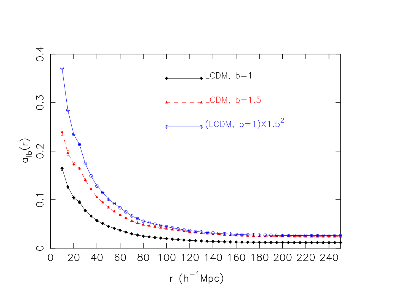
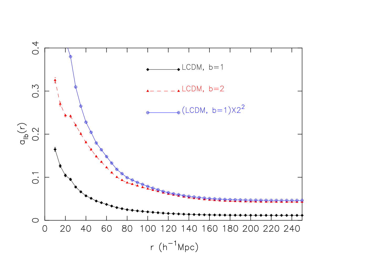
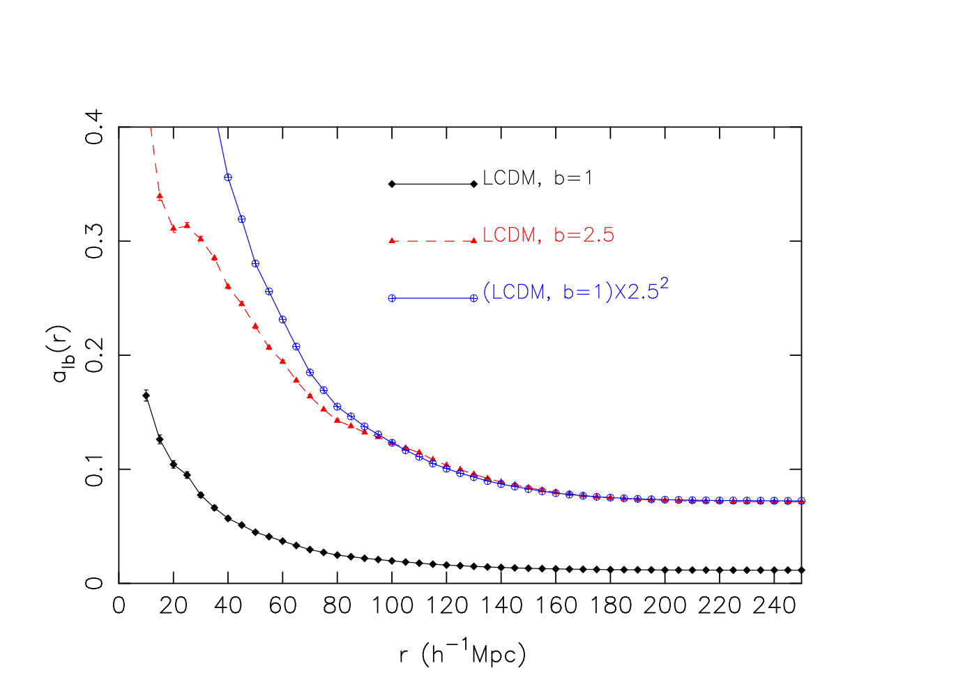
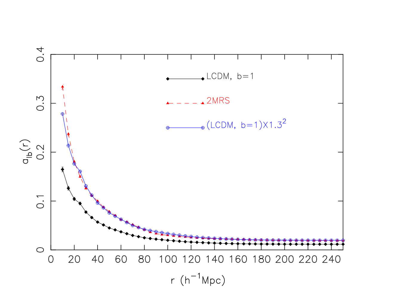
In Figure 4 we compare the radial anisotropies in the simulated mock biased galaxy samples with that from the mock samples from the dark matter distribution in the CDM model. The top left panel, top right panel and the bottom left panel of Figure 4 show the comparisons for linear bias values , and respectively. We see in each of these panels that scaling the radial anisotropy with where is the linear bias parameter of the simulated galaxy sample, reproduces the actual radial anisotropies observed in the respective galaxy samples on large scales. However this scaling shows a large deviation on small scales which gradually decreases and finally merges with the observed radial anisotropies in the biased samples beyond a length scale of . We do not expect the linear biasing to hold on small scales. On small scales, the differences result from the non-linearities present on those scales due to the gravitational clustering. The contributions from the higher order moments of the probability distribution in Equation 3 are not negligible on smaller scales and the bias values obtained by using Equation 6 are expected to deviate from its actual value. Eventually the assumption of linear bias may prevail on some larger scale and the Equation 6 can faithfully recover the linear bias values only on a scale where the non-linearity becomes negligible. In the bottom right panel of Figure 4 we compare the radial anisotropies in the 2MRS galaxy sample with that expected from the unbiased CDM model. Interestingly, when we scale the radial anisotropies in the unbiased CDM model by we find that it nicely represents the radial anisotropies observed in the 2MRS galaxy sample for nearly the entire length scales beyond . This indicates that the non-linearity becomes less important in the 2MRS galaxy sample beyond a length scale of . It is also interesting to note that though the radial anisotropy in all the biased galaxy distributions decreases with increasing length scales, they reach a plateau at different length scales. We note that for , , and the plateaus are reached at , , and respectively. This indicates that the signatures of anisotropy may persist up to different length scales depending on the bias of the galaxy distribution.
| Sample | Bias from | Bias from |
|---|---|---|
| CDM, | ||
| CDM, | ||
| CDM, | ||
| CDM, | ||
| 2MRS |
Our scheme maintains equal area for all the pixels by uniformly binning and . This causes the shapes of the pixels to vary across different parts of the sky. These variations may contribute to the anisotropies measured in our scheme. To assess this we carry out some tests with HEALPix (Górski et al., 1999; Górski et al., 2005) which uses equal area and nearly same shape for all the pixels. We calculate the radial anisotropy in the same datasets using NSide in HEALPix which provides a total pixels on the sky. It may be noted that we use and in our scheme which results into a total pixels. We find that HEALPix pixelization gives exactly the same radial anisotropy as measured in our scheme (Pandey, 2017).
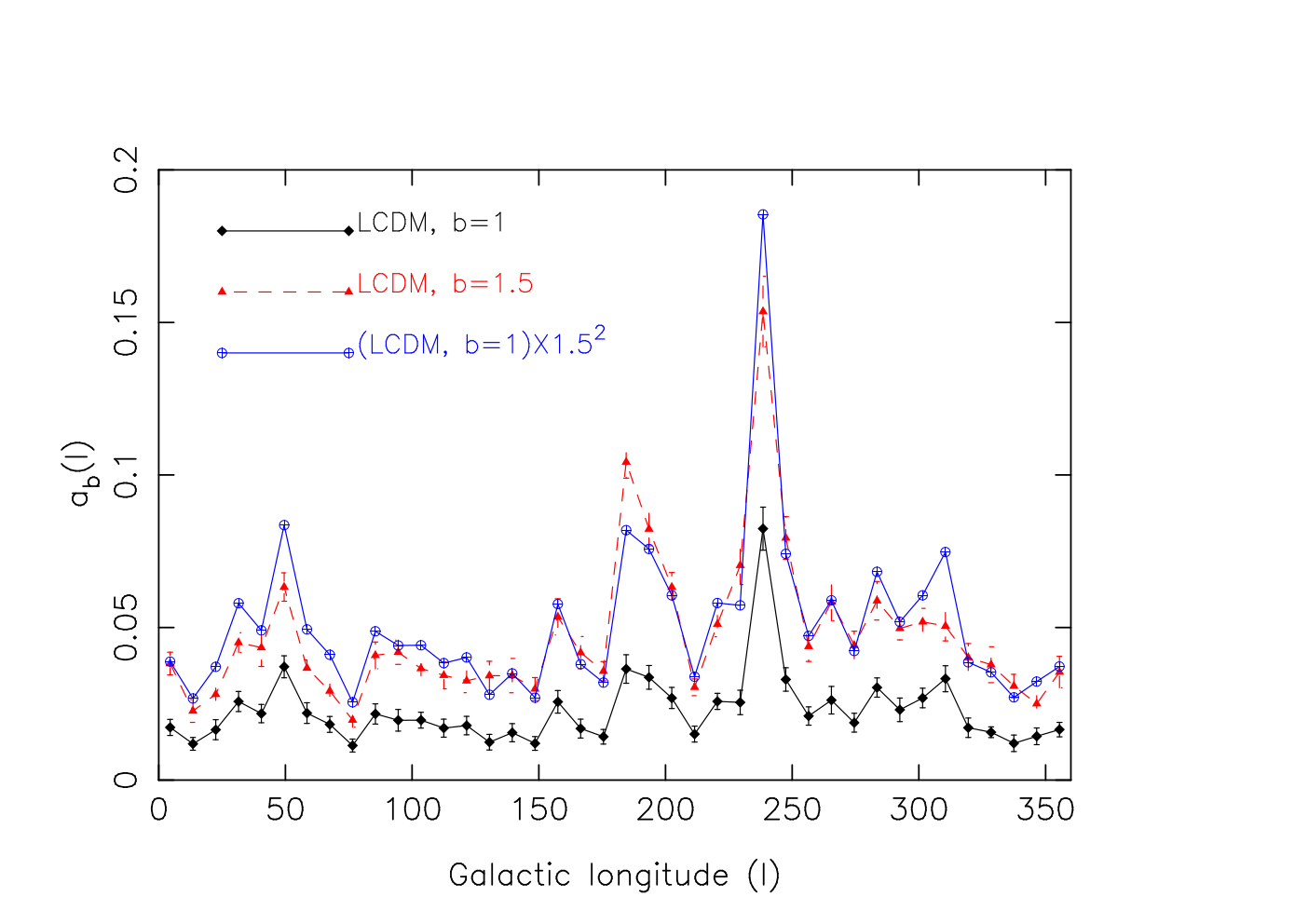
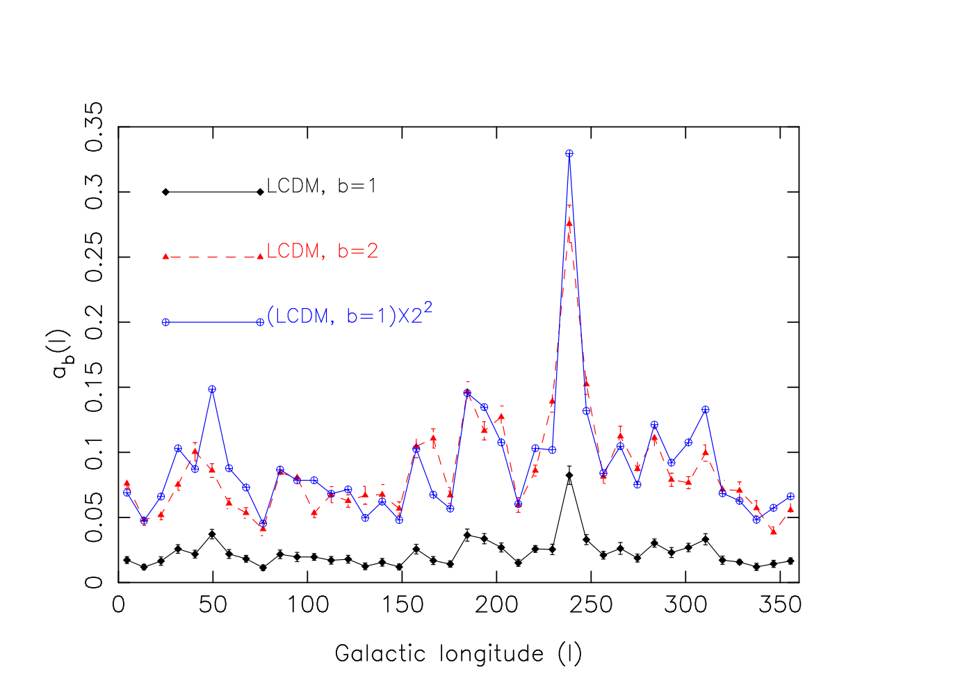
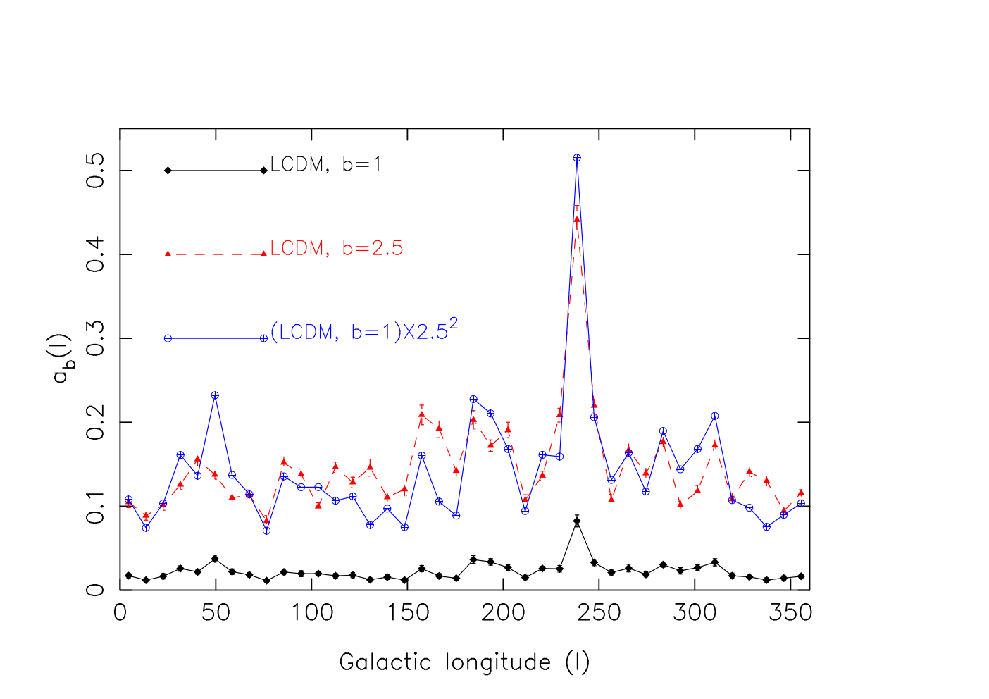
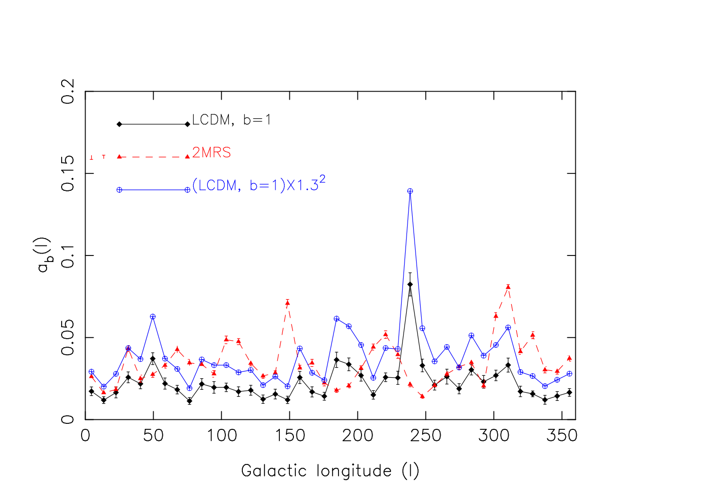
We compare the polar and azimuthal anisotropies in the biased and unbiased samples in the top left, top right and bottom left panels of Figure 5 and Figure 6 respectively. We notice that a scaling similar to Figure 4 also applies here despite the fact that a smaller number galaxies are used to compute the anisotropies at each and . It may be noted that the peaks and troughs in the polar and azimuthal anisotropy curves for the simulated samples appear nearly at the same and values as the biased distributions are produced from the same unbiased distribution. But if we compare these results with that from a galaxy distribution, we do not expect this to happen as they represent two different statistical realizations of the density field. We find that the Equation 6 can be also used effectively with polar and azimuthal anisotropies to recover the linear bias parameter of the biased galaxy samples (Table 1). We consider the polar and azimuthal anisotropies estimated from samples in each case to measure the linear bias values using Equation 6 respectively at each latitude () and longitude (). We estimate the average linear bias values and their standard errors by combining the bias measurements over different latitudes and longitudes and list them in Table 1.
In Table 1 we see that the linear bias values recovered for the simulated galaxy samples are quite close to their actual bias values. When we apply the same method to estimate the linear bias of the 2MRS galaxy sample, we get from polar anisotropy and from azimuthal anisotropy. It is interesting to note that we get nearly the same bias value from radial, polar and azimuthal anisotropies. One can also determine the relative bias parameter between any two galaxy distributions using the same method.
We also test the applicability of this method to mock samples where the radial selection function is uniform. We randomly extract particles from spherical regions of radius from each of the biased and unbiased distributions and repeated the analysis. We find that one can recover the linear bias of the simulated galaxy samples following the same method presented in this work. This suggests that the same method can be applied to determine the linear bias parameter of the volume limited sample from different galaxy surveys.
It may be noted that the computation of the two-point correlation function and power spectrum scales as where is the number of galaxies in the sample. So the computational requirements scales very fast with the size of the sample. Use of tree algorithms or FFT can reduce this scaling to (Szapudi & Szalay, 1998; Pen, 2003; Szapudi et al., 2005). Interestingly the method presented in this work requires a scaling of only and hence it is computationally least expensive among all the other existing methods for the determination of linear bias.
We finally note that a combined study of the radial, polar and azimuthal anisotropies in the galaxy distribution provides a powerful new alternative to measure the linear bias parameter from galaxy distributions.
5 Acknowledgement
The author thanks an anonymous reviewer for the valuable comments and suggestions. The author would like to thank the 2MRS team for making the data public. The author acknowledges financial support from the SERB, DST, Government of India through the project EMR/2015/001037. I would also like to acknowledge IUCAA, Pune and CTS, IIT, Kharagpur for providing support through associateship and visitors programme respectively.
References
- Alonso et al. (2015) Alonso, D., Salvador, A. I., Sánchez, F. J., et al. 2015, MNRAS, 449, 670
- Blake & Wall (2002) Blake, C., & Wall, J. 2002, Nature, 416, 150
- Briggs et al. (1996) Briggs, M. S., Paciesas, W. S., Pendleton, G. N., et al. 1996, ApJ, 459, 40
- Cole, Hatton & Weinberg (1998) Cole, S., Hatton, S., Weinberg, D. H., & Frenk, C. S. 1998, MNRAS, 300, 945
- Colles et al. (2001) Colles, M. et al.(for 2dFGRS team) 2001,MNRAS,328,1039
- Dekel & Rees (1987) Dekel A., Rees M. J. 1987,Nature,326,455
- Erdoǧdu et al. (2006b) Erdoǧdu, P., Lahav, O., Huchra, J. P., et al. 2006, MNRAS, 373, 45
- Erdoǧdu et al. (2006a) Erdoǧdu, P., Huchra, J. P., Lahav, O., et al. 2006, MNRAS, 368, 1515
- Feldman et al. (2001) Feldman, H. A., Frieman, J. A., Fry, J. N., & Scoccimarro, R. 2001, Physical Review Letters, 86, 1434
- Gaztañaga et al. (2005) Gaztañaga, E., Norberg, P., Baugh, C. M., & Croton, D. J. 2005, MNRAS, 364, 620
- Gupta & Saini (2010) Gupta, S., & Saini, T. D. 2010, MNRAS, 407, 651
- Fixsen et al. (1996) Fixsen, D. J., Cheng, E. S., Gales, J. M., et al. 1996, ApJ, 473, 576
- Górski et al. (1999) Gorski, K. M., Wandelt, B. D., Hansen, F. K., Hivon, E., & Banday, A. J. 1999, arXiv:astro-ph/9905275
- Górski et al. (2005) Górski, K. M., Hivon, E., Banday, A. J., et al. 2005, ApJ, 622, 759
- Hamilton (1992) Hamilton, A. J. S. 1992, ApJ Letters, 385, L5
- Hawkins et al. (2003) Hawkins, E., et al.2003, MNRAS,346,78
- Hazra & Shafieloo (2015) Hazra, D. K., & Shafieloo, A. 2015, JCAP, 11, 012
- Huchra et al. (2012) Huchra, J. P., Macri, L. M., Masters, K. L., et al. 2012, ApJS, 199, 26
- Kaiser (1984) Kaiser, N. 1984, ApJ Letters, 284, L9
- Kaiser (1987) Kaiser, N. 1987, MNRAS, 227, 1
- Lin et al. (2016) Lin, H.-N., Wang, S., Chang, Z., & Li, X. 2016, MNRAS, 456, 1881
- Lynden-Bell et al. (1989) Lynden-Bell, D., Lahav, O., & Burstein, D. 1989, MNRAS, 241, 325
- Meegan et al. (1992) Meegan, C. A., Fishman, G. J., Wilson, R. B., et al. 1992, Nature, 355, 143
- Marinoni et al. (2012) Marinoni, C., Bel, J., & Buzzi, A. 2012, JCAP, 10, 036
- Norberg et al. (2001) Norberg, P., et al. 2001, MNRAS, 328, 64
- Pandey (2016a) Pandey, B. 2016, MNRAS, 462, 1630
- Pandey (2016b) Pandey, B. 2016, MNRAS, 463, 4239
- Pandey (2017) Pandey, B. 2017, Accepted in MNRAS, arXiv:1703.01184
- Peebles (1980) Peebles, P. J. E. 1980, The large scale structure of the Universe. Princeton, N.J., Princeton University Press, 1980, 435 p.,
- Pen (2003) Pen, U.-L. 2003, MNRAS, 346, 619
- Planck Collaboration et al. (2016) Planck Collaboration, Ade, P. A. R., Aghanim, N., et al. 2016, A&A, 594, A13
- Scharf et al. (2000) Scharf, C. A., Jahoda, K., Treyer, M., et al. 2000, ApJ, 544, 49
- Shannon (1948) Shannon, C. E. 1948, Bell System Technical Journal, 27, 379-423, 623-656
- Smoot et al. (1992) Smoot, G. F., Bennett, C. L., Kogut, A., et al. 1992, ApJ Letters, 396, L1
- Szapudi & Szalay (1998) Szapudi, I., & Szalay, A. S. 1998, ApJ Letters, 494, L41
- Szapudi et al. (2005) Szapudi, I., Pan, J., Prunet, S., & Budavári, T. 2005, ApJ Letters, 631, L1
- Tegmark et al. (2004) Tegmark, M., et al. 2004, ApJ, 606, 702
- Verde et al. (2002) Verde, L., Heavens, A. F., Percival, W. J., et al. 2002, MNRAS, 335, 432
- Wilson & Penzias (1967) Wilson, R. W., & Penzias, A. A. 1967, Science, 156, 1100
- Wu et al. (1999) Wu, K. K. S., Lahav, O., & Rees, M. J. 1999, Nature, 397, 225
- York et al. (2000) York, D. G., et al. 2000, AJ, 120, 1579
- Zehavi et al. (2011) Zehavi, I., Zheng, Z., Weinberg, D. H., et al. 2011, ApJ, 736, 59