A semidiscrete version of the Citti-Petitot-Sarti model as a plausible model for anthropomorphic image reconstruction and pattern recognition
In his beautiful book [66], Jean Petitot proposes a sub-Riemannian model for the primary visual cortex of mammals. This model is neurophysiologically justified. Further developments of this theory lead to efficient algorithms for image reconstruction, based upon the consideration of an associated hypoelliptic diffusion. The sub-Riemannian model of Petitot and Citti-Sarti (or certain of its improvements) is a left-invariant structure over the group of rototranslations of the plane. Here, we propose a semi-discrete version of this theory, leading to a left-invariant structure over the group , restricting to a finite number of rotations. This apparently very simple group is in fact quite atypical: it is maximally almost periodic, which leads to much simpler harmonic analysis compared to Based upon this semi-discrete model, we improve on previous image-reconstruction algorithms and we develop a pattern-recognition theory that leads also to very efficient algorithms in practice.
This research has been supported by the European Research Council, ERC StG 2009 “GeCoMethods”, contract n. 239748, by the iCODE institute (research project of the Idex Paris-Saclay), by the SMAI project “BOUM”, and by the Grant ANR-15-CE40-0018 of the ANR. This research benefited from the support of the “FMJH Program Gaspard Monge in optimization and operation research” and from the support to this program from EDF.
This book contains, among others, results from [10, 13, 42]. For their kind permission to reproduce parts of these papers we thank the Society for Industrial and Applied Mathematics and Springer-Verlag.
Paris, Toulon, Dario, Prandi
April 2017 Jean-Paul Gauthier
Chapter \thechapter Introduction
1 Neurophysiological considerations and the Citti-Petitot-Sarti model
The primary visual cortex V1 is a (not small) part of the brain, whose location is shown on Figure 1. It is responsible, after the retina, for elementary representations of the visual field, by visual charts, that take into account not only position, but also orientation.
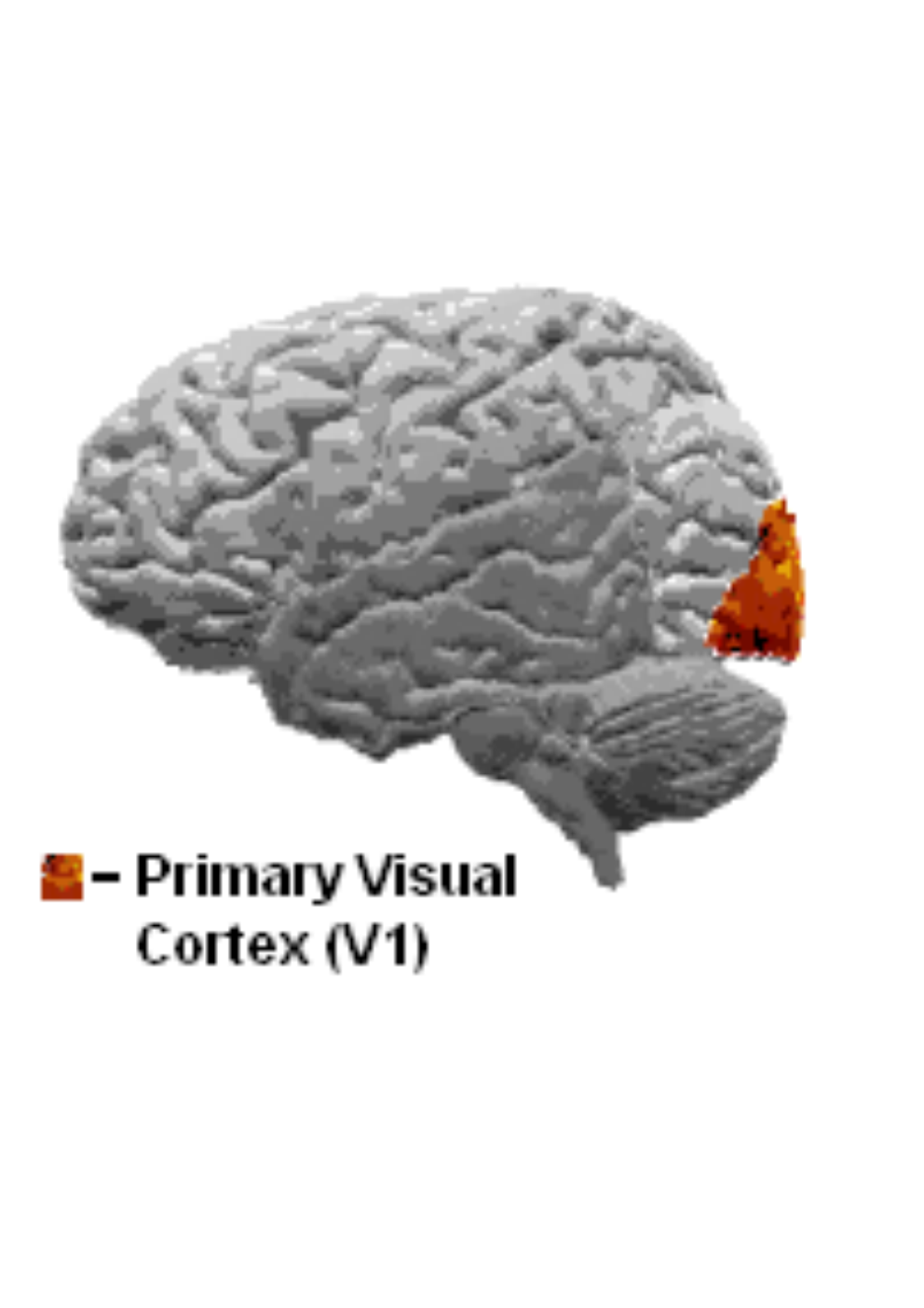
In the paper [67] and his beautiful book [66], Jean Petitot describes a sub-Riemannian model of the visual cortex V1. The main idea goes back to the paper by Hübel an Wiesel in 1959 (Nobel prize in 1981) [52] who showed that in the visual cortex V1, there are groups of neurons that are sensitive to position and directions with connections between them that are activated by the image. The key fact is that the system of connections between neurons, which is called the functional architecture of V1, preferentially connects neurons detecting alignments.
Roughly speaking, neurons of V1 are grouped into orientation columns, each of them being sensitive to visual stimuli at a given point of the retina and for a given direction on it. Orientation columns are themselves grouped into hypercolumns, each of them being sensitive to stimuli at a given point with any direction (see Figure 3).

In the visual cortex there are two types of connections: the vertical connections among orientation columns in the same hypercolumn, and the horizontal connections among orientation columns belonging to different hypercolumns and sensitive to the same orientation. For an orientation column it is easy to activate another orientation column which is a “first neighbor” either by horizontal or by vertical connections. This is the so-called pinwheels structure of V1. (See Figures 2 and 3.) Pinwheels are the locations where multiple orientation columns converge. Orientation columns are organized radially around a point known as a singularity. As one can check on Figure 2, there are both clockwise and counterclockwise oriented pinwheels.

From the mathematical point of view, it is thus assumed that V1 lifts the images (i.e., functions of two position variables in the plane of the image) to functions over the projective tangent bundle This bundle has as base and as fiber over the point the set of directions of straight lines lying on the plane and passing through .
Consider for instance the simplest case in which the image is a smooth curve Lifting this curve to means to add a new variable that is the angle of the vector . Since we are obliged at some point to go to certain stochastic considerations, it is convenient to write this lift in the following “control form”. We say that ··· is the lift of the curve ·· if there exist two functions · and · (called controls) such that
| (1) |
Here the control plays the role of the modulus of the planar vector , but can take positive and negative values since the angle is defined modulo . The control is just the derivative of .
Remark 1
. The vector distribution , where and is a vector distribution that endows with the structure of a contact manifold. Indeed is completely non-integrable (in the Frobenius sense) since and satisfy the Hörmander condition: for each
Notice that the definition of vector field is not global over since it is not continuous at : the distribution is not trivializable and a correct definition of it would require two charts. However, for sake of simplicity, we proceed with a single chart with some abuse of notation. Notice, however, that if we lift the problem to the group SE(2) of rototranslations of the plane, which is a double covering of , the structure becomes trivializable and the definition of becomes global. We do this often along the paper. We will just underline places where the projectivization comes in and is important.
In the model described by Petitot, when a curve is partially interrupted, it is reconstructed by minimizing the energy necessary to activate the regions of the visual cortex that are not excited by the image.
Since for an orientation column it is easy to activate another orientation column which is a “first neighbor” either by horizontal or by vertical connections, following Petitot, the energy necessary to activate a path is given by
| (2) |
Here, the term is proportional to the energy necessary to activate horizontal connections, while the term is proportional to the energy necessary to activate vertical connections. The parameter is a relative weight.
To conclude, in V1, the problem of reconstructing a curve interrupted between the boundary conditions and becomes the optimal control problem:
| (12) | ||||
| (13) | ||||
| (14) |
Finding the solution to this optimal control problem can be seen as the problem of finding the minimizing geodesic for the sub-Riemannian structure over defined as follows: The distribution is and the metric over is the one obtained by claiming that the vector fields and form an orthonormal frame.
By construction this sub-Riemannian manifold is invariant under the action of the group of rototranslations of the plane. Indeed, are the only sub-Riemannian structures over which are invariant under the action of . See for instance [1].
Remark 2
From the theoretical point of view, the weight parameter is irrelevant: for any there exists a homothety of the -plane that maps geodesics of the metric with the weight parameter to those of the metric with . For this reason, in all theoretical considerations we fix . However its role will be important in our image reconstruction algorithms.
Remark 3
The history of this model goes back to the paper by Hoffman [51] in 1989, who first proposed to regard the visual cortex as a manifold with a contact structure. In 1998, Petitot [67, 66] wrote the first version of the model as a constrained minimization problem on the Heisenberg group and gave an enormous impulse to the research on the subject. In 2006, Citti and Sarti [23] required the invariance under rototranslations, and wrote the model on , recognizing it as a sub-Riemannian structure and explicitly introducing the vector fields . In [15], it was proposed to write the problems on to avoid some topological problems and to be more consistent with the fact that the visual cortex V1 is sensitive only to directions (i.e., angles modulo ) and not to directions with orientations (i.e., angles modulo ). The theory was wonderfully completed in Petitot’s book [66].
The detailed study of geodesics was performed by Yuri Sachkov in a series of papers [69, 70]. For modifications of the model aimed to avoid the presence of geodesics whose projection on the plane has cusps, see [23, 72, 11, 14]. This model was also deeply studied by Duits et al. in [31, 34], with medical imaging applications in mind, and by Hladky and Pauls [50]. Of course this model is closely related with the celebrated model by Mumford [62]. See also [4, 7].
The model described by Petitot was used to reconstruct smooth images by Ardentov, Mashtakov and Sachkov [60]. The technique developed by them consists of reconstructing as minimizing geodesics the level sets of the image where they are interrupted.
When applying the above strategy to reconstruct images with large corrupted parts, one is faced to the problem that it is not clear how to put in correspondence the non-corrupted parts of the same level set. For this reason, in [15, 34], was proposed the following method. In system (1), excite all possible admissible paths in a stochastic way, obtaining the SDE:
| (16) |
where are two independent Wiener processes. To this SDE is naturally associated a diffusion process (here we have fixed ):
| (17) | ||||
The operator is not elliptic, but it is hypoelliptic (indeed it satisfies the Hörmander condition). By the Feynman–Kac formula, integrating Equation 17 with the corrupted image as the initial condition, one expects to reconstruct the most probable missing level curves (among admissible).
Remark 4
Note that the operator is the intrinsic sub-Riemannian Laplace operator over the (unimodular) group , as defined in [2].
To summarize, in this model, the process of reconstruction by V1 of corrupted images is the following
- •
The plane image is lifted to a certain “function” on the bundle
- •
The diffusion process (17) with the initial condition is integrated on the interval for some .
- •
The resulting function on the bundle is projected down to a function , which represents the reconstructed image.
The lifting procedure should be as follows: the image is assumed to be a smooth function . Then, it can be naturally lifted to a surface in by lifting its level curves11 1 It is widely accepted that the retina performs some smoothing, see [57]. After such smoothing, the image is in general a Morse function, and the lifted surface is a smooth surface. See [15].. At a point we would like to set if and elsewhere. But this would be nonsense since has zero measure in Hence, is lifted to a distribution , supported in , and weighted by . We refer to [15] for details.
The idea of modeling the process of reconstruction of images in V1 as an hypoelliptic diffusion was presented first in [23] and was implemented in details with various modifications and different purposes by many authors. See, e.g., [72, 15, 30, 34, 22, 81] and references therein. A clever variant to the lifting process, which inspired the left-invariant lifts used in this work, was proposed in [34, 35].
It turns out that although good looking, Equation (17) is not easy to integrate numerically. In particular, the multiscale sub-Riemannian effects are hidden inside. (The numerical literature for PDEs in sub-Riemannian geometry appears to be very scarce.)
For the equation (17) it is possible to compute the associated heat kernel, see [2, 30, 34]. See also [80] for a review on its numerical implementations. Moreover, the numerical integration starts to be a rather large problem, due to the number of points/angles in a reasonable image.
Some promising results about inpainting using hypoelliptic diffusion were obtained in [15]. In this paper a reasonable algorithm is presented. This algorithm is recalled here, with some improvements. See also [13].
To end this section, we mention that the initial purpose of the aforementioned algorithms was the so-called “modal” reconstruction. (See Figure 4.) That is, the reconstruction of contours that are actually perceived by the observer. However, the results obtained, especially those of [13], show that these algorithms can be used also for “amodal” completions. This term designates the completion via a mental extrapolation of contours that are not visible by the observer. Since some of the results are uncanny with respect to what a human observer can do, this suggests that this model, although very efficient in practice, is not a completely realistic neurophysiological model.


2 Our semi-discrete model
We shall use certain elementary and non elementary facts from representation theory of locally compact groups. For general representation theory see the book of Dixmier [27] or [8, 78, 19]. For a detailed treatment of see [76]. Almost periodic functions and Bohr compactification will also be important here. See again [27] and [79, 24]. We also need standard results on duality theory for locally compact groups. Recall that compact groups are subject to Tannaka duality (an avatar of Pontryagin duality on abelian groups). Here, we will consider maximally almost-periodic (MAP) groups, which are subject to Chu duality, a generalization of Tannaka duality. For Chu duality, see the foundational paper of Chu [21] and the book by H. Heyer [48].
In the Petitot model, we assume a finite number of columns in the hypercolumns. Moreover, this number is assumed to be rather small22 2 Looking at the literature, discussing with Petitot and other people, we could not get a clear answer about this number N. This estimate (15 to 50) comes from our own numerical experiments in both image reconstruction and pattern recognition. (between 15 and 50). It corresponds to a small number of directions on and a small number of angles on the double-covering Then, we are naturally led to the consideration of the (semi-discrete) subgroup of rigid motions, corresponding to rotations with angles ( integer). This group is denoted by It is the semi-direct product of the finite abelian group by It is a very interesting group that we will study in details, together with some of its (finitely generated) subgroups. We also mention that this group has already been used in various image processing papers, e.g., [74, 23, 29].
The semi-discrete group of Euclidean motions turns out to have quite a rich structure: although non-compact, it is a MAP group and, even more, it is a Moore group, i.e. all its unitary irreducible representations are finite dimensional. Since, just as , it is a semi-direct product, these representations can be computed by using Mackey’s machinery (see [59, 8], but we shall recall precisely what we need in the paper).
In the paper, we treat two questions that investigate the way V1 performs image reconstruction of corrupted images, and also (this is our conjecture) the way V1 computes some important quantities that are used at a higher level in the brain, to perform planar pattern recognition. For both purposes the structure of is crucial.
We already explained how in the (continuous) Petitot model image reconstruction is performed by lifting to and integrating a certain hypoelliptic Laplace operator (see Remark 4 above).
Usual Fourier transform diagonalizes the usual Laplace operator. Similarly, the generalized Fourier transform [27] over disintegrates our sub-Riemannian Laplace operator into a continuous sum of Mathieu-type operators. At the level of the same scenario appear: A semi-discrete Laplacian comes in the picture, and it is again disintegrated by Fourier transform over into a (continuous) sum of finite dimensional (Mathieu-like) linear operators. In particular, the corresponding heat kernel has a simple explicit expression. From these considerations, we derived interesting numerical methods for the problem of completion of images.
3 Textures
We are led to consider as models for textures, certain (sometimes finite dimensional) subspaces of the space of Besicovitch almost periodic functions (see [24]). Approximation and interpolation of usual images by elements of these texture spaces (adapted to the structure of ) is an interesting problem in itself, to which we provide a reasonable solution.
This representation is crucial in our work, since it is deeply used in both problems treated herein, i.e image reconstruction and pattern recognition. In fact, these very natural finite dimensional subspaces are (roto)translation invariant over Moreover, the unitary irreducible representations of act on some of these spaces . This leads to very reasonable algorithms for both image reconstruction and pattern recognition. In particular, over these spaces, the semi-discrete diffusion becomes just a linear ordinary differential equation.
Moreover, we remark that such representation is of interest in itself due to its close relation with the Fast Fourier Transform algorithm, with the problem of the ”polar” Fourier transform [5], and more generally with the non-uniform FFT, about which there is an important amount of literature. We give just a small non-exhaustive list of references: [6, 17, 36, 58, 64, 65, 68]. This is in particular an important question in the fields of NMR and computed tomography.
4 Triple convolution and bispectrum
For real valued functions over , the auto-correlation and the triple correlation (or triple convolution) are
Denoting by the usual Fourier transform of , it is easily computed that the Fourier transform is just the power spectrum (Here * stands for conjugate).
Also, the Fourier transform (over of the triple correlation is what is called the Bispectrum of :
The bispectrum (or equivalently the triple convolution) is translation-invariant, and is used for long in many areas of signal processing ([44, 40, 54, 53]). It was also used for texture discrimination of music instruments (see [28]) an it is suspected that the auditive cortex proceeds with bispectra.
These invariants already appeared in pattern recognition. They are alternatively called Fourier descriptors (see [10, 74, 41]). In these papers, a natural abstract generalization on locally compact groups is proposed. For a locally compact group and , with being the Haar measure, the bispectrum of is the operator valued map:
| (18) |
where are unitary irreducible representations of and * denotes the adjoint operator. Bispectra are clearly invariant w.r.t the action of translations of . The main fact is that they are highly discriminating between functions up to translations.
Let us say that a set of translation-invariants is weakly complete if it discriminates between functions modulo the action of translations, over a residual subset of It turns out that, when is abelian, compact (separable), or MAP, the bispectra are weakly complete. This is the main fact, and the residual subset of functions over which bispectra discriminate is just the set of such that the Fourier transform is an invertible operator.
Hence, the idea is very simple: to discriminate between images on the plane, i.e. functions let us, as for image reconstruction, lift the functions to functions over and compute the bispectral invariants of (We mention that different pipelines are possible, see, e.g., [73].) After this step, we would like to feed a learning machine (such as an SVM machine [75]), or a deep learning machine, with the lifted bispectra We expect to get very good performances for pattern recognition [74].
Our (plausible?) expectation is that the primary visual cortex feeds higher level strata of the brain with such invariants.
Unfortunately, a very bad feature appears: if we require (which is natural) the lift to be left-invariant, the Fourier transform of is never invertible (on the contrary, it has always rank at most one). Therefore, we do not know whether bispectral invariants are weakly complete over or not.
A long piece of this monograph has for purpose to overcome this difficulty. Roughly speaking, we need the extra ingredient of ”centering” the images (which can be done with respect to the gravity center of the image for images, but which is not so easy in the case of almost periodic functions). The purpose of this centering procedure is to eliminate the effect of translations. After this centering, we define quite naturally another set of invariants, richer than the bispectrum, that we call rotational bispectral invariants. They make sense for both cases of images in and for our texture spaces As a last step, we are able to derive weak completeness results.
5 Organization of the paper
The second chapter introduces all the technical tools and concepts we need, i.e. general facts about locally compact groups, the non-commutative Fourier transform and general Plancherel’s theorem, Chu duality. We introduce our centering operators, we recall the main facts of Mackey’s imprimitivity theory, together with the induction-reduction theorem for the decomposition of tensor products of induced representations. We define weakly cyclic functions, and we discuss a (more or less standard) version of the abstract wavelet transform, that will be useful in our lifting process.
We define Bohr compactification, Bohr and Besicovitch almost periodic functions and our relevant subspaces of almost periodic functions. We discuss the process of centering almost periodic functions.
Chapter 3 discusses the lifting problem, mainly from to or . In fact, we do it in a slightly more general context. We show first that continuous left invariant lifts are essentially wavelet transforms, and we characterize injectivity of the lifts. We then show that Fourier transforms of (left-invariant) lifted functions have always rank one. To finish, we define almost left-invariant lifts and cyclic lifts, that will be enough for our discrimination purposes.
Chapter 4 deals with almost periodic interpolation and approximation. As we said in the introduction (Section 3), this chapter is interesting in itself. It is strongly related with the problems of non-uniform FFT and polar FFT. We define a generalized Fourier-Bessel operator, and we prove a factorization theorem for this operator. This factorization theorem is the key point for the algorithms of evaluation, interpolation, approximation of functions in our texture spaces
Chapter 5, Pattern Recognition, is the heart of the paper. Bispectral invariants are defined in general by formula (18). We prove the main discrimination result over abelian, compact and Moore groups. Next, we treat the problem of discriminating lifted functions. First, we define cyclic lifts and provide a proof of weak completeness in that case. The remaining of the chapter studies our rotational bispectral invariants in view of weak completeness.
In Chapter six, we focus on the image reconstruction problem, recalling previous results and providing some improvements in the case of We construct the heat operator in the case of via elementary stochastic considerations and we recall the expressions of the heat Kernels in both cases of and . We present the basic completion algorithm, and we show how it works in the case of our spaces of almost periodic functions, in which case it just relies on integrating linear ordinary differential equations (a finite number of them, provided that is finite).
Chapter 7 is about applications. First we care about image reconstruction, and we show how our basic algorithm can be substantially improved on by certain natural heuristic considerations. We show some very convincing reconstruction results. However these results provide very little improvement w.r.t. the state-of-the-art, which actually consists of extremely efficient algorithms. (See, e.g., [37, 18].) Therefore, our main contribution here is not over this practical area. In fact we just “validate” the Citti-Petitot-Sarti model and our semi-discrete improvement of it. Moreover, we reduce the diffusion to ODE’s which is conceptual gain only.
Second, we care about pattern recognition. On the contrary, in this area we get very interesting practical results, with several advantages w.r.t. some other standard methods. The basic idea, as we said, is to feed a learning machine with our bispectral invariants. These invariants have a number of good features for discrimination: they are continuous invariants (which is absolutely necessary) and they rely on the consideration of a set of basic frequencies (over the frequency plane). Depending on the application, it is quite an easy routine to select properly this set , that in some situations has a clear frequency interpretation. Moreover, this approach allows rather easily to pass to 3D pattern recognition. Roughly speaking, it is enough to feed the learning step with a number of pictures of the object under consideration, taken under several distinct points of view.
To test our invariants, we chose to use the SVM learning machine by V. Vapnik [75], and some of its improvements. We remark, however, that we could have chosen a more fashionable deep learning machine. On the web, one can find easily a series of test data, results and procedures in order to perform comparisons with other methods. We present some of these comparisons, mostly from our papers [74, 10].
To finish, we insist on the fact that the main interest (from the image processing point of view) of this semi-discrete model (i.e., the lift of images to functions over ) is not image completion but pattern recognition.
Chapter \thechapter Preliminaries
This chapter introduces the concepts that are the main subject of the rest of this work, along with the essential tools that are needed. After a brief introduction on harmonic analysis in non-commutative groups, we introduce the general setting considered in this work, alongside with some essential facts on its representation theory. Afterwards, we recall some basic notions on almost-periodic functions and and a precise construction that allows to select some relevant subspaces. Finally we present our models for natural images (compactly supported functions of ) and textures (properly selected finite-dimensional subspaces of almost-periodic functions in the plane).
6 Prerequisites
In the following, we briefly recall some well-known fact in commutative and non-commutative harmonic analysis. In particular, we introduce the Fourier transform and the Plancherel theorems that will be the basis of our work.
6.1 Conventions
Scalar products on complex-valued vectors or functions of an Hilbert space are always assumed to be linear in the second variable. According to this convention, the tensor product of is the linear operator
| (19) |
That is, .
6.2 Harmonic analysis on locally compact abelian groups
Let be a locally compact abelian group with additive notation. A character of is a continuous group homomorphism such that for any . Defining the product of two characters as the point-wise multiplication and the inverse as the complex conjugation, the set
| (20) |
endowed with the topology of uniform convergence on compact sets, is a locally compact abelian group, called the (Pontryagin) dual group of .
It is straightforward to check that defined by , is a continuous group homomorphism. In particular, .
Theorem 6.1 (Pontryagin duality)
The map is a group isomorphism, and thus is canonically isomorphic to the dual of .
The Fourier transform allows to carry the above isomorphism to the level of complex-valued functions defined on and . Namely, endow with its Haar measure and for any define its Fourier transform by
| (21) |
Observe, in particular, that letting it holds , where is the identity of . We have the following.
Theorem 6.2 (Plancherel Theorem)
There exists a unique measure on , called Plancherel measure, such that the above defined Fourier transform can be extended to an isometry . In particular, whenever and , it holds that
| (22) |
Remark 5
When the above procedure yields the classical Fourier transform. Indeed, the Haar measure of is the Lebesgue measure, can be realized as the set of for , and the Plancherel measure is the normalized Lebesgue measure.
The left regular representation of is the map defined as . Then, the fundamental property of the Fourier transform, at least for our purposes, is the following.
Theorem 6.3
For any and any it holds that
| (23) |
6.3 Fourier transform on locally compact non-commutative groups
Let be a locally compact unimodular group, not necessarily abelian. A unitary representation of is a continuous33 3 With respect to the strong topology of . Recall that this is not the norm topology, w.r.t. which irreducible representations are not in general continuous. homomorphism , where is a complex (possibly infinite dimensional) Hilbert space. A representation is irreducible if no nontrivial closed subspace of is invariant for all , . Two representations and are equivalent if there exists a linear invertible operator such that . In this case we write .
The dual set of is the set of all equivalence classes of unitary irreducible representations of . Although, for abelian, the only irreducible representations are the characters, and this set coincides with the Pontryagin dual, in the general case it has no group structure. The Fourier transform of a function is then defined by
| (24) |
Observe that is a Hilbert-Schmidt operator on .
Remark 6
The same formula can be used to define the values of on not necessarily irreducible unitary representation of .
We have the following generalization of Theorem 6.4.
Theorem 6.4 (Unimodular non-commutative Plancherel Theorem)
Let be a locally compact separable unimodular group. Then, there exists a (unique) Plancherel measure on such that the above definition can be extended to an isometry . In particular, the following inversion formula holds
| (25) |
As in the abelian case, the Fourier transform has a nice behavior w.r.t. to the action of the left regular representation , defined by , as shown in the following.
Theorem 6.5 (Fundamental property w.r.t. the action of the left regular representation)
For any and any it holds
| (26) |
6.4 Chu Duality
Chu duality is an extension of the dualities of Pontryagin (see Theorem 6.1) and Tannaka (for compact groups) to a class of more general groups. In particular, it applies to Moore groups, i.e., those groups whose unitary irreducible representations are all finite dimensional. Here, the difficulty is to find a suitable notion of bi-dual, carrying a group structure. See [47].
Let denote the set of continuous unitary representations of over . Taking as a basis of neighborhoods at the sets
| (27) |
for and compact, the set is a topological space which turns out to be locally compact since is so. The Chu dual of is the topological sum
| (28) |
A quasi-representation of is a continuous map from to such that for any , , and it holds
- 1.
;
- 2.
;
- 3.
;
- 4.
;
The set of quasi-representations of is denoted by and is called the Chu quasi-dual. Setting and , the Chu quasi-dual is an Hausdorff topological group with identity . Finally, we can define the continuous group homomorphism as
| (29) |
Definition 1
A locally compact group has the Chu duality property if is a topological group isomorphism.
The main result is then the following.
Theorem 6.6
Any Moore group has the Chu duality property.
Observe that, since all abelian and/or compact groups are Moore, Chu duality contains both Pontryagin and Tannaka duality.
7 General setting
We now present the general setting that we will consider for most of this work, that of certain semi-direct product groups. We also recall some well-known facts regarding the corresponding representation theory.
Let us consider the semi-direct product , obtained thanks to the action . We will always assume the following:
- •
is an abelian separable connected locally compact group.
- •
is an abelian finite group of cardinality .
- •
The restriction of the action to is free.
- •
The Haar measure of is invariant under the ’s.
The above assumptions guarantee that is unimodular (63, Ch. II, Prop. 28). Note that is also automatically post-liminal. Later on we will explicitly compute the unitary irreducible representations of , which will be finite dimensional, thus proving that is a Moore group.
Remark 7
The freeness assumption on the action of could probably be removed. However, this would yield to a more complicated description of the representations of and it is outside the scope of this work, whose main motivation is .
Additive notation is used for and multiplicative one for . We denote the identity of by and that of by . The letters are reserved for elements of , while are elements of . Elements of the Pontryagin duals and are denoted, respectively, as and . The identities of the Pontryagin duals are and . Elements of are denoted either by or as couples .
The action of on induces a contragredient action of on , still denoted and defined by . The left regular representations of and are called translation and shift operators and denoted by and , respectively. Their actions on and are given by
| (30) |
When is cyclic, i.e. , the shift operator is completely determined by via , times.
The left regular representation of is denoted by , and its action on is . Exploiting the semi-direct product structure of , we can consider the quasi-regular representation of , denoted by and whose action on is
| (31) |
The quasi-regular representation is far from being irreducible, see, e.g., [39]. Indeed, to any measurable -invariant , is associated the following closed invariant subspace
| (32) |
By conjugating the quasi-regular representation with the Fourier transform on we obtain the representation on . Since , is given by
| (33) |
Throughout the paper we will be interested in quotienting out the effect of the action of , or one of its subsets, on .
Definition 2
Let be invariant under the action of and let . A centering of w.r.t. is an operator that acts by , where is such that, for any ,
| (34) |
Observe that the above implies that for any it holds
| (35) |
It is then clear that is invariant under the action of .
7.1 Representation theory
A complete description of the unitary irreducible representations of can be obtained via Mackey machinery, see e.g., (8, Ch. 17.1, Theorems 4 and 5). We recall it in the following.
Theorem 7.1 (Representations of semidirect products)
To any corresponds the unitary representation of defined by and acting on . On the other hand, to any corresponds the unitary representation acting on and defined by
| (36) |
Moreover, the dual set is the union of the set of the nontrivial orbits in under the action of and of . Indeed, for any it holds that and hence is equivalent to whenever belong to the same orbit. Finally, the Plancherel measure is supported outside of .
Remark 8
When , the set of nontrivial orbits can be identified with the “slice of Camembert” , defined by
| (37) |
Let be the canonical basis of given by
| (38) |
Then, the coefficients of w.r.t. this basis are
| (39) |
where denotes the Kronecker’s delta. In Chapter A semidiscrete version of the Citti-Petitot-Sarti model as a plausible model for anthropomorphic image reconstruction and pattern recognition we will explicitly compute the coefficients of with respect to the dual basis and we will relate these to Bessel functions.
Proposition 1
Let . Then, for any , the components of w.r.t. the canonical basis of are
| (40) |
Moreover, for any and for any it holds
| (41) |
Here, we let be defined as
| (42) |
Proof
Since , the first statement follows by (39):
| (43) |
On the other hand, to prove the second statement it suffices to compute
| (44) |
7.1.1 Induction-Reduction theorem
Throughout the paper, we will use a well-known fact on tensor product representations: the Induction-Reduction Theorem. (See [8].) This theorem allows to decompose the tensor products of representations , acting on , to an equivalent representation acting on , which is a block-diagonal operator whose block elements are of the form . In particular, the Induction-Reduction Theorem plays the role of the Klebsch-Gordan decomposition in the non-compact case. We use it several times in our technical computations, Section 3.2 in particular, and in the proof of our main results.
Theorem 7.2 (Induction-Reduction Theorem)
For any it holds
| (45) |
In particular, the unitary equivalence is given by
| (46) |
where is the operator , .
Proof
Let be the canonical basis of . It is clear that to prove the theorem it suffices to show that, for all and , it holds
| (47) |
By (39), the right hand-side computes to
| (48) |
On the other hand, for all , it holds
| (49) |
Since a simple computation shows that , this yields
| (50) |
Finally, it is easy to check that the above coincides with (48) for all .
The action of linear operators , can be block-decomposed as
| (51) |
To be precise, , where is the projection on the on the -th component and its adjoint. Direct computations yield the following.
Proposition 2
Let be the equivalence in Theorem 7.2. Then, the following holds
- •
For any linear operator with components , the operator has block component:
(52) In particular, for a couple of linear operators it holds
(53) - •
Let be defined by for any and . Then,
(54)
7.2 Weakly cyclic functions
In this section we present the space of weakly-cyclic functions. These are functions of whose Fourier transform, evaluated on a.e. orbit in w.r.t. yields a well-behaved element of . Since all our results in pattern recognition of Chapter A semidiscrete version of the Citti-Petitot-Sarti model as a plausible model for anthropomorphic image reconstruction and pattern recognition will apply only to this class of functions, we will later show, in Section 17.2, that the generic image is indeed represented by a weakly-cyclic function.
A vector is cyclic if is a basis for . If is cyclic and finite with elements, recalling that for , this is equivalent to the following circulant operator (see Appendix A semidiscrete version of the Citti-Petitot-Sarti model as a plausible model for anthropomorphic image reconstruction and pattern recognition) being invertible
| (55) |
For we denote by the abelian Fourier transform on . From the action of on we obtain a contragredient action on , still denoted by , letting . Finally, for we let the vector be the evaluation at of the (inverse) -orbit of , that is
| (56) |
Observe that , since .
Since the vector cannot be cyclic for every , thus motivating the following definition.
Definition 3
A function is weakly cyclic if is cyclic for a.e. . We denote by the set of weakly cyclic functions.
7.2.1 Real valued functions
Our arguments in the following are heavily based on exploiting the weak-cyclicity property. However, we now show that, if satisfy an “evenness” condition, no real-valued function can be weakly-cyclic. The rest of this section is then devoted to define the concept of -weak-cyclicity, which will be exploited in Section 17.1 to circumvent this problem.
Definition 4
The action of on is even if there exists such that .
A necessary condition for the action to be even is that . The example to keep in mind is that of the natural action of on when is even, in which case .
Proposition 3
Let be acting evenly on and define the following proper -linear subspace of
| (57) |
Then, for any and any . In particular, is never cyclic.
Proof
From the evenness of the action, it follows that for any and . Using that , the statement follows from
| (58) |
Observe that is invariant under the action of the shift operator. We then say that is -cyclic if , and pose the following.
Definition 5
If the action of on is even, a real valued function is weakly -cyclic if is -cyclic for a.e. . On the other hand, if is not acting evenly on , is weakly -cyclic if it is weakly cyclic in the sense of Definition 3.
We denote by the set of weakly -cyclic functions.
Let be acting evenly on . Consider and fix any section . Define the map as
| (59) |
Obviously is invertible and -linear, and thus it endows with the structure of a real vector space. When with even, the natural choice for leads to identify with the first components of vectors in .
Since is invariant under the shifts, is a representation of acting on . Its action can be described explicitly:
| (60) |
It is then immediate to see that is -cyclic if and only if . We can then translate the -cyclicity property to vectors of . In particular, when is cyclic with elements, -cyclicity of is equivalent to the invertibility of the following “even circulant” matrix
| (61) |
7.3 Wavelet transform
We now introduce the concept of (continuous) wavelet transform. In Chapter A semidiscrete version of the Citti-Petitot-Sarti model as a plausible model for anthropomorphic image reconstruction and pattern recognition, we will observe that, under some reasonable assumptions, the operators lifting functions from to can always be seen as wavelet transforms associated with the quasi-regular representation . The following results are well-known and can be found, e.g., in [39]. (See also [38].)
Let be a strongly continuous unitary representation of a locally compact group on the Hilbert space . Given a vector , the wavelet transform of w.r.t. the wavelet is the linear bounded operator defined by
| (62) |
We call admissible if is an isometry from onto and weakly admissible if is a bounded one-to-one mapping onto .
If is a semi-direct product, it is natural to consider the wavelet transform w.r.t. the quasi-regular representation , acting on . Recall that . Straightforward computations then show that , where denotes the usual convolution product in . We will need the following observation,
| (63) |
As an immediate consequence, see [39], we have that
| (64) |
Here, is the vector defined in (56). We then have the following.
Theorem 7.3
Let . Then,
- •
is weakly admissible is strictly positive and belongs to ;
- •
is admissible it holds for a.e. .
In the sequel, we will frequently need to know the non-commutative Fourier transform of a wavelet transform , which is given in the following.
Proposition 4
Let . Then, it holds
| (65) |
Moreover, if it holds
| (66) |
Proof
By Proposition 1 and (63), we have
| (67) |
This completes the proof of the first part of the statement.
On the other hand, observe that . Indeed,
| (68) |
Thus, and for , and the second part of the statement follows from Proposition 1.
As a consequence of the Induction-Reduction Theorem we also obtain this result.
Corollary 1
Let Then, for any and any , we have
| (69) |
Here, is the equivalence from to given by the Induction-Reduction Theorem. (See Theorem 7.2.)
Proof
The statement follows from the Induction-Reduction Theorem, the fact that the Fourier transform commutes with equivalences and direct sums, and Proposition 4.
8 Almost periodic functions and MAP groups
As we already mentioned, we consider almost-periodic functions as a model for textures. In this section we introduce both Bohr and Besicovitch almost-periodic functions from the group-theoretic point of view, i.e., as the pull-back of certain functional spaces on the Bohr compactification of . We then proceed to introduce a reasonable concept of action of on Besicovitch almost-periodic functions, under which we will show in Chapter A semidiscrete version of the Citti-Petitot-Sarti model as a plausible model for anthropomorphic image reconstruction and pattern recognition how to discriminate. Finally, in Section 8.1, we introduce the finite-dimensional spaces of almost-periodic functions which will be the main object of interest in Chapter A semidiscrete version of the Citti-Petitot-Sarti model as a plausible model for anthropomorphic image reconstruction and pattern recognition. For the results in this section we refer to (27, Ch. 16).
Definition 6
The Bohr compactification of a topological group is the universal object in the category of diagrams where is a continuous homomorphism from to a compact group .
When is abelian, one can construct in the following way: Let be the Pontryagin dual endowed with the discrete topology. Then, its dual is a compact abelian group and it holds . Moreover, is the continuous homomorphism whose dual is the identity map.
As a consequence of the definition, is dense in and whenever is compact. In any case, induces a bijection between the finite-dimensional continuous unitary representations of and those of .
Definition 7
If the map is injective, the group is said to be maximally almost periodic (MAP).
The group is MAP if and only if the continuous finite-dimensional unitary representations of separate the points. A connected locally compact group is MAP if and only if it is the direct product of a compact group by . In particular, the Euclidean group of rototranslations is not MAP. Indeed, letting be the connected component of the identity , a locally compact group such that is compact is MAP if and only if it is the semi-direct product of a compact subgroup and of a normal subgroup such that every element of commutes with the component of containing the identity (27, 16.5.3). We will only be interested in MAP groups satisfying this property, as .
Definition 8
The set of Bohr almost-periodic functions over is the pull-back through of the continuous functions over . On the other hand, the set of Besicovitch almost-periodic functions over is the pull-back through of .
It can be shown that Bohr almost-periodic functions are exactly the uniform limits over of linear combinations of coefficients of finite-dimensional unitary representations of . In particular, when is abelian, this amounts to say that if and only if it is the uniform limit of characters, that is
| (70) |
where is a countable set. If is MAP then is dense in , in the topology of uniform convergence over compact subset.
On the other hand, if and only if it can be written as a square integrable linear combination of coefficients of finite-dimensional unitary representations of . In particular, if the finite-dimensional unitary irreducible representations of are uncountable, is a non-separable space. In the abelian case, this amounts to say that if and only if
| (71) |
We now show the connection between and in a more explicit way. Consider the set of continuous bounded functions over endowed with the supremum norm. It can be shown that is in if and only if is a relatively compact subset of . In this case, the convex hull of in contains exactly one constant function, whose value is called the mean value of and is denoted by . In the case , it holds
| (72) |
Let and denote by the function of such that . Then, it holds that , where the integration is taken w.r.t. the Haar measure of total mass equal to on . Endowing with the sesquilinear form we obtain a pre-Hilbert space which is canonically isomorphic to regarded as a subspace of . Since continuous functions over compact spaces are dense in , the closure of w.r.t. the induced norm is then .
The above shows, in particular, that the pull-back is indeed an isomorphism of Hilbert spaces. Thus, in the abelian case, characterization (71) is an immediate consequence of .
Remark 9
Observe that many non-zero functions over are the pull-back of a.e. zero functions in . In particular it can be proved, and it is a trivial consequence of (72) in the case , that for any any function such that has to be zero a.e. on . Due to this fact, functions in represent indeed equivalence classes of functions .
Let be expressed as in (71), then the following Parseval equality holds
| (73) |
As a consequence, the usual diagonalization of the convolution takes place w.r.t. the scalar product :
| (74) |
To conclude the section, let us consider the case of under the hypotheses introduced at the beginning of the paper. Then, is a MAP group and , where the action of on is obtained through the injection (see [26]). Observe that functions are exactly those such that for any . We will denote by the injection of in . With abuse of notation, since , we will omit the subscript when no confusion arises.
Since whenever is non-compact we have that , the quasi-regular representation is of no use to distinguish the action of on . Indeed, to define the action of of we need to work on the Bohr compactified, as follows. Let be the quasi-regular representation of in . Since the pull-back is an isomorphism, we can consider the representation of on . Finally, we pose the following.
Definition 9
The -quasi regular representation of is .
Since it can be shown that for any , , and , the -quasi regular representation is the correct way to consider the action of on Besicovitch almost-periodic functions.
8.1 Subspaces of almost periodic functions
Let satisfy the assumptions of Section 7. Recall that Bohr (resp. Besicovitch) almost-periodic functions are the uniform (resp. ) limits of linear combinations of coefficients of unitary irreducible representations. In particular, each -dimensional irreducible representation determines an -dimensional subspace of almost-periodic functions.
For the remaining of the section, let us denote by any representative of . Then, for a given set we let
| (75) |
Namely, if and only if there exists such that
| (76) |
Observe that, if is countable is a separable subspace of , while if is finite is finite dimensional and .
Direct computations, using the explicit expression (39) for the coefficients of , yield the following.
Proposition 5
For any and any , it holds,
| (77) |
In particular, there exists a (linear) bijection , mapping to .
Recall that if and only if is an almost-periodic function over the abelian group , for all . For this reason, there exists a natural embedding of , the set almost-periodic functions over , in that acts by lifting to given by . As an immediate consequence of this fact and of Proposition 5, we get the following.
Corollary 2
Let be the subspace of of almost-periodic functions on that lift to . Then, for any we have if . Moreover, for any it holds,
| (78) |
In particular, there exists a (linear) bijection , mapping to .
From the above, it follows that whenever , no is weakly cyclic or weakly -cyclic. This motivates the following definition.
Definition 10
A function is -weakly cyclic if the vector defined in Corollary 2 is cyclic for a.e. . Similarly, a real valued function is -weakly -cyclic if is -cyclic for a.e. .
The sets of AP-weakly cyclic and AP-weakly -cyclic functions are denoted respectively by and .
In order that the bispectral invariants defined in Part A semidiscrete version of the Citti-Petitot-Sarti model as a plausible model for anthropomorphic image reconstruction and pattern recognition make sense on , we need some assumptions on the set . Namely, let and
| (79) |
Then, we pose the following.
Definition 11
The set is bispectrally admissible if with and such that for any it holds for some and .
For a practical algorithm that generates bispectrally admissible sets, and some theoretical results on this subject, see Appendix A semidiscrete version of the Citti-Petitot-Sarti model as a plausible model for anthropomorphic image reconstruction and pattern recognition.
9 Functional spaces under consideration
In this section we introduce the two functional spaces we are interested with: compactly supported real-valued square-integrable functions on the plane, which model natural images, and Besicovitch almost-periodic functions on the plane, which model textures.
9.1 Compactly supported square-integrable functions on the plane
Let be the compact disk of radius . For fixed , the size of the screen, images are elements of
| (80) |
Recall that the set is the set of weakly -cyclic functions, defined in Section 7.2. The following can be proved by using the same argument of the third case in Theorem 15.1.
Theorem 9.1
For any the set is open dense in .
We now define a centering operator for images, in the sense of Definition 2, which acts by translating the geometric center of the image into the origin. More precisely, let
| (81) |
This is a closed subspace of with open and dense complement. Then, for , the geometric center of is the point , where
| (82) |
The centering operator is then defined by , so that the geometric center of is always the origin.
Since , using this centering we obtain the following identification
| (83) |
where if and only if either or and . That is, a couple is composed of the actual image and its center .
9.2 AP functions on the plane
The space of Besicovitch almost-periodic functions on a topological group has been introduced in Section 8. We will consider as a model of textures. Recall that to distinguish the action of on we have to use the -quasi regular representation, introduced in Definition 9
When considering textures, due to the finiteness of the screen, we will restrict ourselves to certain subsets of . This is achieved by considering the space , where is a bispectrally admissible set, introduced in Section 8.1. Let us denote by the set of real valued functions in . Observe that only if
| (84) |
Theorem 9.2
When is finite, the set is open and dense in . Moreover, when is countable the set is residual. The same results are true for the set w.r.t. , when .
Proof
We start by claiming that the set of cyclic vectors in is open and dense. The openness follows from the fact that circulant matrices are diagonalized by the discrete Fourier transform (unitary) matrix . Indeed, this yields
| (85) |
which proves that is open since it is the inverse image under an isometry of a finite intersection of open sets. The density follows by observing that and that, due to the analyticity of , if are two matrices with invertible and not invertible, then is invertible for all sufficiently small. This completes the proof of the claim.
Then, by definition,
| (86) |
Since by the previous claim the sets on the r.h.s. are open and dense, this completes the proof of the statement regarding . The proof of the statement regarding follows from similar arguments.
9.2.1 Centering almost periodic functions
In the final part of the paper, in order to be able to restrict only to the action of , we will need to quotient out the effect of translations on . Here, given a finite set and a compact subset of , we define a centering of an appropriate subset of w.r.t. , in the sense of Definition 2. This centering is obtained exploiting the fact that functions of are restrictions of periodic functions on a bigger space.
Let be the torus, endowed with the multiplicative group law given by the embedding . Then, is isomorphic to the linear space of linear expressions on , via the following isomorphism:
| (88) |
Clearly, also can be identified with its components on . Moreover, letting be defined by , we have for any . In this sense, functions in are restrictions to of periodic functions in a -dimensional space.
The following proposition, which is a direct consequence of the definition of , shows how the rotation and translation operator are modified by .
Proposition 6
For all and , the images under of the rotation and translation operators on are given by:
| (89) |
We now restrict our attention to the following space of “admissible textures”:
| (90) |
Here, for any , we let denote its real part. In Lemma 1 we will prove that , and hence that admissible textures are open dense in .
For , by the previous proposition it is clear that . A first guess for centering functions on would then be to translate them by such that . Unfortunately, this is usually impossible.
Proposition 7
The set is a -dimensional sub-manifold of whenever and , or and contains at least two elements at the same distance from the origin or belonging to the same straight line through the origin.
Proof
Observe that is a Lie group homomorphism. Letting be the canonical basis for and the corresponding Lie algebra homomorphism, for any we have
| (91) |
Here, we exploited the fact that .
A simple computation shows that , . Since the two exponentials on the r.h.s. of (91) commutes, to prove that is a -dimensional sub-manifold of it suffices to show that and are linearly independent. To this aim, let us denote . Then, simple computations show that the linear dependence of and is equivalent to the existence of such that whenever it holds
| (92) |
Since has two solutions for , this is clearly impossible whenever , thus proving this case. On the other hand, if , this reduces to
| (93) |
which cannot be satisfied under the given assumptions.
Since is a two-dimensional manifold, we have that in general . Even worst, the function could not even attain a minimum. For this reason, we need to restrict our attention to a bounded set of translations.
Fix a compact . Since is a closed subset of the value is attained in at least one point. We then let
| (94) |
Definition 12
The center of is the point such that
| (95) |
The centering of w.r.t. is then the function defined by .
Remark 10
Here we centered w.r.t. the maximum of the real part of the function since we cannot define the geometric center of a function in . Indeed, it is easy to see that all functions in have zero average.
The following follows immediately from the definition.
Proposition 8
The set is residual in .
We conclude the section with the following characterization of .
Lemma 1
Let any be represented as
| (96) |
Then, . Moreover, we have that .
Proof
From the definition of and the addition formula of the cosine, follows that
| (97) |
Since all the depend of different variables, it is clear that the maximum is realized at those points such that
| (98) |
Clearly, if for some then , proving the only if part of the statement. On the other hand, if then has exactly one maximum in , completing the proof of the lemma.
Chapter \thechapter Lifts
Let be a semi-direct product, as considered in Section 7. Here, we are interested in operators , which we call lift operators for obvious reasons. Observe that, via the isomorphism any lift induces a lift of Besicovitch almost periodic functions.
We are mainly interested in identifying the action of the quasi-regular representation on by analyzing the Fourier transform of the lift . Thus, the first, and more natural, requirement on the lift operation is to intertwine the quasi-regular representation acting on with the left regular representations on . We call these type of lifts left-invariant. We show that, under some mild regularity assumptions on , left-invariant lifts coincide with wavelet transforms, as defined in Section 7.3. These kind of lifts have been extensively studied in, e.g., [34], and related works.
Unfortunately, left-invariant lifts have a huge drawback for our purposes: they never have an invertible non-commutative Fourier transform . The second part of this chapter is then devoted to the generalization of the concept of cyclic lift, introduced in [74] exactly to overcome the above problem. In this general context, we will present a cyclic lift as a combination of an almost-left-invariant lift and a centering operation, as defined in Definition 2. As a consequence, we obtain a precise characterization of the invertibility of for these lifts.
10 Left-invariant lifts
In this section we introduce the most natural class of lift operators and we show that, under mild regularity assumptions, these lifts coincide with wavelet transforms. This will allow us to prove the non-invertibility of the Fourier transform .
Definition 13
A lift operator is left-invariant if
| (99) |
It is clear from the definition that for an injective left-invariant lift it holds
| (100) |
In the sequel we will thus be mainly interested in injective left-invariant lifts.
Obviously, any wavelet transform via the quasi-regular representation induces a left-invariant lift operator. As presented in Section 7.3 the injectivity of these lift is equivalent to the existence of a weakly admissible vector. Later on we will call these regular left-invariant lift operators.
It is readily seen from Theorem 7.3, that if is not compact, no admissible vector exists for the quasi-regular representation of . Thus, in this case no regular left-invariant lift can be an isometry.
Remark 11
Closed invariant subspaces of are characterized in (32), and in particular they are of the form where is a invariant measurable set. From Theorem 7.3 it follows the existence of admissible vectors for any sub-representation of with . By considering restrictions of regular left-invariant lift to these subsets, it is then possible to obtain isometric lifts. However, due to the Paley-Wiener Theorem, none of these contains the compactly supported functions when is non-compact. It is worth to mention that this is the approach chosen in [34], while in (9, Appendix B) the authors circumvent the problem by requiring additional regularity, that is, by considering lift operators of the form .
We now characterize those left-invariant lifts that come from wavelet transforms, showing that most “reasonable” injective left-invariant lifts are of this type. We remark that, as a consequence, it is possible to derive a characterization of the range of these lifts. See, e.g., (32, Theorem 4).
Theorem 10.1
Let be a linear left-invariant lift such that is a continuous function from to . Then, there exists such that is essentially bounded on and
| (101) |
Moreover, is injective if and only if is a.e. strictly positive.
Proof
By the assumptions, is an element of the dual , which by Riesz Theorem can be identified with . Thus, there exists such that . Formula (101) is then obtained from the left-invariance of . Indeed, by this and the unitarity of , for any it holds
Remark 12
In the above theorem, we could have assumed the function to be continuous from (or ) to . Due to the characterization of the dual of (or ), this would have yield the same result with the wavelet being a finite (or locally finite) Radon measure on .
The trivial lift considered in [74] is obtained in a similar way, choosing , the Dirac delta mass centered at the identity of . Observe that this choice does not guarantee .
Definition 14
A left-invariant lift is regular if it satisfies the assumptions of Theorem 10.1 and is injective.
We then have the following result, which proves the non-invertibility of the Fourier transforms of regular lifts.
Corollary 3
Let be a regular lift. Then, it holds that
| (102) |
11 Cyclic lift
In [74] to overcome the difficulties presented by non-invertible Fourier transforms, a different lift operator (called cyclic lift) is considered. In this section we put those ideas in a more general context. Indeed, close analysis of the cyclic lift of [74], shows that it is the composition of two operators, that we will discuss in the following sections.
11.1 Almost left-invariant lifts
The first problem to overcome when building a lift that can yield invertible Fourier transforms, is to avoid left-invariance.
Definition 15
An operator is almost left-invariant if
| (103) |
From the definition, it immediately follows that injective almost left-invariant lifts satisfy
| (104) | |||
| (105) |
Observe that the second equivalence holds only for . The fact that it cannot be extended to implies that the invariants of almost left-invariant lifts cannot separate the action of translations on . To overcome this problem we will later introduce cyclic lifts.
The following theorem (similar to Theorem 10.1) justifies the above definition.
Theorem 11.1
Let be a linear almost left-invariant lift such that is a continuous function from to . Then, there exists satisfying
| (106) |
and such that
| (107) |
Moreover, is injective if and only if the function in (106) is strictly positive.
Proof
Remark 13
As in the case of Theorem 10.1, in the above we could have assumed the function to be continuous from (or ) to . This would have yielded similar results with being a finite (or locally finite) Radon measure on .
Definition 16
An almost left-invariant lift is regular if it satisfies the assumptions of Theorem 11.1 and is injective.
Let us observe that the conditions on for an almost left-invariant lift to be regular coincide with those for left-invariant lifts (obtained in Theorem 10.1) if and only if , which a priory is only a subgroup of , satisfies . If , this is equivalent to being odd.
11.2 Fourier transform of lifted functions
We present the analog for almost left-invariant lifts of Proposition 4 and Corollary 1, which allows us to compute the non-commutative Fourier transform of cyclic lifts. Then, as a consequence, we present a characterization of the rank of such Fourier transform, thus showing that, under appropriate assumptions on the lifted function, it can be invertible.
Proposition 9
Let be a regular almost left-invariant lift and let . Then, for any , it holds that has matrix elements
| (111) |
Moreover, if it holds
| (112) |
Proof
In Section 16 we will need the following consequence of the Induction-Reduction Theorem, which can be proved as Corollary 1.
Corollary 4
Let . Then, for any it holds that
| (114) |
Here, is the equivalence from to given by the Induction-Reduction Theorem. (See Theorem 7.2.)
As a consequence of Proposition 9, we obtain the following description of the conditions for to be invertible.
Proposition 10
Let be a regular almost left-invariant lift. Then, for any such that for all , it holds that
| (115) |
Proof
Let and be . By Theorem 9 we have . Hence, since is invertible by assumption,
| (116) |
Consider the invertible operator such that for all and observe that
| (117) |
Thus, the -th row of is exactly and hence the statement follows from
| (118) |
In the following chapters we will exploit this consequence of the above.
Corollary 5
Let be a regular almost left-invariant lift. Then, for any that is weakly-cyclic, is invertible for a.e. .
If the action of on is not even, in the sense of Definition 4, the same is true for any which is real-valued and -weakly-cyclic. On the other hand, if the action of on is even, for any such function it holds for a.e. .
11.3 Cyclic lifts
Cyclic lifts are obtained by composing almost left-invariant lifts with the centering operators defined in Definition 2, in order to quotient out the action of from .
Definition 17
Let be invariant under the action of and . A lift operator is a cyclic lift if there exist a centering of w.r.t. and an almost left-invariant lift such that .
From the definition of centering and from (104), it immediately follows that, whenever is injective,
| (120) |
In particular, if and , a cyclic lift can be used to separate translations and rotations. Together with Proposition 10 this is the second reason why, when , we will need to assume its cardinality to be odd.
Definition 18
A cyclic lift is regular if is a regular almost-invariant lift.
The following is immediate, from Theorem 11.1.
Corollary 6
Let be a regular cyclic lift. Then, there exists satisfying
| (121) |
and such that
| (122) |
Moreover, is injective if and only if the function in (121) is a.e. positive.
Chapter \thechapter Almost-periodic interpolation and approximation
In this chapter, following [42], we present a method to interpolate or approximate a given function (or ) by an AP functions in , i.e., AP functions whose Fourier transform is supported in a given discrete and finite set . (See Section 8.1.) In order to do this, we generalize the well-known decomposition of the 2D Fourier transform on the plane in polar coordinates, via the Fourier-Bessel operator that we recall briefly below.
The Fourier Transform of a function can be obtained by, firstly, developing in a multi-pole series , and then applying the Hankel transform on the ’s. More precisely, polar coordinates allow to identify . Then, letting be the Fourier transform on and be the one on , we have
| (123) |
Here, we implicitly identified , and let be the so-called Fourier-Bessel operator. Namely, is a re-normalized version of the -th Hankel transform operator:
| (124) |
where is the -th Bessel function of the first kind, which appears as the matrix coefficients of representations of , as shown in [42, 76, 77].
In the first part of the chapter, exploiting the deep connection between (123) and the group of rototranslations , we generalize the former to functions. In particular, we show how a discrete operator that we call the generalized Fourier-Bessel operator plays a crucial role in this generalization. We then consider the problem of interpolating functions on -invariant finite sets via functions.
The last part of the chapter is devoted to particularize (and slightly generalize) the above results to the relevant case for image processing, i.e., . Indeed we present numerical algorithms for the (exact) evaluation, interpolation, and approximation of functions on finite sets of spatial samples , invariant under the action of . This is an instance of a very general problem, and can be seen as a generalization of the discrete Fourier Transform and its inverse, that act on regular square grids, i.e., invariant under the the action of .
12 Generalized Fourier-Bessel operator
Recall that the matrix coefficients of , with respect to the basis of , are the functions,
| (125) |
Since, in the case of , Bessel functions appear inside in these coefficients, we now compute them in order to obtain a coherent generalization of Bessel functions to this context.
In order to do so, let us mimic the polar coordinates construction, by choosing a bijection of to . To this aim, fix any section , that we do not assume to have any regularity. Indeed, the arguments that follow work even for non-measurable ’s. Then, is a bijection between functions on and functions on . More precisely, if , then .
Proposition 11
The matrix elements of , , with respect to the basis of are
| (126) |
Proof
The statement follows by direct computations,
| (127) |
The above proposition justifies the following.
Definition 19
The generalized Bessel function of parameters is the function defined by
| (128) |
The generalized Fourier-Bessel operator is the operator
| (129) |
where is the set of continuous functions on , and is the operator with kernel . That is,
| (130) |
Remark 15
The generalized Bessel functions depend on the choice of the section . Namely, if a different section is fixed we have that , and hence
| (131) |
Let be the Fourier transform over , defined for as
| (132) |
Moreover, for any vector space let be the bijection defined by
| (133) |
We then have the following.
Theorem 12.1
The bijection admits the following decomposition
| (134) |
In particular, the Fourier-Bessel operator is a bijection onto its range.
Proof
It is clear that it suffices to prove the statement for a basis of as, for example,
| (135) |
Observe that and that . Thus,
| (136) |
Then, considering the inverse actions and , we have
| (137) |
Via the lift procedure described in the Section 8.1, the above yields a similar result on .
Corollary 7
Let us consider the restriction of the Fourier-Bessel operator given by
| (139) |
Then, the bijection admits the following decomposition
| (140) |
where and are the appropriate restrictions of the corresponding operators given by (133).
Proof
Remark 16
If a different lift from to is considered, the above corollary cannot be recovered. This is easy to check, e.g., for the (left-invariant) lift . Indeed, in this case, if we have . Thus, by (138)
| (141) |
However, by (137),
| (142) |
Since , the above proves Corollary 7 for functions of independent on the first variable only.
The same reasoning shows that the approach used above cannot be extended to the case , where is non-discrete.
12.1 Almost periodic interpolation
In this section we apply (and slightly generalize) the results of the previous section to the problem of interpolating and approximating functions between two fixed grids in and , respectively. In particular, we are interested in finite sets that are invariant under the action of both on and on the component of . These sets are completely determined by finite sets in the following way:
| (143) |
where is a fixed section. This identification allows to decompose . Then, we let the sampling operator to be
| (144) |
Finally, the evaluation operator is defined as . That is, is the operator associating to each the sampling on of the corresponding function.
Definition 20
Let and be two finite sets. The almost-periodic (AP) interpolation of a function on the couple is the function such that . We say that the AP interpolation problem on is well-posed if to each corresponds exactly one AP interpolation .
In practice, even if the AP interpolation problem is well-posed, one has to pay some attention. Indeed, the AP interpolation of can oscillate wildly in between points of . This can be observed in Section 22, where it is shown that this function behaves very badly w.r.t. small translations in space. (To this effect, see Figure 6 in Section 22.) Thus, we introduce also the following weighted version of the AP interpolation problem.
Definition 21
Fix a vector . The AP approximation of a function on the couple is the function such that satisfies
| (145) |
It is clear that, if the AP interpolation problem problem is well-posed, the AP interpolation coincides with the AP interpolation with .
To apply the results of the previous section to this setting, let us introduce the discretization of the generalized Fourier-Bessel operator.
Definition 22
The discrete Fourier-Bessel operator on the couple is the operator
| (146) |
where is the sampling operator .
The following is the main result of the paper.
Theorem 12.2
The operator decomposes as follows.
| (147) |
In particular, the AP interpolation problem on is well-posed if and only if is invertible.
Proof
It follows directly from the respective definitions that
| (148) |
Thus, by definition of , of , and Theorem 12.1, the statement is equivalent to
| (149) |
Since, up to changing the identity operators, and commute, this reduces to
| (150) |
Finally, the above holds, as can be easily seen by testing it on functions of the type , for , , and .
It is clear that restricting the evaluation and sampling operators on vectors of the form allows to define the AP interpolation and approximation of functions . In particular, the same arguments used in Corollary 2, allow to prove the following.
Corollary 8
Let us consider the restriction of the discrete Fourier-Bessel operator given by
| (151) |
Then, admits the following decomposition
| (152) |
where and are the appropriate restrictions of the corresponding operators given by (133).
In particular, the AP interpolation problem on is well-posed if and only if is invertible.
13 Application to image processing
Here, we particularize the results of the previous section to the almost-periodic interpolation of functions on a spatial grid and a frequency grid . These grids are assumed to be invariant under the action of on , given by the rotations . This is indeed a particular case of Corollary 8.
In this setting, we can naturally identify with the slice , thus fixing a choice for the section and the map introduced in Section 8.1. Clearly, the same is true for the set of frequencies with trivial stabilizer subgroup. Since is rotationally invariant under discrete rotations in , we represent any element of as a couple , where , by letting
| (153) |
The same can be done for any , with and . Moreover, considering polar coordinate and , letting be the respective cardinalities of and , we will exploit the identifications
| (154) | |||
| (155) |
As in the previous section, the sampling of a function on is given by the sampling operator, . On the other hand, the evaluation operator associates to the sampling on of the AP function of the form
| (156) |
Recall that and . In the following we will let and . In particular, in polar coordinates the latter becomes
| (157) |
Then, direct computations yield.
Proposition 12
The generalized Bessel function on of parameter is
| (158) |
Moreover, the restriction of the discrete Fourier-Bessel operator is the block-diagonal operator , where is given by the matrix,
| (159) |
Remark 17
Generalized Bessel functions on only depend on the product and on the difference . Since , it is clear that, for , the generalized Bessel functions converge to the usual ones:
| (160) |
As a consequence of the above result and Corollary 8, we have the following.
Corollary 9
The sampling of is connected with by
| (161) |
In particular, the AP interpolation problem on is well-posed if and only if all the matrices are invertible.
Proposition 13
Let . Then, for a given weight vector , the AP approximation of a function on the couple is the function such that , where
| (162) |
Proof
From Corollary 9, the definition of AP approximation, and the fact that is an isometry, we have that
| (163) |
In particular, this decomposes for as
| (164) |
The statement then follows by the standard formula for solving complex least-square problems.
Remark 18
In numerical experiments, we always found the matrix conditioning of the matrices to be very good. Moreover, these same experiment seem to suggest this conditioning to be connected with the smallest distance between elements in and in .
13.1 Computational cost
Proposition 14
Given , after a prefactorization of of computational cost , the computational cost of the AP approximation is
| (165) |
Moreover, this operation can be parallelized on processors, yielding an effective cost of
| (166) |
Proof
Let and denote . Similarly, for let . The computational cost to evaluate and to pass from the ’s to is of and FLOPs, respectively. By Proposition 13, solving (163) amounts to solve, the following problems
| (167) |
Up to a prefactorization of the matrices , with a computational cost of , solving each of the above systems has a computational cost of FLOPs. All together this yields the (non-parallelized) final cost of (165) Since the solution of the systems is independent for each , it can be parallelized, yielding to the cost (166), for processors.
Corollary 10
Let be a fixed polar grid. Then, for , the best choice for AP approximation is . This yields a prefactorization complexity of and a computational complexity of
| (168) |
Proof
Clearly, . Then, a simple computation, using that , yields
| (169) |
The above expression attains its minimum at , which gives the cost in (168). To complete the proof for it suffices to observe that .
Remark 19
The above shows that, once parallelized, the complexity of the AP approximation is the same as the polar Fourier transform algorithm presented in [5].
Chapter \thechapter Pattern recognition
In this chapter we present a framework for pattern recognition on groups, based on Fourier invariants. Our aim is to give an effective procedure for discriminate functions up to the action of the left-regular representation of some group.
Let be an unimodular group. The maps are called invariants for if for any . A choice of invariants is complete if it separates the orbits of . That is, if for any we have
| (170) |
A choice of invariants is weakly complete if the above is generically true on , i.e., if it holds for some residual subset of square-integrable functions.
In the following, we will first present the simplest Fourier-based invariants that we will focus on: the power spectrum and the bispectrum invariants. Although it is easy to show that, even in the simplest case where the group is abelian, the power spectrum invariants are not weakly complete, the aim of the first part of the chapter is to prove that, when considered together with bispectral invariants, they are weakly complete. In particular, we show their completeness on the residual subset of functions whose Fourier transform is invertible on an open and dense subset of . For pedagogical purposes, we present the proof of the completeness first in the case where is abelian, which exploits Pontryagin duality, then in the case where is compact, exploiting Chu (or Tannaka) duality, and finally in the most general case of a semi-discrete product, as introduced in Section 7.
In the second part of the chapter we consider the problem of discriminating functions in under the action of the semi-direct product , as given by its quasi-regular representation . The natural idea here is to fix an (injective) lift operator and, given two functions , to compare the invariants for their lifts . If the lift intertwines correctly the quasi-regular representation on with the regular representation on , this is enough to solve the discrimination problem.
We first show that, if the lift is left-invariant or cyclic, the computation of the equality of these invariants can be reduced to computations based only on the abelian Fourier transform of and on . This allows to observe that it is indeed enough to compare the traces of the bispectral invariants. Later, we prove that bispectral invariants are indeed weakly complete for regular cyclic lifts, while this is not the case for left-invariant lifts. Indeed, if is left-invariant, Corollary 3 shows that can never be in the completeness set identified before.
The above observation yield us to consider stronger invariants, the rotational power spectrum and rotational bispectrum invariants. We then prove the main theorem of the chapter: Theorem 16 that is, that these invariants, up to a centering operation, are weakly complete on lifts of functions in . We also show how this result can be extended to functions in , and how it can be strengthened if and one is interested only with compactly supported functions.
We conclude the chapter by presenting the extension of this theory to almost-periodic functions. In particular, we prove that, if is non-compact, the bispectral invariants are never weakly complete already for Besicovitch almost-periodic functions on . On the other hand, we show that rotational bispectral invariants are weakly-complete on the separable subspaces , for countable, introduced in Section 8.1.
14 Power spectrum and bispectral invariants
The simplest invariants that one can consider are the following.
Definition 23
The (power) spectrum invariants of is the set , where
| (171) |
The power spectrum invariants are not weakly complete even in the simple case of . In this case for any , and it is easy to build a counterexample. Indeed, it suffices to fix some and consider the function . Clearly, is such that but if and only if .
Thus, we need to consider richer sets of invariants, as the following.
Definition 24
The (power) bispectral invariants of is the set , where
| (172) |
Remark 20
A priori, to insure weak completeness, one needs to consider both power spectrum and bispectral invariants, although we will see that in most cases, and in particular in the case , we have that .
15 Weak completeness of the spectral invariants
In this section we will prove the weak completeness of the bispectral invariants in three different cases. In all these situations, we indeed prove that the bispectral invariants are complete on the following (residual) subset of :
| (174) |
The following result guarantees that in the cases under consideration is a sufficiently large set.
Theorem 15.1
The following hold:
- 1.
If is a connected abelian Lie group, contains all non-zero compactly supported functions of .
- 2.
If is compact and separable, is residual.
- 3.
If , under the assumptions of Section 7 with connected Lie group, is residual. If, moreover, then is open and dense in the set of compactly supported functions of .
Proof
Case 1: If is a connected abelian Lie group, it holds that , and so . By the Paley-Wiener Theorem, for any with compact support the function is analytic for any . Thus, if and only if for any and an open-dense subset of , property which is satisfied by every non-zero analytic function. This proves that contains all non-zero compactly supported functions of .
Case 2: If is compact separable, then is countable and discrete (see, e.g., [27]) and thus for any fixed the set of those such that is invertible is open-dense. Moreover,
| (175) |
Thus, is the countable intersection of open and dense sets and hence residual.
Case 3: Let and denote for any . Since and , if is compactly supported the functions are analytic for any .
We now prove that, if , the set is open and dense in the set of compactly supported functions. By Proposition 1 the entries of are obtained by evaluations of , and hence is analytic. In particular, if and only if there exists such that .
Observe that . Indeed, it suffices to fix and consider such that for any and such that for all . This ensures that is invertible and hence that .
To prove that is dense, let us fix and consider . Then, for some such that is invertible it holds that is invertible for any sufficiently small44 4 This follows from the linearity of the Fourier transform and the analyticity of the map where are matrices.. Hence, for these ’s, which entails .
Let us now prove that is open. Fix and consider a sequence of compactly supported functions in . This implies that in and thus in measure. In particular, in measure and hence for any sufficiently big there exists such that . This implies that for any sufficiently big, and hence that is open.
The result for the case follows by considering the sets , , of compactly supported functions whose Fourier transforms are invertible for an open and dense set of . The same arguments as above can be used to prove that is open and dense. Finally, since , this proves that is residual.
15.1 Abelian group
Let be an abelian group. Then all its representations are one dimensional and the Plancherel measure is the Haar measure on the character group . In this case, the set defined in (174), becomes
| (176) |
Simple computations shows that
| (177) |
In this case, we have that for any . Indeed, observe that choosing in the bispectral invariants yields , which implies that . This shows that .
Theorem 15.2
The bispectral invariants are complete on the set . In particular, if is either compact separable or a connected Lie group, they are weakly complete on compactly supported functions.
Proof
The second part of the statement is a direct consequence of Theorem 15.1. Let then be such that . Since this implies that , we have that . Thus and vanish on the same set . Moreover, observe that since and are compactly supported, their Fourier transforms and are continuous.
Let for any . Since is the ratio of two continuous functions vanishing only on a discrete set, it is measurable. Moreover, by the equality of the power spectrum invariants. Then, by the equality of the bispectral invariants and (177) it follows that satisfies
| (178) |
This implies that is a measurable character of and thus, by the well-known result (46, Theorem 22.17), has to be continuous. By Pontryagin duality this proves the existence of such that . Thus, we have proved that , which by Theorem 6.5 implies that , completing the proof.
In the case the above result can be strengthened.
Corollary 11
The bispectral invariants on are complete on compactly supported functions of .
Proof
It suffices to observe that by the Paley-Wiener Theorem Fourier transforms of compactly supported functions are analytic. Since analytic non-zero functions have a discrete zero-level set, this implies that the set of Theorem 15.2 coincide with all the considered functions.
15.2 Compact group
Let be a compact separable group. In this case the set of irreducible unitary representations is endowed with the discrete topology and thus the set defined in (174) becomes
| (179) |
With the same arguments used for abelian groups, it is possible to show that . We then have the following.
Theorem 15.3
The bispectral invariants are weakly complete on . More precisely, they discriminate on the above defined set .
Proof
The fact that is residual in follows from Theorem 15.1. Let be such that . The idea of the proof is to show that this allows to build a quasi-representation of such that . The conclusion then will follow by Chu (or Tannaka) duality.
- •
Step 1 - Definition of the candidate quasi-representation: Since implies that , it holds that for all . By invertibility of we can define for any . Moreover, since implies the equality of the bispectral invariants (172) for any (non-necessarily irreducible) unitary representation, the same definition holds for any representation in , the Chu dual of .
- •
Step 2 - is indeed a quasi-representation: Let us start by checking that is unitary. This follows from the equality of the first invariants. Indeed,
We now check the properties of the quasi-representations.
- 1.
Commutation with the direct sum: This follows from the definition of and the analogous property of the Fourier transform.
- 2.
Commutation with the tensor product: From the equality of the bispectral invariants and the definition of , for all we obtain
(180) Since is invertible for all , and hence also for their tensor products, this and the unitarity of yield .
- 3.
Commutation with the equivalences: Again, this follows from the definition of and the analogous property of the Fourier transform.
- 4.
Continuity: The sets are discrete, due to compactness of , hence this is trivial.
Thus, is a quasi-representation of .
- 1.
- •
15.3 Moore groups that are semi-direct products
We now consider the semi-direct product introduced in Section 7, where is finite with elements. Since , the group is a Moore group and the set becomes
| (181) |
Due to the explicit structure of the irreducible representations given in Section 7, we can compute the expression of the invariants.
Proposition 15
Let . Then, for all and any ,
| (182) | |||
| (183) |
Proof
The first part of the statement follows immediately from the definition of the invariants. To prove the second part, it suffices to use the Induction-Reduction Theorem and the properties of the equivalence given in Proposition 2.
Observe that similarly to the abelian case, it is easy to show that
| (184) |
Theorem 15.4
The bispectral invariants are complete on the set defined in (181). In particular, if is a connected Lie group, they are weakly complete on the set of compactly supported functions.
Proof
The last part of the statement follows from Theorem 15.1. Let us consider such that . The idea of the proof is similar to the one of Theorem 15.3. Namely, we start by defining a candidate quasi-representation . Here, however, we will not prove that is a quasi-representation, since it is possible, and simpler, to directly prove that for some .
Due to the added complexities arising in this case, we have delayed the technical parts of the proof to later lemmas, contained in Section 15.3.1.
- •
Step 1 - Definition of the candidate quasi-representation: From it follows that the sets where and fails to be invertible are the same. We will denote it with . We then let
(185) Clearly, is unitary for any (this can be proved as in step 2 of the proof of Theorem 15.3).
Since and are measurable, and is open and dense, by (185) also is measurable on .
By the equality of the second-type invariants and the definition of , for any it holds
By the invertibility of , this yields
(186) - •
Step 2 - The function is continuous on : This is done in Lemma 2.
- •
- •
Step 4 - There exists such that for any : This is done in Lemma 4.
- •
15.3.1 Auxiliary lemmas used in the proof of Theorem 15.4
Lemma 2
For any , the function is continuous on .
Proof
By the Induction-Reduction theorem and the definition of , formula (186) implies that for any such that for any , it holds
| (187) |
Explicitly computing (187) with yields55 5 For the formula becomes
| (188) |
Fix and choose an open set such that
- •
;
- •
there exists a neighborhood of such that for any .
This is possible since we can assume , which yields , and the set is open dense. Then, integrating (188) over w.r.t. yields
Since the function on the r.h.s. is clearly continuous on this proves the continuity at of , completing the proof.
Lemma 3
The function can be extended to a continuous function on . Moreover, for any it holds .
Proof
Let . Since is an open and dense set, this implies that is in its closure and that we can choose such that for some and for any . We then let
| (189) |
We now prove that the above definition does not depend on the choice of , and . By openness of , there exists a neighborhood of entirely contained in . Then, up to taking a smaller , it holds that for any . By (187), this implies that for any it holds for and sufficiently near, but different, to and , respectively. By continuity of on , proved in Lemma 2, this implies that this equation has to hold also for and . Hence, (189) does not depend on the choice of and .
Finally, the fact that for any follows from (189) and the Induction-Reduction theorem.
Lemma 4
There exists such that for any .
Proof
By definition of it holds that
Then, for any ,
| (190) |
Since is invertible, there exists such that . Using (190) one obtains that for any . Namely, we have proved that for any for some .
We can rephrase the above result as . Thus, by the explicit expression of the representation , in order to complete the proof it suffices to prove that for some .
By continuity and unitarity of , the ’s are continuous and satisfy . Using again (190) with , we obtain
| (191) |
In particular, choosing and in the above shows that can be extended at . If is an accumulation point this extension is continuous, as one can see letting and in (191). Then, (191) with implies is a character of . By Pontryagin duality, there exists such that . Finally, by (191) with one obtains that , which proves that there exists such that . This completes the proof of the statement.
16 Bispectral invariants for lifts
Let us consider as in Section 7. In this section we will discuss bispectral invariants on , where is one of the lift operators described in Section A semidiscrete version of the Citti-Petitot-Sarti model as a plausible model for anthropomorphic image reconstruction and pattern recognition.
Henceforth, to lighten the notation, when an injective lift is fixed and only functions in are considered, we denote the invariants in of , , by and .
The following two sections are devoted to show how, when the lift is either regular left-invariant of regular cyclic, the comparison of the invariants for lifted functions reduces to the computation of some basic quantities, depending only on the Fourier transform of the starting function on . In particular, this allows to show that, in the case of a regular left-invariant lift, these quantities can be further reduced. Indeed, in this case, under some assumptions on the wavelet , it is enough to simply compare the trace of the invariants.
16.1 Regular left-invariant lifts
Let be a regular left-invariant lift and let be the associated wavelet given by Theorem 10.1.
Proposition 16
Proof
The first part of the statement follows directly from Proposition 4 and the properties of the tensor product. On the other hand, a simple manipulation by the Induction-Reduction Theorem yields
| (194) |
Then, to prove the second part of the statement proof it suffices to apply (53) of Proposition 2 and Proposition 4 to the above.
We then have the following.
Corollary 12
Let be a weakly admissible wavelet and let . Then,
| (195) |
Moreover, if is such that for a.e. , then,
| (196) |
Proof
By Proposition 16, the first statement is equivalent to for a.e. , which is equivalent to . By Theorem 7.3 this is true for any weakly admissible vector.
To prove the second statement, it suffices to make the change of variables in (193). Indeed, the conclusion is then equivalent to , which is satisfied by weak admissibility, and , which is satisfied by assumption.
16.1.1 Trace invariants
In this section we show how, exploiting Proposition 16, one can actually decrease the set of invariants. To this aim, let us recall that the trace of a trace class operator acting on the Hilbert space is defined as
| (197) |
where is a basis of . Being the product of two Hilbert-Schimdt operators, the bispectral invariants are of trace class.
Definition 25
The trace bispectral invariants associated with the regular left-invariant lift of are the set
| (198) |
Corollary 13
Let . Then, for any it holds that
| (199) |
Proof
The statement is an immediate consequence of Proposition 16 and of the similarity-invariance of the trace.
For any and any we let be
| (200) |
In particular,
| (201) |
This justifies the following.
Definition 26
A wavelet is trace admissible if for a.e. it holds that for all and that the family is a basis of .
Observe that a trace admissible wavelet is always weakly admissible and satisfies the assumptions of Corollary 12.
Proposition 17
Let be a regular left-invariant lift with associated wavelet . Then, if is trace admissible it holds .
Proof
Since satisfies the assumptions of Corollary 12, we only need to show that if and only if (196) is satisfied. Putting together Corollary 13 and (201), and by exchanging the summation order, we obtain
| (202) |
which completes the proof. Indeed, since is a basis of , this shows that if and only if for any
| (203) |
16.2 Regular cyclic lifts
Let be a regular cyclic lift where is closed w.r.t. the quasi-regular representation , as introduced in Section 11. Let be the associated wavelet, whose existence is assured by Corollary 6, and assume that the centering be w.r.t. to the whole .
Proposition 18
Assume that and let . Then, for any and , it holds that
| (204) | |||
| (205) |
Here, is the equivalence from to defined in Theorem 7.2.
Proof
Due to the special form of cyclic lifts, it suffices to replace with in the expressions of the invariants and , corresponding to the almost left-invariant lift associated with .
As an immediate consequence of the previous result we obtain:
Corollary 14
Assume that and that a.e. on . Then, for any , we have
| (207) |
| (208) |
Finally, due to the good properties of the Fourier transforms of cyclically lifted functions, we have the following.
Proposition 19
Assume that . Moreover, assume to be a regular cyclic lift such that the associated wavelet satisfies a.e. on . Then, the bispectral invariants evaluated on lifted functions are weakly complete on .
Proof
The result essentially follows from Theorem 15.4. Indeed, by (120), the assumptions on and the injectivity of , it suffices to show that there exists a residual subset of such that is invertible on an open and dense subset of . Indeed, this will trivially imply that is residual in . From Proposition 10 it follows that the set of weakly-cyclic functions has this property and is residual in by Theorem 9.1.
17 Rotational bispectral invariants for left-invariant lifts modulo the action of
Let be as in Section 7, with finite with elements. In the following we consider a stronger family of invariants than the bispectral ones, which will turn out to be weakly complete on functions lifted from to via a regular left-invariant lift. More precisely, after defining these invariants, which we call rotational bispectral invariants, we show how to compute them on lifted functions (giving thus a counterpart to Proposition 16). After this, we prove their weak completeness in Theorem 17.1, the main result of this whole monograph. Finally, we end the section by showing how the weak completeness result can be extended to encompass real valued functions, and how it can be strengthened when and the functions under considerations are compactly supported.
Definition 27
The rotational power spectrum invariants of are the set such that
| (209) |
The rotational bispectral invariants of are the set such that
| (210) |
For any , the above defined quantities are invariant only w.r.t. the action of on . This implies that they can only discriminate up to the action of .
Since , as a consequence of Theorem 15.4 we immediately obtain the following.
Corollary 15
Rotational bispectral invariants are complete w.r.t. the action of on the set defined in (174). Namely, for any it holds that
| (211) |
Let be the composition of a regular left-invariant lift and a centering w.r.t. , see Definition 2. Denote by the wavelet associated with , given by Theorem 10.1.
In the following, for we let and . The following can be proved as Proposition 16.
Proposition 20
Let . Then, for any and any it holds
| (212) | |||
| (213) |
Here, is the equivalence from to defined in Theorem 7.2.
Corollary 16
Let be a weakly admissible wavelet. Then, for any , we have
| (214) |
If moreover is such that for any and a.e. ,
| (215) |
Remark 21
Observe that in the above result no assumptions on the cardinality of are required. Moreover, comparing it to Corollary 14 seems to suggest that rotational bispectral invariants carry less information than the bispectral invariants of cyclic lifts. Indeed, while (214) is identical to (207), in (215) we consider invariants for couple against the of (208).
The rest of this section is devoted to prove the weak completeness of the rotational bispectral invariants in this context.
Theorem 17.1
Let the lift be the composition of a regular left invariant lift and a centering w.r.t. . Moreover, assume the wavelet associated with to be weakly cyclic and such that a.e..
Then, the rotational bispectral invariants evaluated on lifted functions are complete on the set w.r.t. the action of elements in . Here, is the set of weakly-cyclic functions on introduced in Definition 3. Namely, for any couple of weakly cyclic functions such that and a.e. on , it holds
| (216) |
Proof
Since is a centering w.r.t. , by the properties of the abelian Fourier transform w.r.t. translations follows that if is weakly-cyclic so is . Then the statement is equivalent to the fact that for any couple of weakly-cyclic functions, if and only if for some . Given two such functions, we let
| (217) |
By the weak-cyclicity of and this set is open and dense.
The proof follows similar steps as the proof of Theorem 15.4. One has however to pay additional care, due to the non-invertibility of the lifted Fourier transforms. The most delicate point is the commutation with the tensor product, which was proved in one line in step 1 of Theorem 15.4. Here we delay the proof of this fact to Lemma 5.
- •
Step 1.1 - Definition of the candidate quasi-representation on for : For any we let
(218) Equivalently, is such that for any . It is obvious that is circulant, see Appendix A semidiscrete version of the Citti-Petitot-Sarti model as a plausible model for anthropomorphic image reconstruction and pattern recognition, i.e., that it commutes with the shifts for . Moreover, is unitary by the equality of the rotational power invariant and (214) of Corollary 16.
- •
Step 1.2 - Definition of on : To extend the definition of to the tensor product of representations we use the Induction-Reduction Theorem. Let us call the set of couples such that for any . Then, we let
(220) By the corresponding property of , this definition implies that is constant on the orbits of .
By the Induction-Reduction Theorem and the properties of the Fourier transform, (220) is equivalent to set, for all and ,
(221) - •
Step 1.3 - It holds that : This is proved in Lemma 5.
- •
Step 2 - The function is continuous on I: Since and are measurable on , so it is . The same arguments used in Lemma 2 can be then used to prove the continuity.
- •
- •
Step 4 - There exists such that for any : This is proved with the same arguments as in Lemma 4. Indeed, the fact that now is constant on the orbits implies that the ’s obtained there have to be independent of . Since for some , this implies that and hence . Obviously this proves that , for some .
- •
Step 5 - It holds that : This follows exactly as in Theorem 15.4.
The above result can be easily adapted to the subspaces of Besicovitch almost periodic functions introduced in Section 8.1.
Theorem 17.2
Let be a bispectrally admissible set, be compact and consider a lift . Here, is a left invariant lift with associated wavelet and is a centering w.r.t. . Moreover, assume the wavelet to be AP-weakly cyclic in and such that for any .
Then, the rotational bispectral invariants evaluated on lifted functions are complete on the set w.r.t. the action of elements of . Here, is the set of AP-weakly cyclic functions on introduced in Definition 10.
Proof
To prove the result it suffices to replay step by step the proof of the previous theorem. The only point where one has to pay attention is step 4. Indeed, the arguments employed there allow to show that for some when is such that either for some and a couple or there exists such that . The fact that one of these properties is always satisfied for any is a consequence of the bispectral invariance of .
17.0.1 Auxiliary lemma for the proof of Theorem 17.1
Lemma 5
Let be such that
- 1.
,
- 2.
for any it holds that .
Then, if and for all it holds
| (222) |
Proof
Let . By the Induction-Reduction Theorem, to complete the proof it suffices to prove that .
Since is circulant, we write where . By Proposition 2 we have that , the block of is
| (223) |
This proves that is circulant and that is block-circulant, i.e., .
Let . We claim that, for any , the vectors form a basis of . Indeed, fix any ordering of and let be the matrix with -th row . Then,
| (224) |
Since, by assumption, the two matrices on the r.h.s. are invertible, the same is true for . This proves the claim.
The above claim allows us to define the operator by
| (225) |
Observe now that, by definition of , it holds
| (226) |
Here, is the projection on the -th component. Similarly, since ,
| (227) |
By the above equations, Corollary 16, and the unitarity of , the equality of the rotational bispectral invariants implies
| (228) |
Moreover, recall that for any . Thus making the change of variables in the above yields
| (229) |
Observe that for any , it holds that . Thus, the above is equivalent to
| (230) |
Since , is cyclic it then follows that for any . By Lemma 6 this implies that
| (231) |
completing the proof of the statement.
Lemma 6
Let be cyclic vectors and . Moreover, let be the operator defined on the basis as
| (232) |
where are circulant operators on . Then if and only if and for any .
Proof
The fact that be a basis of follows from the same argument used in Lemma 5. Moreover, the sufficient part of the statement is obvious.
Let us assume that and define
| (233) |
A simple computation shows that , which implies that .
Since is circulant, for any there exists such that . Thus, by Proposition 2, the fact that and commutes, and that , we obtain
| (234) |
By cyclicity of and , is a basis of , and thus applying to both sides of the above yields
| (235) |
Finally, this is equivalent to and if or , which proves the statement.
17.1 Real valued functions
As discussed in Section 7.2.1, when the action of is even (see Definition 4) it holds that . That is, Theorem 17.1 gives no information on real valued functions. In this section we will show how to exploit the tools introduced in Section 7.2.1 to obtain the completeness for real valued functions.
Theorem 17.3
Let the assumptions of Theorem 17.1 to be satisfied. Moreover, assume .
Then, the rotational bispectral invariants evaluated on lifted functions are weakly complete on w.r.t. the action of elements of . Here, is the set of weakly -cyclic functions introduced in Definition 5.
Proof
If is not even, since , the result is simply a restatement of Theorem 17.1. Thus we only need to prove the result for even.
Recall the notations introduced in Section 7.2.1 and define
| (236) |
Considering the realification of , it splits -orthogonally as .
We need the following observations:
- •
From the invariance w.r.t. the shifts of it follows that the equivalence restricts to an equivalence between and . This allows us to define .
- •
From Proposition 4, for any , it follows that and that is an invariant subspace for . Thus we define .
Let satisfying the conditions in the statement. To complete the proof it now suffices to show that there exists such that for all . Indeed, since and , this implies that .
To this aim, let be the set of ’s such that and are invertible. We then let
| (237) |
Let also to be the set of couples such that for any and define
| (238) |
With these definitions to obtain that when the rotational bispectral invariants of and coincide it suffices to replay the exact same arguments of Theorem 17.1, substituting , , and to , , and , respectively.
As for Theorem 17.1, the above theorem can be easily adapted to . Observe that, for be real-valued it is necessary that .
Theorem 17.4
Let the assumptions of Theorem 17.2 to be satisfied. Moreover, assume , and that the wavelet is real valued.
Then, the rotational bispectral invariants evaluated on lifted functions are complete on the set w.r.t. the action of elements of . Here, is the set of AP-weakly -cyclic functions introduced in Definition 10.
17.2 Compactly supported real-valued functions on
In this section we particularize and extend the results of the previous section to the case of and to real-valued compactly supported functions on the plane, introduced in Section 9.1. The natural choice for a lift is , where is a regular left-invariant lift with a real valued associated wavelet, while is the centering operator defined in Section 9.1
Recall that in this context is even if is even and not even if is odd. The main theorem of this section is the following.
Theorem 17.5
Assume the wavelet to be weakly -cyclic, and such that a.e. on . Then, two weakly -cyclic functions in can be deduced via the action of if these two conditions are satisfied
- •
their bispectral invariants coincide a.e. (i.e., for a.e. );
- •
their rotational bispectral invariants coincide on an open set (i.e., for any and in an open set).
In particular, the rotational bispectral invariants evaluated on lifted functions are weakly complete on and discriminate on an open and dense set.
Proof
The fact that is an open dense subset of is proved in Theorem 9.1. The result then follows from Theorems 17.1 and 17.3. Indeed, the Fourier transform of is analytic and hence on an open and dense set. We then proceed exactly as in the proofs of Theorems 17.1 and 17.3, observing that is now an analytic function. Since the rotational bispectral invariants coincide only on an open set , the commutation with the tensor product of step holds only on there. However, this allows to jump directly to step and prove that there exists such that for any in a section of . Then, everywhere by analyticity, and the proof can be concluded.
18 Bispectral invariants for almost-periodic functions
Let be a MAP group, in the sense of Section 8. Consider the set of Besicovitch almost periodic functions. Since is an isomorphism of Hilbert spaces, we define the spectral invariants of as and , where is such that .
Since is the space of square integrable functions, one could be induced to think the (weak) completeness of the invariants on functions to be a consequence of the results of Section 15.3. However this is not true, due to the lack of separability of and to the fact that is much bigger66 6 For example, observe that the measure of in is zero. than .
Theorem 18.1
Let be a non-compact group. Then, the bispectral invariants are not complete on nor they are complete on .
Proof
The main observation is that since is non-compact, it holds that , and in particular . Indeed, consider be such that , where is the left regular representation on . Then, and satisfy . However, if they cannot be deduced via , the left regular representation of . This proves that bispectral invariants cannot be complete on . To complete the proof it suffices to observe that if then , since .
Remark 22
The above proof actually shows that the bispectral invariants do not discriminate on any subset of containing and such that for some .
Regarding weak completeness of the invariants, let us restrict to the case considered in Section 15.3 (which taking contains the case of an abelian ). As already mentioned, is a MAP group and , where the action of is obtained by density of the injection of in . In this case functions are exactly those such that for any .
Recall also that the unitary irreducible representations of are in bijection with those of and are parametrized by and . Observe that the topology w.r.t. the variable is the discrete one.
We now describe the natural subsets of that we consider for the weak completeness. Fix a bispectrally admissible set and decompose as as in Definition 11. Then, consider the set
| (240) |
Depending on the structure of , problems can arise even in this case:
Proposition 21
Let be the set defined in (240) and corresponding to the bispectrally admissible set . Then, if is a subgroup of which is dense in w.r.t. the usual topology, the bispectral invariants are not complete on .
Proof
Since is a dense subgroup of a locally compact abelian group, by Pontryagin duality it obviously hold . However, due to the presence of an accumulation point, the discrete topology of is finer than that induced by . Thus, by [45] there exist .
Given any , define letting be the inverse Fourier transform of , for any . By definition, . Since everywhere, this implies that is invertible for and hence that . Moreover, using the fact that is a character of , from Propositions 1 and 15 follows that . Finally, since is not a character of , we have that for any , proving the statement.
18.1 Almost-periodic functions on the plane
Let us fix a countable bispectrally invariant set of frequencies of , such that , and consider the set of almost-periodic functions with frequencies in , as introduced in Section 8.1. Moreover, let us consider a left-invariant lift with associated wavelet , a compact , and the centering operator defined in Section 9.2.1. We recall that the left-invariant lift is obtained from a left-invariant lift via the isomorphism defined in Section 8.
Theorem 18.2
Assume the wavelet is real-valued, AP-weakly -cyclic, and such that for all and . Then, the rotational bispectral invariants evaluated on lifted functions are weakly complete on real-valued functions of w.r.t. the action of elements of .
Proof
Remark 23
From the proof of the previous theorem it follows that, when is finite, the rotational bispectral invariants discriminate on an open and dense subset of real-valued functions of .
Chapter \thechapter Image reconstruction
In this chapter we apply non-commutative Fourier analysis in order to build numerically efficient algorithms for heat diffusion on groups and its application to image reconstruction. In this part, we will consider only the case . That is, we assume , with coordinates , and .
19 Hypoelliptic diffusions on Lie groups
In this section we discuss a general technique to obtain hypoelliptic operators on a unimodular Lie group of type I with Lie algebra . Recall that, thanks to the identification , to any element we can naturally associate the left-invariant vector field on .
The following theorem is classical, see, e.g., [3].
Theorem 19.1
Let be a Lie group with Lie algebra , and let be a subspace of satisfying the Hörmander condition (also known as Lie bracket generating condition):
| (243) |
Fix any basis of , and let be the associated left-invariants vector fields. Then, letting be the Lie derivative w.r.t. , the operator
| (244) |
is essentially self-adjoint on and hypoelliptic.
Remark 24
As shown in [3], the operator defined above is actually the intrinsic sub-Laplacian of for the left-invariant sub-Riemannian structure on with distribution endowed with scalar product for which is an orthonormal basis.
We are interested in the hypoelliptic heat equation
| (245) |
It follows from classical results, that the above equation defines a (Markov) semi-group and, due to the left-invariance of the , it has a right-convolution kernel . Namely,
| (246) |
Moreover, the hypoellipticity of guarantees that and that for , i.e., that the heat diffusion (245) has infinite speed of propagation.
Finally, it is classical that the operator is the generator of the Markov process associated with the SDE
| (247) |
where are two independent Wiener processes on . From this point of view, the heat kernel is the transition density of the process. That is, is the probability of if .
Let us focus on the case , which satisfies the above assumptions. Its Lie algebra is , and admits a basis with the following commutation relations
| (248) |
In particular, the subspace satisfies the H’́ormander condition.
As usual, , and we can build a family of left invariant vector fields by left translation of the basis . In coordinates these are
| (249) |
Then, by Theorem 19.1, the operator
| (250) |
is hypoelliptic and essentially self-adjoint on . Observe that, due to the special form of and , letting , where and the SDE simplifies to
| (251) |
To conclude this section, we recall a result from [2], see also [33], giving an explicit formula for the heat kernel on via the non-commutative Fourier transform on . Via Mackey’s machinery one obtains that unitary irreducible representations of are parametrized by the disjoint union of the real half-line with . Similarly to the semi-discrete case, the Plancherel measure is supported only on and is , and the corresponding representations act on via
| (252) |
We then have the following.
Theorem 19.2
The kernel of the hypoelliptic heat equation on is
| (253) |
Here, and be the -periodic Mathieu sine and cosine, and , , where and are the characteristic values of the Mathieu equation77 7 The Mathieu equation is (254) For fixed , there exist two ordered discrete sets of characteristic values, and , such that the Mathieu equation with (resp. ) admits a unique even (resp. odd) -periodic solution with norm equal to , the Mathieu cosine (resp. the Mathieu sine . .
For a review of different and more numerically exploitable representations of the above kernel, we refer to [80].
20 Diffusions on semi-discrete semi-direct products
Let be as in Section 7, but assume in addition that be an (abelian) Lie group with Lie algebra and that, for any , is a smooth automorphism. Although this implies that itself is a Lie group, it is disconnected. Thus, the above approach to build a diffusion would simply yield disjoint diffusions on each of the component for .
The Lie algebra of is still . In particular, any left-invariant vector field over is uniquely determined by its value at the origin by , where is the action of on and denotes its differential.
The above consideration, yields us to define diffusions starting from the probabilistic point of view. Namely, consider a left-invariant jump Markov process on and fix . Then, letting be the associated left-invariant vector fields over , it makes sense to consider the following SDE on :
| (255) |
where are independent Wiener processes on . This yields a Markov process on , whose generator is the operator on .
Let us denote by the Lie derivative by the left-invariant vector field over . In particular, if we have , where we identified with the associated left-invariant vector field over . Letting be the infinitesimal generator of , as an operator on , and with the identification , we have that
| (256) |
Observe that, since is a left-invariant Markov process, the matrix is symmetric and circulant. In particular, is a symmetric operator on . Moreover, let us observe that is an hypoelliptic operator over for all , which entails that itself is hypoelliptic.
In the following we will discuss the heat equation associated with the operator on . Namely, we consider the following equation for the Friedrichs extension of :
| (257) |
Standard results then guarantees that the associated evolution semigroup on is Markov and admits a right convolution kernel such that
| (258) |
Moreover, since is hypoelliptic, is in .
Theorem 20.1
Let be the operator in (256). Then, it holds that
| (259) |
Moreover, the associated heat kernel is given by
| (260) |
Proof
Lemma 7
Let , be the associated left-invariant vector field over , and be its Lie derivative. Then,
| (263) |
where each acts on the set of Hilbert-Schmidt operators over via
| (264) |
Proof
For any , let be the right regular representation, i.e., . Then, simple computations yield, for any and ,
| (265) |
Observe that, by definition, it holds
| (266) |
Since the Fourier transform commutes with the derivative in appearing above, we then have
| (267) |
Finally, the statement follows by observing that , where is the exponential function on , and using the explicit formula for given in Theorem 7.1.
Lemma 8
Let be a circulant matrix on . Then,
| (268) |
Proof
Let . By Proposition 1, simple computations yield
| (269) |
Then the statement follows by observing that, since , we have
| (270) |
20.0.1 Diffusion of lifted functions
For the image reconstruction algorithm, we are interested in apply the hypoelliptic diffusion we just described to regular left-invariant lifts to of functions in . It turns out that in this case it suffices to compute the hypoelliptic evolution of the mother wavelet given by Theorem 10.1.
Theorem 20.2
Let be a regular left invariant lift with mother wavelet . Then, for any we have that
| (271) |
In particular,
| (272) |
Proof
Corollary 17
Let be a regular left invariant lift with mother wavelet . Then, is a solution of the heat equation with initial condition for if and only if
| (273) |
Remark 25
Continuing the computations above, one gets that if and only if for all . Explicitly solving the ODE for yields that
| (274) |
In particular, the evolution does not leave if and only if (i.e., is the constant vector). This can be rewritten as
| (275) |
20.1 Hypoelliptic diffusion of almost-periodic functions
Let us consider, in the notations of Section 8.1, a discrete set , where is any representative of . Recall that we denote with the set of functions given as linear combinations of the coefficients of the representations for . By Proposition 5, if and only if
| (276) |
Since is smooth, we have that and hence it makes sense to consider the heat equation (257) on this space.
Theorem 20.3
A map , where is of the form (276) with coefficients , is a solution of the heat equation if and only if
| (277) |
Here, letting , the operator is given by
| (278) |
Proof
The result follows from arguments similar to those employed in Lemmas 7 and 8, although modified to account for the fact that the representations are not, in general, square integrable.
Let be a left-invariant vector field associated with . Then, simple computations yield, for all and ,
| (279) |
This implies that
| (280) |
On the other hand, we have that
| (281) |
Since is symmetric and circulant, we have , which implies
| (282) |
This and (280) yield the statement.
21 Hypoelliptic diffusion on
We now particularize the above analysis to the case , that is, and for some . Since is cyclic, we have that where . As mentioned in the Introduction, we are interested to the hypoelliptic diffusion on associated with the left invariant vector field
| (283) |
Namely, letting be a jump process on and a Wiener process on , we consider the following SDE, simplifying (255),
| (284) |
In order to precise our model, we have to fix the jump process , which model the short range connectivity between neurons in the primary visual cortex. We assume the law of the first jump time to be exponential, with parameter , and with probability on both sides. Then, is a Poisson process and the probability of having jumps in the interval is
| (285) |
The infinitesimal generator of is the matrix , where
| (286) |
In particular, . Indeed, (285) yields
| (287) | |||
| (288) |
Finally, the infinitesimal generator of the process is
| (289) |
The associated evolution, applied to is
| (290) |
Observe that, by construction, this equation is invariant under the left regular action of on .
Remark 26
Remark 27
In view of practical reconstruction results if we consider that for the limit is attained we get . This has a clear neurophysiological interpretation in terms of the strength of neuronal connections.
Remark 28
In the above operator, the dependence on appears only in terms of the form , , and , which are periodic. Hence, although the model for the visual cortex is on the projectivization of , we can ignore this fact from the point of view of the hypoelliptic diffusion.
Using the fact that , we have the following particularization of Theorems 20.1.
Proposition 22
The Plancherel measure on the dual space of is supported on the slice , and is . Then, letting , it holds that
| (291) |
Proposition 23
A map is a solution of the heat equation if and only if, for all and , we have
| (293) |
Remark 29
The above result coincides with (13, Eq. (3.2)). Indeed, the coefficients , and , used in that paper to represent functions in are given by , for and .
21.1 Image reconstruction algorithm
As mentioned in Section 9.1, we represent images as functions , with support in the disk . Up to replacing by for some small , we can always assume . Thus, an image corrupted on a set can be represented as such that .

To reconstruct a corrupted image we fix a lift and use the following algorithm (see Figure 5):
- 1.
Lift the image to ;
- 2.
Evolve the image through for a certain interval of time , in order to obtain ;
- 3.
Project to , the reconstructed image.
In the next chapter we will describe in detail how to exploit the group structure of to easily integrate the evolution equation. Let us observe that, in general, the resulting image will not be in , and hence it is not possible to exploit the injectivity of the lift to project it on . A reasonable and neurophysiologically sound choice for the projection operator is to simply sum all levels. Namely, we consider
| (294) |
In practical applications, we will not consider a left-invariant lift. Indeed, the heat evolution on commutes with the left-regular representation and the projection operator intertwines the latter with the quasi-regular representation. Hence, as pointed out in [34], if the lift was left-invariant the above algorithm would commute with the quasi-regular regular representation, i.e., it would be invariant w.r.t. translations and rotations in . In particular, it would be an isotropic evolution, thus rendering completely pointless the construction.
Chapter \thechapter Applications
This chapter collects the results of numerical testing in image processing applications of the various concepts explained throughout this work. These are mostly taken from the already mentioned papers [42, 13, 16, 12, 10].
22 AP Interpolation and approximation
In this section we present numerical results regarding the AP interpolation and approximation procedure introduced in Chapter A semidiscrete version of the Citti-Petitot-Sarti model as a plausible model for anthropomorphic image reconstruction and pattern recognition.
The main julia program and the tests are contained in the package ApApproximation.jl, which is available at http://github.com/dprn/ApApproximation.jl, and in particular in this Jupyter notebook.
For let be the translation . Then, in the notations of Section 13, if is of the form (156), the same is true for , with
| (295) |
Let be defined by . In our tests we exploited this operator to check the results of the AP interpolation and approximation. Indeed, in general, applying a translation will completely change the points on which is sampled by and hence highlights the presence of high variability in between the points of interpolation/approximation.
For the tests, we fixed , , and defined a specific set . We then computed the AP interpolation, resp. approximation, with respect to these sets. As weights for the AP approximation we chose
| (296) |
In Figure 6 we present, from left to right, a plot of the power spectrum of and the results of the evaluation of , of for the angle , and of for . In Table 1, we present the corresponding norms. In particular, we observe that the norm of is stable for the AP approximation, contrarily to what happens for the AP interpolation. Obviously, we see also that the effect of discrete rotations is perfect for both interpolation and approximation.


| AP interpolation | ||||
|---|---|---|---|---|
| AP approximation |
23 Image reconstruction
In Figure 7, we present the numerical implementation of the image reconstruction algorithm presented in Section 21.1. Depending on the chosen point of view, this can be done in two different ways: either we spatially discretize the hypoelliptic operator on or we interpolate the lifted function with AP functions and we exploit the (frequency) decomposition given in Proposition 23. While the AP interpolation technique has been already discussed, the spatial discretization of the hypoelliptic operator is described below.
Let us remark that, in order to simplify the implementation, in these examples we chose to use the distributional lift introduced in [15]. Let, , then,
| (297) |
Here, the means that is the nearest point to among all points , and is the slope angle of the level curve passing through . Namely, is defined as
| (298) |
If , which corresponds to a critical point, we let
| (299) |


In any case, the resulting algorithm does not use any information on the corrupted area. Later, we will present an heuristic technique, introduced in [13], that implements this information in the algorithm, allowing for remarkable reconstructions.
23.1 Spatial discretization of the hypoelliptic operator
Let the input image being given as an table of real values between . We consider to be the grid on the plane with discretization step , i.e., such that the mesh points are and for . In the following, for any function defined on , we will denote .
We are interested in the evolution equation (290), that is:
| (300) | |||
| (301) |
To discretize this equation, we replace the differential operators and by their finite element approximations
Then, the discretized version of is Replacing with in (300), we obtain its discretized versions. The initial condition for these equations will be the discrete analogue of the function on obtained by lifting the original image.
Let us denote by the discrete Fourier transform (DFT) of w.r.t. the variables . Then, a straightforward computation shows that , where
This is essentially a discretized version of Proposition 22.
Hence, the diffusion equation (300) is mapped by the DFT in the completely decoupled system of ordinary linear differential equations on :
| (302) |
where , and .
These discretized equations can then be solved through any numerical scheme. We chose the Crank-Nicolson method, for its good convergence and stability properties. Let us remark that the operators appearing on the r.h.s. are periodic tridiagonal matrices, i.e. tridiagonal matrices with non-zero and elements. Thus, the linear system appearing at each step of the Crank-Nicolson method can be solved through the Thomas algorithm for periodic tridiagonal matrices, of computational cost .
23.2 Heuristic complements: masking and AHE algorithm
In this section we present a technique to implement information on the location of the corruption in the inpainting algorithm. Assume that a partition of the grid is given, where points in are “good”, i.e., non-corrupted, while those in are “bad”, i.e., corrupted. The idea is now to periodically “mix” the solution of the diffusion on with the initial function on , while keeping tabs on the “evolution” of the set of good points.
Namely, fix and split the segment into intervals , , . Let , and iteratively solve the hypoelliptic diffusion equation on each with initial condition
| (303) |
Here, the function is the solution of the diffusion on the previous interval (or the starting lifted function if , and the coefficient is given by
| (304) |
Moreover, after each step, and are obtained from and as follows:
- 1.
Project the solution to the image .
- 2.
Define as the average of on the -point neighborhood of in .
- 3.
Define the set .
- 4.
Let , .
Some reconstruction results via the masking procedure are presented in Figure 8. In order to conclude this section, we remark that in [12] a more refined heuristic procedure has been introduced: the Averaging and Hypoelliptic Evolution (AHE) algorithm. Some reconstruction results can be seen in Figure 9.
However, to be perfectly honest, as we said at the end of the Introduction (Section 1.5), these results are not significantly better than the state of the art. We repeat here that, for image processing purposes, the interest of Citti-Petitot-Sarti model and our model lies more in the field of pattern recognition.


24 Object recognition
The goal of this section is to evaluate the performance of the invariant Fourier descriptors defined in Chapter A semidiscrete version of the Citti-Petitot-Sarti model as a plausible model for anthropomorphic image reconstruction and pattern recognition on a large image database for object recognition. In addition to the generalized power-spectrum (PS) and bispectrum (BS) and the rotational power-spectrum (RPS) and bispectrum (RBS), we also consider the combination of the RPS and BS descriptors. Indeed, combining these two descriptors seems to be a good compromise between the theoretical result of completeness given by Theorem 17.1, which only holds for the RBS, and computational demands, as the results on the COIL-100 database will show.
After showing how to efficiently compute these descriptors and presenting the image data set, we analyze some experimental results. In order to estimate the features capabilities, we use a support vector machine (SVM) [75] as supervised classification method. The recognition performances of the different descriptors regarding invariance to rotation, discrimination capability and robustness against noise are compared.
24.1 Implementation
As proved in Corollaries 12 and 16, the equality of the Fourier descriptors we introduced does not depend on the choice of the mother wavelet . Accordingly, in our implementation we only computed the quantities introduced in Corollary 16, whose complexity is reduced to the efficient computation of the vector , for a given . We recall that this vector is obtained by evaluating the Fourier transform of on the orbit of under the action of discrete rotations for .
Let us remark that, although in our implementation we chose this approach, in principle fixing a specific mother wavelet could be useful to appropriately weight descriptors depending on the associated frequencies. Indeed, preliminary tests with a Gabor mother wavelet showed slightly better results at a bigger computational cost.
For the implementation88 8 MATLAB sample code for the implementation of the rotational bispectral invariants can be found at https://nbviewer.jupyter.org/github/dprn/bispectral-invariant-svm/blob/master/Invariant_computation_matlab.ipynb we chose to consider and to work with images composed of hexagonal pixels. There are two reasons for this choice:
- •
It is well-known that retinal cells are distributed in a hexagonal grid, and thus it is reasonable to assume that cortical activations reflect this fact.
- •
Hexagonal grids are invariant under the action of and discretized translations, which is the most we can get in the line of the invariance w.r.t. . Indeed, apart from the hexagonal lattice, the only other lattices on which are invariant by some and appropriate discrete translations are obtained with .
The different steps of computation of the descriptors are as follows:
- 1.
The input image is converted to gray-scale mode, the Fourier transform is computed via FFT, and the zero-frequency component is shifted to the center of the spectrum.
- 2.
For cost computational reasons and since we are dealing with natural images, for which the relevant frequencies are the low ones, we extract a grid of pixels around the origin.
- 3.
The invariants are computed from the shifted Fourier transform values, on all frequencies in an hexagonal grid inside this pixels square. A bilinear interpolation is applied to obtain the correct values of . The final dimension of the feature-vector is given in Table 2.
| Descr. | Dim. |
|---|---|
| PS | 136 |
| BS | 717 |
| RPS | 816 |
| RBS | 4417 |
| RPS + BS | 1533 |
24.2 Test protocol
We use the Fourier descriptors to feed an SVM classifier, via the MATLAB Statistics and Machine Learning Toolbox, applying it on a database of 7200 objects extracted from the Columbia Object Image Library (COIL-100) and a database of 400 faces extracted from ORL face database. Finally, we compare the results obtained with those obtained using traditional descriptors.
The result of the training step consists of the set of support vectors determined by the SVM based method. During the decision step, the classifier computes the Fourier descriptors and the model determined during the training step is used to perform the SVM decision. The output is the image class.
For COIL-100 database, two cases are studied: a case without noise and another with noise. In the first one, tests have been performed using 75% of the COIL-100 database images for training and 25% for testing. In the second one, we have used a learning data-set composed of all the 7200 images (100 objects with 72 views) without noise and a testing data-set composed of 15 randomly selected views per object to which an additive Gaussian noise with of 5, 10 and 20 was added. (See Fig. 12).
We evaluate separately the recognition rate obtained using the four previous invariant descriptors and the combination of the RPS & BS invariants to test their complementarity. Then, we compare their performance with the Hu’s moments (HM), the Zernike’s moments (ZM), the Fourier-Mellin transform (FM) (see the Appendix in [10]), and the local SIFT and HOG descriptors [25] whose performance under the same conditions has been tested in [20],
Since we use the RBF kernel in the SVM classification process, this depends on the kernel size . The results presented here are obtained by choosing empirically the value that provided maximum recognition rate.
24.3 Experiments
The performances of the different invariant descriptors are analyzed with respect to the recognition rate given a learning set. Hence, for a given ratio, the learning and testing sets have been built by splitting randomly all examples. Then, due to randomness of this procedure, multiple trials have been performed with different random draws of the learning and testing set. In the case of an added noise, since as mentioned before the learning set is comprised of all images, this procedure is applied only to the testing set.
The parameters of our experiments are the following:
- 1.
The learning set corresponding to the values of an invariant descriptor computed on an image from the database;
- 2.
The classes corresponding to the object class.
- 3.
Algorithm performance: the efficiency is given
through a percentage of the well recognized objects composing the testing set. - 4.
Number of random trials: fixed to 5.
- 5.
Kernel K: a Gaussian kernel of bandwidth is chosen
(305) and correspond to the descriptors vectors of objects.
For solving a multi-class problem, the two most popular approaches are the one-against-all (OAA) method and the one-against-one (OAO) method [61]. For our purpose, we chose an OAO SVM because it is substantially faster to train and seems preferable for problems with a very large number of classes.
24.3.1 COIL-100 databases
The Columbia Object Image Library (COIL-100, Fig. 10) is a database of color images of 100 different objects, where 72 images of each object were taken at pose intervals of .
Classification performance

Table 3 presents results obtained testing our object recognition method with the COIL-100 database. The best results were achieved using the local SIFT descriptor. The RBS comes in the second place and the local HOG features come third. Indeed it has been demonstrated in the literature, these local methods currently give the best results. However, if noise is added on the image, the use of global approach is better than the use of local ones. The main reason is that the key-points detector used in the local method produce in these cases many key-points that are nor relevant for object recognition. This will be shown in the next subsection.
| Descriptors | Recognition rates |
|---|---|
| RBS | 95.5% |
| BS | 88% |
| PS | 84.3% |
| RPS | 89.8% |
| RPS+BS | 92.8% |
| ZM | 91.9% |
| HM | 80.2% |
| FM | 89.6% |
| HOG | 95.3% |
| SIFT | 100% |

In Figure 11 we present the recognition rate as a function of the size of the training set. As expect, this is an increasing function and we remark that the RBS and the combination of the RPS and the BS give better results than the other global invariant descriptors.
Robustness against noise
Also in this case, test results for ZM, HM, FM, and SIFT are taken from [20].

Results presented in Table 4 show that noise has little influence on classification performance when we use a global descriptor such as RBS, BS, the combination of BS & RPS, ZM, HM and FM. It has however a sensible effect on the SIFT local descriptor, and a big one on the HOG local descriptor.
| RBS | BS | PS | RPS | RPS+BS | ZM | HM | FM | SIFT | HOG | |
|---|---|---|---|---|---|---|---|---|---|---|
| 5 | 100% | 100% | 71.5% | 99.8% | 100% | 100% | 95.2% | 98.6% | 89.27% | 4% |
| 10 | 100% | 100% | 71.2% | 99.8% | 100% | 100% | 95.2% | 95.2% | 88.89% | 1.2% |
| 20 | 100% | 100% | 67.8% | 99.8% | 100% | 100% | 91.4% | 90.2% | 85.46% | 1% |
24.3.2 The ORL database
The Cambridge University ORL face database (Fig. 13) is composed of 400 gray level images of ten different patterns for each of 40 persons. The variations of the images are across time, size, pose and facial expression (open/closed eyes, smiling/not smiling), and facial details (glasses/no glasses).

In the literature, the protocol used for training and testing is different from one paper to another. In [71], a hidden Markov model (HMM) based approach is used, and the best model resulted in recognition rate of 95%, with high computational cost. In [49], Hjelmas reached a 85% recognition rate using the ORL database and feature vector consisting of Gabor coefficients.
We perform experiments on the ORL database using the RBS, BS, PS, RPS, ZM, HU, FM, and the combination of the RPS & BS descriptors. The results are shown in Table 5, where we clearly see that the RBS invariant descriptor gives the best recognition rate , faring far better than before w.r.t. the combination of RPS and BS descriptors.
| Descriptors | Recognition rates |
|---|---|
| RBS | 89.8% |
| BS | 67.9% |
| PS | 49.2% |
| RPS | 76.9% |
| RPS+BS | 79.8% |
| ZM | 75% |
| HM | 43.5% |
| FM | 47.6% |
| HOG | 99.8% |
| SIFT | 99.9% |
Chapter \thechapter Circulant matrices
Let be a finite abelian group and denote by (the shift operator) its left-regular representation.
Definition 28
An operator is circulant if and only if for all . In particular, this is equivalent to
| (306) |
The space of circulant operators over is denoted by
Clearly, is a vector subspace of . Moreover, it is closed under composition and it is easy to check that for all . Hence, is a commutative algebra, with the identity matrix as identity element.
A simple computation shows that any circulant matrix is completely determined by the vector defined by , where is the identity of . Indeed, . This allows to define, with abuse of notation, the vector space isomorphism
| (307) |
As a consequence, has dimension . Moreover, if is the canonical basis of a simple computation shows that for all . This shows that is a basis for .
An important fact is that the Fourier transform on is a bijection between and the set of diagonal matrices on . In other words, the vector of eigenvalues of a circulant matrix is exactly the Fourier transform .
Chapter \thechapter Bispectrally admissible sets
In this appendix we present a concrete procedure to generate bispectrally admissible sets (see Definition 11), and some theoretical considerations on the structure of such sets. In particular, we focus on the procedure given in Algorithm 1.
Appendix A Structure of bispectrally admissible sets
An important case is when and the starting set is chosen to be the set of the -th roots of unity, i.e., . When this yields , while for the set turns out to be one of the possible lattices of . Moreover, we have the following.
Proposition 24
If is even then the set obtained from the above procedure, with and , is a countable additive subgroup of on which acts.
Proof
The fact that is countable is a consequence of the construction. Let us prove that it is a subgroup of . By construction, for any we have that , so the set is closed w.r.t. addition. Moreover, , since and by parity of . Finally, let us prove by induction that for any it holds that , which will complete the proof. Clearly, again by parity of , this is true for . Assume this to be true for , and observe that if and only if for . Then, as well, completing the proof of the claim.
A simple induction procedure shows that is rotationally invariant, and hence that the action of restricts to it, which completes the proof.
The following proposition clarifies what happens for not necessarily even values of .
Proposition 25
Let but . Then, the set obtained from the above procedure, starting with and with , is dense in .
Proof
For , let us denote with the line passing through the origin forming an angle with the -axis. Obviously, .
In the following we will use these two well-known facts:
- •
For any irrational number , the set is dense in .
- •
For any and , is irrational.
We divide the proof in three steps.
- 1.
Let and , be two dense subsets. Then, for the set is dense in : Without loss of generality we can assume , and . Let us define by , which is clearly bi-continuous. Thus, is dense in and to complete the proof it suffices to show that . To this aim, let and consider a sequence such that . Then, , where . For any let us consider such that as . Then, we have
This proves that , completing the proof.
- 2.
If is irrational, then contains a dense subgroup of : Clearly, by construction of , . Simple trigonometric considerations yield . This implies that . Hence, . Using then the above cited well-known facts, we complete the proof of the claim.
- 3.
The set is dense in : Consider the set obtained with the following iterative procedure. Fix and then . Finally, . It is easy to prove that is a dense subset of . Moreover, by the previous steps of the proof, we have that for any it holds that is dense in . Indeed, is dense in by the previous step and, for any , is dense in by rotational invariance of which yields the claim using the first step of the proof.
Let us show that is dense proceeding by contradiction. Assume that there exists an open set such that . Consider the set . It is easy to see that is open in , which implies that . Thus, for some we have . Since is open in and is dense, we finally have that which contradicts the assumption , completing the proof.
An immediate consequence of the above and Proposition 21, is the following.
Corollary 18
If is even, bispectral invariants are not complete on the set , defined in (240).
References
- (1) Agrachev, A., Barilari, D.: Sub-Riemannian structures on 3D Lie groups. J. Dyn. Control Syst. 18(1), 21–44 (2012). DOI 10.1007/s10883-012-9133-8. URL http://dx.doi.org/10.1007/s10883-012-9133-8
- (2) Agrachev, A., Boscain, U., Gauthier, J.P., Rossi, F.: The intrinsic hypoelliptic Laplacian and its heat kernel on unimodular Lie groups. J. Funct. Anal. 256(8), 2621–2655 (2009). DOI 10.1016/j.jfa.2009.01.006. URL http://dx.doi.org/10.1016/j.jfa.2009.01.006
- (3) Agrachev, A., Boscain, U., Gauthier, J.P., Rossi, F.: The intrinsic hypoelliptic Laplacian and its heat kernel on unimodular Lie groups. Journal of Functional Analysis 256(8), 2621–2655 (2009). DOI 10.1016/j.jfa.2009.01.006. URL http://linkinghub.elsevier.com/retrieve/pii/S0022123609000202
- (4) August, J., Zucker, S.W.: Sketches with curvature: The curve indicator random field and Markov processes. IEEE Transactions on Pattern Analysis and Machine Intelligence 25(4), 387–400 (2003). DOI 10.1109/TPAMI.2003.1190567
- (5) Averbuch, A., Coifman, R.R., Donoho, D.L., Elad, M., Israeli, M.: Fast and accurate polar Fourier transform. Appl. Comput. Harmon. Anal. 21(2), 145–167 (2006). DOI 10.1016/j.acha.2005.11.003. URL http://dx.doi.org/10.1016/j.acha.2005.11.003
- (6) Bagchi, S., Mitra, S.: The Nonuniform Discrete Fourier Transform and Its Applications in Signal Processing. Series in Computer Science. Springer US (1999). URL https://books.google.fr/books?id=zWPftYxvi3IC
- (7) Barbieri, D., Citti, G.: Reproducing kernel Hilbert spaces of CR functions for the Euclidean motion group. Anal. Appl. (Singap.) 13(3), 331–346 (2015). URL https://doi.org/10.1142/S021953051450047X
- (8) Barut, A., Raczka, R.: Theory of group representations and applications. World Scientific (1977)
- (9) Bekkers, E., Duits, R., Berendschot, T., Ter Haar Romeny, B.: A multi-orientation analysis approach to retinal vessel tracking. Journal of Mathematical Imaging and Vision 49(3), 583–610 (2014). DOI 10.1007/s10851-013-0488-6
- (10) Bohi, A., Prandi, D., Guis, V., Bouchara, F., Gauthier, J.P.: Fourier Descriptors Based on the Structure of the Human Primary Visual Cortex with Applications to Object Recognition. J. Math. Imaging Vision 57(1), 117–133 (2017). DOI 10.1007/s10851-016-0669-1. URL http://dx.doi.org/10.1007/s10851-016-0669-1
- (11) Boscain, U., Charlot, G., Rossi, F.: Existence of planar curves minimizing length and curvature. Tr. Mat. Inst. Steklova 270(Differentsialnye Uravneniya i Dinamicheskie Sistemy), 49–61 (2010). DOI 10.1134/S0081543810030041. URL http://dx.doi.org/10.1134/S0081543810030041
- (12) Boscain, U., Chertovskih, R., Gauthier, J.P., Prandi, D., Remizov, A.: Highly corrupted image inpainting through hypoelliptic diffusion. ArXiv e-prints (2015)
- (13) Boscain, U., Chertovskih, R., Gauthier, J.P., Remizov, A.: Hypoelliptic diffusion and human vision: a semi-discrete new twist on the petitot theory. SIAM J. Imaging Sci. 7(2), 669–695 (2014)
- (14) Boscain, U., Duits, R., Rossi, F., Sachkov, Y.: Curve cuspless reconstruction via sub-Riemannian geometry. ESAIM Control Optim. Calc. Var. 20(3), 748–770 (2014). DOI 10.1051/cocv/2013082. URL http://dx.doi.org/10.1051/cocv/2013082
- (15) Boscain, U., Duplaix, J., Gauthier, J.P., Rossi, F.: Anthropomorphic image reconstruction via hypoelliptic diffusion. SIAM J. Control Optim. 50(3), 1309–1336 (2012). DOI 10.1137/11082405X. URL http://dx.doi.org/10.1137/11082405X
- (16) Boscain, U., Gauthier, J.P., Prandi, D., Remizov, A.: Image reconstruction via non-isotropic diffusion in dubins/reed-shepp-like control systems. In: 53rd IEEE Conference on Decision and Control, pp. 4278–4283 (2014). DOI 10.1109/CDC.2014.7040056
- (17) Bourgeois, M., Wajer, F.T.A.W., van Ormondt, D., Graveron-Demilly, D.: Reconstruction of MRI Images from Non-Uniform Sampling and Its Application to Intrascan Motion Correction in Functional MRI, pp. 343–363. Birkhäuser Boston, Boston, MA (2001). DOI 10.1007/978-1-4612-0143-4_16. URL http://dx.doi.org/10.1007/978-1-4612-0143-4_16
- (18) Cao, F., Gousseau, Y., Masnou, S., Pérez, P.: Geometrically guided exemplar-based inpainting. SIAM Journal on Imaging Sciences 4(4), 1143–1179 (2011). DOI 10.1137/110823572. URL http://dx.doi.org/10.1137/110823572
- (19) Chirikjian, G.S., Kyatkin, A.B.: Engineering applications of noncommutative harmonic analysis. CRC Press, Boca Raton, FL (2001). With emphasis on rotation and motion groups
- (20) Choksuriwong, A., Emile, B., Rosenberger, C., Laurent, H.: Comparative study of global invariant descriptors for object recognition. Journal of Electronic Imaging pp. 1–35 (2008)
- (21) Chu, H.: Compactification and duality of topological groups. Trans. Amer. Math. Soc. 123, 310–324 (1966). DOI 10.2307/1994659. URL http://dx.doi.org/10.2307/1994659
- (22) Citti, G., Franceschiello, B., Sanguinetti, G., Sarti, A.: Sub-Riemannian mean curvature flow for image processing. SIAM J. Imaging Sci. 9(1), 212–237 (2016). URL https://doi.org/10.1137/15M1013572
- (23) Citti, G., Sarti, A.: A cortical based model of perceptual completion in the roto-translation space. J. Math. Imaging Vision 24(3), 307–326 (2006). DOI 10.1007/s10851-005-3630-2. URL http://dx.doi.org/10.1007/s10851-005-3630-2
- (24) Corduneanu, C.: Almost periodic functions [by] C. Corduneanu with the collaboration of N. Gheorghiu and V. Barbu. Translated from the Romanian ed. by Gitta Bernstein [and] Eugene Tomer. Interscience Publishers New York (1968)
- (25) Dalal, N., Triggs, B.: Histograms of oriented gradients for human detection. In: Computer Vision and Pattern Recognition, 2005. CVPR 2005. IEEE Computer Society Conference on, vol. 1, pp. 886–893. IEEE (2005)
- (26) DeLeeuw, K., Glicksberg, I.: Almost periodic functions on semigroups. Acta Math. 105(1-2), 99–140 (1961). URL http://www.springerlink.com/index/927561281JKT7844.pdf
- (27) Dixmier, J.: Cˆ*-Algebras. North-Holland publishing company (1977)
- (28) Dubnov, S., Tishby, N., Cohen, D.: Polyspectra as measures of sound texture and timbre. Journal of New Music Research 26(4), 277–314 (1997)
- (29) Duits, R.: Perceptual organization in image analysis: A mathematical approach based on scale, orientation and curvature. Ph.D. thesis, Technische Universiteit Eindhoven, Eindhoven (2005)
- (30) Duits, R., van Almsick, M.: The explicit solutions of linear left-invariant second order stochastic evolution equations on the 2D Euclidean motion group. Quart. Appl. Math. 66(1), 27–67 (2008). DOI 10.1090/S0033-569X-07-01066-0. URL http://dx.doi.org/10.1090/S0033-569X-07-01066-0
- (31) Duits, R., Boscain, U., Rossi, F., Sachkov, Y.: Association fields via cuspless sub-riemannian geodesics in se(2). Journal of Mathematical Imaging and Vision 49(2), 384–417 (2014). DOI 10.1007/s10851-013-0475-y. URL https://doi.org/10.1007/s10851-013-0475-y
- (32) Duits, R., Felsberg, M., Granlund, G., Romeny, B.T.H.: Image analysis and reconstruction using a wavelet transform constructed from a reducible representation of the euclidean motion group. In: International Journal of Computer Vision, vol. 72, pp. 79–102 (2007). DOI 10.1007/s11263-006-8894-5
- (33) Duits, R., Franken, E.: Line enhancement and completion via linear left invariant scale spaces on SE(2). In: Lecture Notes in Computer Science (including subseries Lecture Notes in Artificial Intelligence and Lecture Notes in Bioinformatics), vol. 5567 LNCS, pp. 795–807 (2009). DOI 10.1007/978-3-642-02256-2_66
- (34) Duits, R., Franken, E.: Left-invariant parabolic evolutions on and contour enhancement via invertible orientation scores Part I: linear left-invariant diffusion equations on . Quart. Appl. Math. 68(2), 255–292 (2010). DOI 10.1090/S0033-569X-10-01172-0. URL http://dx.doi.org/10.1090/S0033-569X-10-01172-0
- (35) Duits, R., Franken, E.: Left-invariant parabolic evolutions on and contour enhancement via invertible orientation scores Part II: nonlinear left-invariant diffusions on invertible orientation scores. Quart. Appl. Math. 68(2), 293–331 (2010). DOI 10.1090/S0033-569X-10-01173-3. URL http://dx.doi.org/10.1090/S0033-569X-10-01173-3
- (36) Dutt, A., Rokhlin, V.: Fast Fourier transforms for nonequispaced data. SIAM J. Sci. Comput. 14(6), 1368–1393 (1993). DOI 10.1137/0914081. URL http://dx.doi.org/10.1137/0914081
- (37) Facciolo, G., Arias, P., Caselles, V., Sapiro, G.: Exemplar-based interpolation of sparsely sampled images. In: D. Cremers, Y. Boykov, A. Blake, F.R. Schmidt (eds.) Energy Minimization Methods in Computer Vision and Pattern Recognition: 7th International Conference EMMCVPR 2009 (Bonn, Germany, August 24–27, 2009) Proceedings, pp. 331–344. Springer (2009). DOI 10.1007/978-3-642-03641-5_25. URL http://dx.doi.org/10.1007/978-3-642-03641-5_25
- (38) Fuhr, H.: Abstract Harmonic Analysis of Continuous Wavelet Transforms. Springer (2005)
- (39) Führ, H., Mayer, M.: Continuous wavelet transforms from semidirect products : Cyclic representations and Plancherel measure. J. Fourier Anal. Appl. pp. 1–23 (2002). URL http://www.springerlink.com/index/G7TC4AANGTUC4HXW.pdf
- (40) Gamo, H.: Triple Correlator of Photoelectric Fluctuations as a Spectroscopic Tool. Journal of Applied Physics 34, 875–876 (1963). DOI 10.1063/1.1729553
- (41) Gauthier, J.P., Bornard, G., Silbermann, M.: Motions and pattern analysis: harmonic analysis on motion groups and their homogeneous spaces. IEEE Trans. Systems Man Cybernet. 21(1), 159–172 (1991). DOI 10.1109/21.101146. URL http://dx.doi.org/10.1109/21.101146
- (42) Gauthier, J.P., Prandi, D.: Generalized Fourier-Bessel operator and almost-periodic interpolation and approximation. ArXiv e-prints (2016)
- (43) Gourd, F., Gauthier, J.P., Younes, H.: Une méthode d’invariants de l’analyse harmonique en reconnaissance de formes. Traitement Signal 6(3), 161–178 (1989)
- (44) Hasselmann, K., Munk, W., MacDonald, G.: Bispectra of ocean waves. In: Proc. Sympos. Time Series Analysis (Brown Univ., 1962), pp. 125–139. Wiley, New York (1963)
- (45) Hewitt, E.: A remark on characters of locally compact Abelian groups. Fundam. Math. 53, 55–64 (1964). URL https://eudml.org/doc/213748
- (46) Hewitt, E., Ross, K.: Abstract harmonic analysis - Volume 1. Springer-Verlag (1963). URL http://books.google.com/books?hl=en&lr=&id=r57SsikRFPAC&oi=fnd&pg=PR7&dq=Abstract+harmonic+analysis&ots=I6DBQ_0uRm&sig=Ybz1BcZscA2rHfm0m1f8IJ0PWHM
- (47) Heyer, H.: Groups with Chu duality. Probab. Inf. Theory II (1973). URL http://link.springer.com/content/pdf/10.1007/BFb0059825.pdf
- (48) Heyer, H.: Dualität lokalkompakter Gruppen. Lecture Notes in Mathematics. Springer Berlin Heidelberg (2006). URL https://books.google.fr/books?id=mZR7CwAAQBAJ
- (49) Hjelmas, E., Low, B.: Face Detection: A Survey. Computer Vision and Image Understanding 83(3), 236–274 (2001)
- (50) Hladky, R.K., Pauls, S.D.: Minimal surfaces in the roto-translation group with applications to a neuro-biological image completion model. J. Math. Imaging Vision 36(1), 1–27 (2010). DOI 10.1007/s10851-009-0167-9. URL http://dx.doi.org/10.1007/s10851-009-0167-9
- (51) Hoffman, W.C.: The visual cortex is a contact bundle. Appl. Math. Comput. 32(2-3), 137–167 (1989). DOI 10.1016/0096-3003(89)90091-X. URL http://dx.doi.org/10.1016/0096-3003(89)90091-X. Mathematical biology
- (52) Hubel, D.H., Wiesel, T.N.: Receptive fields of single neurones in the cat’s striate cortex. The Journal of physiology 148, 574–591 (1959). URL http://view.ncbi.nlm.nih.gov/pubmed/14403679
- (53) Johansen, J.W., Sebel, P.S.: Development and clinical application of electroencephalographic bispectrum monitoring. Anesthesiology 93(5), 1336–1344 (2000). URL +http://dx.doi.org/
- (54) Kakarala, R.: Triple correlation on groups. Ph.D. thesis, Department of Mathematics, University of California, Irvine (1992)
- (55) Kakarala, R.: The bispectrum as a source of phase-sensitive invariants for Fourier descriptors: a group-theoretic approach (2009). URL http://arxiv.org/abs/0902.0196
- (56) Kaschube, M., Schnabel, M., Wolf, F.: Self-organization and the selection of pinwheel density in visual cortical development (2008)
- (57) Koenderink, J.J.: Theory of “edge-detection”. In: Analysis for science, engineering and beyond, Springer Proc. Math., vol. 6, pp. 35–49. Springer, Heidelberg (2012). DOI 10.1007/978-3-642-20236-0_3. URL http://dx.doi.org/10.1007/978-3-642-20236-0_3
- (58) Liu, Q.H., Nguyen, N.: An accurate algorithm for nonuniform fast fourier transforms (nufft’s). IEEE Microwave and Guided Wave Letters 8(1), 18–20 (1998). DOI 10.1109/75.650975
- (59) Mackey, G.W.: The theory of unitary group representations. University of Chicago Press, Chicago, Ill.-London (1976). Based on notes by James M. G. Fell and David B. Lowdenslager of lectures given at the University of Chicago, Chicago, Ill., 1955, Chicago Lectures in Mathematics
- (60) Mashtakov, A.P., Ardentov, A.A., Sachkov, Y.L.: Parallel algorithm and software for image inpainting via sub-Riemannian minimizers on the group of rototranslations. Numer. Math. Theory Methods Appl. 6(1), 95–115 (2013)
- (61) Milgram, J., Cheriet, M., Sabourin, R.: ”One Against One” or ”One Against All”: Which One is Better for Handwriting Recognition with SVMs? In: G. Lorette (ed.) Tenth International Workshop on Frontiers in Handwriting Recognition. Université de Rennes 1, Suvisoft, La Baule (France) (2006). Http://www.suvisoft.com
- (62) Mumford, D.: Elastica and computer vision. In: Algebraic geometry and its applications (West Lafayette, IN, 1990), pp. 491–506. Springer, New York (1994)
- (63) Nachbin, L.: The Haar integral (1965)
- (64) Nguyen, N., Liu, Q.H.: The regular Fourier matrices and nonuniform fast Fourier transforms. SIAM J. Sci. Comput. 21(1), 283–293 (1999). DOI 10.1137/S1064827597325712. URL http://dx.doi.org/10.1137/S1064827597325712
- (65) O’Sullivan, D.: A fast sinc function gridding algorithm for fourier inversion in computer tomography. IEEE Trans. Med. Imag. MI-4, 200–207 (1985)
- (66) Petitot, J.: Neurogéométrie de la vision - Modèles mathématiques et physiques des architectures fonctionnelles. Les Éditions de l’École Polytechnique (2008)
- (67) Petitot, J., Tondut, Y.: Vers une neurogéométrie. fibrations corticales, structures de contact et contours subjectifs modaux. Mathématiques et Sciences Humaines 145, 5–101 (1999). URL http://eudml.org/doc/94522
- (68) Pike, G.B.: Multidimensional Fourier Transforms in Magnetic Resonance Imaging, pp. 89–128. Birkhäuser Boston, Boston, MA (1998). DOI 10.1007/978-1-4612-0637-8_4. URL http://dx.doi.org/10.1007/978-1-4612-0637-8_4
- (69) Sachkov, Y.L.: Conjugate and cut time in the sub-Riemannian problem on the group of motions of a plane. ESAIM Control Optim. Calc. Var. 16(4), 1018–1039 (2010). DOI 10.1051/cocv/2009031. URL http://dx.doi.org/10.1051/cocv/2009031
- (70) Sachkov, Y.L.: Cut locus and optimal synthesis in the sub-Riemannian problem on the group of motions of a plane. ESAIM Control Optim. Calc. Var. 17(2), 293–321 (2011). DOI 10.1051/cocv/2010005. URL http://dx.doi.org/10.1051/cocv/2010005
- (71) Samaria, F., Harter, A.: Parameterisation of a stochastic model for human face identification. In: Applications of Computer Vision, 1994., Proceedings of the Second IEEE Workshop on, pp. 138–142 (1994)
- (72) Sanguinetti, G., Citti, G., Sarti, A.: Image completion using a diffusion driven mean curvature flow in a sub-Riemannian space. In: Proceedings of the Third International Conference on Computer Vision Theory and Applications - Volume 1: VISAPP, (VISIGRAPP 2008), pp. 46–53 (2008). DOI 10.5220/0001075800460053
- (73) Sifre, L., Mallat, S.: Rotation, scaling and deformation invariant scattering for texture discrimination. In: 2013 IEEE Conference on Computer Vision and Pattern Recognition, pp. 1233–1240 (2013). DOI 10.1109/CVPR.2013.163
- (74) Smach, F., Lemaître, C., Gauthier, J.p., Miteran, J., Atri, M.: Generalized Fourier Descriptors with Applications to Objects Recognition in SVM Context. J. Math. Imaging Vis. 30, 43–71 (2008). DOI 10.1007/s10851-007-0036-3
- (75) Vapnik, V.N.: Statistical learning theory. Adaptive and Learning Systems for Signal Processing, Communications, and Control. John Wiley & Sons, Inc., New York (1998). A Wiley-Interscience Publication
- (76) Vilenkin, N.J.: Special functions and the theory of group representations. Translated from the Russian by V. N. Singh. Translations of Mathematical Monographs, Vol. 22. American Mathematical Society, Providence, R. I. (1968)
- (77) Vilenkin, N.J., Klimyk, A.U., and: Representation of Lie groups and special functions. Vol. 2, Mathematics and its Applications (Soviet Series), vol. 74. Kluwer Academic Publishers Group, Dordrecht (1993). DOI 10.1007/978-94-017-2883-6. URL http://dx.doi.org/10.1007/978-94-017-2883-6. Class I representations, special functions, and integral transforms, Translated from the Russian by V. A. Groza and A. A. Groza
- (78) Warner, G.: Harmonic analysis on semi-simple Lie groups. Vols. I and II. Springer-Verlag, New York-Heidelberg (1972)
- (79) Weil, A.: L’intégration dans les groupes topologiques et ses applications. Actual. Sci. Ind., no. 869. Hermann et Cie., Paris (1940). [This book has been republished by the author at Princeton, N. J., 1941.]
- (80) Zhang, J., Duits, R., Sanguinetti, G., ter Haar Romeny, B.M.: Numerical approaches for linear left-invariant diffusions on se(2), their comparison to exact solutions, and their applications in retinal imaging. Numerical Mathematics: Theory, Methods and Applications 9(1), 1?50 (2016). DOI 10.4208/nmtma.2015.m1411
- (81) Zweck, J., Williams, L.R.: Euclidean group invariant computation of stochastic completion fields using shiftable-twistable functions. J. Math. Imaging Vision 21(2), 135–154 (2004). URL https://doi.org/10.1023/B:JMIV.0000035179.47895.bc