Inflation with a Smooth Constant-Roll to Constant-Roll Era Transition
Abstract
In this paper we study canonical scalar field models with a varying second slow-roll parameter, that allow transitions between constant-roll eras. In the models with two constant-roll eras it is possible to avoid fine-tunings in the initial conditions of the scalar field. We mainly focus on the stability of the resulting solutions and we also investigate if these solutions are attractors of the cosmological system. We shall calculate the resulting scalar potential and by using a numerical approach, we examine the stability and attractor properties of the solutions. As we show, the first constant-roll era is dynamically unstable towards linear perturbations and the cosmological system is driven by the attractor solution to the final constant-roll era. As we demonstrate, it is possible to have a nearly-scale invariant power spectrum of primordial curvature perturbations in some cases, however this is strongly model dependent and depends on the rate of the final constant-roll era. Finally, we present in brief the essential features of a model that allows oscillations between constant-roll eras.
pacs
04.50.Kd, 95.36.+x, 98.80.-k, 98.80.Cq,11.25.-wI Introduction
The single canonical scalar field approach for the description of the inflationary era, has very appealing properties since in some cases the resulting power spectrum and the scalar-to-tensor ration are in concordance with the latest Planck data [1]. For reviews on this vast research topic, see for example [2, 3, 4, 5]. However, the single scalar field models do not predict a sufficient amount of non-Gaussianities [6] in the spectrum of primordial curvature perturbations, and this feature can possibly make the single scalar models insufficient, if observations reveal non-Gaussianities. In fact, combined observations of the Cosmic Microwave Background anisotropy and of the galaxy distribution, may reveal that the primordial perturbation modes are correlated, so in effect this would imply that the assumption of a Gaussian distribution for the primordial modes is wrong. One way to make the single scalar field models to produce non-Gaussianities, is to modify the slow-roll condition, and for a recent research stream on this see [7, 8, 9, 10, 11, 12, 13, 14, 15, 16, 17, 18, 19, 20], see also [21, 22] for an alternative viewpoint. The models of Ref. [7, 8, 9, 10, 11, 12, 13, 14, 15, 16, 17, 18, 19, 20] are known as constant-roll models [13], or by using the terminology of Ref. [12], fast-roll models, and in the context of these, single scalar field models of inflation can yield a non-zero amount of non-Gaussianities [11, 12].
In a recent work [20], we demonstrated that by allowing the second slow-roll index to smoothly vary as a function of the scalar field, it is possible to achieve a transition from a slow-roll era to a constant-roll era. In effect, this would have a direct impact on the scalar field theory, since a non-zero amount of non-Gaussianities could be produced during the constant-roll era. In this paper we shall present how to obtain an inflationary attractor, which allows the smooth transition between two constant-roll eras. As we shall demonstrate, for large field values one of the constant-roll eras is realized, and as the field value decreases, the smooth transition to the other constant-roll era is achieved. We shall study in some detail some phenomenological models, and we shall investigate the stability of the resulting solutions. We mainly focus on the stability of the inflationary attractor, after we first validate that the resulting solutions are producing inflation. Interestingly enough, one of the models we shall present has a similar potential to the one found in Ref. [15]. In the analysis that follows, we will show that the first constant-roll era is dynamically unstable and therefore it is possible that it is eventually very brief. After the first constant-roll era, the cosmological system is driven by the attractor of the system, to the last constant-roll era, which is dynamically stable towards linear perturbations. With regards to the dynamical stability, we quantify this study by using a parameter which measures the deviation from the constant-rolling condition, and as we show, the perturbations corresponding to the last constant-roll era are very small, a feature which indicates that the last era is stable. We critically discuss various implications of this stability on the models we study and also we briefly address the primordial curvature perturbations issue. As we show, depending on the rate of the constant-roll, the power spectrum of the primordial curvature perturbations may become nearly scale-invariant, a feature which strongly depends on the rate of constant-roll.
The motivation for having two constant-roll eras instead of one is mainly the fact that in the latter case there is less freedom in choosing the initial conditions for inflation. Particularly, as was shown in Ref. [12], it is necessary to fine-tune the initial values of the scalar field in order to obtain the desirable number of -foldings. In the two constant-roll models, this characteristic is not a necessity anymore, so there is more freedom to provide various phenomenological aspects.
This paper is organized as follows: In section II, we present the essential features of the formalism we shall use in this paper, in section III, we study a class of exponential models that lead to transition between different constant-roll eras. In section IV, we discuss a variant form of the model presented in section III, which allows for the last constant-roll era to be nearly scale invariant. In section IV we present a model which leads to oscillating transitions between different de Sitter vacua, and also the transition between various constant-roll eras is achieved. Finally, the conclusions follow at the end of the paper.
II Essential Features of Dynamical Transition Between Different Constant-Roll Eras
We assume that the metric describing the spacetime is a flat Friedmann-Robertson-Walker metric, and also that a canonical scalar field determines the dynamics, with the action being,
| (1) |
where is the scalar potential. The corresponding energy density is,
| (2) |
and in addition the corresponding pressure is,
| (3) |
For the flat Friedmann-Robertson-Walker metric, the Friedmann equation for the scalar field is,
| (4) |
and we also have,
| (5) |
Moreover, the canonical scalar field obeys the Klein-Gordon equation,
| (6) |
where the prime denotes differentiation with respect to .
The slow-roll parameters and control the inflationary dynamics, and these are the lowest order terms in the so-called Hubble slow-roll expansion [23], and are equal to,
| (7) |
In addition, these can be expressed in terms of the scalar field,
| (8) |
The basic assumption of the constant-roll models [12, 13, 15], is that the second slow-roll index is not small during the inflationary era, but it is a constant, that is, , with being a constant. In a recent work we assumed [20] that the second slow-roll index is of the form,
| (9) |
or equivalently,
| (10) |
The function appearing above, is assumed to be a monotonic and smooth function of the scalar field. Due to the fact that , Eq. (5) can be rewritten in the following way,
| (11) |
and by differentiating Eq. (11) with respect to the cosmic time , and also by substituting the result in Eq. (10), we get,
| (12) |
The above differential equation will determine the Hubble rate as a function of the canonical scalar and the resulting solution should be checked explicitly if it is the attractor of the cosmological system. This general strategy of finding the solution was developed in Ref. [24, 25], and we adopt this strategy in the present article. The scalar potential in terms of is equal to,
| (13) |
As we already mentioned, a solution of the differential equation (12) is not necessarily an attractor of the cosmological equations, so this must be checked both numerically and if possible analytically. With regards to the analytic approach, we can follow the following procedure: Consider the variation of Eq. (13), which is,
| (14) |
so for a given solution , we get,
| (15) |
where some initial value of the canonical scalar field. Hence, if the linear perturbations (14) decay for the solution , then, the solution is stable, and in the opposite case, the solution is unstable. The stability of the solution towards linear perturbations, indicates that the solution is an attractor of the theory, since all the solutions converge to
In addition to this analytic approach, the structure of the phase space , which can be found numerically in most cases, will reveal if a solution of the differential equation (12) is an attractor of the cosmological equations. In the following two sections we shall present to models that realize a constant-roll to constant-roll transition, and we shall investigate if the resulting solutions are stable and if these are the attractors of the cosmological equations.
III Model I
Let us assume that the function in Eq. (10) has the following form,
| (16) |
which is a monotonic function with respect to . The parameters and are dimensionless positive constants, and the parameter will be chosen as follows,
| (17) |
For , then the function behaves as , so this describes a constant-roll era. Particularly, by using the notation of [13], this corresponds to .
As the field values drop, and when the function behaves as . Therefore, by appropriately choosing the parameters, various scenarios with constant-roll can be described. Here we focus on the case with , but also alternative scenarios can be described by choosing and differently. Before we discuss the transition from one constant-roll era to the other, we will focus on the stability of the solution corresponding to the model (16). Particularly, we are interested in showing that an the resulting solution is an attractor of the cosmological system. By solving the differential equation (12), we get the following solution,
| (18) |
where is an integration constant. Note that the full solution of the differential equation (12) for the choice (16) is the following,
| (19) |
where is an additional integration constant. So we assume that , in order for the constant-roll transition to occur. In principle the existence of a non-zero will alter the physical picture we describe in this paper, so we do not discuss this case. By substituting the resulting of Eq. (18) in Eq. (13), we obtain the scalar potential,
| (20) |
where we used (17). We can express the Hubble rate as a function of the cosmic time as follows: by substituting from Eq. (18) in the differential equation (5), and by solving this we can find the function . Hence by substituting the resulting back in Eq. (18), we can obtain the function , which is,
| (21) |
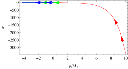
Hence, the second derivative of the scale factor , satisfies . Let us investigate whether the solution (18) is a stable attractor of the theory, and in Fig. 1 we have plotted the phase space behavior of the solution (18), by using the initial conditions (red line), (green line), (blue line), for . We need to note that for the numerical analysis we numerically solve the differential equation of Eq. (11), which we quote here for reading convenience,
| (22) |
which needs to be solved as a function of the cosmic time , and the function must be chosen as in Eq. (18). Since the differential equation is of first order, only one initial condition is needed, this is why we specified only the value of the scalar field at various cosmic time instances. So the numerical analysis will reveal if the solution (18) is a stable attractor of the one-dimensional dynamical system appearing in Eq. (22). Note that the explicit form of the function is not needed if we use the dynamical system (22). As it can be seen in Fig. 1, the phase space has an attractor which is reached by all the solutions as the field values decrease and also when the velocity of the field decreases too. Hence, the solution (18) is an attractor and this can also be verified analytically. By using Eq. (15), for the solution (18), we obtain,
| (23) |
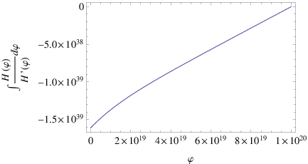
which is negative for the field values of interest. This can also be seen in Fig. (2), where we plotted the behavior of the perturbation exponent. Actually, the fact that the quantity appearing in Eq. (23) is negative is an important feature, as it was also pointed in Ref. [23], but also the important point is that the decay of the perturbation is exponential, as it can be seen from Eq. (15). Hence, we have verified that it is possible to realize the constant-roll to constant-roll transition, for the model (16), and the resulting solution (18) is a stable attractor of the theory.
Note that the numerical analysis we performed above aimed to investigate whether the solution , appearing in Eq. (18), is the stable attractor of the cosmological system, therefore the potential of Eq. (20) does not affect the phase space diagram, at least in our approach. As it can be seen in Fig. 1, there appear three curves which converge to the attractor point in the upper left. The difference between the three curves is that the red curve starts around , the green one starts at and also the blue at , as it is expected from the initial conditions. Recall that the dynamical system that corresponds to the phase space diagram is that of Eq. (22) appearing above, so the solution (18) is the attractor of the cosmological dynamical system (22). However, as we show later on, not all constant-roll models result to this behavior (see Fig. 10 in a later section).
Now let us investigate how the actual transition of one constant-roll era to the other is achieved, by distinguishing the two different eras, that is, we start with the era with and we shall try to see when this era ends, and also how it is possible for this era to end, so that the era with starts. It is conceivable that the continuous transition is guaranteed by the solution we found in Eq. (18), but if we distinguish the limiting cases of constant roll, then it is qualitatively more easy to understand some fundamental elements of the evolution, like for example the growth of perturbations. From a qualitative point of view, a constant-roll era can end if some sort of instability is caused in the cosmological system. In our case the transition is ensured by the form of the potential and of the function , and it is smooth, but it is worth discussing how this is possible by distinguishing the two eras.
So let us discuss the general case first, and we will perturb the limiting case,
| (24) |
Effectively we will examine the behavior of the perturbations around the limiting case where , with being a real number. As in Ref. [12], we define the following quantity,
| (25) |
and a study of the evolution of as a function of the scalar field may reveal when does the constant-roll era (24) ends. Notice that the following holds true,
| (26) |
which shows that the variable is strongly affected by the function . This means that when the function strongly varies as a function of , then the function also varies strongly. Actually, if we consider the linear perturbation of the solution , when the perturbations start to grow, which may occur after a particular value of the scalar field is reached, then the constant-roll era (24) practically ends. By differentiating the function with respect to , and by using the following relations,
| (27) |
after some algebra, it can be shown that the evolution of the quantity is determined by the following equation,
| (28) |
where is the first slow-roll index. Obviously, during the constant-roll era (24), the quantity is equal to one, so we linearly perturb the solution , and the perturbation satisfies the following differential equation,
| (29) |
The function captures the perturbations around the limiting constant-roll era (24), and in order to obtain the differential equations (28) and (29) we did not assume that the condition (24) holds true, this is just the limiting case scenario. The impact of the on the differential equations is imprinted in all cases on the variables and , and mainly on the latter, since this is the perturbation of the limiting case (24). In addition, it is the solution (18) which will determine the evolution of the perturbations and recall that the solution (18) was obtained by assuming that the function is not constant, but it is the one given in Eq. (16).
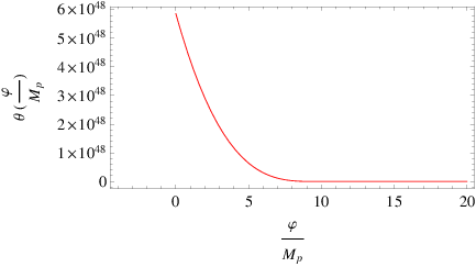
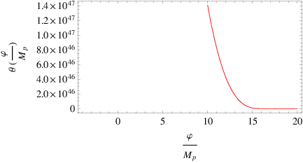
So by having the solution at hand, given in Eq. (18), we can investigate how the perturbations evolve as a function of the scalar field . Recall that the constant-roll limit of the function for large is , so in the large field limit we have . Therefore we shall perform a numerical analysis of the differential equation (29), with being as in Eq. (18). In Fig. 3 we present the results of our numerical analysis, for which we used various initial conditions. The resulting behavior of the perturbations strongly depend on the choice of the initial condition for , which must be chosen in such a way so that at large field values, we must have , in order to have . In Fig. 3 the plots are done in terms of , so the upper left and right plots correspond to , while the bottom plot corresponds to . It is conceivable that from a physical point of view, the perturbations should grow, since the function at still depends on the scalar field and decays to the final value as the field values decrease. So in principle small perturbations will destabilize the system, as it is expected. This behavior can be seen in all the plots of Fig. 3. The parameter changes its values quite slowly from until , so the perturbations, even small, destabilize the initial solution at , as it can be seen in the upper right plot, or even at , as it is shown in the bottom plot. Practically, the era lasts some -foldings, as it was expected, and the system makes a transition to intermediate states in the interval . Eventually for , the final constant-roll era with is reached.
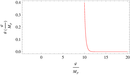
By following the same procedure, we can investigate what happens when the second constant-roll era is reached, which corresponds to . As it can be seen in Fig. 4, the numerical solution for the evolution of the perturbation seems quite stable, regardless what initial conditions we choose. For example, in the left plot of Fig. 4 we chose and for the right plot , and in both cases the perturbations remain quite small.
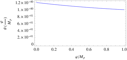
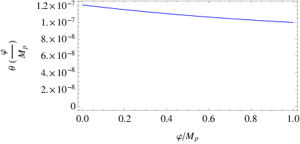
The behavior described by Fig. 4 was expected, since the function does not evolve after the constant-roll era is reached. This now raises the issue of graceful exit for this particular case, but this feature strongly depends on the choice of the parameters and , and also on the choice of the function which controls the smooth transition between the constant-roll eras. However, we did not aim to provide a completely viable model, but just to present how the transition mechanism behaves and how the actual transition can be achieved, mainly focusing on the qualitative features of it. Another question we would like to address in brief is the primordial curvature perturbations issue, and in the literature there appear already standards approaches devoted on the constant-roll era, see for example [12, 13]. Actually the results of [13] are identical to the ones obtained in [12], but the notation is different. In both cases an important assumption which we will also adopt is that the power spectrum must not be calculated at the horizon crossing, but at the time of consideration, possibly when inflation comes to an end. Also an important assumption is that the subhorizon state is described by a Bunch-Davies vacuum state, but this is not necessarily true in the case at hand, however we do not discuss this issue further at this point.
Coming back to the power spectrum, we quote here the result of [12, 13] for the power spectrum, which is,
| (30) |
and the tilt of the power spectrum is,
| (31) |
so the resulting spectral index is,
| (32) |
However, for the case the power spectrum is not scale invariant, as it can be easily seen. Also the resulting spectral index which is is not compatible with the observational data coming from the Planck collaboration [1]. Of course our aim was not to provide a completely viable model, but to show how the transition mechanism between constant-roll eras works. If the function is chosen to have better behavior than the particular choice we made, then perhaps a more refined phenomenology could in principle be produced. Such an example is given in the next section.
IV Model II
Let us discuss the qualitative features of another model, in which case the function of Eq. (10) has the following form,
| (33) |
which is a monotonic function of . The parameter is chosen as in Eq. (17), while and are positive dimensionless real numbers, which we specify later on in this section.
In the limit , the function behaves as , so this describes a constant-roll era, and in the limit the function behaves as . A phenomenologically interesting scenario occurs for the following choice of the parameters,
| (34) |
in which case in the large field limit, we have , while in the small field limit we have . By solving the differential equation (12), in this case we get,
| (35) |
where is an integration constant. The corresponding scalar potential can be found by using (13),
| (36) | ||||
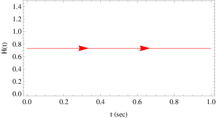
The behavior of the Hubble rate as a function of the cosmic time can only be found numerically, by finding the solution , so by solving numerically the differential equation (11) for , in Fig. 5 we can see that for a quite large era the Hubble rate is almost constant, so it approaches a de Sitter solution.
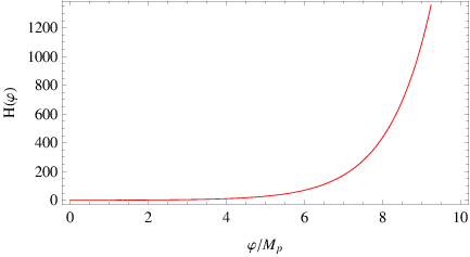
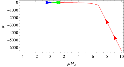
The solution (35) is a stable attractor as our numerical analysis shows in Fig. 6, where we used the values for the parameters as in Eq. (34), and also the initial conditions, (red line), (green line), (blue line).
What we are mainly interested for in this section is the behavior of the linear perturbations , the evolution of which is described by the differential equation (29).
Without getting into many details, the first constant-roll era, which corresponds to , is quite unstable as it was expected, since the function for these field values, is not slowly varying. However as the field value decreases, the function approaches its limiting value , which is quite stable. Indeed this can be verified for various initial conditions of , and the resulting evolution of perturbations is zero for .
In effect, this constant-roll era is also haunted by the graceful exit issue, however, if the primordial perturbations are generated during this era, which can be insured if the preceding constant-roll era lasts only a few -folds, then, the resulting power spectrum is [12, 13],
| (37) |
so the resulting spectral index is,
| (38) |
For the values of the parameters chosen as in Eq. (34), the resulting spectral index is , so it is in agreement with the Planck data [1]. Therefore this particular model shows that a viable phenomenology may be provided by constant-roll to constant-roll transitions. However, this model cannot be considered as being a completely viable, since there are various important theoretical issues that need to be amended, like the exit issue, the initial state issue and the horizon crossing issue. The complete study of these issues, exceeds the introductory aim of this work.
In principle, the constant-roll to constant-roll transitions may have an oscillatory behavior between constant-roll era. In the next section we briefly discuss a toy model that exhibits this kind of behavior.
V A Model Describing Oscillations Between Constant-Roll Eras
Consider the following model for the function ,
| (39) |
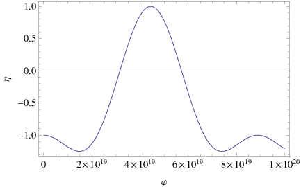
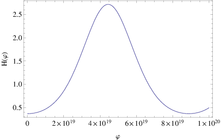
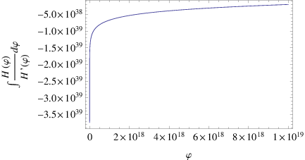
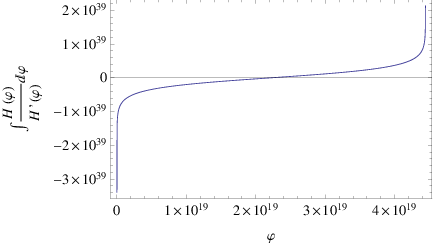
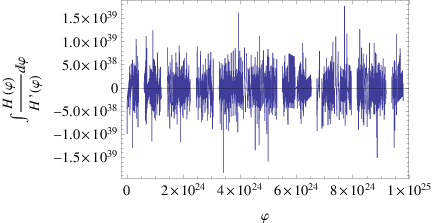
where is given in Eq. (17). It is obvious from the form of the function (39), that it can take bounded values, due to the presence of the trigonometric functions, and also it can be equal to zero. Hence, the cosmological system experiences transitions between the slow-roll and constant-roll era, and also from constant-roll to constant-roll. In order to have a concrete idea of the behavior of , in Fig. 7 we plot the -dependence of for field values in the interval . As it can be seen, the second slow-roll index oscillates between constant and slow-roll eras, if of course the resulting Hubble rate is an inflationary attractor. This is what we will investigate now.
The solution of the differential equation (12), for the function chosen in Eq. (39), is given below,
| (40) |
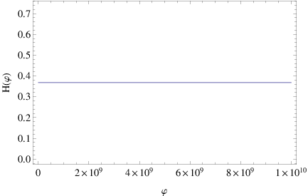
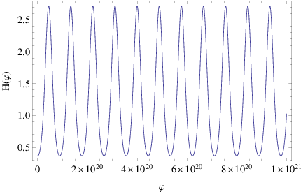
and in Fig. 8 we plot the -dependence of the Hubble rate given in Eq. (40). As it can be seen, the oscillatory behavior occurs in the Hubble rate too, and the Hubble rate goes from a de Sitter vacuum to a de Sitter vacuum, which correspond to the minima and maxima of the function .
By substituting Eq. (40) in Eq. (13) we can find the potential which is,
| (41) |
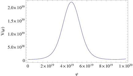
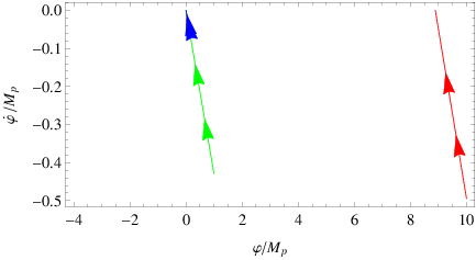
In Fig. 9 we plot the potential (41) for . We need to investigate the stability properties of the solution appearing in Eq. (40), and in Fig. 10 we present the results of our numerical analysis. We use three different initial conditions, namely, (red line), (green line), (blue line). As it can be seen, for the first initial condition, the attractor is different in comparison to the other two initial conditions. Oddly, after , the system develops peculiar properties, and becomes very unstable. This can also be seen in Fig. 11, where we plot the behavior of the linear perturbations (15), and as it can be seen, after , the perturbations grow, and after , they develop a quite intense oscillatory behavior. Therefore, the model (39) after becomes unstable, however for smaller field values, the solution (40) seems to be the attractor of the cosmological system. Hence, the model (39), has an odd behavior for large field values, however for values , it has interesting phenomenology, since it allows oscillations between different roll eras. Particularly it allows transitions between constant-roll eras and slow-roll eras. A refined model of this sort could potentially have an interesting phenomenology, but we defer this study to a future work.
VI Concluding Remarks
In this paper we presented various models which allow transitions between constant-roll eras. This was achieved by assuming that the second slow-roll index is equal to a function of the scalar field . Then, by appropriately choosing the function, it is possible to produce transitions between constant-roll eras, and also it is possible to provide more involved transition scenarios. We mainly focused on the stability behavior of the solutions and we did not study in detail the phenomenological implications of the models studied. As we demonstrated, one of the models we studied, has very good stability properties and also the solution is the attractor of the cosmological equations. Another model we studied, which produces oscillating transitions between constant-roll eras, is stable for a , so it has limited interest in comparison to the other two models we presented.
In the class of exponential models we studied, we demonstrated that the constant-roll eras are realized in the large and small field values limits. As we demonstrated, the first constant-roll era is unstable and the final constant-roll era is stable towards linear perturbations of the constant-roll condition. This raises the question with regards to the graceful exit, and if it is possible for the system to finally exit from inflation. The lack of analyticity in some cases makes it difficult to quantify the slow-roll indices in terms of the -foldings number, but in principle the most interesting scenario is to combine the constant-roll era(s) with a slow-roll era, in the spirit of Ref. [20], however the system should result to a slow-roll era. In this way the slow-roll era could end in the usual way it does in single scalar theories, when the slow-roll indices become of order one. This feature is also an indication for the graceful exit from inflation. Another issue is the calculation of the power spectrum during the constant-roll eras, in which we used standard approaches. However, an issue regarding the calculation is the horizon crossing, since the power spectrum is not calculated at the horizon crossing, so this is different in spirit in comparison to the ordinary slow-roll case. As we showed by using the same approach as in the related literature, the resulting power spectrum can be nearly scale invariant. In conclusion, the virtue of having two constant-roll eras is that the theory is more free from unnecessary fine tunings, however the issue of the graceful exit persists. We believe that the best proposal in this context is to have a constant-roll era that ends up to a slow-roll era with the mechanism we presented in this work. In this way, the theory develops non-Gaussianities, which can be potentially measured by future observations, but also the same theory can yield observational indices corresponding to the slow-roll era. Accordingly, the exit from inflation can come as an outcome of the ending of the slow-roll era.
In a future work we shall address the phenomenological implications of the models presented in this paper, mainly focusing on the non-Gaussianities that can be produced during the constant-roll eras. Of course it is conceivable that the models we presented cannot be considered viable unless these produce results compatible with the observational data, and also these models must solve simultaneously the graceful exit issue and the non-Gaussianities issue. However, our aim was not to provide viable models to all aspects, but to present models that allow transitions between constant-roll eras. Finding a viable model with these features is of course the goal, but a more refined choice for the function is required, and also the combination of an initial constant-roll era that ends up to a slow-roll era seems the most favorable scenario.
Acknowledgments
This work is supported by MINECO (Spain), project FIS2013-44881, FIS2016-76363-P and by CSIC I-LINK1019 Project (S.D.O) and by Min. of Education and Science of Russia (S.D.O and V.K.O).
References
- [1] P. A. R. Ade et al. [Planck Collaboration], Astron. Astrophys. 594 (2016) A20 [arXiv:1502.02114 [astro-ph.CO]].
- [2] A. D. Linde, Lect. Notes Phys. 738 (2008) 1 [arXiv:0705.0164 [hep-th]].
- [3] D. S. Gorbunov and V. A. Rubakov, “Introduction to the theory of the early universe: Cosmological perturbations and inflationary theory,” Hackensack, USA: World Scientific (2011) 489 p;
- [4] D. H. Lyth and A. Riotto, Phys. Rept. 314 (1999) 1 [hep-ph/9807278].
- [5] K. Bamba and S. D. Odintsov, Symmetry 7 (2015) 1, 220 [arXiv:1503.00442 [hep-th]]
- [6] X. Chen, Adv. Astron. 2010 (2010) 638979 doi:10.1155/2010/638979 [arXiv:1002.1416 [astro-ph.CO]].
- [7] S. Inoue and J. Yokoyama, Phys. Lett. B 524 (2002) 15 doi:10.1016/S0370-2693(01)01369-7 [hep-ph/0104083].
- [8] N. C. Tsamis and R. P. Woodard, Phys. Rev. D 69 (2004) 084005 doi:10.1103/PhysRevD.69.084005 [astro-ph/0307463].
- [9] W. H. Kinney, Phys. Rev. D 72 (2005) 023515 doi:10.1103/PhysRevD.72.023515 [gr-qc/0503017].
- [10] K. Tzirakis and W. H. Kinney, Phys. Rev. D 75 (2007) 123510 doi:10.1103/PhysRevD.75.123510 [astro-ph/0701432].
- [11] M. H. Namjoo, H. Firouzjahi and M. Sasaki, Europhys. Lett. 101 (2013) 39001 doi:10.1209/0295-5075/101/39001 [arXiv:1210.3692 [astro-ph.CO]].
- [12] J. Martin, H. Motohashi and T. Suyama, Phys. Rev. D 87 (2013) no.2, 023514 doi:10.1103/PhysRevD.87.023514 [arXiv:1211.0083 [astro-ph.CO]].
- [13] H. Motohashi, A. A. Starobinsky and J. Yokoyama, JCAP 1509 (2015) no.09, 018 doi:10.1088/1475-7516/2015/09/018 [arXiv:1411.5021 [astro-ph.CO]].
- [14] Y. F. Cai, J. O. Gong, D. G. Wang and Z. Wang, JCAP 1610 (2016) no.10, 017 doi:10.1088/1475-7516/2016/10/017 [arXiv:1607.07872 [astro-ph.CO]].
- [15] H. Motohashi and A. A. Starobinsky, arXiv:1702.05847 [astro-ph.CO].
- [16] S. Hirano, T. Kobayashi and S. Yokoyama, Phys. Rev. D 94 (2016) no.10, 103515 doi:10.1103/PhysRevD.94.103515 [arXiv:1604.00141 [astro-ph.CO]].
- [17] L. Anguelova, Nucl. Phys. B 911 (2016) 480 doi:10.1016/j.nuclphysb.2016.08.020 [arXiv:1512.08556 [hep-th]].
- [18] J. L. Cook and L. M. Krauss, JCAP 1603 (2016) no.03, 028 doi:10.1088/1475-7516/2016/03/028 [arXiv:1508.03647 [astro-ph.CO]].
- [19] K. S. Kumar, J. Marto, P. Vargas Moniz and S. Das, JCAP 1604 (2016) no.04, 005 doi:10.1088/1475-7516/2016/04/005 [arXiv:1506.05366 [gr-qc]].
- [20] S. D. Odintsov and V. K. Oikonomou, arXiv:1703.02853 [gr-qc].
- [21] J. Lin, Q. Gao and Y. Gong, Mon. Not. Roy. Astron. Soc. 459 (2016) no.4, 4029 doi:10.1093/mnras/stw915 [arXiv:1508.07145 [gr-qc]].
- [22] Q. Gao and Y. Gong, arXiv:1703.02220 [gr-qc].
- [23] A. R. Liddle, P. Parsons and J. D. Barrow, Phys. Rev. D 50 (1994) 7222 doi:10.1103/PhysRevD.50.7222 [astro-ph/9408015].
- [24] J. E. Lidsey, Phys. Lett. B 273 (1991) 42. doi:10.1016/0370-2693(91)90550-A
- [25] J. E. Lidsey, Class. Quant. Grav. 8 (1991) 923. doi:10.1088/0264-9381/8/5/016