Stable Throughput and Delay Analysis of a Random Access Network With Queue-Aware Transmission
Abstract
In this work we consider a two-user and a three-user slotted ALOHA network with multi-packet reception (MPR) capabilities. The nodes can adapt their transmission probabilities and their transmission parameters based on the status of the other nodes. Each user has external bursty arrivals that are stored in their infinite capacity queues. For the two- and the three-user cases we obtain the stability region of the system. For the two-user case we provide the conditions where the stability region is a convex set. We perform a detailed mathematical analysis in order to study the queueing delay by formulating two boundary value problems (a Dirichlet and a Riemann-Hilbert boundary value problem), the solution of which provides the generating function of the joint stationary probability distribution of the queue size at user nodes. Furthermore, for the two-user symmetric case with MPR we obtain a lower and an upper bound for the average delay without explicitly computing the generating function for the stationary joint queue length distribution. The bounds as it is seen in the numerical results appear to be tight. Explicit expressions for the average delay are obtained for the symmetrical model with capture effect which is a subclass of MPR models. We also provide the optimal transmission probability in closed form expression that minimizes the average delay in the symmetric capture case. Finally, we evaluate numerically the presented theoretical results.
Index Terms:
Boundary Value Problem, Stable Throughput Region, Delay Analysis, Random AccessI Introduction
The ALOHA protocol since its creation [1] has gained popularity in multiple access communication systems for its simple nature and the fact that it does not require centralized controllers. This simple scheme attempts transmission randomly, independently, distributively, and based on a simple ACK/NACK feedback from the receiver.
Random access recently re-gained interest due to the increase in the number of communicating devices in 5G networks, more specifically, because of the need of massive uncoordinated access in large networks [2, 3]. Random access and alternatives and their effect on the operation of LTE and LTE-A are presented in [2, 4, 5]. Recently, the effect of random access in physical layer and in other topics has been studied [6, 7, 8, 9] and the research in this area is in progress. Random access remains an active research area where a lot of fundamental questions remain open even for very simple networks [10, 11].
When the traffic in a network is bursty, a relevant performance measure is the stable throughput or stability region. The exact characterization of the stability region is known to be a difficult problem due to the interaction among the queues. Except the throughput, delay is another important metric. Recently there is a rapid growth on supporting real-time applications thus, there is a need to provide delay-based guarantees [3, 12]. Thus, the characterization of the delay is of major importance. However, the exact characterization of delay even in small networks with random access is rather difficult and remains unexplored in most of the cases.
In this work, we consider a two-user and a three-user slotted ALOHA network with multi-packet reception capabilities. Furthermore, the nodes can adapt their transmission probabilities and their transmission parameters based on the status of the other node. We analyze the stable throughput region and study the queueing delay by utilizing the theory of boundary value problems.
I-A Related Work
In the literature so far there is a vast number of papers that are considering the stable throughput and delay in random access and variations of random access schemes.
The derivation of the stability region of random access systems for bursty sources is known to be a difficult problem above three sources. This is because each source transmits and interferes with the others only when its queue is non-empty. Such queues where the service process of one depends on the status of the others are said to be coupled or interacting. Thus, the individual departure rates of the queues cannot be computed separately without knowing the stationary distribution of the joint queue length process [13]. This is the reason why the vast majority of previous works has focused on small-sized networks and only bounds or approximations are known for the networks with larger number of sources [14, 13, 15, 16, 17, 7]. In [18], an approximation of the stability region was obtained based on the mean-field theory for network of nodes having identical arrival rates and transmission probabilities were performed. The work in [19] investigates the stable throughput region of a random access network where the transmitters and receivers are distributed by a static Poisson bipolar process.
Delay analysis of random access networks was studied in [17, 20, 21]. More specifically, in [17, 7] a two-user network with MPR capabilities was considered and expressions for the average delay were obtained for the symmetric case. The papers [20, 21] considered collision channel model. In [22] the delay performance of slotted ALOHA in a Poisson network was studied. Delay analysis of random access networks based on fluid models can be found in [23] and in [24]. The works [25] and [26] utilized techniques from statistical mechanics for throughput and delay analysis. The authors in [27] proposed a service-martingale concept that enables the queueing analysis of a bursty source sharing a MAC channel.
Below we present a recent set of papers that consider throughput and/or delay characterization of general random access networks. The work in [28] studied the impact of a full duplex relay in terms of throughput and delay in a multi-user network, where the users were assumed to have saturated traffic. The delay of a random access scheme in the Internet of Things concept was studied in [29]. In [30] throughput with delay constraints was studied in a shared access cognitive network. The delay characterization of larger networks was considered in [31, 32]. In [33] the delay and the packet loss rate of a frame asynchronous coded slotted ALOHA system for an uncoordinated multiple access were also studied.
I-B Contribution
Our contribution in this work can be summarized as follows. We consider the case of the two and three-user wireless network with a common destination. The nodes/sources access the medium in a random access manner and time is assumed to be slotted. Each user has external bursty arrivals that are stored in their infinite capacity queues. We consider multi packet reception (MPR) capabilities at the destination node.
The nodes are accessing the wireless channel randomly and they adapt their transmission probabilities based on the status of the queue of the other nodes. More precisely, a node adapt its transmission characteristics based on the status of the other node in order to exploits its idle slots and to increase the chances of a successful packet transmission. To the best of our knowledge this variation of random access has not been reported in the literature. The contribution of this work has two main parts focused on the stable throughput region and the detailed analysis of the queueing delay at users nodes.
I-B1 Stable Throughput Region Analysis
The first part is related to the study of stable throughput.
- •
More specifically, we obtain the stability conditions for the case of two and three users. To the best of our knowledge, there is no other work in the related literature that deals with the stability region of a random access system with adaptive transmission control. Furthermore, we obtain the conditions where the stability region is a convex set. Convexity is an important property since it corresponds to the case when parallel concurrent transmissions are preferable to a time-sharing scheme.
- •
We would like also to emphasize that the exact stability region for the case of three nodes with MPR even in the simple random access (without transmission control) case is not known in the literature, except for the case of a collision channel model [34].
The main difficulty for characterizing the stability region lies on the interaction of the queues. The interaction of the queues arise when the service rate of a queue depends on the state of the other. A tool to bypass this difficulty is the stochastic dominance technique introduced in [13]. However, the three-user network is more elaborated and the stability region cannot be derived that easily. As mentioned also earlier, in the literature the three-user scenario has studied only for the collision channel model.
I-B2 Delay Analysis
The second part of the contribution of this work is the delay analysis.
- •
Based on a relation among the values of the transmission probabilities we distinguish the analysis in two cases, which are different in the modeling and the technical point of view. In particular, the analysis leads to the formulation of two boundary value problems (e.g., [35, 36, 37, 38, 39]), the solution of which will provide the joint probability distribution of the queue size for the two-user case with MPR. The analysis is rather complicated and novel.
- •
Furthermore, for the two-user symmetric case with MPR we obtain a lower and an upper bound for the average delay without explicitly computing the generating function for the stationary joint queue length distribution.
- •
The bounds as it is seen in the numerical results appear to be tight. Explicit expressions for the average delay are obtained for the model with capture effect, i.e., a subclass of MPR models.
- •
We also provide the optimal transmission probability in closed form expression that minimizes the average delay in the symmetric capture case.
Concluding, the analytical results in this work, to the best of our knowledge, have not been reported in the literature.
The rest of the paper is organized as follows. In Section II we present the system model by providing the details of the proposed protocol and the underlying physical layer details on the channel model. In Section III we provide the stability region for the two-user case for the proposed random access scheme. In Section IV we derive the fundamental functional equation and obtain some important results for the following analysis. Section V is devoted to the formulation of two boundary value problems, the solution of which provides the generating function of the joint stationary queue length distribution of user nodes. The expected number of packets and the average delay expressions are also obtained. In Section VI, we provide an alternative approach to obtain the stability conditions and we also obtain the exact expressions for the stability region for the case of three users. In Section VII, we obtain explicit expressions for the average delay at each user for the symmetrical system. Finally, numerical examples that provide insights in the system performance are given in Section VIII.
II System Model
II-A Network Model
We consider a slotted random access system consisting of users communicating with a common receiver. Each user has an infinite capacity buffer, in which stores arriving and backlogged packets. Packets have equal length and the time is divided into slots corresponding to the transmission time of a packet. Let be a sequence of independent and identically distributed random variables where is the number of packets arriving in user node , , in the time interval , with , . Denote also by , , , , the generating function of the joint distribution of the number of arrivals in any slot.
At the beginning of each slot, there is a probability for the node , , to transmit a packet to the receiver. More than one concurrent transmission can occur without having a collision.
Due to the interference and the complex interdependence among the nodes we consider the following queue-aware transmission policy: If both nodes are non empty, node , transmits a packet with probability independently, where is the probability that node does not make a transmission in a slot when its queue is not empty. If node 1 (resp. 2) is the only non-empty, it transmits a packet with probability , where is the probability that node does not make a transmission in the given slot. 11 1 We consider the general case for instead of assuming directly . This can handle cases where the node cannot transmit with probability one even if the other node is silent. This scenario for example can occur when the nodes are subject to energy limitations. It is outside of the scope of this work to consider specific reasons when this case can appear but we want to keep the proposed analysis general. Note that in our case, a node is aware about the state of its neighbor. 22 2 In a shared access network, it is practical to assume some minimum exchanging information of one bit in this case.
II-B Physical Layer Model
The MPR (Multi-Packet Reception) channel model used in this paper is a generalized form of the packet erasure model. In the wireless environment, a packet can be decoded correctly by the receiver if the received SINR exceeds a certain threshold. More precisely, suppose that we are given a set of nodes transmitting in the same time slot. Let be the signal power received from node at node (when transmits), and let be the SINR received by node j, i.e., , where denotes the receiver noise power at . We assume that a packet transmitted by is successfully received by if and only if , where is the SINR threshold. The wireless channel is subject to fading; let be the transmitting power at node and be the distance between and . The power received by when transmits is where is a random variable representing channel fading. We assume that the fading model is slow, flat fading, constant during a time slot and independently varying from time slot to time slot. Under Rayleigh fading, it is known [40] that is exponentially distributed. The received power factor where is the path loss exponent with typical values between and . In this study we consider one destination which is common for both nodes, thus denotes the common destination here and we can also write . The success probability of link when the transmitting nodes are in is given by [40]
| (1) |
where is the parameter of the Rayleigh random variable for fading. According to (1) we denote to be the success probability of node when the transmitting nodes are and , . More precisely: the strongest user can be successfully received even in the presence of simultaneous transmissions (i.e., collision), if the difference in power is large enough [41] (provided that ). If both nodes transmit, but their are below the threshold , their transmission is unsuccessful.
Next, we will define for convenience some conditional probabilities on top of the expression given in (1).33 3 A similar approach can be found in [17, 7]. We define the probability that when both nodes and are transmitting only the transmission from node is successful. Then . Similarly we can define . The is the probability that both packets transmitted by nodes and are transmitted successfully, then . Thus, , then we have that .
The is the probability where both packets fail to reach the destination when both nodes and are transmitting, then . Note that is the success probability of node when only -th node transmits but the other one is active (i.e., there are packets stored in its buffer), we denote with the outage probability respectively. Furthermore, we assume that a node adjusts its transmission parameters such as the transmission power when the other node has an empty queue (i.e is inactive). Thus, the success (resp. outage) probability of node when the other node is inactive is denoted by (resp. ). By allowing this we can consider a simple power control policy where a node can adapt its transmission power when the other node is empty, in order to increase the success probability thus, is reasonable to assume that .
In the case of an unsuccessful transmission the packet has to be re-transmitted later. We assume that the receiver gives an instantaneous (error-free) feedback (ACK) of all the packets that were successful in a slot at the end of the slot to all the nodes. The nodes remove the successfully transmitted packets from their buffers. The packets that were not successfully transmitted are retained.
Now we can write the expressions for the average service rates and seen at node and respectively. The expression for is given below and similarly we can obtain . Denote by the length of queue at the beginning of time slot . Then,
| (2) |
where , . We can easily see from (2) that the service rate of one queue depends on the status of the other queue. Thus, the queues are coupled. In Section III we bypass this difficulty by applying the stochastic dominance technique to obtain the exact stability region. Regarding the delay analysis we need a different treatment, based on the powerful and technical theory on boundary value problems; see Section V.
Based on the definition in [34], a user’s node is said to be stable if and . Loynes’ theorem [42] states that if the arrival and service processes of a queue are strictly jointly stationary and the average arrival rate is less than the average service rate, then the queue is stable. If the average arrival rate is greater than the average service rate, then the queue is unstable and the value of approaches infinity almost surely. The stability region of the system is defined as the set of arrival rate vectors , for which the queues in the system are stable.
III Stability Region for users
In this section, we derive the stability region, i.e., the region of values for , , for which our system is stable. The following theorem provides the stability conditions for the two-user random access network.
Theorem III.1.
The stability region for a fixed transmission probability vector is given by where
| (3) | |||
| (4) |
where for , , , , .
Proof.
To determine the stability region of our system (depicted in Fig. 1) we apply the stochastic dominance technique [13], i.e. we construct hypothetical dominant systems, in which the source transmits dummy packets for the packet queue that is empty, while for the non-empty queue it transmits according to its traffic. Under this approach, we consider the , and -dominant systems. In the dominant system, whenever the queue of user , empties, it continues transmitting a dummy packet.
Thus, in , node never empties, and hence, node sees a constant service rate, while the service rate of node depends on the state of node , i.e., empty or not. We proceed with queue at node . The service rate of the first node is given by (2). The service rate of the second user is given by
| (5) |
By applying Loyne’s criterion, the second node is stable if and only if the average arrival rate is less that the average service rate, . We can obtain the probability that the second node is empty and is given by . After replacing into (2), and applying Loynes criterion we can obtain the stability condition for the first node. Then, we have the stability region given by (3). Note that the expression in (3) is given in a more compact form that it will be useful in the next sections. Similarly, we can obtain the stability region for the second dominant system , the proof is omitted due to space limitations. For a detailed treatment of dominant systems please refer to [13].
An important observation made in [13] is that the stability conditions obtained by the stochastic dominance technique are not only sufficient but also necessary for the stability of the original system. The indistinguishability argument [13] applies here as well. Based on the construction of the dominant system, we can see that the queue sizes in the dominant system are always greater than those in the original system, provided they are both initialized to the same value and the arrivals are identical in both systems. Therefore, given , if for some , the queue at the first user is stable in the dominant system, then the corresponding queue in the original system must be stable. Conversely, if for some in the dominant system, the queue at the first node saturates, then it will not transmit dummy packets, and as long as the first user has a packet to transmit, the behavior of the dominant system is identical to that of the original system since dummy packet transmissions are eliminated as we approach the stability boundary. Therefore, the original and the dominant system are indistinguishable at the boundary points. ∎
Remark 1.
The stability region is a convex polyhedron when the following condition holds . When equality holds in the previous condition as depicted also in Fig. 1, the region is a triangle and coincides with the case of time-sharing. Convexity is an important property since it corresponds to the case when parallel concurrent transmissions are preferable to a time-sharing scheme. Additionally, convexity of the stability region implies that if two rate pairs are stable, then any rate pair lying on the line segment joining those two rate pairs is also stable.
Remark 2.
The condition is the generalized version of the condition that characterizes the MPR capability in the system which was first appeared in [17].

IV Preparatory Analysis & Results
In this section we provide the first part of the analysis that is needed to obtain the expressions for the delay analysis. More explicitly, we derive the fundamental functional equation and we obtain some important results that we will use in the analysis of Section V.
Let be the number of packets in user node at the beginning of the th slot. Then, is a two-dimensional Markov chain with state space is describing our system model. The queues of both users evolve as , where is the number of departures from user queue at time slot . Then, the queue evolution equation implies
| (6) |
where denotes the indicator function of the event . Assuming that the system is stable, let . Using (6) after some algebra we obtain the following functional equation,
| (7) |
where
In the following, we will solve (7) by assuming geometrically distributed arrival processes at both stations, which are assumed to be independent. More precisely, we assume , , .
Remark 3.
Without loss of generality, it is realistic to assume that , . Indeed, is the difference of the successful transmission probability of node , when both nodes are active (i.e., both nodes have packets to send) minus the successful transmission probability of node when the other node is inactive (i.e., only node has packets to send). Clearly, in the later case due to the lack of interference and since node senses the other node inactive will transmit with a higher probability in order to exploit the idle slot of the other node. Definitely, in such a case .44 4 The particular case where is omitted since there is no coupling between the queues and the analysis becomes trivial. Therefore from hereon we assume that , .
Some interesting relations can be obtained directly from the functional equation (7). Taking , dividing by and taking in (7) and vice versa yield the following “conservation of flow” relations:
| (8) |
| (9) |
where , .
In the following, the analysis is distinguished in two cases:
- 1.
- 2.
We now focus on the derivation of some preparatory results in view of the resolution of functional equation (7). More precisely, we focus on the analysis of the kernel equation .
IV-A Analysis of the kernel
In the following we consider the kernel equation and provide some important properties. We focus on a subclass of MPR channels, the so called “capture” channels, i.e., (at most one user has a successful packet transmission even if many users transmit in that slot [43, 44]). Note that, , where, , , , , . The roots of are , , where , .
Lemma IV.1.
For , , the kernel equation has exactly one root such that . For , . Similarly, we can prove that has exactly one root , such that , for .
Proof.
It is easily seen that , where , where for , , is a generating function of a proper probability distribution. Now, for , and it is clear that . Thus, from Rouché’s theorem, has exactly one zero inside the unit circle. Therefore, has exactly one root , such that . For , implies . Therefore, for , and since , the only root of for , is . ∎
Lemma IV.2.
The algebraic function , defined by , has four real branch points . Moreover, , and , . Similarly, , defined by , has four real branch points . Moreover, , and , .
Proof.
The proof is based on simple algebraic arguments and further details are omitted due to space limitations. ∎
To ensure the continuity of the function two valued function (resp. ) we consider the following cut planes: , , where , the complex planes of , , respectively. In (resp. ), denote by (resp. ) the zero of (resp. ) with the smallest modulus, and (resp. ) the other one.
Define the image contours, , , where stands for the contour traversed from to along the upper edge of the slit and then back to along the lower edge of the slit. The following lemma shows that the mappings , , for , respectively, give rise to the smooth and closed contours , respectively.
Lemma IV.3.
- 1.
For , the algebraic function lies on a closed contour , which is symmetric with respect to the real line and defined by , , and , where, , . Set , the extreme right and left point of , respectively.
- 2.
For , the algebraic function lies on a closed contour , which is symmetric with respect to the real line and defined by , , where , . Set , the extreme right and left point of , respectively.
Proof.
We will prove the part related to . Similarly, we can also prove part 2. For , is negative, so and are complex conjugates. It also follows that
| (11) |
Therefore, . Clearly, is an increasing function for and thus, . Finally, is derived by solving (11) for with , and taking the solution such that . ∎
V The boundary value problems
As indicated in the previous section, based on a relation between the transmission probabilities of the users, we distinguish the analysis in two cases, which differ both from the modeling and the technical point of view. In this section we consider the case where .
V-A A Dirichlet boundary value problem
Assume now that . Then, . Therefore, for ,
| (12) |
For both , are analytic and the right-hand side can be analytically continued up to the slit , or equivalently,
| (13) |
Then, multiplying both sides of (13) by the imaginary complex number , and noticing that is real for , since , we have
| (14) |
Clearly, some analytic continuation considerations must be made in order to have everything well defined. Thus, we have to check for poles of in , where be the interior domain bounded by , and , , . These poles, if exist, they coincide with the zeros of in (see Appendix). In order to solve (14), we must first conformally transform the problem from to the unit circle . Let the conformal mapping, , and its inverse .
Then, we have the following problem: Find a function regular for , and continuous for such that, , . To proceed, we need a representation of in polar coordinates, i.e., This procedure is described in detail in [35]. In the following we summarize the basic steps: Since , for each , a relation between its absolute value and its real part is given by (see Lemma IV.3). Given the angle of some point on , the real part of this point, say , is the solution of , Since is a smooth, egg-shaped contour, the solution is unique. Clearly, , and the parametrization of in polar coordinates is fully specified. Then, the mapping from to , where and , satisfying and is uniquely determined by (see [35], Section I.4.4),
| (15) |
i.e., is uniquely determined as the solution of a Theodorsen integral equation with . Due to the correspondence-boundaries theorem, is continuous in .
In the case that has no poles in , the solution of the problem defined in (14) is:
| (16) |
where , is a constant that can be defined by setting in (16) and using the fact that , . In the case that has a pole, it will be (see Appendix), and we still have a Dirichlet problem for the function .
Following the discussion above, . Setting , , we obtain after some algebra,
which is an odd function of . Thus, . Substituting back in (16) we deduce after simple calculations
| (17) |
A detailed numerical approach in order to obtain the inverse mapping is presented in the seminal book [35]. Similarly, we can determine by solving another Dirichlet boundary value problem on the closed contour . Then, using the fundamental functional equation (7) we uniquely obtain .
V-B A homogeneous Riemann-Hilbert boundary value problem
We now assume that . In such a case we consider the following transformation:
Then, for , (7) yields . For both , are analytic and the right-hand side can be analytically continued up to the slit , or equivalently for ,
| (18) |
Clearly, is holomorphic in , continuous in . However, might has poles, based on the values of the system parameters in . These poles (if exist) coincide with the zeros of in ; see Appendix. For , let and realize that so that (note that following [39] , ). Taking into account the possible poles of , and noticing that is real for , since , we have
| (19) |
where , whether is zero or not of in . Thus, is regular for , continuous for , and is a non-vanishing function on . We must first conformally transform the problem (19) from to the unit circle . Let the conformal mapping , and its inverse given by .
Then, the Riemann-Hilbert problem formulated in (19) is reduced to the following: Find a function , regular in , continuous in such that, .
A crucial step in the solution of the problem defined by (19) is the determination of the index , where , denotes the variation of the argument of the function as moves along the closed contour in the positive direction, provided that , . Following the lines in [36] we have,
Lemma V.1.
- 1.
If , then is equivalent to
- 2.
If , is equivalent to .
Therefore, under stability conditions (see Lemma III.1) the problem defined in (19) has a unique solution given by,
| (20) |
where is a constant and , , . Setting in (20) we derive a relation between and . Then, for , and using the first in (10) we can obtain and . Substituting back in (20) will give
| (21) |
Similarly, we can determine by solving another Dirichlet boundary value problem on the closed contour . Then, using the fundamental functional equation (7) we uniquely obtain .
V-C Expected Number of Packets and Average Delay
In the following we derive formulas for the expected number of packets and the average delay at each user node in steady state, say and , respectively. Denote by , the derivatives of with respect to and respectively. Then, , and using Little’s law , . Using the functional equation (7) and (8), (9) we derive
| (22) |
We only focus on , (similarly we can obtain , ). Note that can be obtained using (21) or (17) depending on the value of . For the case , using (21),
| (23) |
Substituting (23) in (22) we obtain , and dividing with , the average delay . Note that the calculation of (15) requires the evaluation of integrals (15), and , . For an efficient numerical procedure see [35], Chapter IV.1.
VI Stability conditions: Extension to the case of users
In the following, we provide sufficient and necessary conditions for the the case of users based on [15]. In particular we generalize the results in [15], by including the effect of capture channel as well as the queue-aware transmission policy. We accomplish this by means of a technique based on three simple observations: isolating a single queue from the system, applying Loynes’ stability criteria for such an isolated queue, and using stochastic dominance and mathematical induction to verify the required stationarity assumptions in the Loynes’ criterion. Below, we present an informal overview of the approach. First of all, we construct a modified system as follows. Let be a partition of such that users in operate exactly as in the original model, while users in are able to send packets even if their buffers are empty (e.g., dummy packets). Note that a system consisting of users in forms a smaller copy of the original system with slightly new probabilities of transmissions. Furthermore, it is easy to see that the modified system, stochastically dominates the queue lengths process in the original system (see [34, 15]). Therefore, proving stability of such a dominant system - that is, the one under the partition - suffices for stability of the original system. To accomplish this, we prove stability conditions for users in by mathematical induction. Finally, the stability region for the original system is a union of stability regions obtained for every partition ; see Theorem in [15]. However, as proved in [15], only partitions , where contribute to the final stability region.
VI-A An alternative approach for the case of users
We will present an alternative approach for the derivation of the stability region for the case of users in order to assist the analysis for the case of users. For such a case we consider the partitions , , where and , and let be stability region for the partition , . We will discuss the construction of in detail, then similarly the rest can be obtained. Denote by the probability of a successful transmission from user in the dominant system . Clearly,
However, for , , and hence is obtained. Similarly, by considering we can obtain the stability region . Thus, stability conditions are the same with ones obtained in Theorem III.1.
VI-B The case of users
Here we consider the case of users, which is more intricate. We now have to investigate only three partitions , where , and , and only the first partition will be discussed in detail. As stated previously, the stability region is the union of three regions , and each corresponding to , , and , respectively.
To proceed, we have to make clear how the system operates: for convenience we assume that node , , transmits a packet to the common destination with probability when the node is non empty, and with probability when the node is empty. We will present the derivation of . In the corresponding dominant system, the first user never empties. Note that such a system can be viewed as a two-user system with an additional user who creates interference (i.e., it transmits dummy packets when is is empty) to the other users. In order to proceed we are going to perform a similar analysis as in Section V.
Let be the generating function of with the first user being an interfering one (i.e., it never empties). Then, with a minor modification,
| (24) |
where, for , ,
and is the success probability of user when the transmitting users are in and all users have packets to send, is the success probability of user when the transmitting users are in and there is only one user () that is empty. Following [15], for , let , with the first user be the interfering one, the queue lengths in the modified system and for and for . Then, from the analysis in section V, we have
| (25) |
where is the inverse of a conformal mapping of the unit circle onto a curve (see subsection IV-A). Note also that , , , . Now, for , and after some algebra,
| (26) |
where is the success probability for a user , when it is the only non-empty node.
Note that from (24), provided that ,
| (27) |
Therefore, after some simple but tedious calculations we have
| (28) |
Similarly, using (27) we can express , in terms of .
In summary, following [15] we have the following corollary.
VII Explicit expressions for the symmetrical model for the Two-user case
In this section we consider the symmetrical model and obtain closed form expressions for the average delay for the collision model and the capture model without explicitly computing the generating function for the stationary joint queue length distribution. Moreover, we provide upper and lower delay bounds for the MPR channel model.
By symmetrical, we mean the case where , , , , , , . Due to the symmetry of the model we have , . Note that the expected number of packets in node . Therefore, after simple calculations using (7) we obtain,
| (29) |
Setting in (7), differentiating it with respect to at , and using (8) we obtain
| (30) |
Using (29), (30) we finally obtain
| (31) |
Therefore, using Little’s law the average delay in a node is given by
| (32) |
where ; note that due to the stability condition.
In case of the capture model, i.e., , the exact average queueing delay in a node is given by (32) for . In case , i.e., strong MPR effect, we are going to obtain upper and lower bounds for the expected delay based on the sign of . Since , the sign of coincides with the sign of . Thus, in order to proceed, we distinguish the analysis in the following two cases:
- 1.
If , then . Thus, the upper and lower delay bound, say , respectively are,
- 2.
If , then . In such a case,
Remark 4.
Note that , is the difference of the successful transmission probability of a node when both nodes are active (i.e., ) minus the successful transmission probability of a node when the other node is inactive (i.e., ). Clearly, it is realistic to assume that , since it is more likely for a node to successfully transmit a packet when it is the only active.
Lemma VII.1.
Let be the optimal transmission probability for the minimizing the expected delay in the symmetric capture model with . Then,
Proof.
The problem can be cast as follows:
| (33) |
To proceed, we first focus on the looser constrained optimization problem,
| (34) |
Clearly , since it is more likely a transmission to be successful when only one node is transmitting rather than when both nodes transmit. Thus, is equivalent with , where , the roots of , where . Differentiating the objective function in (34), we can easily derive that the only possible minimum will be given at , where . If , which is true for , then is the minimum of the objective function (33). If , which is equivalent with , then the optimal transmission probability, which minimizes the objective function in (33) is . ∎
VIII Numerical results
In this section, we provide numerical results to validate the analysis presented earlier. We consider the case where the users have the same link characteristics and transmission probabilities to facilitate exposition clarity, so we will use the notation from Section VII.
VIII-A Stable Throughput Region
The stability or stable throughput region for given transmission probabilities is depicted in Fig. 1 in the general case. The proposed random access scheme for given transmission probabilities is superior in the cases of collision, capture and the MPR channel modes, as it can be easily seen by replacing the parameters and putting and .
As mentioned above, in Section III, we obtained the stability region with fixed transmission probability vectors . If we take the union of these regions over all possible transmission probabilities of the users, we obtain the total stability region (i.e. the envelope of the individual regions). This corresponds to the closure of the stability region and is defined as
| (35) |
where for are obtained in Section III and is the vector of transmission probabilities.
Here, we will present the closure of the stable throughput region for the collision channel case where and .55 5 The closure for the MPR channel model is omitted due to space limitations. In Figs. 2(a) and 2(b) the closure of the stability region for the traditional collision channel with random access and for the proposed scheme are depicted. Clearly, our scheme is superior to the traditional one. The region in Fig. 2(b) is broader than the one in Fig. 2(a) which means that higher arrival rates can be supported and still maintain the system stable. Besides, the shape of the closure of the proposed scheme has linear behavior compare to the non-linear for the traditional one. This is a very interesting result.


In Figs. 3(a) and 3(b) the closure of the stability region for the capture channel with random access and for the proposed scheme are depicted for . Our scheme is still superior to the traditional one since the region in Fig. 3(a) is a subset of the region in Fig. 3(a).


VIII-B Average Delay
The effect of the arrival rate at the average delay is depicted in Fig. 4(a) for the collision, capture and the MPR channel models. We consider the case with , and , . Clearly, regarding the MPR channel model, the lower and the upper bounds appear to be close. As also expected the average delay is lower for the MPR than the capture and the collision. As also expected finite delay can be sustained for larger values of for the MPR case.
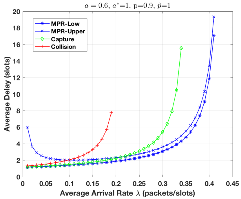

In Fig. 4(b) we present the effect of on the average delay as varies. The cases of the collision, capture and the MPR channel models are presented. As increases then average delay decreases and also the maximum arrival rate that can still maintain a finite delay is getting larger. Clearly, adapting the transmission probabilities depending on the queue state can increase the performance of the system.
IX Conclusions
In this work we considered the case of the two and three-user with bursty traffic in a random access wireless network with a common destination that employs MPR capabilities. We assumed that the users adapt their transmission probabilities based on the status of the queue of the other nodes. For this network we provided the stability region for the two and the three-user case. For the two-user case we provided the convexity conditions of the stability region. Furthermore, we provided a detailed mathematical analysis and derived the generating function of the stationary joint queue length distribution of user nodes in terms of the solution of a two boundary value problems. Based on that result we obtained expressions for the average queueing delay at each user node. For the two-user symmetric case with MPR we obtained a lower and an upper bound for the average delay without explicitly computing the generating function for the stationary joint queue length distribution. The bounds as shown in the numerical results appear to be tight. Explicit expressions for the average delay are obtained for the model with capture effect. Finally, we provided the optimal transmission probability in closed form expression that minimizes the average delay in the symmetric capture case.
Appendix
Intersection points of the curves: In the following we focus on the location of the intersection points of , (resp. ). These points (if exist) are potential singularities for the functions , , and thus, their investigation is crucial regarding the analytic continuation of , outside the unit disk. Note that the analytic continuation of (resp. ) outside the unit disc can be achieved by various methods (e.g., Lemma 2.2.1 and Theorem 3.2.3 in [38]).
Intersection points between , .
Let and , . We can easily show that the resultant in of the two polynomials and is
Note that and due to the fact that and the stability condition (see Lemma III.1).
Similarly, for and , . We can easily show that the resultant in of the two polynomials and is
Note also that since and due to the stability conditions (see Lemma III.1). If , then , and has two roots of opposite sign, say . If , then , and has two positive roots , say (due to the stability conditions). In the former case we have to check if is in , while in the latter case if is in . These zeros, if they lie in such that , are poles of . Denote from hereon
Intersection points between , .
Let and , . It is easily shown that
Thus, , implies that,
The second equation gives . Substituting back in the first one yields, , where Note that , , due to the stability conditions. If , then , and has two roots of opposite sign, say , such that , and for , which in turn implies that , , or equivalently , . In case , , and has two positive roots, say , such that , and for , which in turn implies that , , or equivalently , .
References
- [1] N. Abramson, “THE ALOHA SYSTEM: Another alternative for computer communications,” in Proceedings of the November 17-19, 1970, Fall Joint Computer Conference, AFIPS ’70 (Fall), (New York, NY, USA), pp. 281–285, ACM, 1970.
- [2] A. Laya, L. Alonso, and J. Alonso-Zarate, “Is the random access channel of LTE and LTE-A suitable for M2M communications? a survey of alternatives,” IEEE Communications Surveys Tutorials, vol. 16, pp. 4–16, First 2014.
- [3] A. Osseiran, F. Boccardi, V. Braun, K. Kusume, P. Marsch, M. Maternia, O. Queseth, M. Schellmann, H. Schotten, H. Taoka, H. Tullberg, M. A. Uusitalo, B. Timus, and M. Fallgren, “Scenarios for 5G mobile and wireless communications: the vision of the METIS project,” IEEE Communications Magazine, vol. 52, pp. 26–35, May 2014.
- [4] M. Koseoglu, “Lower bounds on the LTE-A average random access delay under massive M2M arrivals,” IEEE Transactions on Communications, vol. 64, pp. 2104–2115, May 2016.
- [5] J. B. Seo and V. C. M. Leung, “Performance modeling and stability of semi-persistent scheduling with initial random access in lte,” IEEE Transactions on Wireless Communications, vol. 11, pp. 4446–4456, December 2012.
- [6] Z. Utkovski, O. Simeone, T. Dimitrova, and P. Popovski, “Random access in C-RAN for user activity detection with limited-capacity fronthaul,” IEEE Signal Processing Letters, vol. 24, pp. 17–21, Jan 2017.
- [7] H. Wang and T. Li, “Hybrid ALOHA: A novel MAC protocol,” IEEE Transactions on Signal Processing, vol. 55, pp. 5821–5832, Dec 2007.
- [8] Z. Utkovski, T. Eftimov, and P. Popovski, “Random access protocols with collision resolution in a noncoherent setting,” IEEE Wireless Communications Letters, vol. 4, pp. 445–448, Aug 2015.
- [9] C. Stefanovic and P. Popovski, “ALOHA random access that operates as a rateless code,” IEEE Transactions on Communications, vol. 61, pp. 4653–4662, November 2013.
- [10] A. Ephremides and B. Hajek, “Information theory and communication networks: an unconsummated union,” IEEE Transactions on Information Theory, vol. 44, pp. 2416–2434, Oct 1998.
- [11] L. Tong, V. Naware, and P. Venkitasubramaniam, “Signal processing in random access,” IEEE Signal Processing Magazine, vol. 21, pp. 29–39, Sept 2004.
- [12] Y. Gao, C. W. Tan, Y. Huang, Z. Zeng, and P. R. Kumar, “Characterization and optimization of delay guarantees for real-time multimedia traffic flows in IEEE 802.11 WLANs,” IEEE Transactions on Mobile Computing, vol. 15, pp. 1090–1104, May 2016.
- [13] R. Rao and A. Ephremides, “On the stability of interacting queues in a multiple-access system,” IEEE Transactions on Information Theory, vol. 34, pp. 918–930, Sep 1988.
- [14] B. S. Tsybakov and V. A. Mikhailov, “Ergodicity of a slotted ALOHA system,” Problemy Peredachi Informatsii, vol. 15, p. 73–87, 1979.
- [15] W. Szpankowski, “Stability conditions for some distributed systems: buffered random access systems,” Advances in Applied Probability, vol. 26, no. 2, pp. 498–515, 1994.
- [16] W. Luo and A. Ephremides, “Stability of N interacting queues in random-access systems,” IEEE Transactions on Information Theory, vol. 45, pp. 1579–1587, Jul 1999.
- [17] V. Naware, G. Mergen, and L. Tong, “Stability and delay of finite-user slotted ALOHA with multipacket reception,” IEEE Transactions on Information Theory, vol. 51, pp. 2636–2656, July 2005.
- [18] C. Bordenave, D. McDonald, and A. Proutiere, “Asymptotic stability region of slotted ALOHA,” IEEE Transactions on Information Theory, vol. 58, pp. 5841–5855, Sept 2012.
- [19] Y. Zhong, M. Haenggi, T. Q. S. Quek, and W. Zhang, “On the stability of static poisson networks under random access,” IEEE Transactions on Communications, vol. 64, pp. 2985–2998, July 2016.
- [20] A. B. Behroozi-Toosi and R. R. Rao, “Delay upper bounds for a finite user random-access system with bursty arrivals,” IEEE Transactions on Communications, vol. 40, pp. 591–596, Mar 1992.
- [21] L. Georgiadis, L. Merakos, and P. Papantoni-Kazakos, “A method for the delay analysis of random multiple-access algorithms whose delay process is regenerative,” IEEE Journal on Selected Areas in Communications, vol. 5, pp. 1051–1062, Jul 1987.
- [22] K. Stamatiou and M. Haenggi, “Random-access poisson networks: Stability and delay,” IEEE Communications Letters, vol. 14, pp. 1035–1037, November 2010.
- [23] S. Wang, J. Zhang, and L. Tong, “Delay analysis for cognitive radio networks with random access: A fluid queue view,” in IEEE International Conference on Computer Communications, pp. 1–9, March 2010.
- [24] N. Bouman, S. Borst, J. van Leeuwaarden, and A. Proutiere, “Backlog-based random access in wireless networks: Fluid limits and delay issues,” in 23rd International Teletraffic Congress (ITC), pp. 39–46, Sept 2011.
- [25] S. Srinivasa and M. Haenggi, “Throughput-delay-reliability tradeoffs in multihop networks with random access,” in 48th Annual Allerton Conference on Communication, Control, and Computing (Allerton), pp. 1117–1124, Sept 2010.
- [26] S. Srinivasa and M. Haenggi, “A statistical mechanics-based framework to analyze ad hoc networks with random access,” IEEE Transactions on Mobile Computing, vol. 11, pp. 618–630, April 2012.
- [27] F. Poloczek and F. Ciucu, “Service-martingales: Theory and applications to the delay analysis of random access protocols,” in IEEE Conference on Computer Communications (INFOCOM), pp. 945–953, April 2015.
- [28] N. Pappas, M. Kountouris, A. Ephremides, and A. Traganitis, “Relay-assisted multiple access with full-duplex multi-packet reception,” IEEE Transactions on Wireless Communications, vol. 14, pp. 3544–3558, July 2015.
- [29] X. Jian, Y. Liu, Y. Wei, X. Zeng, and X. Tan, “Random access delay distribution of multichannel slotted ALOHA with its applications for machine type communications,” IEEE Internet of Things Journal, vol. 4, pp. 21–28, Feb 2017.
- [30] Z. Chen, N. Pappas, M. Kountouris, and V. Angelakis, “Throughput analysis of smart objects with delay constraints,” in IEEE 17th International Symposium on A World of Wireless, Mobile and Multimedia Networks (WoWMoM), pp. 1–6, June 2016.
- [31] K. Stamatiou and M. Haenggi, “Delay characterization of multihop transmission in a poisson field of interference,” IEEE/ACM Transactions on Networking, vol. 22, pp. 1794–1807, Dec 2014.
- [32] Q. Yao, A. Huang, H. Shan, T. Q. S. Quek, and W. Wang, “Delay-aware wireless powered communication networks energy balancing and optimization,” IEEE Transactions on Wireless Communications, vol. 15, pp. 5272–5286, Aug 2016.
- [33] E. Sandgren, A. G. i Amat, and F. Brännström, “On frame asynchronous coded slotted ALOHA: Asymptotic, finite length, and delay analysis,” IEEE Transactions on Communications, vol. 65, pp. 691–704, Feb 2017.
- [34] W. Szpankowski, “Stability conditions for multidimensional queueing systems with computer applications,” Operations Research, vol. 36, no. 6, pp. 944–957, 1988.
- [35] J. Cohen and O. Boxma, Boundary value problems in queueing systems analysis. Amsterdam, Netherlands: North Holland Publishing Company, 1983.
- [36] G. Fayolle, R. Iasnogorodski, and V. Malyshev, Random walks in the quarter-plane: Algebraic methods, boundary value problems and applications, volume 40 of Applications of Mathematics. Springer-Verlag, Berlin, 1999.
- [37] P. Nain, “Analysis of a two-node aloha-network with infinite capacity buffers,” in Int. Seminar on Computer Networking and Performance Evaluation, pp. 49–63, September 1985.
- [38] G. Fayolle and R. Iasnogorodski, “Two coupled processors: The reduction to a riemann-hilbert problem,” Zeitschrift für Wahrscheinlichkeitstheorie und Verwandte Gebiete, vol. 47, no. 3, pp. 325–351, 1979.
- [39] K. Avrachenkov, P. Nain, and U. Yechiali, “A retrial system with two input streams and two orbit queues,” Queueing Systems, vol. 77, no. 1, pp. 1–31, 2014.
- [40] D. Tse and P. Viswanath, Fundamentals of wireless communication. New York, NY, USA: Cambridge University Press, 2005.
- [41] C. T. Lau and C. Leung, “Capture models for mobile packet radio networks,” IEEE Transactions on Communications, vol. 40, pp. 917–925, May 1992.
- [42] R. Loynes, “The stability of a queue with non-independent inter-arrival and service times,” Proc. Camb. Philos. Soc, vol. 58, no. 3, pp. 497–520, 1962.
- [43] C. T. Lau and C. Leung, “Capture models for mobile packet radio networks,” IEEE Transactions on Communications, vol. 40, pp. 917–925, May 1992.
- [44] M. Zorzi and R. R. Rao, “Capture and retransmission control in mobile radio,” IEEE Journal on Selected Areas in Communications, vol. 12, pp. 1289–1298, Oct 1994.