Performance Analysis of Reliable Video Streaming with Strict Playout Deadline in Multi-Hop Wireless Networks
Abstract
Motivated by emerging vision-based intelligent services, we consider the problem of rate adaptation for high quality and low delay visual information delivery over wireless networks using scalable video coding. Rate adaptation in this setting is inherently challenging due to the interplay between the variability of the wireless channels, the queuing at the network nodes and the frame-based decoding and playback of the video content at the receiver at very short time scales. To address the problem, we propose a low-complexity, model-based rate adaptation algorithm for scalable video streaming systems, building on a novel performance model based on stochastic network calculus. We validate the model using extensive simulations. We show that it allows fast, near optimal rate adaptation for fixed transmission paths, as well as cross-layer optimized routing and video rate adaptation in mesh networks, with less than % quality degradation compared to the best achievable performance.
1 Introduction
Low cost cameras that are able to capture high quality images, combined with increasing wireless transmission rates, and advances in video coding and visual processing are enabling a variety of novel, visual information based intelligent services. The services include vision-controlled robotics [1], automated driving applications [2, 1], and telematic surgery [3], and are often safety critical. Their requirements differ significantly from the ones of traditional video content distribution: they require very low latency, high reliability and good video quality for human inspection or for automated visual processing. As an example, use case specifications for eHealth, future factories and automotive [1, 4] require tens of milliseconds of network, and hundreds of milliseconds of application level delay limits, with a 99.99% reliability. Since the cameras are often hard to access or are mobile, the use of wireless data transmission is inevitable, likely over multiple wireless hops. Multiple wireless hops facilitate the support for multicast or convergecast of the captured streams of images, facilitate handling node mobility, may help to cope with the hostile wireless environment, and could allow low power transmission for battery driven nodes [5, 6, 7].
Scalable video coding (SVC) is an important enabling technology to achieve reliable video streaming in dynamic networking environments [8, 9, 10]. For scalable video coding, each video frame, or group of pictures (GOP), is encoded into multiple layers, and rate adaptation, that is, the selection of an appropriate number of layers to be transmitted, makes it possible to adjust the transmission rate, and thus the video quality to the bandwidth available for the transmission. When the bandwidth of the network path deteriorates, less layers should be transmitted so as to reduce the queuing delays at the intermediate nodes, and to safeguard timely delivery of the layers that are transmitted. At the same time, the transmission of too few layers is detrimental as well, as it leads to high distortion at the receiver.
The traditional approach to rate adaptation with SVC is to follow the long term changes of the transmission rate, either based on the buffer occupancy at the receiver or by estimating the transmission rate [11, 12, 13, 14]. Long term rate adaptation is then combined with buffering at the receiver, so as to even out the short term bandwidth variations. Nonetheless, these rate adaptation solutions cannot be applied for wireless network applications with strict delay limits, as the short term variability of the wireless channels can not be compensated with in-network and receiver buffering. The rate adaptation problem under strict delay constraints is thus particularly challenging and calls for a novel solution approach.
In this paper we attack the problem by proposing model-based rate adaptation for low-latency video streaming in wireless networks, by utilizing a stochastic network calculus approach. A significant advantage of this approach is that it provides quantifiable measures of end-to-end quality of service (QoS) as a function of link quality. These measures can then be translated into useful quality of experience measures (QoE) for the video playout. The QoE measures can then be used for rate adaptation and performance optimization, as well as for the evaluation of new coding schemes.
We utilize the wireless extensions of stochastic network calculus to be able to capture the transmission of the bit stream over the time varying wireless links and the queuing delays at the intermediate nodes [15, 16]. We extend previous results to take the playout process into account, combining two different time scales, the bit-stream-based transmission and queuing and the video-frame-based decoding and playout. We validate the model through extensive simulations, and demonstrate the efficiency of the model-based source rate adaptation and its extension to cross-layer optimized delay sensitive routing.
The rest of the paper is organized as follows. Section 2 discusses recent results on video playout optimization and stochastic network calculus. Section 3 presents background regarding the methodology used. Section 4 describes the considered system. Section 5 presents the model and provides a lower bound on the playout rate under reliability constraint. The model is validated in Section 6, and in Section 7 we evaluate the efficiency of the model-based rate adaptation, including also transmission path optimization. Section 8 concludes the paper.
2 Related Work
As the importance of SVC is widely recognized, scalable extensions of video coding standards are available for H.264/AVC [8], as well as SHVC for H.265/HEVC [9], and new, highly scalable solutions are subject to current research [10]. The objective of SVC is to provide temporal, spatial, and quality scalability by encoding the video stream into multiple layers, a base layer and several enhancement layers, using interlayer processing. As a result, an enhancement layer can be decoded if all previous layers are fully received. The layered structure facilitates a trade-off between video quality (i.e., distortion) and required bandwidth (i.e., rate). This property becomes handy for transmission over wireless and mobile networks [17], where the underlying link quality is subject to the channel variability [18, 20, 19, 21]. The same property makes SVC attractive for delay-limited applications, since all layers received completely before the playout deadline can be utilized for the decoding. Encoding with a larger number of layers increases the potential of more efficient rate adaptation. However, the actual SVC implementation used may limit this potential due to complexity and/or efficiency constraints. Nevertheless, the rapid technological advances may soon render such limitations obsolete. It is therefore important to quantify the performance gains when using a high number of layers in various application domains.
Proposed rate adaptation methods for SVC are based on buffer content [11], transmission rate estimation [12, 13], or both [14], with the advantage that detailed modeling of the network performance is not required. Low delay applications however can not build on buffer-content-based models. Results presented in the literature consider tens of seconds of playout delays. Similarly for low latency requirements, rate adaptation based on average transmission rate would be overly optimistic; it would result in queuing delays at the network nodes and late arrivals at the playout buffer. Therefore, in this paper we propose rate adaptation based on network performance modeling for low latency wireless applications.
Performance modeling of adaptive video streaming in wireless networks has mostly been considered for a single wireless link. In [20] the effect of an unreliable wireless channel is modelled by an i.i.d packet loss process, and the video coding rate and the packet size are optimized under retransmission-based error correction. In [21] and [22] adaptive media playout and adaptive layered coding is addressed respectively. Both papers define a queuing model on a video frame level, assuming that the wireless channel results in a Poisson frame arrival process at the receiving terminal, a simplification that may be reasonable if the buffering at the receiver side is significant, and therefore packet level delays do not need to be taken into account.
Modeling of video streaming based on network calculus is presented in [23] for the purpose of resource allocation in cellular networks, again, considering a frame level model. Modeling of video transmission over two wireless links is presented in [24]. This work considers the video transmission as a bitstream, but even with this simplifying assumption the results reflect that modeling based on traditional queuing theory quickly becomes intractable as the number of links increases. In [25] a tractable model is derived for the delay violation probability for fluid transmission over multihop wireless links, following the effective capacity concept. This approach however does not lend itself to frame level modeling.
In this paper we propose model-based rate adaptation utilizing network calculus. Network calculus characterizes the departure process and the network backlog over multihop paths. Together with recent advances on modeling wireless links, this motivates our approach.
Stochastic network calculus has been extended to capture the randomly varying channel capacity of wireless links, following different methods [26, 27, 28, 29, 15, 30]. Most of the existing work builds on an abstracted finite-state Markov channel (FSMC) model of the underlying fading channel, e.g., [27, 28] or uses moment generating function based network calculus [30]. However, the complexity of the resulting models limits the applicability of these approaches in multi–hop wireless network analysis with more than a few state FSMC model and more than two hops. In this work, we follow the approach proposed by Al-Zubaidy et al [15], where a wireless network calculus based on the dioid algebra was developed. The main premise for this approach is that the channel capacity, and hence the offered service of fading channels is related to the instantaneous received SNR through the logarithmic function as expressed by the Shannon capacity, . Hence, an equivalent representation of the channel capacity in an isomorphic transform domain, obtained using the exponential function, would be . This simplifies the otherwise cumbersome computations of the end-to-end performance metrics.
3 Network Calculus for Wireless Networks
Network calculus has been developed to provide an efficient analytic tool for evaluating the quality of service provided by networks with multi-hop transmission path, including the effect of correlated buffering at the network nodes. In network calculus, the generated network traffic at node in time interval is characterized by the cumulative arrivals, that is, the real–valued non–negative bivariate process , while the transmission capabilities of node are described by the process of cumulative services . The resulting departure process, , characterizes the cumulative traffic leaving node . These processes are non-decreasing in with and for all . The objective of stochastic network calculus is to derive the departure processes for complex network topologies, and based on that express the network performance, typically in terms of probabilistic bounds on the end-to-end delay , and the backlog , characterizing the amount of traffic delayed in the transmission queues of the network. Network calculus can be used to analyze networks with either packetized or fluid flow traffic and for discrete or continuous time scale. In this work, we consider fluid flow traffic and discrete (slotted) time.
Introduced in [15], the network calculus transforms the problem into an alternative domain, called SNR domain, where the SNR service process () is obtained by taking the exponent of the original service process11 1 We use the calligraphic upper–case letters to represent traffic and service processes in the SNR domain and to distinguish them from their bit domain (where traffic and service are measured in bits) counterparts., i.e., . Therefore, we refer to a network element as dynamic SNR server, if it offers a service that satisfies the input–output inequality [31], , where the convolution and deconvolution are respectively defined for any two SNR processes and as
The key result of network calculus is the possibility to substitute the sequence of service processes on a multi-hop transmission path with a single network service process, , by concatenating the service processes for all nodes along a path [32]. In the SNR domain
| (1) |
In addition, network performance bounds, e.g., end-to-end delay and backlog, can be obtained in terms of the deconvolution of the SNR arrival and service processes [15].
The computation of the convolution and deconvolution operations are not straight forward as it involves the evaluation of products and quotients of random processes. Thus, an exact solution for (1) may not be feasible. Instead, we may use yet another transform, the Mellin transform, to find bounds on these two operations. The Mellin transform, see [33], is defined for a nonnegative random variable as , for any complex valued given that the expectation exists. Then, the following holds [15]:
Lemma 1.
Let and be two independent SNR service processes. The Mellin transform of , for all , is bounded by
| (2) |
The Mellin transform of , for , is given by
| (3) |
Lemma 1 above suggests that the Mellin transform of the convolution/deconvolution of two independent processes is bounded by a function of their Mellin transforms. In the case of wireless networks, the independence follows from the assumption on independent fading on the consecutive wireless links. Consequently, network performance bounds can be obtained in terms of the Mellin transforms of the SNR arrival and service processes of that network.
4 System Model and Problem Formulation
In this section we describe our model of the wireless network and of video streaming, formulate the rate adaptation and routing problem, and provide the corresponding arrival and service models.
4.1 Wireless network model
We consider a time slotted multi-hop wireless network with a time slot duration of . We use to refer to a time slot. For each wireless link we consider a block fading channel [34] with Rayleigh fading distribution, with coherence time larger than . As our focus is not on channel coding, we assume that a channel coding scheme is available at each node, such that each channel provides a service that is equivalent to its instantaneous Shannon channel capacity, bits/s, where is the channel bandwidth, is the instantaneous SNR at the receiver of channel at time slot , and we consider that , where denotes equal in distribution, with average . We allow the average SNR to change over time, but we make the reasonable assumption that it is known. Feedback of the channel state information (CSI) over a single link is implemented or can be implemented in modern networks [37, 38], while the CSI or estimated SNR values can be collected in a mesh network with the help of the routing protocol [39].
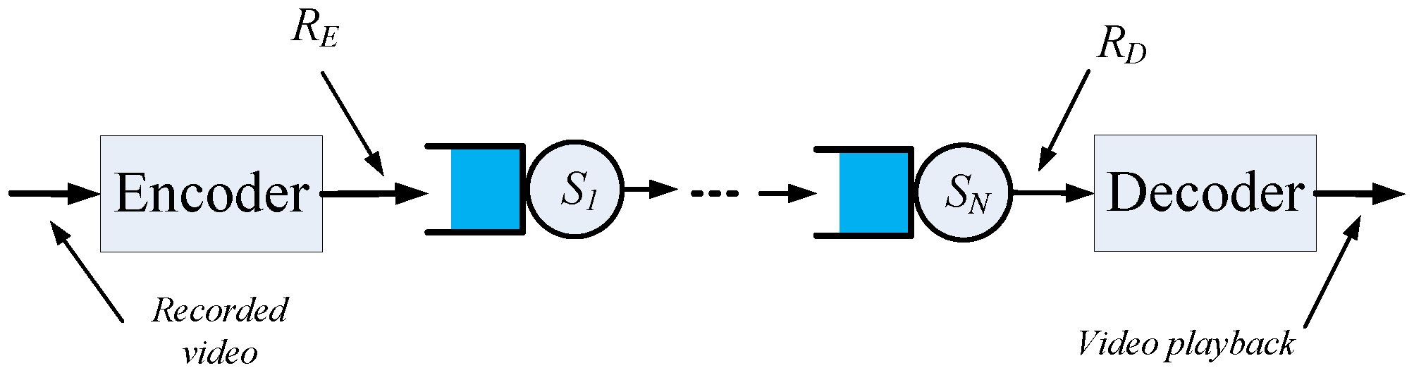
We consider that video has to be streamed between two nodes in the wireless network, as shown in Fig. 1. We refer to a sequence of links from the sender to the receiver node as a transmission path, and denote it by . Furthermore, we denote by the length of the path. There may be multiple paths between the sender and the receiver. We assume that buffers at intermediate nodes are locally FIFO, i.e., frames and their contents are served according to the order of their arrival. Furthermore, no dropping or duplication of contents is allowed at these nodes.
4.2 Scalable video streaming
The video is captured at a rate of frames per second. Depending on the considered coding scheme, a frame can represent a single image, or a group of pictures (GOP). The captured frames are fed directly to the SVC encoder that generates layers. We consider that each layer has a size of bits and a header of bits, resulting in a constant rate traffic of bits per second, where is the frame size in bits, and is determined by the number of transmitted layers . The assumption of equal size layers and constant rate traffic is desirable for ease of presentation, but the proposed methodology can handle any type of traffic, including variable rate video, as long as its Mellin transform exists and is attainable.
The coded video frames are transmitted over a wireless network of transmission links. Once transmitted over the wireless network, received bits are stored in a playout buffer. Frames are decoded and played out regularly with time intervals and a fixed playout delay , that is, a frame that is generated at time is played out after a fixed delay at time . According to the layered coding only the completely received layers are used for decoding. Due to the variability of the wireless channels, the number of layers of a frame that are received within a deadline is random, leading to a varying per frame playout bitrate at the decoder, and consequently varying distortion.
4.3 Model-based rate adaptation and routing problem
Given the system model presented above, the objective of the model-based rate adaptation and routing problem is to select the optimal number of transmitted layers and the optimal transmission path that together maximize the lower bound of the playout rate under a reliability constraint :
| (4) | |||||
| s.t. | |||||
| (5) |
Due to the variability of the wireless channels and the queuing at the intermediate nodes, there is no tractable analytic expression for the distribution of . Therefore, in the following we provide a bound on the tail distribution of , as a function of the frame size, the average SNR values and the path length . We then show how to use it for solving the model-based rate adaptation and routing problem.
4.4 Arrival and Service Models
Recall that is the bitrate of the coded video, and is thus the arrival rate to the wireless network. We can then express the cumulative arrival process as
| (6) |
and the SNR arrival process is given by
| (7) |
Hence, the Mellin transform of the arrival process can be expressed as
| (8) |
Similarily, we can define the cumulative service process of a fading channel with SNR is
| (9) |
Its SNR domain counterpart is given by the log-free form
| (10) |
The Mellin transform of depends on the distribution of , i.e., the fading distribution. In Section 5.3, we will derive the Mellin transform of the service process for Rayleigh channels.
4.5 Service Model with Interfering Flows
The service model presented above for a single flow can be extended to capacity sharing between flows. Let us denote by the SNR arrival process of the tagged (through) flow, and by that of the other (cross) flows. We can then describe the service offered to the through flow by the leftover service process, which can be characterized as shown in Lemma 2 taken from [16].
Lemma 2.
Consider a network with a through flow and cross traffic flow . Assume that the network provides a dynamic SNR server to the aggregate of the two flows, with service process then
is a dynamic SNR server satisfying for all that
The proof of Lemma 2 can be found in [16]. In the rest of the paper, for notational simplicity, we consider that there is no cross traffic.
5 Performance of Video Communication
In this section we present our main contribution: A system model for adaptive video transmission over a multi-hop wireless network and a bound on the received video quality in terms of the parameters of the transmitted video, as well as the underlying fading channels’ parameters. We first derive a general expression on the lower bound of the received rate under playout delay constraint and frame based transmission. Then we give the bound for transmissions over multihop wireless channels, specifically considering Rayleigh fading. Finally we derive the bound on the playout bitrate, considering the layered structure, and address the feasibility of solving the optimal rate adaptation problem.
5.1 Lower Bound for the Received Rate
We investigate a video decoder which operates as follows: At time it considers the content of the playout buffer. It then drops all content that belongs to frames (i.e., late arrivals from previous frames), then removes and decodes all frame content that belongs to frame ; arrivals from subsequent frames remain in the playout buffer. The modelling challenge is twofold. First, the received rate should include only data that belongs to a given frame. Second, we would like to derive a lower bound of the received rate , while network calculus usually considers its upper bound to characterize backlog and delay.
A statistical description of the rate at the decoder, , can be obtained by observing the departure process of the wireless network, . Specifically, can be obtained by considering all departures during the time period from frame generation until playout, that is, , and then counting only , the part of the traffic that belongs to frame . Since the instantaneous received rate at the decoder, , includes only traffic that belongs to fully received layers by the frame’s playout deadline, we can write
| (11) |
A probabilistic lower bound on the departures belonging to frame during the period , , is given by the following lemma.
Lemma 3.
Given a frame generated at time and destined to a decoder with playout deadline , the departure process , is characterized as follows
| (12) |
for all and all .
It is worth noting that this probability is equal to 1 for all , i.e., departures belonging to a frame can never exceed the frame size.

Proof.
Fig. 2 shows the encoding, transmission, and decoding of the consecutive frames and can be used to derive . We express by first considering all departures and then removing traffic that does not belong to frame . As shown in Fig. 2, the departures belonging to previous frames within the interval are equal to the backlog at time , i.e., the traffic from all previous frames that is still in the network when the frame arrives. Once we remove the remaining departures belong to frame , up to a size of , followed by traffic from subsequent frames. Using this argument we arrive at the following equivalence statement
| (13) |
for all .
Lemma 3 states that a probabilistic lower bound for can be obtained in terms of the probabilistic lower bound on the departure process given by (14), for the specific arrival process described in (6). When the arrival and service processes have stationary increments, which is the case here, then is identically distributed for all . The next step is to derive this bound, which we can accomplish using network calculus.
Lemma 4.
For any work-conserving server with dynamic bivariate service process and an arrival process , the departure process is bounded as
| (15) |
where denotes the convolution.
Proof.
Using Reich’s recursive backlog formula we have
where are the instantaneous arrival, service and backlog at time slot respectively. Hence,
where in the second step we used the fact that .
But due to causality we also have
Then for work-conserving server and for we get
Since , and since
Then, and the lemma follows. ∎
5.2 Departure Process Lower Bound for Wireless Channels
To use Lemma 4, we must evaluate the right hand side of (15) which is not an easy task for a wireless channel where is a randomly varying process due to random fading. Therefore, with the following theorem we provide a probabilistic bound on in terms of the Mellin transform of the arrival and service process by using the network calculus approach [15].
Theorem 1.
Let be the SNR arrival process to a work-conserving queuing system with SNR service process , then for any and any , a lower bound () for the departure process must satisfy the following inequality
| (16) |
Proof.
We start by formulating a probabilistic lower bound on the departures in terms of the SNR departure process , , as follows
| (17) |
where we used the assumption to obtain the second line and then we applied Markov’s inequality and used the definition of the Mellin transform to arrive at the last step.
Using Lemma 4, the SNR departure process can be bounded as follows
| (18) |
where we used the definition of the convolution in the last step.
Note that when , the Mellin transform is order-preserving. On the other hand, when , the order is reversed [15]. Hence, the Mellin transform for the SNR departure process for any is computed using (18) as follows
| (19) |
where we used the non-negativity of and and their independence and then we applied the union bound in the last step.
5.3 Lower Bound for Multihop Rayleigh Channels
We will now use Theorem 1 to obtain a probabilistic lower bound on the departure process for an -hop wireless network subject to Rayleigh fading. For simplicity, we present results for the case when for for the hops, but the methodology works for non-identically distributed channel fading using a more complex representation of the network service process as shown in [35].
The instantaneous SNR of a Rayleigh fading channel is exponentially distributed with average . Then the Mellin transform for the cumulative service process of a Rayleigh fading channel defined in (10) is given by [15]
| (20) |
where is the incomplete Gamma function.
Theorem 2.
A probabilistic lower bound on the departure of -hop i.i.d. Rayleigh channels with average SNR , when the arrival process is given by (6), and for is
| (21) |
whenever the stability condition
| (22) |
is satisfied.
Proof.
Let the service offered by a network of store and forward nodes be characterized by the SNR service process . Then using Theorem 1 we obtain for all
| (23) |
A bound on for i.i.d. Rayleigh fading channels is obtained by using the server concatenation property (1) and then applying the convolution bound in Lemma 1 repeatedly times. Then substituting (20) we have for all
| (24) |
The binomial coefficient is the result of expanding the sums and then collecting all terms for the i.i.d channels case [16].
Substituting (6) and (24) in (23) we obtain the following probabilistic lower bound
| (25) |
where, we use the change of variables , let and define .
Using the binomial identity
for all and , the sum in (25) converges to the following
for all , whenever the condition is satisfied. Optimizing over results in the best possible bound and concludes the proof. ∎
5.4 A Bound on Playout Bitrate
Combining the results obtained in Lemma 3 and Theorem 2 for stable system operation we can compute a lower bound on the departures for all as follows
| (26) |
if , otherwise, i.e., if , .
To obtain the lower bound on the departures such that , we equate the right hand side of (26) to and solve for to get
| (27) |
Using (27), the distribution of the number of usable bits (i.e., bits received within the frame’s playback deadline, ) per second is bounded by
where
| (28) |
For steady state operation this corresponds to the decodable rate per frame.
Note that the right hand side of (28) reduces to when , i.e., all layers of the frame are received within the playout deadline . This can happen when the underlying wireless links have high channel quality during the frame transmission, and it represents the best distortion performance that can be achieved for the given coding scheme.
5.5 Effect of on Received Video Quality
The allowable playout delay has a noticeable effect on the received video quality, as stated in the following corollary.
Corollary 1.
The lower bound on the per frame departures increases linearly in the playout deadline , independently from the network and channel conditions, and of the violation probability requirement.
5.6 Optimal rate adaptation and routing
The bounds (26) – (28) characterize the effects of the system parameters on the overall system performance, under the considered Rayleigh fading process with given . Based on these results, we now show how to solve the optimal rate adaptation and routing problem (4)-(5).
The selection of the optimal number of layers per frame and transmission path requires the evaluation of the right hand side (RHS) of (27) for all possible paths . As is convex in , the number of layers per frame, the RHS of (27) can be shown to be concave in . It can also be easily shown that is convex in whenever (see [36]) and hence, in the RHS of (27) is concave in . Therefore, for each path the optimal and the corresponding bound can be obtained via a binary search.
6 Model validation and performance evaluation
The analytic model described in Section 5 provides a lower bound on the per frame departures within the playout deadline . Therefore, we first validate the bounds via simulation. Then, we evaluate the effect of the network and video streaming parameters on the received quality, based on the results in (26) and (27). The effect of have been addressed by Corollary 1.
We consider an SVC scheme that encodes group of pictures (GOP), that is, a frame in the analytic model represents a GOP. One GOP consists of 10 video images. 25 images are generated per second, which results in frames per second. The video is coded with to layers of size kbits of video payload each, resulting in a per frame payload of Mbits, and a video transmission rate of Mbps. For simplicity, we consider , since the typical header size is much smaller than the size of a layer. The playout deadline is msec, which corresponds to a strict delay constraint for real-time machine-to-machine video delivery. We consider transmission paths of links, a channel of bandwidth MHz and average SNR of the fading channels in the range of . This corresponds to average channel capacities of Mbps. We choose a slot duration of msec.
We ran the simulations for a period of time slots, which allows empirical evaluation of the system performance up to a violation probability of .

Fig. 3 shows the CDF of the per frame departures , not yet considering the effect of the layering at the decoding, for and for various transmitted frame size and average channel SNR values. For reference, the channel utilization for the case Mb is under dB, and is for dB.
The figure confirms that the model provides a lower bound on the number of bits received per frame, and shows that the empirical CDF shows the same exponential increase as the model-based lower bound. This exponential growth in can clearly be observed from (26). The bound is tight for low and moderate load, but acceptable even for high utilization of , specifically, the gradient for the model and simulation based results are equal which means that the error diminishes as grows smaller.
We notice that reducing utilization, e.g., by reducing frame size for a given SNR, results in sharper curves, which means that the channel impairments have smaller effect on the video quality. On the other hand, the figure shows that high utilization may lead to overload and low received quality, see for example the utilization case of and , where the probability of receiving even is close to zero. These results reflect well that allowing transmission rates close to the average channel capacity would lead to overload and low quality streaming for latency critical applications.


Figs 4 and 5 evaluate the effect of the channel quality on the received video performance. Fig. 4 shows for and for various and , that the violation probability for given decreases almost exponentially when increasing the average SNR, as soon as the system becomes stable. Fig. 5 shows how the per hop average SNR affects the per frame departures for a violation probability , for different transmitted frame sizes and number of hops . We can see that the SNR has significant effect on the optimal transmission scheme, for example, at , Mbits provides the best performance among the considered frame sizes, Mbits does not fully utilize the network, while Mbits leads to low quality due to network congestion. We also observe that the effect of number of hops, , is significant at high utilization, but diminishes as , and thus the channel capacity increases.
7 Adaptive video transmission and routing
Our analysis exposes the effect of two extreme network behaviours that influence received video quality, namely, network congestion (at high utilization) due to bad channel quality and/or high frame rate, and network underutilization due to low transmitted frame size. It also shows that the optimal operating point, where the transmitted frame size maximizes the received video quality depends on the channel conditions and on the length of the transmission path. Since the wireless channel quality may vary with time, the optimal performance can be achieved by adapting the transmitted frame size to the SNR of the corresponding channels. It may also be beneficial to adapt the routing to the underlying channel quality. In this section, we examine both scenarios and provide examples to illustrate the benefits of such adaptation.
To evaluate the effect of under utilization as well as system overload, Fig. 6 shows the departures per frame, , that fulfill the violation probability limit , as a function of the transmitted frame size , for different SNR values and number of hops.
The figure shows that the frame size leading to maximum departures per frame depends on both of the network parameters. Increasing the frame size above this maximizing value leads to fast quality degradation as the network becomes more saturated. In this figure we also show the effect of layered transmission compared to its fluid counterpart, considering layer size of kbits. As layering affects both the possible transmitted and received frame sizes, we can see performance degradation of a maximum of one layer size. Moreover, we can see that the same performance can be achieved under a range of transmitted frame sizes, which means that an adaptation algorithm would have to find the smallest value to maximize the performance under the lowest transmission rate and thus lowering the energy consumption.
Fig. 7 compares the achieved violation probabilities as a function of the transmitted frame size , for different per frame departure values and SNR values , showing the analytic upper bounds as well as the simulation results. Again, we see that there is an optimum that minimizes . This optimum depends significantly on , and slightly also on the aimed received quality . The simulation results reflect that even though the model overestimates the violation probability, the model-based optimization suggests values close to the real optimum, found via simulation. Consider for example and . The model predicts that Mbits can be achieved with the required reliability with Mbits, while according to the simulation results, the combination Mbits, Mbits is possible too. That is, the model-based parameter selection leads to % bitrate loss only, despite the slacknesss of the violation probability bound.


Fig. 7 also shows a rapid increase in the violation probability when moving away from the optimum frame size. Therefore, the availability of a large number of enhancement layers is critical for a fine-grained rate adaptation to channel conditions, subject to reliability constraints. This becomes never more critical than in applications that require reliable video streaming under low playout deadline, e.g., remote surgery, control of unmanned vehicles.
Fig. 8 summarizes the achievable performance for different expected received frame size values , SNR and number of hops. We see that the range of transmitted frame sizes that yield acceptable violation probability depends on on one side, and on on the other side. The optimal frame size is determined by these two parameters, while the number of hops, , affects significantly the achievable violation probability, but not the optimal value of the frame size.
In order to examine the efficiency of model-based frame size adaptation, we consider adaptation over a fixed transmission path and cross-layer optimized routing and rate adaptation. We compare the proposed model-based adaptation (MOD) to the optimal adaptation (OPT), where the optimum transmission frame sizes, and the resulting per frame departures are obtained by conducting extensive simulations. On Figures 9 and 10 we show the transmitted and received frame size and for OPT. For MOD we show the transmitted frame size that is suggested by the model, the bound on the received frame size, and the actual received frame size where the reliability constraint holds, derived through simulations.

Fig. 9 considers fixed routing with , and layered coding with 100 kbits layer sizes. We consider a scenario where the SNR changes from 10 dB to 6 dB and back to 10 dB at times seconds and seconds respectively. We use results similar to the ones reported in Fig. 7 to demonstrate the frame size adaptation in time. We assume that both the OPT and the MOD based schemes have stabilized at . OPT transmits with a frame size of Mbits, and receives a frame size of Mbits with violation probability . The model-based scheme slightly underestimates both and , but due to the layering, it reaches the same actual per frame departures as the OPT solution. After the channel quality degradation, the MOD scheme decreases , maintaining the system stability, again operating slightly below the OPT scheme. These results demonstrate that albeit the proposed network calculus based model provides only a lower bound on the per frame departures under some quality constraints, it enables the determination of a near optimal transmission frame size as it was suggested by Fig. 7.
In a real implementation of the model-based scheme, the channel quality change would be followed by a transient phase, where the average SNR value is gradually updated, leading to a period with lower than optimal performance. The characterization of this transient phase is out of the scope of the paper.

Finally, Fig. 10 demonstrates an example of rate adaptation combined with routing. We assume that the source node receives routing information, including the per link SNR values periodically, for example every 30 seconds as suggested for the RPL standard [39]. Between routing updates, the source performs rate adaptation based on the SNR feedback on the actual path. We consider the case when the quality of the single hop path deteriorates from dB to dB at seconds, and new routing information is received at seconds, about an path with 10 dB per link SNR. In this case, the longer path provides better service for the delay constrained transmission, as it has also been shown in Fig. 6. As a result, the MOD scheme first adapts to the poor channel quality on the single hop path, it then selects the three-hop path, and increases the transmitted frame size according to the better channel conditions. As the reporting of per hop SNR values, or the minimum SNR perceived on a path can be easily accommodated in routing protocols like RPL, routing combined with the model-based rate adaptation provides an excellent approach to ensure reliable, high quality, delay sensitive video transmission in wireless networks.
8 Conclusion
In this paper we propose a network-calculus-based rate adaptation for delay-sensitive scalable video transmission over multi-hop wireless transmission paths. We derive new network calculus results that provide a probabilistic lower bound on the received video quality while considering the variability of the wireless channels, the effect of the queuing delays at the network nodes and the frame-based playout at the receiver. Our evaluation shows that the channel quality has a more significant effect on the playout performance than the number of hops in the traversed path under low and moderate loads. Nonetheless, the effect of the hop count becomes significant as the network load increases. We show that even if the lower-bound-based model underestimates the achievable reliability, the transmission rate suggested by the model is close to the real optimum. Our results also show that the performance degradation due to the layering effect, compared to the perfect adaptation using the fluid model, depends significantly on the layer size, and hence, the number of enhancement layers per frame. That is, reliable, low latency video streaming over wireless links benefits greatly from adding more layers in layered coding.
The proposed model provides a tool for low-complexity and fast adaptation of the number of transmitted layers to the underlying channel conditions, the playout delay limit and the desired reliability constraints. Our results show that the streaming performance under the model-based rate adaptation is very close to the achievable optimum for various network parameters (within 10% in the considered numerical examples). This suggests that the proposed network-calculus-based approach is an efficient tool for channel-aware rate control and routing for adaptive layered video transmission under strict playout delay limits.
References
- [1] 5G PPP, “5G and the Factories of the Future,” White paper, Oct. 2015.
- [2] M. Gerla, E.-K. Lee, G. Pau, and U. Lee, “Internet of vehicles: From intelligent grid to autonomous cars and vehicular clouds,” in Proc. IEEE World Forum on Internet of Things (WF-IoT), March 2014.
- [3] M. Ghodoussi, S. Butner, and Y. Wang, “Robotic surgery - the transatlantic case,” in Proc. IEEE International Conference on Robotics and Automation (ICRA), May 2002.
- [4] 5G PPP, “5G Automotive Vision,” White paper, Oct. 2015.
- [5] L. Baroffio, et al., “Enabling visual analysis in wireless sensor networks,” in Proc. IEEE International Conference on Image Processing (ICIP), Oct. 2014.
- [6] S. Movassaghi, et al., “Wireless Body Area Networks: A Survey,” IEEE Communications Surveys & Tutorials, vol.16, no.3, pp.1658-1686, 2014.
- [7] H. Nishiyama, M. Ito, N. Kato, “Relay-by-smartphone: realizing multihop device-to-device communications,” IEEE Communications Magazine, vol.52, no.4, pp.56-65, April 2014.
- [8] H. Schwarz, D. Marpe and T. Wiegand, “Overview of the Scalable Video Coding Extension of the H.264/AVC Standard,” IEEE Transactions on Circuits and Systems for Video Technology, vol. 17, no. 9, pp. 1103-1120, Sept. 2007.
- [9] J. M. Boyce, Y. Ye, J. Chen and A. K. Ramasubramonian, “Overview of SHVC: Scalable Extensions of the High Efficiency Video Coding Standard,” IEEE Transactions on Circuits and Systems for Video Technology, vol. 26, no. 1, pp. 20-34, Jan. 2016.
- [10] D. Rüfenacht, R. Mathew and D. Taubman, “A Novel Motion Field Anchoring Paradigm for Highly Scalable Wavelet-Based Video Coding,” IEEE Transactions on Image Processing, vol. 25, no. 1, pp. 39-52, Jan. 2016.
- [11] K. Spiteri, R. Urgaonkar, R. K. Sitaraman, “BOLA: Near-Optimal Bitrate Adaptation for Online Videos,” in Proc. IEEE Infocom, April, 2016.
- [12] L. De Cicco, V. Caldaralo, V. Palmisano and S. Mascolo, “ELASTIC: A Client-Side Controller for Dynamic Adaptive Streaming over HTTP (DASH),” in Proc. International Packet Video Workshop, December 2013.
- [13] Z. Li, X. Zhu, J. Gahm, R. Pan, H. Hu, A.C. Begen and D. Oran, “Probe and Adapt: Rate Adaptation for HTTP Video Streaming At Scale,” IEEE Journal on Selected Areas in Communications, vol.32, no.4, pp.719-733, April 2014.
- [14] X. Yin, A. Jindal, V. Sekar, and B. Sinopoli, “A Control-Theoretic Approach for Dynamic Adaptive Video Streaming over HTTP,” SIGCOMM Comput. Commun. Rev. vol.45 no.4, pp.325-338, August 2015.
- [15] H. Al-Zubaidy, J. Liebeherr, and A. Burchard. “A (min, x) network calculus for multi-hop fading channels,” in Proc. IEEE Infocom, April 2013.
- [16] H. Al-Zubaidy, J. Liebeherr, and A. Burchard, “Network-layer performance analysis of multihop fading channels,” IEEE/ACM Transactions on Networking, vol. 24, no. 1, pp. 204–217, February 2016.
- [17] J. Nightingale, Qi Wang, C. Grecos, “Scalable HEVC (SHVC)-Based video stream adaptation in wireless networks,” in Proc. IEEE 24th International Symposium on Personal Indoor and Mobile Radio Communications (PIMRC), Sept. 2013.
- [18] T. Schierl, T. Stockhammer, and T. Wiegand, “Mobile video transmission using scalable video coding,” IEEE Transactions on Circuits and Systems for Video Technology, vol. 17, no. 9, pp. 1204–1217, Sept 2007.
- [19] S. Chen, J. Yang, E. Yang, and H. Xi, “Receiver-driven adaptive layer switching algorithm for scalable video streaming over wireless networks,” in Proc. IEEE International Conference on Networking, Sensing and Control (ICNSC), April 2014.
- [20] H.-L. Lin, T.-Y. Wu, and C.-Y. Huang, “Cross layer adaptation with QoS guarantees for wireless scalable video streaming,” IEEE Communications Letters, vol. 16, no. 9, pp. 1349–1352, Sept, 2012.
- [21] S. Chen, J. Yang, Y. Ran, and E. Yang, “Adaptive layer switching algorithm based on buffer underflow probability for scalable video streaming over wireless networks,” IEEE Transactions on Circuits and Systems for Video Technology, vol 26, no. 6, pp.1146–1160, June 2016.
- [22] J. Yang, H. Hu, H. Xi, and L. Hanzo, “Online buffer fullness estimation aided adaptive media playout for video streaming,” IEEE Transactions on Multimedia, vol. 13, no. 5, pp. 1141–1153, Oct. 2011.
- [23] A. Rizk and M. Fidler, “Queue-aware uplink scheduling: Analysis, implementation, and evaluation,” in Proc. IFIP Networking Conference, May 2015.
- [24] W. Song, “Delay analysis for compressed video traffic over two-hop wireless moving networks,” in Proc. IEEE Globecom, Dec 2011.
- [25] D. Wu and R. Negi, “Effective Capacity-Based Quality of Service Measures for Wireless Networks,” Mobile Networks and Applications, vol. 11, no. 1, pp. 91–99, February 2006.
- [26] F. Ciucu, “Non-asymptotic capacity and delay analysis of mobile wireless networks,” in Proc. ACM Sigmetrics, June 2011.
- [27] M. Fidler, “A network calculus approach to probabilistic quality of service analysis of fading channels,” in Proc. IEEE Globecom, Nov. 2006.
- [28] K. Mahmood, A. Rizk, and Y. Jiang, “On the flow-level delay of a spatial multiplexing MIMO wireless channel,” in Proc. IEEE ICC, June 2011.
- [29] G. Verticale and P. Giacomazzi, “An analytical expression for service curves of fading channels,” in Proc. IEEE Globecom, Nov. 2009.
- [30] M. Fidler, “An end-to-end probabilistic network calculus with moment generating functions,” in Proc. IEEE IWQoS, June 2006.
- [31] C.-S. Chang. Performance guarantees in communication networks. Springer Verlag, 2000.
- [32] Y. Jiang and Y. Liu. Stochastic network calculus. Springer, 2008.
- [33] B. Davies, Integral transforms and their applications, Springer-Verlag, NY, 1978.
- [34] R. McEliece and W.E. Stark. “Channels with block interference,” IEEE Transactions on Information Theory, vol. 30, no. 1, pp.44–53, Jan 1984.
- [35] N. Petreska, H. Zubaidy, R. Knorr, and J. Gross, “On the recursive nature of end-to-end delay bound for heterogeneous wireless networks,” in Proc. IEEE ICC, June 2015.
- [36] N. Petreska, H. Zubaidy, R. Knorr, and J. Gross, “Power-minimization under statistical delay constraints for multi-hop wireless industrial networks,” arXiv:1608.02191v2 [cs.PF], Aug. 2016.
- [37] D. Halperin, W. Hu, A. Sheth, and D. Wetherall, “Tool release: gathering 802.11n traces with channel state information,” SIGCOMM Comput. Commun. Rev. vol.41, no.1 Jan. 2011.
- [38] E. Dahlman, S. Parkvall and J. Sköld, “4G LTE/LTE-Advaned for Mobile Broadband.” Academic Press, 2011.
- [39] N. Accettura, L. Grieco, G. Boggia, and P. Camarda, “Performance analysis of the RPL routing protocol,” in Proc. IEEE International Conference on Mechatronics (ICM), April 2011.