DESY 14-096
Low-lying baryon masses using twisted mass clover-improved fermions directly at the physical point
C. Alexandrou(a,b), C. Kallidonis(b)
(a) Department of Physics, University of Cyprus, P.O. Box 20537,
1678 Nicosia, Cyprus
(b) Computation-based Science and Technology Research Center, The Cyprus Institute, 20 Kavafi Str., Nicosia 2121, Cyprus
The masses of the low-lying baryons are evaluated using an ensemble with two degenerate light twisted mass clover-improved quarks with mass tuned to reproduce the physical pion mass. The Iwasaki improved gluonic action is employed. The coupling constant value corresponds to a lattice spacing of fm, determined from the nucleon mass. We find that the clover term supresses isospin symmetry breaking as compared to our previous results using twisted mass fermions. The masses of the hyperons and charmed baryons evaluated using this ensemble are in agreement with the experimental values. We provide predictions for the mass of the doubly charmed , as well as of the doubly and triply charmed s that have not yet been determined experimentally.
August 24, 2026
Keywords:
Hyperon and charmed baryons, Lattice QCDpacs
11.15.Ha, 12.38.Gc, 12.38.Aw, 12.38.-t, 14.70.DjI Introduction
Baryon masses of all low-lying hyperons and singly charmed baryons are well known from experiments [1], and they therefore serve as benchmark quantities for lattice QCD calculations. In contrast, the doubly and triply charmed sector remains mostly unexplored experimentally, though predicted by QCD and the quark model. The only available experimental evidence of doubly charmed baryons is the SELEX report of five resonances, identified as , , , and [2, 3]. The state was later confirmed by SELEX [4, 5], having a mass of GeV and an average lifetime less than 33 s. This discovery has triggered a revival of the interest in charmed baryon spectroscopy. However, the fact that these resonances have not been confirmed by either the BABAR [6], Belle [7, 8], LHCb at CERN [9] and FOCUS [10] experiments is somewhat puzzling. What adds to the puzzle is that theoretical studies, e.g. QCD sum rules [11] as well as relativistic [12, 13] and non-relativistic [14] quark models predict the mass to be 100-200 MeV higher than what SELEX has observed. This deviation is also confirmed by lattice QCD predictions, as discussed in Section III.2. Even more interesting is the isospin splitting of about MeV between the and the states, which is one order of magnitude larger when compared to the mass differences of the other isospin partners. A possible explanation for this is that the Coulomb electro-magnetic effect dominates the strong interaction effect, hence these baryons have a very compact size [15]. Future experimental activity on heavy baryon spectroscopy, such as the Beijing Spectrometer (BES-III) [16], the LHC [17, 18, 19], the Belle-II [20] and PANDA [21] is expected to shed more light into the existence on doubly and triply charmed baryons.
Lattice QCD is in a good position to investigate the masses of doubly and triply charmed baryons using simulations with physical values of the quark masses. In view of the ongoing experimental efforts to study charmed baryons, lattice QCD can provide valuable input. A number of lattice QCD groups have studied the ground states of spin-1/2 and spin-3/2 charmed baryons using a variety of lattice schemes, with the most recent ones using dynamical simulations [22, 23, 24, 25, 26, 27, 28, 29, 30]. Many of these calculations perform chiral and continuum extrapolations. Recently, the study was extended to the higher spins of 5/2 and 7/2 and excited states using an ensemble of clover fermions on an asymmetric lattice at a pion mass of MeV [31]. We make a thorough discussion of the various lattice calculations and how they compare with our results and the experimental values in Sec. III.2.
In this work, we use an ensemble generated by the European Twisted Mass Collaboration (ETMC) with two degenerate twisted mass clover-improved light quarks with mass tuned to reproduce the physical pion mass [32]. This thus eliminates systematic uncertainties arising from chiral extrapolations. The clover-term helps in the stabilization of the simulations, while it still preserves the improvement of the twisted mass action [33, 34] and reduces the lattice artefacts related to the breaking of the isospin symmetry. We refer to this gauge ensemble as “the physical ensemble” from now on. This study extends our previous computations on the low-lying baryon spectrum using [35] and [36] twisted mass fermions using higher than physical pion masses.
We use Osterwalder-Seiler valence strange and charm quarks. Since our interest in this work is the baryon spectrum we choose to use the physical mass of the and baryons to tune the strange and charm quark masses, respectively. We also opt to use the nucleon mass to fix the lattice spacing, , in order to convert our lattice values to physical units. Comparisons of our previous results on the masses using and ensembles show no sensitivity to the dynamical strange and charm quarks, at least within the statistical errors of the results. Therefore, as a first study using physical values of the light quark mass we will assume that strange and charm quark unquenching effects are small. This is also corroborated by results obtained using and twisted mass ensembles on quantities such as the strange and charm quark masses [37, 38] as well as the kaon and D-meson decay constants [39, 40], which showed no detectable unquenching effects.
Isospin breaking in the twisted mass formulation is a lattice artefact of order . It has been shown that adding the clover term reduces isospin splitting in the multiplet [32] as compared to the twisted mass simulations at a similar lattice spacing. Here we study the effects of isospin breaking effects to higher accuracy in the -system and in strange and charm sectors. We compare our final results on the masses of the forty baryons studied in this work with those of other recent lattice calculations, using a variety of discretization schemes as well as with experiment. We find remarkable agreement with experimental results even though no continuum extrapolation is performed and provide predictions for the masses of doubly and triply charmed baryons.
The paper is organized as follows: The lattice action employed in the single ensemble we analyze in this work, as well as the details of the calculations, including the interpolating fields, the determination of the lattice spacing and the tuning of the strange and charm quark masses are given in Section II. In Section III we present our lattice results, where we study the effect of isospin symmetry breaking and discuss the various systematics. In section III.2 we compare our values with those from other lattice calculations and with experiment and in Sec. IV we give our conclusions.
II Lattice techniques
II.1 The lattice action and simulation parameters
In this work we analyze a gauge ensemble produced by ETMC at the physical pion mass [32]. The form of the gauge action used in the generation of this ensemble is
| (1) |
where denotes the real part and the parameters and are chosen such that the “Iwasaki” improved gauge action is reproduced [41, 42]. The gauge coupling parameter was chosen to produce a lattice spacing of roughly fm. In the fermion sector the twisted mass fermion action for a doublet of degenerate quark flavours [33, 34] is employed, with a clover-term [43] added.
| (2) |
where is the third Pauli matrix acting in the flavour space, is the bare untwisted light quark mass, is the bare twisted light quark mass and the last term is the clover-term, with the so-called Sheikoleslami-Wohlert improvement coefficient. The field strength tensor is given by [43]
| (3) |
where is a fundamental Wilson plaquette and . The value of appearing in the clover-term of Eq. (2) was set to from Padé fits to data produced by the CP-PACS/JLQCD collaboration [44]. Since the action is already -improved it is not necessary to use the non-perturbative value and any value that minimizes the mass splitting between the neutral and charged pions can be used. It was shown that using reduces the isospin splitting between the neutral and charged pions to zero [32].
In Eq. (2) denotes the massless Wilson-Dirac operator given by
| (4) |
where
| (5) |
The quark fields denoted by in Eq. (2) are in the so-called “twisted basis”. The fields in the “physical basis”, , are obtained for maximal twist by the transformation
| (6) |
In this paper, unless otherwise stated, the quark fields will be understood as “physical fields”, , in particular when we define the baryonic interpolating fields.
Twisted mass fermions (TMF) provide an attractive formulation of lattice QCD allowing for automatic improvement, infrared regularization of small eigenvalues and fast dynamical simulations [34]. However, the lattice artefacts that the twisted mass action exhibits lead to instabilities in the numerical simulations, particularly at lower values of the quark masses and influence the phase structure of the lattice theory [45, 46, 47]. The clover-term is added in the TMF action for stabilizing the simulations with quark masses low enough to reproduce the physical pion mass, while at the same time retaining automatic improvement that the TMF action features.
Maximally twisted Wilson quarks are obtained by setting the untwisted quark mass to its critical value , while the twisted quark mass parameter is kept non-vanishing to give mass to the light quarks. A crucial advantage of the twisted mass formulation is the fact that, by tuning the bare untwisted quark mass to its critical value , all physical observables are automatically improved [34, 48]. In practice, we implement maximal twist of Wilson quarks by tuning to zero the bare untwisted current quark mass, commonly called PCAC (Partially Conserved Axial Current) mass, [49, 50], which is proportional to up to corrections. A convenient way to evaluate is through
| (7) |
where is the axial vector current and is the pseudoscalar density in the twisted basis. The large limit is required in order to isolate the contribution of the lowest-lying charged pseudoscalar meson state in the correlators of Eq. (7). This way of determining is equivalent to imposing on the lattice the validity of the axial Ward identity , , between the vacuum and the charged zero three-momentum one-pion state. When is taken such that vanishes, this Ward identity expresses isospin conservation, as it becomes clear by rewriting it in the physical quark basis.
In Table 1 we list the input parameters of the calculation, namely , , the bare light quark mass as well as the value of the pion mass. As one can see, the calculated pion mass is marginally below the physical pion mass. The value of the lattice spacing is determined from the nucleon mass, as explained in subsection II.4. We analyze 357 gauge configurations, which provide a reasonable statistical accuracy for the observables in question.
| , fm | ||
|---|---|---|
| , fm | 0.0009 | |
| No. of Confs | 357 | |
| (GeV) | 0.130 | |
| 2.98 | ||
II.2 Two-point correlation functions and effective mass
In this work we consider two-point correlation functions, defined by
| (8) |
where is the interpolating field of the baryon state of interest acting at the source, and the sink, . The effective mass is obtained from the time dependence of the two-point function at . In this case, the symmetries of the action and the anti-periodic boundary conditions in the temporal direction for the quark fields imply that , where is the temporal extent of the lattice. Therefore, in order to decrease errors we average correlators in the forward and backward direction and define . In addition, the source location is chosen randomly on the whole lattice for each configuration, in order to decrease correlation among measurements.
The ground state mass of a given baryon is extracted from the effective mass as
| (9) |
where is the mass difference of the excited state with respect to the ground mass . All results in this work have been extracted from correlators where Gaussian smearing is applied both at the source and sink. In general, the effective mass defined by the correlators of a given interpolating field is expected to have the asymptotic value. However, applying smearing on the interpolating fields suppresses excited states, therefore yielding a plateau region at earlier source-sink time separations and thus better accuracy in the extraction of the mass. Our fitting procedure to extract is as follows: The sum over excited states in the effective mass given in Eq. (9) is truncated, keeping only the first excited state,
| (10) |
The upper fitting time slice boundary is kept fixed, while allowing the lower fitting time to be two or three time slices away from . We then fit the effective mass to the form given in Eq. (10). This exponential fit yields an estimate for and as well as for the ground state mass, which we denote by . Then, we perform a constant fit to the plateau region of the effective mass increasing the initial fitting time . We denote the extracted value from the constant fit by . The final value of the mass is picked as the constant fit at the lowest for which the criterion
| (11) |
is satisfied, where is the statistical error on . This criterion is, in most cases, in agreement with becoming less than unity. We show representative results of the effective masses of a number of spin-1/2 and spin-3/2 baryons in Fig. 1, including the exponential and plateau fits. The error bands are obtained using jackknife analysis. As can be seen the exponential and plateau fits yield consistent results in the large time limit. We note that fitting directly the correlators instead of the effective masses yields compatible results. We choose the values extracted from the constant fits on the effective masses as our final baryon masses, quoted in Table 4.


II.3 Interpolating fields
In order to create baryon states on the lattice, we act on the vacuum with appropriate interpolating field operators, constructed such that they have the quantum number of the baryon of interest and reduce to the quark model wave functions in the non-relativistic limit. The forty baryons we analyze in this work consist of combinations of three out of the four quark flavors, , , and , therefore we use SU(3) subgroups of the SU(4) symmetry to construct their interpolating fields. We use the same interpolating fields employed in our previous studies [51, 36, 52]. For completeness we summarize below the constructions of the interpolating fields.
In general, the interpolating fields of baryons can be written as a sum of terms of the form , apart from overall constants. The structures and are such that they give rise to the quantum numbers of the baryon state of interest. For spin-1/2 baryons, we will use the combination and for spin-3/2 baryons we will use , with . is the charge conjugation matrix.
The multiplet numerology is . All the baryons in a given multiplet have the same spin and parity. Briefly, the -plet consists of the spin-3/2 baryon states and can be further decomposed according to the charm content of the baryons into , where the is the standard decuplet and is the triply charm singlet. The singly charmed baryon states belonging to the multiplet are symmetric under the interchange of , and quarks, following the rule that the diquark is symmetric under interchanging . The doubly charmed -plet consists of the isospin partners and the singlet . The -plet is shown schematically in the left panel of Fig. 2. The corresponding interpolating fields of the spin-3/2 baryons are collected in Table 6 of Appendix A.
Similarly, the -plet consists of the spin-1/2 baryons as shown schematically in the center panel of Fig. 2. It can be decomposed as . The ground level where comprises the well-known baryon octet, whereas the first level splits into two SU(3) multiplets, a and a . The states of the are symmetric under interchanging , and where the states of the are anti-symmetric. We show these states explicitly in the right panel of Fig. 2. We note that the diquark appearing in the interpolating field of spin-1/2 baryons is anti-symmetric under interchanging . The top level consists of the -plet with . The interpolating fields of the spin-1/2 baryons are collected in Table 5 of Appendix A. The fully antisymmetric -plet is not considered in this work.


In order to suppress excited state contamination, we apply Gaussian smearing to the quark fields at the source and sink [53, 54], given by , where is the gauge invariant smearing function and is the hopping term realized as a matrix in coordinate, color and spin space,
| (12) |
The parameters and of the Gaussian smearing used in this work are and .
In addition, we apply APE smearing to the spatial links that enter the hopping term. The parameters of the APE smearing we used are and .
The interpolating fields for the spin-3/2 baryons as defined in Table 6 have an overlap with spin-1/2 states. In order to isolate the desired spin-3/2 ground state, we incorporate a spin-3/2 projector in the definitions of the interpolating fields
| (13) |
For non-zero momentum, is defined by [55]
| (14) |
The corresponding spin-1/2 projector is obtained by . In this work we study the mass spectrum of the baryons in the rest frame taking , thus the last term of Eq. (14) will vanish. When the spin-3/2 and spin-1/2 projectors are applied to the interpolating field operators, the resulting two-point correlators for the spin-3/2 baryons acquire the form
| (15) |
where . It turns out that for some of the baryons we study, such as the , the inclusion of the spin-3/2 projector does not have a significant effect in the correlation function. However, we find that it is necessary for some others, such as the , in order to isolate the spin-3/2 ground state. Therefore, in order to ensure that we always measure the desired spin-3/2 ground state, we apply the spin-3/2 projector to all of the interpolating fields of Table 6. The reader interested in more details on the effects of these projectors on the baryon two-point functions and masses is referred to Ref. [36].
II.4 Determination of the lattice spacing
In order to fix the lattice spacing for our physical ensemble, we used the physical nucleon mass as input. For this purpose we carried out a dedicated high statistics analysis of the nucleon mass with around 800,000 measurements, leading to an accurate determination of the lattice spacing. The pion and nucleon mass in lattice units are
| (16) |
yielding a ratio of , which differs by when compared to the physical value of . If we were to assume that we are exactly at the physical point and use the physical value of the nucleon mass we would obtain GeV fm, yielding GeV i.e. 3% smaller than physical. Allowing to be slightly away from the physical pion mass we can perform an interpolation to the physical point as follows: Observing that our previous results using and ensembles showed no detectable cut-off and volume effects nor we have seen any unquenching effects due to the strange and charm quarks in the sea, we make use of the nucleon masses from 17 ensembles [36] in order to interpolate the nucleon mass of the physical ensemble. Namely, we perform a combined fit to the physical ensemble and the 17 ensembles using the SU(2) chiral perturbation theory (PT) well-established expression [56, 57]
| (17) |
We collect the pion and nucleon masses that we used in the fit in Table 7 of Appendix id1. The three lattice spacings of the ensembles, the lattice spacing of the physical ensemble as well as the nucleon mass at the chiral limit, , are treated as fit parameters. The value of is fixed such that the fit curve passes through the physical value of the nucleon mass at physical pion mass (physical point). In order to estimate the systematic error due to the chiral extrapolation, we also perform the fit using heavy baryon chiral perturbation theory (HBPT) to in the small scale expansion (SSE) scheme [58]. This form includes explicit degrees of freedom by introducing as an additional parameter the -nucleon mass splitting, , taking . For completeness, we give the expression for the nucleon mass in the SSE scheme
| (18) | |||||
where for and for . We take the cut-off scale GeV, [58] and treat the counter-term as an additional fit parameter. The physical values of and are used in both fits, namely GeV and . We take the difference between the results of the and fits as an estimate of the uncertainty due to the chiral extrapolation. The final value of the lattice spacing for the physical ensemble is
| (19) |
where the error in the first parenthesis is the statistical error and the systematic error is given in the second parenthesis. This value is in agreement with the value extracted assuming the simulation is exactly at the physical point, which demonstrates that any deviation form the physical point is within the accuracy of the results. From our lattice values of Eq. (16) and using Eq. (19) we find that the pion mass in physical units is GeV, which is about lower than the average physical pion mass, and the corresponding nucleon mass is GeV, less than lower from the physical nucleon mass, which explains the agreement between the two determinations.
In Fig. 3 we show the fits of the nucleon mass to the and expressions of Eqs.(17) and (18), respectively. The error band and the errors on the fit parameters are obtained from super-jackknife analysis [59]. As mentioned above, cut-off effects were investigated in Ref. [36] and were found to be negligible for the nucleon mass. This is corroborated by fitting the data for each of the ensembles separately to extract the lattice spacings. We find that the values are in agreement with those from the combined fit. We note that our lattice results exhibit a curvature, which supports the presence of the -term. We remark here that by including the nucleon mass from the physical ensemble in the fit, the lattice spacings of the ensembles as well as the rest of the fitting parameters remain completely unchanged. In addition, if we fit using ensembles by ETMC [60, 61] instead of the ensembles we obtain the same result as in Eq. (19) for the physical ensemble, and the lattice spacings for the ensembles have the same values, as if we fitted without the physical ensemble. These are indications that the interpolation carried out is very robust. The fit parameters for the two fits including the /d.o.f. are given in Table 2. For completeness, we give the lattice spacings for the ensembles
| (20) |
where the error in the first parenthesis is statistical and in the second parenthesis the systematic due to the chiral extrapolation, as explained above.
| (GeV-3) | (MeV) | ||||
|---|---|---|---|---|---|
| HBPT | 0.8667(15) | 4.5735 | 64.9(1.5) | 1.5779 | |
| SSE | 0.8813(47) | 3.7282 | -2.5858(2480) | 51.7(4.3) | 1.0880 |
Finally, we note that the value of Eq. (19) is fully consistent with the one determined from gluonic quantities, from , and the ones related to the action density renormalised through the gradient flow. It is, however, larger by about 2% as compared to the one extracted using and [32]. We will use the lattice spacing given in Eq. (19) to convert to physical units all the quantities studied in this work.
Having determined the parameters of the chiral fit we can compute the nucleon -term by evaluating where we have taken the leading order relation . Using Eq. (17) we find MeV. Performing the same calculation using the expression we obtain a lower value of MeV showing the sensitivity of this quantity to the chiral extrapolation. As with the fit parameters, the values of -term are unchanged by including the nucleon mass at the physical ensemble in the fits [36]. We note that these values are larger as compared to direct evaluations of this quantity by a number of lattice QCD groups including one performed using this ensemble [62], where a value of MeV was obtained. Given the large variation when using the two different chiral expansions, the evaluation of from the slope of the fit receives a large systematic error of 13.2 MeV, giving a value of MeV, which brings the disagreement with the direct determination to one standard deviation.
II.5 Tuning of the bare strange and charm quark masses
In order to determine the bare strange and charm quark masses, we perform a tuning using the physical mass of the (1.672) baryon and the (2.286) baryon, respectively, as input. Our strategy is to calculate the and masses at various trial values of and and then match directly with the physical and mass, respectively, assuming small cut-off and finite volume effects. This procedure determines the tuned values of and . In Fig. 4 we show the matching of the strange and charm quark masses with the physical and masses, respectively. The values of and used for the tuning, along with the respective and masses are listed in Table 3. An analysis using the same ensemble as the one we are using here yielded and from interpolation of the meson mass ratios and [32], showing an agreement within 4% and 7%, respectively, when compared to our results. This is very satisfactory given that systematic errors are not included. Since we interested in the baryon sector we use the tuned quark mass values determined from using baryonic observables. The tuned values we find for the bare heavy quark masses are
| (21) |
where the error is the statistical, obtained from the fit band. From these values we find and . Our analysis using the meson mass ratios and for the same ensemble as the one we are using here are and [32]. These ratios are about a standard deviation different from the ones we find in this work, indicating that systematic errors on these ratios from using different quantities to fix the quark masses are small and comparable with the statistical ones.
The renormalization constant is determined for this ensemble non-perturbatively. We find in the at 2 GeV [63], where the first error is statistical, the second is a systematic error stemming from the extrapolation to and the perturbative subtraction of leading lattice artefacts, and the third from the conversion of RI′-MOM to at 2 GeV. Using this value of and the lattice spacing of Eq. (19), the renormalized strange and charm quark masses are
| (22) |
where the first error is statistical, the second the combined systematic error from the determination of and the lattice spacing of Eq. (19) and the third from the conversion of RI′-MOM to at 2 GeV. The corresponding renormalized masses determined from meson mass ratios and for the same ensemble are MeV and GeV in the at 2 GeV [32] with the errors being determined in the same manner as in Eq. (22). These renormalized strange and charm quark masses are in agreement with the values given in Eq. (22). A more complete analysis, including systematic errors due to lattice artefacts will follow in the future.
It is interesting to compare our values of the strange and charm quark masses with the ones given by the FLAG group. The FLAG ratios are and [64]. The FLAG values are continuum extrapolated and corrected for finite volume effects. The fact that our values are within one standard deviation for the and two standard deviations for the is very satisfactory. Furthermore, the and values obtained by the FLAG are [64]
| (23) |
in the , where the value for resulted from an analysis using twisted mass ensembles from the meson sector [37]. The strange renormalized mass quoted by FLAG is consistent with our value determined from the at this fixed lattice spacing. The renormalized charm quark mass is smaller by two standard deviations, which is rather satisfactory given that our value is obtained for one ensemble with no evaluation of cut-off effects.

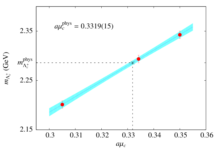
| (GeV) | (GeV) | ||||
|---|---|---|---|---|---|
| 0.0232 | 0.7793(31) | 1.6375(65) | 0.3050 | 1.0475(36) | 2.2012(75) |
| 0.0245 | 0.7872(30) | 1.6541(64) | 0.3342 | 1.0915(36) | 2.2936(76) |
| 0.0280 | 0.8084(29) | 1.6987(61) | 0.3500 | 1.1149(37) | 2.3427(77) |
III Lattice Results
III.1 Isospin symmetry breaking
The breaking of the isospin symmetry is a feature of the lattice twisted mass fermion action due to the presence of acting in flavor space. Isospin breaking effects are of the order and in general they are detectable as mass splittings between hadrons belonging to the same isospin multiplets. Possible isospin splitting effects should vanish in the continuum limit. There is still an exact symmetry of the twisted mass action, namely parity combined with an interchange of u- and d-quarks, according to which the proton and the neutron are degenerate, as are the , and the , baryons. However, there could be a mass difference between, e.g. the and the baryons. Therefore, we average over the masses of the proton and the neutron, as well as the , and , . In the latter case, we take the difference between the two averages to study isospin splitting effects. We extend the isospin breaking study for all isospin multiplets of the forty baryons we analyze in this work. In all figures concerning isospin splitting, we additionally show the corresponding splitting for the ensembles, analyzed in a previous work [36] for comparison.
We start this analysis by showing the mass difference for the octet and decuplet isospin multiplets, shown in Fig. 5. In the octet case there are small mass splittings in the and baryon multiplets, which amount to about of the mass of the baryons at the isospin limit. This splitting is taken as a systematic error in our final results for the and baryons. It is also notable that the breaking is more than twice smaller when compared to the corresponding ones obtained using the ensembles at similar value of the lattice spacing, which confirms that combining Wilson twisted mass fermions at maximal twist and the clover term reduces cut-off effects related to isospin symmetry breaking. Regarding the decuplet, the mass difference in the , and isospin multiplets is consistent with zero within our statistical accuracy, indicating that isospin splitting effects are minimal in this case.
In the charm sector, we show the mass difference of the spin-1/2 , , and multiplets in the left panel of Fig. 6. As can be seen, the mass splitting is consistent with zero for all states except , where a mere splitting is observed. As with the decuplet, the charm spin-3/2 multiplets , and display zero mass splitting, as it is shown in the right panel of Fig. 6.
These observations lead to the conclusion that the isospin symmetry breaking for our physical ensemble is either consistent with zero or smaller than 3%. In what follows we will average over the masses of the various isospin multiplets to obtain the final values of their mass.
III.2 Final results and comparison
In this section we present our final results for the low-lying baryon masses studied in this work using our physical ensemble. We use the lattice spacing of Eq. (19) to convert to physical units. We give the final results in Table 4, where in the first parenthesis we give the statistical error. We estimate a systematic error due to the tuning of the heavy quark masses, shown in the second parenthesis, by interpolating our lattice results to the larger and smaller values of the strange and charm quark masses allowed by the errors of Eq. 21. For the , and baryons we additionally take into account the non-zero isospin splitting effects by including a systematic error as the mass difference between the associated isospin partners in these multiplets, shown in the third parenthesis.
| Octet and decuplet baryons | |||||
|---|---|---|---|---|---|
| (1.116) | (1.193) | (1.318) | (1.232) | (1.384) | (1.530) |
| 1.108(8)(2) | 1.193(13)(3)(45) | 1.305(8)(7)(26) | 1.225(59) | 1.416(23)(15) | 1.525(17)(15) |
| Spin-1/2 charm baryons | |||||
| (2.453) | (2.470) | (2.575) | (2.695) | (3.519) | |
| 2.468(18)(10) | 2.465(7)(10)(19) | 2.579(10)(3) | 2.685(7)(12) | 3.606(11)(8) | 3.711(5)(30) |
| Spin-3/2 charm baryons | |||||
| (2.517) | (2.645) | (2.765) | |||
| 2.539(18)(22) | 2.641(13)(8) | 2.746(7)(28) | 3.682(10)(26) | 3.770(6)(30) | 4.746(4)(32) |
We compare the results given in Table 4 with a number of other lattice QCD calculations using different discretization schemes. We also include our previous results obtained using twisted mass gauge configurations. The results from all other lattice calculations referred to from now on are extrapolated to the physical point unless otherwise specified. We state explicitly, which calculations have also taken the continuum limit.
Regarding the octet and decuplet baryons, we compare with the results from the PACS-CS collaboration, obtained from non-perturbatively improved clover fermions on a lattice of spatial length of fm and a value of lattice spacing fm [65]. In addition, we compare with QCDSF-UKQCD results from Ref. [66], using SLiNC configurations. The Budapest-Marseille-Wuppertal (BMW) collaboration have also obtained the strange baryon spectrum using tree level improved 6-step stout smeared clover fermions and a tree level Symanzik improved gauge action [67] at and fm. In Fig. 7 we show the masses for the octet and decuplet baryons using our physical ensemble, where we compare with the experimental values [1], as well as with the results from other lattice QCD calculations. For our values we show the total error obtained by adding the statistical and systematic errors in quadrature. From the rest of the lattice calculations, only those from the ETMC [36] and BMW [67] collaborations are continuum extrapolated. As can be seen, there is a good agreement among all lattice results. In particular, the results of this work computed directly at the physical point, although at finite value of the lattice spacing, are in agreement with lattice QCD data that have been extrapolated to the continuum limit, indicating that cut-off effects are small. In addition they are in perfect agreement with experiment. We would like to point out that the large errors on our previous results are due to the systematic error arising from the chiral extrapolation.
A large number of groups have obtained partly or fully the charm baryon spectrum. The authors of Ref. [22, 23] calculated the charm baryon spectrum using gauge configurations of the MILC collaboration with three degenerate flavours of Asqtad staggered sea quarks at three values of the lattice spacing, namely , and fm. In Ref. [24] the charm baryon spectrum was obtained using the highly improved staggered quark (HISQ) action at the sea, Wilson clover-improved light and strange fermions, and a relativistic heavy-quark action for the charm quark. Three lattice spacing values, , and fm, were used and the continuum limit has been taken. In Ref. [25] the masses of the singly charmed baryons were calculated, using domain wall fermions for the valence light and strange quarks, and the relativistic Fermilab action for the valence charm quark, on asqtad staggered sea quarks with a lattice spacing value of fm. More recent results include those from the PACS-CS collaboration, which obtained results directly at the physical point, using the relativistic heavy quark action on clover fermion configurations with the light and strange quarks tuned to their physical masses, a lattice spacing of fm and a spatial length of fm [28]. In Ref. [29] the charm baryon spectrum was computed using domain-wall fermions and a relativistic heavy-quark action for the charm quark. Two values of the lattice spacing, and fm and seven values of the pion mass were employed, and chiral and continuum extrapolations were performed. In addition, the Hadron Spectrum Collaboration (HSC) obtained results on the doubly charmed baryons from gauge ensembles using the tree-level Symanzik-improved gauge action and clover fermions using an anisotropic lattice with the lattice spacing in the temporal direction fm and in the spatial directions fm, at a single pion mass of MeV [31]. Finally, the RQCD group [30] has calculated the singly and doubly charmed baryon spectrum from non-perturbatively improved Wilson-clover fermions in a pion mass range of MeV and fm.
In Figs. 8 and 9 we illustrate the lattice QCD results mentioned above for the spin-1/2 and spin-3/2 charmed baryons, respectively, omitting the results from Ref. [31] that were not extrapolated to the physical point. As in the octet and decuplet case, the error bar in our results denotes the statistical and systematic errors added in quadrature, however in most cases it is too small to be visible. The first important point to note is that there is an overall agreement among the lattice results, despite the fact that the continuum limit is not performed by all collaborations. This is a good indication that cut-off effect are small as compared to the statistical uncertainties, for the lattice spacings and improved actions used, which for the charm sector is a rather notable outcome. The second important point is that our results show perfect agreement with the experimental values even though the continuum limit has not been performed. This corroborates that cut-off effects are small for our action. Only the mass of the doubly charmed is consistently overestimated by all the lattice results by MeV (), which is yet to be confirmed by other experiments besides the SELEX measurement. Given this agreement, lattice QCD can provide a rather robust prediction for the , , and masses that have not yet been measured experimentally.
Using our results we find the following values
| (24) |
where the first error is statistical and the second is the systematic due to the tuning of the strange and charm quark masses.
IV Conclusions
Using an ensemble of twisted mass clover-improved fermions with physical values of the light quarks we compute the masses of the low-lying hyperon and charmed baryons. The strange and charm quarks are introduced as Osterwalder-Seiler fermions and their masses are tuned to reproduce the masses of the and the baryons, respectively. The renormalized strange and charm quark masses are found to be 108.6(2.2) MeV and 1392.6(23.5) MeV, respectively, in the scheme at 2 GeV at this value of the lattice spacing. Within one standard deviation, they are in agreement with other lattice QCD determinations.
By having simulations with physical values of the quark masses we avoid chiral extrapolations, which in our previous studies were responsible for the largest systematic errors in our results. The large uncertainty in using chiral fits is reflected in the value we extract for the nucleon term using the Feynman-Hellmann theorem. The value we obtain from lowest and next-to-lowest chiral perturbation theory differ by almost 20%. Both values are higher as compared to the recent values extracted using the direct approach where one computes the three point function of the scalar operator. Due to the large chiral extrapolation error, however, the two determination differ by one standard deviation. Nevertheless, given the fact that recent phenomenological analyses [68, 69, 70] give rise to a larger value, more compatible with the one we find using the Feynman-Hellmann theorem, one needs to further examine the systematic errors involved in both determinations.
One of the disadvantages of the twisted mass formulation is that it breaks explicitly isospin symmetry at finite lattice spacing. In this work, we compute the isospin mass splitting in the baryon multiplets. In all cases the splitting is reduced by the inclusion of the clover term and in most cases the mass splitting is consistent with zero even for this rather coarse lattice spacing of 0.0938 fm. In particular, we find that for the spin-3/2 multiplets the mass splitting is consistent with zero. We find a mass splitting on the and multiplets, which amounts to about 3% of their masses. Small non-zero splitting is also found for the multiplets. The splittings are taken as an additional systematic error in these cases.
Comparing our results with the experimental values wherever known we find perfect agreement, which allows us to predict the yet unmeasured masses of the doubly and triply charmed baryons. For the we find a mass of 3.606(11)(8) GeV, which is higher by one standard deviation as compared with the value of 3.519 GeV measured by the SELEX collaboration. Our prediction for the mass of the is 3.682(10)(26) GeV, for the is 3.711(5)(30) GeV, for 3.770(6)(30) GeV and for 4.746(4)(32) GeV.
Acknowledgments
We would like to thank all members of the ETMC for the many valuable and constructive discussions and the very fruitful collaboration that took place during the development of this work. We acknowledge funding from the European Union’s Horizon 2020 research and innovation programme under the Marie Sklodowska-Curie grant agreement No 642069. The project used computer time granted by the John von Neumann Institute for Computing (NIC) on the JUROPA (now JURECA) system under the project ecy00 at the Jülich Supercomputing Centre as well as by the Swiss Supercomputing Center CSCS under projects s540 and s625 and the Cyprus Institute on the Cy-Tera machine (project lspro113s1), under the Cy-Tera project NEA OOMH/TPATH/0308/31. We thank the staff members of these computing centres for their technical advice and support. C.K. received partial support by the project GPUCW (TE/HPO/0311(BIE)/09), which is co-financed by the European Regional Development Fund and the Republic of Cyprus through the Research Promotion Foundation.
References
- [1] K. A. Olive et al. (Particle Data Group), Chin. Phys. C38, 090001 (2014).
- [2] M. Mattson et al. (SELEX Collaboration), Phys.Rev.Lett. 89, 112001 (2002), eprint hep-ex/0208014.
- [3] J. Russ (SELEX Collaboration) (2002), eprint hep-ex/0209075.
- [4] A. Ocherashvili et al. (SELEX Collaboration), Phys.Lett. B628, 18 (2005), eprint hep-ex/0406033.
- [5] S. Koshkarev and V. Anikeev, Phys. Lett. B765, 171 (2017), eprint 1605.03070.
- [6] B. Aubert et al. (BaBar Collaboration), Phys.Rev. D74, 011103 (2006), eprint hep-ex/0605075.
- [7] R. Chistov et al. (BELLE Collaboration), Phys.Rev.Lett. 97, 162001 (2006), eprint hep-ex/0606051.
- [8] Y. Kato et al. (Belle), Phys. Rev. D89(5), 052003 (2014), eprint 1312.1026.
- [9] R. Aaij et al. (LHCb), JHEP 12, 090 (2013), eprint 1310.2538.
- [10] S. P. Ratti, Nucl. Phys. Proc. Suppl. 115, 33 (2003), [,33(2003)].
- [11] Z.-G. Wang, Eur.Phys.J. A45, 267 (2010), eprint 1001.4693.
- [12] A. Martynenko, Phys.Lett. B663, 317 (2008), eprint 0708.2033.
- [13] D. Ebert, R. Faustov, V. Galkin, and A. Martynenko, Phys.Rev. D66, 014008 (2002), eprint hep-ph/0201217.
- [14] W. Roberts and M. Pervin, Int.J.Mod.Phys. A23, 2817 (2008), eprint 0711.2492.
- [15] S. J. Brodsky, F.-K. Guo, C. Hanhart, and U.-G. Meissner, Phys. Lett. B698, 251 (2011), eprint 1101.1983.
- [16] D. M. Asner et al., Int. J. Mod. Phys. A24, S1 (2009), eprint 0809.1869.
- [17] M. A. Doncheski, J. Steegborn, and M. L. Stong, Phys. Rev. D53, 1247 (1996), eprint hep-ph/9507220.
- [18] Y.-Q. Chen and S.-Z. Wu, JHEP 08, 144 (2011), [Erratum: JHEP09,089(2011)], eprint 1106.0193.
- [19] G. Chen, X.-G. Wu, J.-W. Zhang, H.-Y. Han, and H.-B. Fu, Phys. Rev. D89(7), 074020 (2014), eprint 1401.6269.
- [20] T. Aushev et al. (2010), eprint 1002.5012.
- [21] M. F. M. Lutz et al. (PANDA) (2009), eprint 0903.3905.
- [22] H. Na and S. A. Gottlieb, PoS LAT2007, 124 (2007), eprint 0710.1422.
- [23] H. Na and S. Gottlieb, PoS LATTICE2008, 119 (2008), eprint 0812.1235.
- [24] R. A. Briceno, H.-W. Lin, and D. R. Bolton, Phys.Rev. D86, 094504 (2012), eprint 1207.3536.
- [25] L. Liu, H.-W. Lin, K. Orginos, and A. Walker-Loud, Phys.Rev. D81, 094505 (2010), eprint 0909.3294.
- [26] S. Basak, S. Datta, M. Padmanath, P. Majumdar, and N. Mathur, PoS LATTICE2012, 141 (2012), eprint 1211.6277.
- [27] S. Durr, G. Koutsou, and T. Lippert (2012), eprint 1208.6270.
- [28] Y. Namekawa et al. (PACS-CS Collaboration), Phys.Rev. D87(9), 094512 (2013), eprint 1301.4743.
- [29] Z. S. Brown, W. Detmold, S. Meinel, and K. Orginos, Phys. Rev. D90(9), 094507 (2014), eprint 1409.0497.
- [30] P. Perez-Rubio, S. Collins, and G. S. Bali, Phys. Rev. D92(3), 034504 (2015), eprint 1503.08440.
- [31] M. Padmanath, R. G. Edwards, N. Mathur, and M. Peardon, Phys. Rev. D91(9), 094502 (2015), eprint 1502.01845.
- [32] A. Abdel-Rehim et al. (ETM) (2015), eprint 1507.05068.
- [33] R. Frezzotti, P. A. Grassi, S. Sint, and P. Weisz (Alpha), JHEP 0108, 058 (2001), eprint hep-lat/0101001.
- [34] R. Frezzotti and G. Rossi, JHEP 0408, 007 (2004), eprint hep-lat/0306014.
- [35] C. Alexandrou et al. (ETM Collaboration), Phys.Rev. D80, 114503 (2009), eprint 0910.2419.
- [36] C. Alexandrou, V. Drach, K. Jansen, C. Kallidonis, and G. Koutsou, Phys. Rev. D90(7), 074501 (2014), eprint 1406.4310.
- [37] B. Blossier, P. Dimopoulos, R. Frezzotti, V. Lubicz, M. Petschlies, F. Sanfilippo, S. Simula, and C. Tarantino (ETM), Phys. Rev. D82, 114513 (2010), eprint 1010.3659.
- [38] N. Carrasco et al. (European Twisted Mass), Nucl. Phys. B887, 19 (2014), eprint 1403.4504.
- [39] B. Blossier et al. (ETM), JHEP 07, 043 (2009), eprint 0904.0954.
- [40] N. Carrasco et al., Phys. Rev. D91(5), 054507 (2015), eprint 1411.7908.
- [41] Y. Iwasaki (1983).
- [42] A. Abdel-Rehim, P. Boucaud, N. Carrasco, A. Deuzeman, P. Dimopoulos, et al., PoS LATTICE2013, 264 (2014), eprint 1311.4522.
- [43] B. Sheikholeslami and R. Wohlert, Nucl.Phys. B259, 572 (1985).
- [44] S. Aoki et al. (CP-PACS, JLQCD), Phys.Rev. D73, 034501 (2006), eprint hep-lat/0508031.
- [45] S. Aoki, Phys.Rev. D30, 2653 (1984).
- [46] S. R. Sharpe and J. Singleton, Robert L., Phys.Rev. D58, 074501 (1998), eprint hep-lat/9804028.
- [47] F. Farchioni, R. Frezzotti, K. Jansen, I. Montvay, G. Rossi, et al., Eur.Phys.J. C39, 421 (2005), eprint hep-lat/0406039.
- [48] R. Frezzotti and G. Rossi, Nucl.Phys.Proc.Suppl. 128, 193 (2004), eprint hep-lat/0311008.
- [49] P. Boucaud et al. (ETM collaboration), Comput.Phys.Commun. 179, 695 (2008), eprint 0803.0224.
- [50] R. Frezzotti, G. Martinelli, M. Papinutto, and G. Rossi, JHEP 0604, 038 (2006), eprint hep-lat/0503034.
- [51] C. Alexandrou, K. Hadjiyiannakou, and C. Kallidonis, Phys. Rev. D94(3), 034502 (2016), eprint 1606.01650.
- [52] C. Alexandrou, V. Drach, K. Hadjiyiannakou, K. Jansen, C. Kallidonis, and G. Koutsou, PoS LATTICE2014, 100 (2015), eprint 1412.0925.
- [53] S. Gusken, Nucl.Phys.Proc.Suppl. 17, 361 (1990).
- [54] C. Alexandrou, S. Gusken, F. Jegerlehner, K. Schilling, and R. Sommer, Nucl.Phys. B414, 815 (1994), eprint hep-lat/9211042.
- [55] M. Benmerrouche, R. Davidson, and N. Mukhopadhyay, Phys.Rev. C39, 2339 (1989).
- [56] J. Gasser, M. E. Sainio, and A. Svarc, Nucl. Phys. B307, 779 (1988).
- [57] B. C. Tiburzi and A. Walker-Loud, Phys. Lett. B669, 246 (2008), eprint 0808.0482.
- [58] M. Procura, B. U. Musch, T. Wollenweber, T. R. Hemmert, and W. Weise, Phys. Rev. D73, 114510 (2006), eprint hep-lat/0603001.
- [59] J. D. Bratt et al. (LHPC), Phys. Rev. D82, 094502 (2010), eprint 1001.3620.
- [60] C. Alexandrou, M. Brinet, J. Carbonell, M. Constantinou, P. A. Harraud, P. Guichon, K. Jansen, T. Korzec, and M. Papinutto (ETM), Phys. Rev. D83, 045010 (2011), eprint 1012.0857.
- [61] C. Alexandrou, J. Carbonell, D. Christaras, V. Drach, M. Gravina, and M. Papinutto, Phys. Rev. D86, 114501 (2012), eprint 1205.6856.
- [62] A. Abdel-Rehim, C. Alexandrou, M. Constantinou, K. Hadjiyiannakou, K. Jansen, C. Kallidonis, G. Koutsou, and A. Vaquero Aviles-Casco (ETM), Phys. Rev. Lett. 116(25), 252001 (2016), eprint 1601.01624.
- [63] A. Abdel-Rehim et al., Phys. Rev. D92(11), 114513 (2015), [Erratum: Phys. Rev.D93,no.3,039904(2016)], eprint 1507.04936.
- [64] S. Aoki et al., Eur. Phys. J. C77(2), 112 (2017), eprint 1607.00299.
- [65] S. Aoki et al. (PACS-CS Collaboration), Phys.Rev. D79, 034503 (2009), eprint 0807.1661.
- [66] W. Bietenholz, V. Bornyakov, M. Gockeler, R. Horsley, W. Lockhart, et al., Phys.Rev. D84, 054509 (2011), eprint 1102.5300.
- [67] S. Durr, Z. Fodor, J. Frison, C. Hoelbling, R. Hoffmann, et al., Science 322, 1224 (2008), eprint 0906.3599.
- [68] M. Hoferichter, C. Ditsche, B. Kubis, and U. G. Meissner, JHEP 06, 063 (2012), eprint 1204.6251.
- [69] J. M. Alarcon, J. Martin Camalich, and J. A. Oller, Phys. Rev. D85, 051503 (2012), eprint 1110.3797.
- [70] M. M. Pavan, I. I. Strakovsky, R. L. Workman, and R. A. Arndt, PiN Newslett. 16, 110 (2002), eprint hep-ph/0111066.
Appendix A: Interpolating fields for baryons
In the following tables we give the interpolating fields for baryons used in this work. The sorting is in correspondence with Fig. 2. Throughout, denotes the charge conjugation matrix and the transposition sign refers to spinor indices which are suppressed.
Charm Strange Baryon Quark Interpolating field content ucc 1/2 +1/2 dcc 1/2 -1/2 scc 0 0 uuc 1 +1 udc 1 0 ddc 1 -1 usc 1/2 +1/2 dsc 1/2 -1/2 ssc 0 0 udc 0 0 usc 1/2 +1/2 dsc 1/2 -1/2 p uud 1/2 +1/2 n udd 1/2 -1/2 uds 0 0 uus 1 +1 uds 1 0 dds 1 -1 uss 1/2 +1/2 dss 1/2 -1/2
Charm Strange Baryon Quark Interpolating field content ccc 0 0 ucc 1/2 +1/2 dcc 1/2 -1/2 scc 0 0 uuc 1 +1 udc 1 0 ddc 1 -1 usc 1/2 +1/2 dsc 1/2 -1/2 ssc 0 0 uuu 3/2 +3/2 uud 3/2 +1/2 udd 3/2 -1/2 ddd 3/2 -3/2 uus 1 +1 uds 1 0 dds 1 -1 uss 1/2 +1/2 dss 1/2 -1/2 sss 0 0
Appendix B: Lattice results
| Volume | Statistics | (GeV) | (GeV) | |||
|---|---|---|---|---|---|---|
| , | ||||||
| 2960 | 0.0030 | 0.1240 | 0.2607 | 0.5239(87) | 1.1020(183) | |
| 6224 | 0.0040 | 0.1414 | 0.2975 | 0.5192(112) | 1.0921(235) | |
| 1548 | 0.0050 | 0.1580 | 0.3323 | 0.5422(62) | 1.1407(130) | |
| 8368 | 0.0400 | 0.1449 | 0.3049 | 0.5414(84) | 1.1389(176) | |
| 7664 | 0.0060 | 0.1728 | 0.3634 | 0.5722(48) | 1.2036(101) | |
| 7184 | 0.0080 | 0.1988 | 0.4181 | 0.5898(50) | 1.2407(104) | |
| 8016 | 0.0100 | 0.2229 | 0.4690 | 0.6206(43) | 1.3056(90) | |
| 2468 | 0.0040 | 0.1493 | 0.3140 | 0.5499(195) | 1.1568(410) | |
| , | ||||||
| 2892 | 0.0025 | 0.1068 | 0.2558 | 0.4470(59) | 1.0706(141) | |
| 4204 | 0.0035 | 0.1260 | 0.3018 | 0.4784(48) | 1.1458(114) | |
| 18576 | 0.0055 | 0.1552 | 0.3716 | 0.5031(16) | 1.2049(39) | |
| 2084 | 0.0075 | 0.1802 | 0.4316 | 0.5330(42) | 1.2764(100) | |
| 937 | 0.0085 | 0.1940 | 0.4645 | 0.5416(50) | 1.2970(121) | |
| , | ||||||
| 2424 | 0.0015 | 0.0698 | 0.2128 | 0.3380(41) | 1.0310(125) | |
| 744 | 0.0020 | 0.0805 | 0.2455 | 0.3514(70) | 1.0721(215) | |
| 904 | 0.0030 | 0.0978 | 0.2984 | 0.3618(68) | 1.1038(208) | |
| 7620 | 0.0045 | 0.1209 | 0.3687 | 0.3944(26) | 1.2032(79) | |
| , , | ||||||
| 861200 | 0.0009 | 0.0621 | 0.1305 | 0.4436(11) | 0.9321(36) | |