Doctoral Dissertation Academic Year 2016
Distributed Quantum Computing Utilizing Multiple Codes on Imperfect Hardware
![[Uncaptioned image]](1704.02620v1/pen_1.png)
Shota Nagayama
Graduate School of Media and Governance
Keio University
5322 Endo Fujisawa, Kanagawa, JAPAN 2520882
A dissertation submitted in partial fulfillment of the requirements
for the degree of Doctor of Philosophy
Copyright © 2016 by Shota Nagayama
Abstract
Quantum bits have technological imperfections. Additionally, the capacity of a component that can be implemented feasibly is limited. Therefore, distributed quantum computation is required to scale up quantum computers able to solve usefully large problems.
This dissertation presents the design of components of quantum CPUs and of quantum memories taking into account imperfections. Quantum CPUs employ a quantum error correcting code which has faster logical gates and quantum memories employ a code which is superior in space resource requirements. This new quantum computer architecture aimed to realize distributed computation by connecting quantum computer each of which consists of multiple quantum CPUs and multiple quantum memories.
This dissertation focuses on quantum error correcting codes, giving a practical, concrete method for tolerating static losses such as faulty devices for the surface code. To validate this method, I analyzed the resource consumption of cases where faulty devices exist and quantified the increase of resource consumption by numerical simulation with practical assumptions. I found that a yield of functional qubits of 90% is marginally capable of building large-scale systems, by culling the poorer 50% of chips during post-fabrication testing. Yield 80% is not usable even when discarding 90% of generated lattices.
For the internal connections between quantum CPU and memory components in a quantum computer and for connections of quantum computers, this dissertation gives a fault-tolerant method to connect quantum components that employ heterogeneous quantum error correcting codes. I have validated this method and quantified the resource consumption of the error management by numerical simulation. I found that the scheme, which discards any quantum state in which any error is detected, always achieves an adequate logical error rate regardless of physical error rates in exchange for increased resource consumption.
Additionally, this dissertation gives a new extension of the surface code suitable for quantum memories. This code is shown to require fewer physical qubits to encode a logical qubit than conventional codes. This code achieves the reduction of 50% physical qubits per a logical qubit.
Collectively, the elements to construct distributed quantum computation by connecting quantum computers are brought together to propose a distributed quantum computer architecture.
Keywords: Quantum computer architecture, Distributed quantum computation, Quantum error correction, Surface code quantum computation, faulty qubit, quantum error correction code interoperability
Thesis Committee:
Supervisor:
Prof. Jun Murai, Keio University
Co-Adviser:
Assoc. Prof. Rodney Van Meter, Keio University
Dr. Dominic Horsman, Durham University, U.K.
Prof. Hiroyuki Kusumoto, Keio University
要旨
量子ビットの原理的・技術的な不完全性を解決するには,量子計算リソースが必要である. しかし,一つの部品に実装可能な計算リソース量は限られている. したがって,量子コンピュータが規模や性能において飛躍的な発展を遂げるためには, 量子コンピュータによる分散処理を実現しなければならない.
本研究では,多数の量子CPUや量子メモリを耐不完全性を考慮して設計・接続し, 分散処理により計算リソースを確保して, 実用的な規模の問題を解ける量子コンピュータアーキテクチャを構築する. 本アーキテクチャでは,計算リソースを節約するために 部品毎の役割を明確化し,各役割に適切な量子エラー訂正符号を採用する.
本研究は以下に述べる三つの成果から構成される. まず,エラー訂正符号に着目し,未解決の不完全性だった不良量子ビットへの対応手法を開発した. シミュレーションにより本手法のエラー訂正能力を検証し,消費計算リソースの増加量を明らかにした. この結果,量子ビットの正常動作率が九割の環境では,生産した計算チップの50%が実用可能であると判明した. また,動作率八割では,10%も実用できない事が分かった.
次に,異なる量子エラー訂正符号を用いる部品間を,耐不完全性を考慮して繋ぐ接続手法を開発した. 本手法は,単一量子コンピュータ内の量子部品の接続に加えて,異なる量子エラー訂正符号を用いる量子デバイス間の相互接続を実現する. 本手法の有効性を検証するため,シミュレーションにより,必要な計算リソース量を明らかにした. この結果,エラーを訂正するよりも,エラーが発見された通信リソースを廃棄するエラー管理方法が,本接続手法に適している事が分かった.
さらに,メモリ向きの新しい量子エラー訂正符号を開発した. 計算の結果,本符号は,従来のエラー訂正符号の二倍の空間効率で量子メモリを構成出来る事が分かった.
これらの研究により,量子コンピュータの相互接続によるネットワーク型分散コンピュータを構成する要素が整った。 これらを組み合わせ,実現可能な分散量子コンピュータアーキテクチャを提案する.
キーワード: 量子コンピュータアーキテクチャ, 分散量子計算, 量子エラー訂正符号, Surface Code 量子計算, 不良量子ビット, 量子エラー訂正符号変換
Acknowledgment
Portions of this dissertation are adapted from papers under copyrights by the American Physical Society [121, 123] and by the IOP Publishing [122].
First, I would like to thank all the people who support, help and encourage my research life.
I gratefully acknowledge Professor Jun Murai, my thesis supervisor. He has kept giving insightful comments. His words always indicate how IT and IT researchers should be. I gratefully acknowledge Associate Professor Rodney D. Van Meter. He has kindly and patiently led me from my undergraduate days. He has given me many opportunities, such as, to work on research topics I got interested in, to attend many conferences and to collaborate with great people. He has always respected my interests. I learned how to enjoy research and how to make good research from him. If I had not met him, I might not have become a researcher. I acknowledge Postdoctoral Research Associate Dominic Horsman from Durham University. My surface code life could not start without him. I acknowledge Professor Hiroyuki Kusumoto. His advice based on wide knowledge from physics to informatics are always pertinent.
I also acknowledge Project Associate Professor Shigeya Suzuki, for his professional advice, guidance and encouragement. I acknowledge Dr. Austin Fowler, Dr. Simon Devitt, Dr. Byung-Soo Choi and Dr. Takahiko Satoh, for great collaborations. I also acknowledge Professor Ken Brown. My work has not been accomplished without their professional advice.
I would like to thank professors, associate professors and assistant professors in MAUI project. I acknowledge Professor Osamu Nakamura. His comments have always been straight to the points of discussions. His so severe comments in research meetings were actually very tough to me, and, at the same time roused me so much. I acknowledge Associate Professor Keisuke Uehara. He has kindly paid attention to me in the laboratory and kept grasping my situation. I thank Professor Jin Mitsugi, Professor Keiko Okawa, Professor Keiji Takeda, Project Assistant Professor Achmad Husni Thamrin, Project Assistant Professor Ucu Maksudi Project Associate Professor Masaaki Sato and Dr. Kenji Saito for their kindly and insightful comments and for keeping their eyes on me.
I also acknowledge Professor Yoshihisa Yamamoto and members of the FIRST Quantum Information Processing Project. I learned many things about quantum information processing in the project. The project gave me great opportunities. Connections I made in this project are very important assets for my research life.
I also thank members of AQUA group in the laboratory, Takaaki Matsuo for I have enjoyed work with him and collaboration in assistance of classes, Takafumi Oka for his interests in mathematics has reminded me the importance of basic theories, and Shinnosuke Ozawa for his persistent work for ORF has encouraged me.
I thank Project Research Associate Noriatsu Kudo, for his regular and wide advice about the process to get the Ph.D degree and about the laboratory life, Dr. Takeshi Matsuya, his addiction to research and hobbies has encouraged me, Project Research Associate Yohei Kuga, I aspire to be widely informed as him, and Dr. Shiori Suzuki Sawada, she is close in grade, I have many good memories of considering various things to get the Ph.D degree together and I thank her friendship. I thank Dr. Masayoshi Mizutani for I often consult his doctoral dissertation to write my doctoral dissertation.
I thank Katsuhiro Horiba, I have learned many things from his gentle manner and his attitude keeping always a smile, Yuki Sato, his very serious attitude to research has encouraged me, Hirotaka Nakajima, for his political power and his way how to get on in the world serve as useful references, Syuhei Kimura, I have much to learn from his devotion for education, Tsugumasa Suzuki, for his persistent efforts to establish new educating style tells the importance of continuation, Masaki Minami, for his wide knowledge about methodology of education is evocative, Rajoria Nitish, for his research topics involving physics is actually rare in this laboratory and I have felt a kind of fellowship, and Andrey Ferriyan, for his cheerfulness has been helpful when I was in hard situation.
I also thanks to Hiromichi Morimoto, for his well-seen concern, Iori Mizutani, his hard work has encouraged me that I cannot allow myself to get overtaken by him as a senior student, Yohei Kezuka, I have some fellowship with him working on encoding, Masato Miyazawa, for organizing graduate students’ meeting, Takuya Yui, for his serious attitude to everything has encouraged me, Keiko Shigeta, for her graceful concern, and Shota Kawamoto for organizing graduate students’ meeting.
I also thanks to living-in-laboratory members, Haruka Nakashima, for her passion for tidying up, Kohei Suzuki, for his network operations which support my research life and for his nice funny rap, Kotaro Oki, for his network operations which support my research life, Mariko Kobayashi, her office politics, organizing skills and her mental stability are outstanding and are good models to learn, Masahiko Hara, his bland tone organizing skill is a good model to learn, Ryosuke Abe, for his seriousness even for problems of somebody else has encouraged me and I thank him for Student Assistant in my ICT foundation class, Shun Kinoshita, his management skills at controlling hates has a lot to learn and Vainglory he introduced me has been good relaxation to write the dissertation, Yuka Sasaki, for her passion for tidying up, Yuma Kurogome, for I have been encouraged by his passion to technologies and research, Yusei Yamanaka, he sometimes reminded me that a man should be selfish to his/her interests, Yusuke Takahashi, I hope that he be happy, Akira Syoji, his curiosity to various things has inspired me and I feel that his kind friendship may be now producing the basic mood of the office, I like the change of his interest previously aimed to playing games to technologies including that forms the foundation advanced games, Ryoma Kawaguchi, I’m sorry but I cannot conceive of acknowledgment about you more than about Mr. Yachi in the meaning of the number of lines, I thank him for the ease to stay/work together backed by his engaging frankness and thank him for Student Assistant in my ICT foundation class, Sena Kuwabara, for his cooking, hopefully if his snorer were a bit less, Shuya Osaki, I guess he can be a bit more selfish without getting disliked, actually I think he get more loved (or possibly liked) by representing his humanity, Ryo Konishi, his knowledge and interests in applications and platforms are somehow new and fresh to me and were good for refresh in writing the dissertation, Yasunobu Toyoda, his kindness helped me at various times and I hope his kindness granted always to everyone, and I thank him for Student Assistant in my ICT foundation class, Akio Yasui, actually sometimes I’m confused his name with Yasuo Akita, I believe this time I’m correct, and I thank him for encouraging fresh talks about girls, Jiu Jie, I would like him to find new hobbies other than the special videos made in Japan, Kaku Girai, I hope he learn beautiful Japanese somewhere else, Kazunori Jo, his unique character often relaxed me strongly stressed by the dissertation, Maiko Wakatsuki, I thank her for taking over laboratory tasks from me, Reo Kobayashi, he reminds me that I can have a thicker skin, Yuta Sugafuji, for his passion to entertain people, I would like him to learn technologies with passion, even 10% of the passion to be Mr. SFC as an entertainer is great enough, Hirotaka Kumagai, for his interests in AIs has inspired me, Ryusei Morishima, I hope that he live calm life though I see talents to be Hentai Gentleman in him, Yuji Kurihara, for his slave comedian character is so funny, I hope him to get employed in white company, and Yusuke Suzuki, his wide techniques has interested me, finally, I thank all of those above for interesting, delightful and funny laboratory life.
I gratefully acknowledge the secretaries of the Murai Laboratory, Yasue Watanabe, Yukie Shibuya and Yumiko Usami. They helped me with various things such as scheduling and complex paper works.
I also acknowledge the StarBED Project [113]. My big simulation could not be accomplished without their support. I acknowledge JSPS KAKENHI Grant Number 25:4103, DC2, the scholarship by Japan Society for the Promotion of Science.
I thank Asuka Nakajima for her slow-tempo character has relaxed me and for she sometimes plans travels and tries to get me like a houseplant out of home.
I thank my friends sharing a dark history, Yasuhiro Sogawa, for he knows me very much, BTW his happily sulky face in his wedding party was so good, Yasuyo Onari, for she knows me very much, and every time I see her on TV, I feel happy and get encouraged, and Yukiko Otsuka Nakano and Kazuaki Nakano, for they taught me that my friend’s child was so cute to me and relaxed me, and for her good life advice. I believe we can create something but a dark history next time, yet, I love our dark history.
I thank Yudai Yamagishi and Yuta Tokusashi, for their friendship, I enjoyed the Ph.D student life so much with them. I thank Megumi Nakasato, for her omiyage was good. She knows good snacks which make me happy.
I thank Bose Corporation, their noise canceling earphone is great and has saved me from kinds of noises, caused mainly by servers, by air conditioners and sometimes by people. Noise cancellation is useful of course when I work, and also when I sleep.
I thank Hikaru Utada, her voice has mitigated my stress. Her songs have had me sleep well even when I’m so stressed and feel hard to sleep, with the noise canceling earphone mentioned above. I like
荒野の狼 the best in her 6th album, Fantôme.
I thank D anime store, for providing BGM to write this dissertation. I apologize for having occupied network bandwidth though I did not watch animes seriously during writing the dissertation.
I thank Sheryl Nome, she has encouraged my enduring effort. Her character, serious, with endeavor but a bit unskillful attitude to closest people and to herself is so humanly beautiful.
I thank Walkure, for I often listen to them as BGM when writing this dissertation, though now their songs remind me the stress and the pressure during writing the dissertation.
I thank Mr. Yachi, though I don’t know his given name, he has sold many necessary things to us in the convenient store behind the campus. His attitude to work, playing Puzzle and Dragons during his working time, often gave warnings to me not to be too serious to work.
I thank Kuro, Shiro and gone Senmu, the cats living/lived around Murai laboratory. They taught me animal therapy is good.
I thank my family, my father Ryuji, my mother Hiroko, my brother Taiki, my sister Hikari, my grandfather Masaru, my grandmother Kinuko, gone my grandfather Takenori and gone my grandmother Kyoko for their support and for keeping their eyes on me.
Finally, I thank Japanese Robot Animes and their creators, especially Gundams. My motivation to work on science is to make a wonderful world come true such as theirs, however, actually the world I wish to realize is not their world but the world I have been dreaming from my childhood days to now and I’m going to dream in the future.
Chapter 1 Introduction
The presence of Information Technology today is ubiquitous. Every individual and organization has computer devices, many connected via the Internet. The Internet, hence the IT world, covers the entire planet today. Sometimes individuals and organizations communicate one-on-one and sometimes they communicate as a group on the Internet immediately and easily, even if they are on the opposite sides of the planet. Thanks to the IT infrastructure, many everyday activities such as commerce are transferred from the physical world to the IT world. This power accelerates human lives and increases their flexibility.
While the Internet connects everyone and every place, local networking can also aggregate large numbers of individual, powerful computers to create scalable distributed-memory systems capable of solving large problems [40]. However, there still remains problems we cannot solve even with such aggregated computational power. Feynman initially conceived of quantum computation to execute quantum simulation, a problem that conventional computers find impossible to solve efficiently as the size of the problem grows [58].
1.1 Importance of quantum computation
Quantum computation is important for two key reasons. The first is the limit of the improvement of the classical computation’s fabrication. The development of classical CPU technology has obeyed Moore’s Law and the number of transistors in a chip doubled every two years for several decades [117]. However, the semiconductors used in classical computation face fundamental physical limitations as features approach atomic size. For example, they suffers from leakage currents caused by quantum tunneling, resulting in heating since the devices implemented on the semiconductor have thickness of only tens of atoms today. Classical CPU developers are making efforts to suppress such quantum effects, however, it is clear that there will be a limit. The ultimate solution to this problem is computation utilizing the quantum effect.
The second is the lure of quantum algorithms [116]. There exist many problems which can not be solved by conventional computation based on classical physics. Quantum computing is a promising technology that may give new computational power to human beings and open the door to a new scientific world. The archetypal quantum algorithm is Shor’s algorithm, found in 1994 [149]. Shor’s algorithm factors large numbers in time, while classical algorithms require superpolynomial time. The most popular influence of Shor’s algorithm is that some of the encryption systems used today will be broken; the most common public key sharing algorithm depends on the fact that efficient classical algorithms have not been found yet and hence on the difficulty of factoring large numbers [16]. The number of states of a quantum system increases exponentially with the number of particles hence simulation is not scalable on classical computers [32, 24, 66]. Efficient quantum simulation will contribute to chemistry, materials, high-energy physics, superconductivity and nanotechnologies. Grover’s algorithm is for unstructured search [68, 17]. It is applied to problems such as minimum value search including the minimum of an unknown functions, graph connectivity determination and pattern matching and SAT problems [56, 55, 139, 115].
There are other useful quantum algorithms. The Quantum Algorithm Zoo cites 314 papers at the time of writing this dissertation [89].
1.2 Problems
Though many useful quantum algorithms have been found, there is still a ways to go to construct a quantum computer which can solve large problems practically. For example, there is no quantum bit (qubit) implementation which can sustain a state with sufficient fidelity from the start of a long computation to the end. DiVincenzo summarized the physical conditions necessary for building a practical quantum system in 2000 [50],
- 1.
A scalable physical system with well characterized qubits
- 2.
The ability to initialize the state of the qubits to a simple fiducial state, such as
- 3.
Long relevant decoherence times, much longer than the gate operation time
- 4.
A “universal” set of quantum gates
- 5.
A qubit-specific measurement capability
- 6.
The ability to interconvert stationary and flying qubits
- 7.
The ability faithfully to transmit flying qubits between specified locations.
The first five are for a quantum computer and the last two are for quantum communication. Obviously some items of those criteria include compromises; are coherence times much longer than the gate times but much shorter than the computation time actually enough? Though many teams are working hard to realize any of several physical systems to be the fundamental technologies of quantum computing systems, the coherence times range from nanoseconds to seconds [31, 103].
Accepting compromises on such factors can be justified by the introduction of fault-tolerant quantum computation achieved by special quantum error correcting codes. Fault-tolerant quantum computation makes the quantum computation tolerant against the very fragile quantum states by encoding a logical qubit in a large number of physical qubits without the necessity of decoding during the computation [154, 153, 97, 150, 155, 67, 96, 156, 138, 42, 69, 70, 159, 2]. In fact, DiVincenzo’s first five criteria only guarantee that the fault-tolerance system itself can be run. The fault-tolerant quantum computation has large overhead both in space and in time, hence the five criteria do not guarantee the ability to solve problems of practically meaningful sizes. Processing Shor’s algorithm to factor a number described with bits requires a quantum register with at least high-quality qubits [171, 149, 60, 176, 11, 133, 162]. If the resource requirements to represent high-quality qubits in a fault-tolerant fashion are too high, we cannot even start, let alone finish, the computation. Therefore, fully scalable quantum computers are required [126, 170, 38, 181, 33, 64].
Topological quantum computation, especially the surface code (introduced in Chapter 2) extended originally from Kitaev’s toric code, has been developed as a fully scalable fault-tolerant quantum computation mechanism [94, 18, 140, 142, 143, 44, 62, 49]. The surface code qubits are grouped in “plaquettes” which consist of four neighboring qubits in the lattice. Each plaquette is associated with a stabilizer measurement (quantum parity check). There are two types of stabilizers – Z stabilizers and X stabilizers – enabling the correction of arbitrary errors. Error syndromes are associated with pairs of sequential stabilizer measurements that differ.
The surface code has two advantages compared to other quantum error correcting codes: its high feasibility because it requires operations only between nearest-neighboring qubits and its higher physical state error rate threshold, nearly 1%, allowing it to work with a broad range of physical technologies and achieve an arbitrary logical error rate by using longer code distances [63]. It has been shown that the fault-tolerant quantum computation including the surface code can tolerate several quantum imperfections besides unintended quantum state changes, such as leakage errors [108, 3], losses [67, 175, 144, 98] including dynamic losses [151, 152, 179] and static losses [122]. A leakage error is the change of a physical state from the computational space to unused space e.g. if the qubit zero and one states are defined as energy levels of an atom, then leakage is finding the atom in a third energy level. Leakage errors can be corrected by building dedicated units on each qubit [109]. Dynamic loss is such as photon generation failure and dynamic loss of other qubit carriers. Whiteside and Fowler numerically revealed that the threshold of dynamic loss rate is between 0.1% and 1% with practical assumptions [179]. Static loss, where qubits are lost from the beginning of the computation to the end, may be tolerated by methods similar to ones for dynamic loss. However, precise analysis for static loss has not been achieved prior to this dissertation.
Those characteristics make the surface code quantum computation the most promising form of fault-tolerant quantum computation. However, there are still several problems which prevent us from building the surface code for a practical quantum computer that should be solved at the computer system level.
1.2.1 Imperfections caused in fabrication
Static loss is the presence of imperfections such as devices incapable of trapping single electrons for use as qubits, incapable of high-fidelity gates, etc. In some fixed physical systems, fabrication imperfections could result in static losses. For example, DiVincenzo offered an architecture for superconducting hardware for the surface code [49], in which a superconducting loop which does not show the appropriate quantum effect will be a missing site in the qubit layout. Likewise, Jones et al. proposed an architecture for scalable quantum computation with self-assembled quantum dots used to trap electrons, which are used as qubits [87]. There very likely will be defective quantum dots which cannot trap a single electron, leaving holes in the code. During initial boot stage, qubits are calibrated; if qubits cannot be tuned to hold a single quantum, or if they cannot be tuned to match their neighbors, they can be declared not working.
To tolerate static loss, we have two choices: design a microarchitecture to work around missing qubits, or adapt the syndrome collection and processing to tolerate loss. Van Meter et al. proposed a system in which the microarchitecture can create the regular 2-D lattice even when some qubits are faulty [172]. However, this requires the ability to couple qubits across a distance spanning several qubit sites. Stace et al. showed that qubit loss is acceptable when performing the surface code and that there is a trade-off between the loss rate and the state error rate. Theoretically, if no errors occur in the qubits during the syndrome extraction process, the logical state can be repaired after loss of less than of the qubits. They introduced the concept of a “superplaquette”, which consists of several plaquettes that surround defective qubits. They showed that, under the assumption that the superplaquette operators can be measured perfectly, a threshold error rate existed for qubit loss rates below 50%. Barrett et al. showed that dynamic loss in the 3-D topological quantum computation is acceptable up to [9]. This latter approach, however, cannot be used if a device (used to bond together qubits the 3-D topological lattice) in the quantum computer is permanently faulty, leading to a column in time of lost qubits. We measure the six face qubits in a unit cell for syndrome extraction in the 3-D topological computation because the six qubits are the output of where are the face qubits. A lost qubit merges of two unit cells [106, Chapter 20]. A column in time of lost qubits from the beginning of the computation to the end works as a logical qubit because we do not have stabilizer on the first 2-D surface of the 3D cluster state where the lost column starts from and on the last 2-D surface, therefore the merged of the merged unit cells is not closed. Hence another solution is required for faulty devices in 3D topological code. And therefore a practical method and an estimation for tolerance against static loss is required to complete our toolkit of strategies against the full set of quantum imperfections.
1.2.2 Excessive resource consumption
The most complete architecture proposed for the surface code requires at least physical qubits and hours to solve 1024-bit factorization [158], even with some ideal assumptions in a simplified flat qubit placement design. In fact, such a design is also practically difficult because of the size of the chip and because of integration challenges such as control lines [74, 86]. It is not clear yet whether this number of qubits is feasible. For architectures such as shown in [64], which fits 84 flux qubits in a 12mm by 5mm area, if we assume that a chip is limited to 84 qubits, then a full system could require chips, a fabrication challenge perhaps beyond our technical capabilities. Resource reduction even by a few percent will increase the feasibility, and advance the construction of the first quantum computer. Reduction of the number of required qubits would be a valuable contribution to the construction of a practical quantum computer.
1.2.3 Requirement of architectural support for internal/external heterogeneously encoded fault-tolerant quantum communication
To build a large quantum computer from small components having limited abilities, quantum communication and an efficient design of networking to connect such components are required. The purpose of a quantum connection is to create quantum states known as Bell pairs shared between two subsystems to enable quantum teleportation [13] moving data around to support large scale computation. Bell pairs are discussed in Subsection 2.1.3.
The design of connections between internal components is related to the computer architecture. Oskin et al. and Copsey et al. assumed the existence of internal connections between different components in their hierarchical memory architectures, but did not focus on the creation of those internal connections [130, 39]. Components for the optical interconnection and some simple architectures utilizing them have been proposed [114, 1, 91]. Photonic implementations that fulfill DiVincenzo’s 6th and 7th criteria can be employed as the flying qubits carried in the internal connections [30, 124, 101]. The advantage of optical connections is the ability to distribute photons; qubits can go to wherever fibers are connected as long as the conversion is realized between a photonic qubit and the computational qubit [81, 72].
The design of the connections of computers is distributed quantum computation [27, 29, 28, 114, 34, 23, 41]. To achieve distributed quantum computation, we need quantum networks, quantum internetworks and a new quantum computer architecture. Quantum networks and quantum internetworks consist of quantum nodes that correspond to classical switching hubs or routers and deliver quantum information between two arbitrary quantum computers [93, 7, 168, 119, 169, 46, 6, 5, 81, 72]. The new quantum computer architecture must support networking and then must support internal routing among components [80].
1.3 Contribution of this dissertation
The primary contribution of this dissertation is a practical quantum computer architecture which tolerates quantum imperfections with efficient computational resource requirements and can be built from computational components that can feasibly built, solving the problems and requirements stated in Section 1.2.
My contributions to working around static losses and overhead of the estimation are
- •
- •
Analysis of tolerable yield of functional qubits by numerical simulation, showing that yield 90% is marginally capable of building large-scale systems, by culling the poorer 50% of chips during post-fabrication testing, assuming randomly distributed nonfunctional qubits. Yield 80% is not usable even when discarding 90% of generated lattices.
- •
Correlations between the logical error rate and a dozen characteristics of the lattice, which contribute to guiding the construction of an ensemble of quantum computation chips good enough to compose a large scale fault-tolerant quantum computer [27, 29, 28, 114, 34, 23, 41]. The deepest depth of parity check circuits and the biggest number of data qubits owned by a parity check unit have largest and the next largest correlation with the logical error rate of the lattice, respectively.
My contributions to new denser packed surface code with the universal set of logical gates are
- •
Denser packing of logical qubits of the surface code, good for quantum memories, with the reduction of 50% physical qubits per logical qubit.
- •
Analysis based on error chain comparison with conventional surface code qubits.
- •
An universal set of logical gates for more densely packed logical qubits and direct conversion from other surface code qubits.
My contributions to fault-tolerant quantum switched backplane supporting networking are
- •
- •
Numerical analysis of three possible schemes with assumptions based on experimental results.
- •
Demonstration that the scheme in which any error detected in a resource state gets discarded always achieves about a certain logical error rate regardless of physical error rates in exchange for resource consumption.
1.4 Contents and Structure
This dissertation is divided into eight chapters. This first chapter is the overview of this dissertation. Chapter 2 is a brief summary of basics of quantum computation, quantum error correction, especially the surface code, and the existing quantum computer architectures. Chapter 3 describes the mechanism for tolerating static losses. Chapter 4 demonstrates the dense packing of the deformation-based surface code with logical universal gates. Chapter 5 shows the fault-tolerant Bell pair creation schemes for heterogeneously encoded Bell pairs between quantum components connected optically. Chapter 6 describes the quantum computer architecture for scalable distributed quantum computation. Chapter 7 shows the performance of the components proposed in this dissertation. Chapter 8 is the conclusion.
Chapter 2 Quantum Computing Systems
The advantages and motivation of quantum computation were covered in Chapter 1. The criteria to achieve quantum computation, DiVincenzo’s criteria were also covered in Chapter 1. This Chapter summarizes the background knowledge necessary to read dissertation. The basic concepts of quantum information processing; imperfections in qubits and technologies to protect against them; related quantum computer architecture; quantum networking, and distributed quantum computer architecture are explained.
2.1 Quantum Information Basics
In this Section, basic descriptions, characteristics and operations of quantum information are summarized. Superposition, interference, entanglement and unitarity are key characteristics for quantum computation. Especially universal gate set, entanglement swapping and quantum teleportation are the key characteristics for this dissertation.
2.1.1 Qubit description
Researchers have been unlocking the secrets of quantum mechanics for about one hundred years, and determined that energy comes in discrete amounts, rather than continuous, and that the measured value of a sufficiently small object will be determined in a probabilistic fashion and the state of such a matter is described with a wave amplitude that gives the probability, where the amplitude can be a complex number. Such a small matter is called a “quantum”. “Quantum” is a collective term to describe matters which obey quantum mechanics.
When a quantum is measured, its value is determined by the axis of measurement we execute, depending on the probability amplitudes. This probabilistic process results in that a quantum state cannot be reproduced from the observed value, because we cannot infer the original probability amplitudes from the observed value. Such characteristics are utilized to define a quantum bit, or a qubit.
A qubit utilizes two states of quantum observables. For example, the energy levels are one type of observable of an electron. Two levels of the energy levels can be used to describe a qubit, such as, the ground state for and the first excited state for . Another example is the polarization of a photon. Horizontal polarization and the vertical polarization can be used for the two states to define a qubit.
For a qubit encoded on such a quantum state, the wave function of the qubit can be described using the state vector, or Dirac ket, notation,
| (2.1) |
Here, our two basis vectors are , . Note that the basis states are orthogonal, for any two basis vectors and . This quantum state has two degrees of freedom, called the value and the phase, which are parameterized by and . This equation describes an important characteristic of a qubit: both basis vectors can exist together in this generalized state. This characteristic is called the superposition, and the coefficients and describe the probability amplitudes of the basis.
Figure 2.2 shows the visualization of the state space of a single qubit. A quantum state is a point on the surface of the sphere, called the Bloch sphere. In real 3-space, orthogonal states are at right angles, but in the space where the Bloch sphere is described, orthogonal states show up at opposite points. Because each point on the surface represents a quantum state, the number of states a qubit can be in is infinite.
We can choose any axis to measure a qubit, though by convention we limit our choice to one of the three axes, X, Y or Z, without loss of generality. When we measure a qubit along an axis, a value which corresponds to the maximum or minimum value of the axis in the state space will be measured probabilistically. There are three matrices, one corresponding to each axis.
| (2.2) |
| (2.3) |
and
| (2.4) |
The eigenvectors and corresponding eigenvalues of are
| (2.5) |
for eigenvalue and
| (2.6) |
for eigenvalue. When we “measure” , the probability that an eigenvalue is observed can be formulated as
| (2.7) |
where is for the eigenvalue and for the eigenvalue. Therefore, the probability to observe the eigenvalue is
| (2.8) |
and the probability to observe the eigenvalue is
| (2.9) |
Each base can be described with other two basis. and are chosen generally.
Obviously those coefficients have a relationship, . To maintain this relationship, all qubit operations must be unitary. However, the quantum measurement operation just described is not unitary, sometimes the sum appears not to be 1. In such case, the coefficients are renormalized to make the sum 1.
2.1.2 Multiple qubits notation
To think about the description of multiple qubits, let’s start from the description of two qubits. Similar to classical computation, two qubits have four orthogonal basis states, , , and in a dimension space where is the first qubit and is the second qubit. The orthogonal basis vector constraint still holds. Therefore the two qubit state is formulated as
| (2.10) | |||||
| (2.11) | |||||
| (2.12) |
As with the one qubit description, the absolute value of the square of each coefficient is the probability of the state being measured. The total probability of the states must be 1. For example, one possible state is written as
| (2.13) |
with the possible measured values and the corresponding probabilities are shown in table 2.2.
| state | probability |
|---|---|
| 25% | |
| 25% | |
| 25% | |
| 25% |
Similar to the two qubit case, qubits have basis from to . The n-qubit state can be generalized as
| (2.14) | |||||
| (2.15) |
and
| (2.16) | |||
| (2.17) |
where . Equation 2.17 is the normalization condition.
2.1.3 Entanglement
We can discover from the notation of two qubits that the probability amplitudes hence the probabilities of the two qubits can be dependent, e.g. in a state such as:
| (2.18) |
Table 2.4 shows the probabilities corresponding to this state.
| state | probability |
|---|---|
| 50% | |
| 0% | |
| 0% | |
| 50% |
In this state, 0 must be observed on the second qubit if 0 is already observed on the first qubit and 1 must be observed on the second qubit if 1 is already observed on the first qubit. So is the opposite order of measurements. This characteristic of qubits is called entanglement. Entanglement is one of the critical effects which distinguish quantum systems from classical ones. Entangled states cannot be represented as products of single qubit states such as in equation 2.13. Such inseparablility tells that the states of qubits in the multiple qubits state are dependent. Compared to the entangled state, a multiple qubit state which can be described as a product of single qubit states is called separable state.
Maximally entangled two qubits are often called a Bell pair. There are four types of Bell states:
| (2.19) | |||
| (2.20) | |||
| (2.21) | |||
| (2.22) |
These four states can be used as a basis for two-qubit states.
2.1.4 No-cloning theorem
Unfortunately, in contrast to the classical states, quantum states cannot be copied. To prove the quantum no-cloning theorem, let’s assume an unitary operator which copies any quantum state to an ancilla qubit as
| (2.23) |
and
| (2.24) |
Then if we take the inner product of Equations 2.23 and 2.24,
| (2.25) | |||||
| (2.26) |
Obviously, Equation 2.26 holds only if or . Therefore, our quantum “copy machine” only works for the cases, or . Hence can copy specific two states, but cannot copy arbitrary state. An example of the and the specific two states are gate and and . After applying between the copied qubit and an ancilla qubit ,
| (2.27) | |||
| (2.28) |
are achieved. Qubit and qubit are separable and and are copied as desired. Apparently another arbitrary state cannot be copied since an arbitrary two qubit state
| (2.29) |
other than and hence other than and is not separable and the two qubits are entangled.
2.1.5 Quantum gates
The quantum gates that we use in quantum computation are described by unitary operations. For our purposes, we will need one- and two-qubit gates.
Single qubit gate
The three matrices in Equations 2.2, 2.3 and 2.4 also act as basic operations on a single qubit.
| (2.30) | |||||
| (2.31) | |||||
| (2.32) | |||||
| (2.33) | |||||
In the derivation from Equation 2.31 to Equation 2.32, the global phase is removed. Since only relative phase between the two basis vector is observable and important, we can remove global phase which is applied to both basis vector. By removing the global phase , rotation becomes the product of rotation and rotation. Because exchanges the coefficients of and such as and , this is also called a NOT gate. , , and are called Pauli matrices. is the identity gate,
| (2.34) |
An interesting extentions of , and rotations are rotations of arbitrary degrees.
| (2.35) | |||||
| (2.36) | |||||
| (2.37) | |||||
| (2.38) | |||||
| (2.39) | |||||
| (2.40) | |||||
| (2.41) | |||||
| (2.42) | |||||
| (2.43) |
Actually, any two of those three arbitrary rotations can be used to achieve an arbitrary unitary change to one qubit state.
While we can achieve any rotation, especially gate and gate often appear in quantum computation.
| (2.44) |
| (2.45) |
gate is square root of gate and gate is square root of gate, hence
| (2.46) |
Another basic gate known as the Hadamard gate is
| (2.47) |
The basis vectors in the basis are and . With this and the eigenvalues of and ,
| (2.48) |
is derived. swaps the relative relationships of the state with axis and with axis.
Two qubit gate
The most basic two qubit gate is the controlled-not (CNOT) gate,
| (2.49) |
This gate exchanges the coefficient of and of the second, target qubit, only if the first, control qubit is . Table 2.6 is the truth table of the CNOT gate.
| 0 | 0 | 0 | 0 |
|---|---|---|---|
| 0 | 1 | 0 | 1 |
| 1 | 0 | 1 | 1 |
| 1 | 1 | 1 | 0 |
In this dissertation I use the notation to describe a CNOT gate in which qubit is the control qubit and qubit is the target qubit.
gate and gate also often appear,
| (2.50) | |||||
| (2.51) |
, and gates are (potentially) entangling gates and can be converted to one another. can occur in some physical systems, but is not often used at the logical level.
The SWAP gate is a two-qubit gate which also often appears to change the physical location of qubits.
| (2.52) |
This operation swaps the state of the first qubit and the second qubit completely.
Universal gate set
An universal quantum gate set is a fixed set of quantum gates, with which the universal quantum computation is enabled. Solovay-Kitaev decomposition showed that any quantum gates can be approximated with a small fixed set of quantum gates, such as, gate and gate [135, 43, 147, 148, 88]. With a two-qubit gate for multiple qubit control such as entanglement, let’s say gate, an universal quantum gate set is achieved. Additionally, a fixed set of gates is more suitable to fault-tolerant quantum computation. Therefore gate, gate and gate is a convenient universal set.
2.1.6 Interference
Quantum computation proceeds by the creation of interference among probability amplitudes of basis states in superposition. One of the simplest example of the interference can be seen with the Hadamard gate. Let’s consider how Hadamard gate affects ,
| (2.53) | |||||
| (2.54) | |||||
| (2.55) | |||||
| (2.56) |
As above, by the Hadamard gate, the probability amplitudes of and interfere. Constructive interference occurs at the component in the state vector and deconstructive interference occurs at the . Thanks to the existence of the phase component, in Equation 2.1, there will happen more complex interference. Quantum algorithms are designed to manipulate the terms in the state vector to take advantage of interference and leave the probability amplitude of the solution to the problem high when they finish.
2.1.7 Quantum teleportation
Quantum teleportation is a protocol to transfer a quantum state to a remote place, by consuming a Bell pair [13]. First we have a qubit to transfer at station , , and a Bell pair is shared at station and , .
| (2.57) | |||||
We begin by applying a gate between A’s two qubits, hence ,
| (2.58) | |||||
Here, measuring and , then we get one of the following state corresponding to the measured values.
| (2.59) |
Hence, apply if we get from and apply if we get from , then we deterministically get
| (2.60) |
This is the quantum teleportation.
2.1.8 Entanglement swapping
Entanglement swapping connects two Bell pairs into one. This operation is often executed when there are linearly connected distant three stations and raw Bell pairs can be directly created only between two neighboring stations, as depicted in Figure 2.4. In this dissertation, entanglement swapping is used to create Bell pairs between arbitrary two components.
| (2.61) |
where , and indicate stations and and indicate two entangled pairs, respectively. Then the qubits and are measured in the Bell state basis by a CNOT gate and two measurement in basis and basis. Applying CNOT (B0, B1), then get
| (2.63) | |||||
Measuring in the basis and B1 in the basis, we get one of the following results:
| (2.64) |
By applying and depending on the measured values, we get
| (2.65) |
hence a desired Bell pair between station and is achieved.
2.1.9 Quantum circuit
Figure 2.6 shows a quantum circuit. Each horizontal line represents a qubit. Gates on the lines are sequentially executed on corresponding qubits from the left to the right, like the music notation. Gates on multiple qubits are multiple qubit gates. Characters and numbers in the most left of this Figure are qubit identifiers, there sometimes are initial states of qubits. Gates in the same lateral coordinates are executed simultaneously. The symbols of gates used in this research are described in Figure 2.6. Gates bounded with a square are single qubit gates. Gates which crosses several qubits are two or more qubit gates.
2.1.10 Single qubit gate supported by an ancilla qubit
For environments where rotations for non-Clifford gates are difficult to implement, single qubit gates supported by ancilla gates have been developed [62].
gate supported by an ancilla qubit
The gate is a non-Clifford gate, the square root of the gate. The ancilla state where
| (2.66) |
is used to execute the gate. Figure 2.10 shows the circuit for applying an gate to an arbitrary state .

The first state is
| (2.67) | |||||
| (2.68) | |||||
| (2.69) |
Apply , then get
| (2.70) |
Applying ,
Applying ,
Applying ,
| (2.73) | |||||
| (2.74) | |||||
| (2.75) |
Eventually we get and as separable states. This can be reused for other gates.
gate supported by an ancilla qubit
The gate is a non-Clifford gate, the square root of the gate. The ancilla state where
| (2.76) |
is used for the gate.

The first state is
| (2.77) | |||||
| (2.78) | |||||
| (2.79) |
Applying ,
| (2.80) | |||||
| (2.81) |
By measuring and finding eigenvalue, we get
| (2.83) |
so the desired state. If we find eigenvalue at the measurement, we get
| (2.84) |
By applying ,
| (2.85) | |||||
| (2.86) | |||||
| (2.87) | |||||
| (2.88) | |||||
| (2.89) | |||||
| (2.90) | |||||
| (2.91) | |||||
| (2.92) |
Hence, the desired state is achieved.
2.1.11 Density matrix
The density matrix is another notation for describing quantum states. A single qubit state is described with density matrix denoted by is
| (2.93) | |||||
| (2.94) |
The power of density matrix is that it can describe not only quantum probability amplitudes but also classical probability amplitudes of being in different states. Let’s think of a quantum state in which the superposition consists of a probability amplitude corresponding to a 25% chance of observing , and an amplitude corresponding to a 75% chance of observing .
| (2.95) | |||||
| (2.96) | |||||
| (2.97) |
Actually the density matrix can be considered as a frequency distribution, hence we can denote a classically probabilistic state. For example, a classically probabilistic state where occupies classically 25% and occupies classically 75% is
| (2.98) | |||||
| (2.99) | |||||
| (2.100) |
Combination of quantum probabilities and classical probabilities is also possible, such as, where occupies classically 50% and occupies classically 50%. The density matrix is
| (2.101) | |||||
| (2.102) |
The diagonal elements of the density matrix describe population of the basis in the state. Hence is always satisfied.
For all three of the states in Eq. 2.97, Eq. 2.100 and Eq. 2.102, the state has a 25% chance of being measured in the eigenvalue and has a 75% chance of being measured in the eigenvalue. However, the physical states and the processes of the observation differ. States consisting of only quantum probabilities may occur during some quantum algorithms. States consisting of only classical probabilities are just a “junk” state from the point of view of quantum computation. States consisting of combination of quantum and classical probabilities may be happening as a result of some errors which we might be able to correct. However, it will not generate interference effects so that the algorithm may run properly. From the density matrix, we can distinguish the existence of classical probabilities by calculating .
| (2.103) | |||||
| (2.104) | |||||
| (2.105) |
| (2.106) | |||||
| (2.107) | |||||
| (2.108) |
| (2.109) | |||||
| (2.110) | |||||
| (2.111) |
As exemplified above, indicates that there only are quantum probability amplitudes hence the qubit is in a “pure” state, and indicates that the state includes classical probabilities and the state is so called “mixed” state. The off-diagonal elements of the density matrix describe quantum coherence of this state; shows evolution of the state from to and shows evolution of the state from to . Classical probabilities do not have this evolution, hence which has classical probabilities results in .
The density matrix of a state which is in for classical probability is
| (2.112) |
where is the -th possible pure state. Therefore the pure state is a specific case of the mixed state, only 1 pure state exists classically, some and all .
To describe a mixed state with the Bloch sphere, from Eq. 2.1,
| (2.113) | |||||
| (2.114) | |||||
| (2.115) |
is derived and its density matrix is described as
| (2.117) | |||||
| (2.118) | |||||
| (2.119) | |||||
| (2.120) | |||||
| (2.121) |
, the coefficients for , and respectivelly, tells the coordinate of the state on the Bloch sphere. For a mixed state, the density matrix is described as
| (2.122) | |||||
where and we can find a vector
| (2.124) |
This vector is called the Bloch vector. The norm of the Bloch vector satisfies . is satisfied only when the state is a pure state. Hence the vector of a mixed state in the Bloch sphere ends inside the sphere.
To calculate the effects of a quantum gate on a density matrix, apply the quantum gate from both sides of the density matrix, such as
| (2.125) | |||||
| (2.126) |
Measurement of a density matrix can be described with a measurement operator such as to find . The probability to observe can be described with the posterior probability that is measured after -th pure state of the mixed state is chosen,
| (2.127) | |||||
| (2.128) | |||||
| (2.129) | |||||
| (2.130) | |||||
| (2.131) | |||||
| (2.132) | |||||
| (2.133) |
The preserved density matrix after the measurement is described with the posterior probability which is the probability that the -th pure state gets chosen after is observed,
| (2.134) | |||||
| (2.135) | |||||
| (2.136) |
Then by the Bayes’ theorem , Equ. 2.136 is
| (2.137) | |||||
| (2.138) | |||||
| (2.139) | |||||
| (2.140) | |||||
| (2.141) |
2.2 Nearly perfect quantum computation on imperfect systems
Mainly, four types of imperfections are addressed in the quantum computation research field today: state errors, dynamic losses, static losses and leakage errors. First, state errors received the bulk of researchers’ attention and means to tolerate state errors have been proposed [150, 126, 154, 153]. Those codes utilize redundancy to correct quantum errors. Those codes uses gate-based circuits to extract error syndromes, projecting states to find whether the states have errors or not. Then after classically analyzing syndromes, error corrections are applied. Here I first show the basics of the state errors and quantum error correcting codes for state errors, which are later extended to tolerate other imperfections.
2.2.1 State errors
The decoherence changes the state of a qubit, so the probabilities that the bases observed. Thus, quantum errors should be analog. State errors have been modeled to several ways [126]. The depolarizing channel is the most thoroughly investigated error model. In the depolarizing channel, an qubit may stochastically get depolarized to the completely mixed state . Hence an arbitrary state through a depolarizing channel is changed as
| (2.142) |
where is the error rate.
| (2.143) |
since
| (2.144) |
This formula implies that a depolarizing error can be factored into three types of errors: an error, a error and a error. Quantum error correcting codes are designed to detect those errors. Meanwhile, decoherence practically occurs in analog fashion. Such an analog quantum error can be treated as a discrete error, error or error. A quantum error correcting code “projects” the system into either a correct state or a discrete errored state. Therefore a quantum error correcting code which works with the depolarizing error model can correct any quantum errors.
2.2.2 Stabilizer code
The stabilizer code is the most major quantum error correcting code group which utilizes abelian group [67]. There are operators which do not change certain states, such as
| (2.145) |
Such operators are called stabilizers of the state. Products of stabilizers are also stabilizers, hence, the most simplest set of stabilizers including are called stabilizer generators. A full set of stabilizer generators, including the same number of stabilizer generators with the number of qubits, specifies a qubit state so that it can be used as a compact notation to describe a quantum state. The simplest example is that does not change :
| (2.146) |
However, this simplest example cannot be used for quantum computation. Only is allowed by an stabilizer on a qubit, hence there is no degree of freedom available to serve as a variable computational qubit.
Generally, stabilizers are used on two or more qubits, such as
| (2.147) | |||||
where is used as a logical qubit, and correspond to and in Equation 2.1.
Larger sets of stabilizer generators are possible. For example, and are the stabilizer generators of
| (2.150) |
Another example is on
| (2.151) |
Those states can be used as a logical qubit, since they have a degree of freedom for and .
In fact, the degree of freedom of the quantum state, the number of qubits and the number of independent stabilizer generators have the relationship,
| (2.152) |
We can choose arbitrary numbers of qubits and of stabilizer generators depending on the purpose.
Surprisingly, stabilizers have great power in quantum error correction. Let’s think of gates on
| (2.153) |
which is stabilized by . does not change . Hence, a set of gates, and , does not change because applies and because applies for an arbitrary qubit .
Let’s assume qubit is in , which is the eigenvalue of the axis. Then, the gates work as below. The first state is
| (2.154) | |||||
Applying ,
| (2.157) | |||||
Applying ,
| (2.159) | |||||
| (2.161) |
Let’s think of a error on qubit . Then, the gates work as below. The first state is
| (2.162) | |||||
Applying ,
| (2.165) | |||||
Applying ,
| (2.167) | |||||
| (2.169) |
Therefore, by measuring after those gates, we can check the error syndromes of qubits and can detect . Since in fact we also find when we have a error on qubit , hence the stabilizer is used to detect an error. By utilizing multiple stabilizers and by classical processing of error syndromes, we can specify the error location and correct the error.
Such stabilizers which detect errors are often called stabilizers. By symmetry, we can detect an error by a stabilizer. We can compose a large quantum error correcting code by using more qubits and more stabilizer generators, which can correct multiple errors. Additionally, by repeating these operations, we can detect errors on qubit . Those characteristics of quantum information lead to the stabilizer code.
2.2.3 Surface code and the planar code, the simplest form of the surface code
Surface code quantum computation is regarded as a promising technique for fault tolerant quantum computation. Briefly, the surface code originally has two advantages:
- High feasibility
-
The surface code requires only nearest neighbor interaction between physical qubits on the lattice.
- High state error threshold 1%
-
The surface code is robust against physical quantum state error and it has been shown that the threshold (a physical error rate where the logical error rate rises above the physical error rate) is nearly 1%.
and later robustness against dynamic loss is shown:
- Tolerance against loss rate less than 50% in ideal environment
-
With perfect state error extraction and perfect error/loss correction, at state error rate of 0% loss rate of 50% is tolerable including both of dynamic loss and of static loss, and at loss rate 0% state error rate of 12% is tolerable [151, 152]. Between those two points, the relationship between the tolerable state error rate and the tolerable loss rate changes more or less linearly, except that at loss rates of the tolerable state error rates are less than the linear fit.
- Tolerance against dynamic loss below 1%
-
Even with no state errors, the loss rate has to be less than 1% [179]. Otherwise, a surface code qubit of a longer code distance does not have better logical error rate than that of a shorter code distance.
The surface code is a means for encoding logical qubits on a form of entangled 2-D lattice, consisting of many qubits. A surface code lattice can be made on a nearest neighbor architecture. The nearest neighbor architecture uses quantum interaction only between nearest neighboring qubits. In a regular lattice, each qubit is entangled with its neighbors, giving a specific large, entirely entangled state. This fact makes it potencially possible to fabricate devices using planar photolithography, including quantum dot, superconducting, and planar ion trap structures. It gives the quantum processor extensibility by adding one more row of qubits and control devices along the outside edge of the lattice, making it one of the most feasible current proposals for building a scalable quantum computer.
The surface code is characterized by the method for fixing the physical errors which occur on physical qubits in the lattice, the logical qubit encoding, and the means of executing logical gates between logical qubits. In this subsection the surface code is briefly explained by describing the simplest form of the surface code qubit called planar code. The defect-based code is following in the next subsection.
Stabilizers for error correction
The lattice is divided into many plaquettes which indicate stabilizer generators of the surface code and the state of the lattice is maintained by repeatedly measuring sets of stabilizers.
The surface code corrects errors in each unit and the code space is protected as a whole. Figure 2.12 shows the layout of normal unit stabilizers of a planar code, which is the simplest form of the logical qubit descriptions of the surface code. The lines in the figure are just a visual guide demarking plaquettes; each syndrome qubit is actually physically coupled to four neighbors. Table 2.8 and Figure 2.14 show the stabilizer representation and the circuits of the stabilizers marked in Figure 2.12, respectively.
| q6 | q10 | q12 | q16 | q18 | q22 |
| Z | Z | Z | Z | ||
| X | X | X | X |

The stabilizers measure the parity of the lattice qubits involved. Normally, in the surface code, qubits are initialized as the parity is even (+1 eigenstate). When the states of an odd number of qubits that belong to the stabilizer are flipped, the parity becomes odd (-1 eigenstate).
Logical operator
A complete lattice has no degrees of freedom; a lattice with qubits has independent stabilizers, and hence is a fully-specified quantum state. The surface code defines a logical operator, using the degree of freedom introduced at a set of lattice boundaries in the planar code.
A lattice boundary is a terminal of a logical operator; hence a pair of boundaries introduces a logical operator and two pairs of different boundaries can generate a set of a logical X operator and a logical Z operator so that a single logical qubit is introduced. The planar code has two pairs of boundaries so that it has a degree of freedom which encodes a logical qubit on a 2-D lattice. Any path between a pair of boundaries defines the same logical operator.
In the basic planar code, logical two-qubit operations are performed by transversal operations, arranging the planes stacked in the third dimension and coupling corresponding pairs of qubits. Lattice surgery improved the planar code, adding the capability to execute a logical two-qubit gate more easily than transversal operations [78]. It implements a logical two-qubit gate by connecting and disconnecting two planar code qubits on a 2-D lattice along an edge.
Logical measurement and redundancy
To measure a logical qubit, take the parity of the measurement results on the physical qubits composing a logical operator. Parities of measurements on any path should have the same value, so that the logical measurement has redundancy against measurement failure. This is shown in Figure 2.12.
A change in the error syndrome of a stabilizer indicates that the stabilizer is the termination of an error chain. In the normal case, an isolated X (or Z) error, two neighboring stabilizers will both show -1 eigenstates, and the error is easily isolated as shown in Figure 2.16 (a). Because two errors on any plaquette cancel and leave the plaquette in the +1 eigenstate, a series of errors in a neighborhood likely results in two -1 plaquettes separated by some distance, surrounded by +1 plaquettes. If an error chain is connected to the boundary of the lattice, the termination will be hidden. So, an error chain running between the two boundaries will be a logical error.
Applying the same flip operation as the original error it the first method of the error correction, because it fixes the states of each stabilizer (Figure 2.16 (a)). We have to identify pairs of error terminations by decoding the detected error information. This problem can be mapped to the graph theory problem known as “minimum weight perfect matching”, a common solution for which is the Blossom V algorithm [99].
Many different possible chains can connect two units with -1 eigenvalues, as depicted in Figure 2.16 (b). Any chain of the two units works as the second method of the error correction and the logical state is corrected. The exact error chain may not be chosen and then a cycle of errors appears. Such a trivial error cycle does not affect logical states (Figure 2.16 (c)). Thus, choosing a chain between -1 units is not a problem. The important problem in the error correction is to pair up the most probable sets of units. Longer chains of errors occur with lower probability, and the matching algorithm weights such possibilities accordingly.
The distance between the two boundaries for a operator is the code distance of surface code, shown in Figure 2.16 (d). The larger the code distance, the higher the tolerance against errors. In the figure, four errors between the two boundaries for the X operator are fatal, because the matching algorithm fails to pair them properly. If the two boundaries were farther apart, more errors would be required to cause the error correction to fail.
(a) (b)
(c) (d)
A nest is used to prepare a network for minimum weight perfect matching. Figure 2.18 depicts a nest of a perfect lattice of the surface code, output by the Autotune Software created by Fowler et al. [59]. Each vertex of the nest corresponds to a stabilizer value and each edge corresponds to a possible error. Edges which do not have two vertices are at the boundaries of the lattice. As time advances, the nest expands along the Z axis, creating new vertices and edges when measuring stabilizers. A stabilizer which measures a different eigenvalue from the last stabilizer measurement creates and holds a node on the corresponding vertex. Because an ancilla error (or measurement error) will happen only once, three cycles with an error on the middle cycle would produce the eigenvalue sequence +1, -1, +1. The two transitions will be recorded in the nest as two nodes. A data qubit error results in errors on two neighboring stabilizers, so that an error after the first measurement would give the sequence +1, -1, -1 in two separate places (or only one if the qubit is on a boundary). In this case, the two transitions result in the creation of two horizontal neighbor nodes in the nest. The matching algorithm will match the two vertical nodes of a stabilizer error or the two horizontal nodes of a qubit error. Lines for the matching between nodes are created with Dijkstra’s algorithm on the nest [48]. The weight of a line is given by the sum of weights of the edges which compose the line. Minimum weight perfect matching based on those weights selects the most probable physical errors, therefore it works as error correction.

In deleting the oldest round of error syndromes, there can be an error syndrome which is temporally matched to a syndrome which is not to be deleted. If this error syndrome is deleted, the left pair will be matched to another syndrome, leading to unintended behaviors. To avoid this behavior, Autotune employs a means that the syndrome to be deleted is retained until its pair is deleted.
Non-Clifford gates
The surface code does not support gate and gate in transversal and fault-tolerant way.
The realizes fault-tolerant gate by utilizing an ancilla state, as shown in subsection 2.1.10. The ancilla state required for such gate is state. The surface code cannot directly create , since gate itself is required to create , such as . So the surface code employs state injection and magic state distillation for [19, 21]. The state injection encodes a state on a physical qubit into an error correcting code. This process is not fault-tolerant, hence, the magic state distillation “distills” the desired state with high fidelity.
Additionally, as shown in subsection 2.1.10, ancilla-supported gate probabilistically requires gate. The surface code does not support gate in transversal and fault-tolerant way, therefore ancilla-supported gate is also required. The ancilla state for gate is state, which is created via state injection and magic state distillation, too.
2.2.4 The defect-based surface code
The defect-based approach uses the same stabilizer circuits, but treats the surface as a whole differently. A defect is a region of the lattice where the physical qubits are measured and not stabilized. A pair of defects works as a pair of boundaries and it generates a topologically non-trivial loop so that it holds two degree of freedom: one degree of freedom expressed in the parity of any path of X operators on physical qubits between the two defects and one degree of freedom in a loop of Z operators on physical qubits on the boundary circling one of the defects, or any loop of qubits that encircles one of the defects. Thus, a pair of defects works as a logical qubit. Any X operator chain between the two defects results in a logical X operation and any loop of Z operators around either defect results in a logical Z operation. This may be done intentionally to execute the logical gate, but if a chain of X errors or a loop of a chain of Z errors occurs undetected, a logical error to the state is caused.
Parities of measurements on any path or non-trivial loop encircling the defect should have the same value, so that the logical measurement has redundancy against measurement failure.
Logical CNOT gate for defect-based surface code is achieved by “braiding”. A sequence of braiding CNOT gates can be merged and executed faster. Figure 2.22 shows three rough-smooth CNOT gates [61, 132, 136]. Hence if a sequence of CNOT gates is a bottoleneck of the computation, it can be executed faster by gathering logical qubits in defect-based area.
(a)
(b)
(c)
(d)
(e)
2.2.5 Dynamic qubit loss during computation
A dynamic loss is an escape of a quantum on which a qubit is encoded, such as a photon loss and electron escape from quantum dot [96, 175, 42, 144, 98, 69, 70, 179]. Generally a dynamic loss is treated as a measurement that we do not know the measured value, therefore the lost qubit is traced out from the original density matrix. To fix the lost qubit, initialize a new qubit at the lost location and measuring stabilizers involving the restored qubit, then the code gets corrected.
2.2.6 Static qubit loss due to fabrication difficulty
There is a possibility that we have faulty devices each of which should but cannot hold a quantum for encoding a qubit. There also be a chance that we may have qubits which have too worse fidelity to use than others. Such qubits are treated as static losses during quantum computation [172, 177, 122]. They are caused by technological difficulty of fabricating quantum devices.
2.2.7 Physical realization of dynamic and static losses
DiVincenzo offered an architecture of superconducting hardware for the surface code [49], in which a superconducting loop which does not show the appropriate quantum effect will be a static loss. Jones et al. proposed an architecture for scalable quantum computation with self-assembled quantum dots used to trap electrons, which are used as qubits [87]. There very likely will be defective quantum dots which cannot trap a single electron, leaving static loss on the computation chip.
Lindner et al. shown an approach to creating a linear cluster state via a so-called “photon machine gun” [107]. Their idea is to have a quantum dot emit photons continuously followed by certain operations that, if successful, form a cluster state for one way quantum computation [141, 140, 143]. If a quantum dot cannot emit a photon, there will be a static loss in the cluster state. Devitt et al. proposed an efficient design for constructing photonic topological cluster state with photon-photon coupling. Static losses may occur in the cluster state because of the less-than-perfect probability/fidelity of the coupling [45].
Donor-based quantum computation chip is achieved by doping atoms such as phosphorus in sillicon [74, 76]. Locations where doping failed will be static losses.
Static losses can be detected before the computation, by scanning the computation chip.
2.2.8 Leakage errors
2.3 Quantum Computer Architecture
Several quantum computer architectures have been proposed. Some of them are for a specific physical system and some are more general. Some are derived from classical computer architectures.
Oskin et al. proposed a quantum computer architecture in which a quantum ALU and quantum memories are separately implemented [130]. The quantum ALU has the ability to operate a universal set of quantum gates hence it operates both of the quantum computation and the quantum error correction. The quantum memories is designed to be dedicated for keeping quantum data, so it operates the quantum error correction more efficiently than the quantum ALU but it does not have the ability for universal quantum gates. Those blocks may employ different quantum error correcting codes. The transfer of quantum data between those blocks are implemented with the code teleportation that each half of a Bell pair is sent to each block and encoded into different error correcting codes then quantum teleportation is operated consuming the heterogeneously encoded Bell pair.
Copsey et al. proposed a quantum computer architecture which has separated processor, cache and memory each of which employs different concatenated quantum error correcting code [39]. Generally the concatenated codes have a tradeoff that a code which encodes more logical qubit on a certain number of physical qubits and holds a certain robustness against errors has larger computational overhead. The processor employs a code of less computational overhead and the memory employs a code with more efficiency of the number of physical qubits.
Metodi et al. proposed the Quantum Logic Array (QLA) architecture, a 2-D microarchitecture of tiled logical qubits separated by data paths in which qubits (ions) go through, and Thaker et al. extended the architecture to utilize caches which employ the same error correcting code with the processor to avoid stalls in the processor [111, 165]. Although they target ion trap qubits, the architecture can be partially applied to other physical technologies. They also showed that key quantum algorithms does not have large parallelism, hence such architectures which employ heterogeneous scheme on each component matched to its purpose would be efficient than the homogeneous design of “sea of computational qubits”.
Whitney et al. evaluated such quantum processor microarchitectures for Shor’s algorithm with the practical feasibility described by area of the computation circuit, duration of the circuit and error probability [180]. They found that carry-lookahead adders may be better than ripple-carry adders in feasibility. They also showed that a regular allocation of computation area and transfer components, and a regular allocation of computation area, memory area and transfer components are beaten by variable sized allocation of those areas and transfer components dependent on the circuit. This result infers that a dedicated design is superior to a general design for a purpose.
Brun et al. extended the architecture composed from dedicated components; summarized the operations on multi-qubit large block codes for memories, arranged the ancilla resource factory and analyzed errors precisely [25].
Jones et al. arranged layers of a quantum computer architecture; layer 5: application, layer 4: logical, layer 3: quantum error correction, layer 2: virtual and layer 1: physical [87]. Though their analysis targets quantum dots, the physical implementation is concealed by the virtual layer therefore the layered architecture to manage the quantum computation to execute applications can be applied to other physical systems.
Van Meter et al. proposed a quantum computer architecture assembled from semiconductor nanophotonics and quantum dots [172]. Their architecture are designed considering static losses and separated qubits can have interaction via optics hence the lattice for surface code can be kept static loss-free regardless of the existence of faulty devices.
Devitt et al. proposed photonic system for measurement-based quantum computation utilizing chip-based devices as fundamental building blocks [45].
Choi analyzed dual-code quantum computation model, which may partially determine the quantum computer architecture [36]. It is shown that the dual-code model for non-topological quantum correcting codes has advantages when the concatenation level is low and the cost of non-transversal gates are high. This is because the dual-code system gets free from non-transversal gates which require expensive state distillation but deeper concatenation in the dual-code model requires more expensive cost for code conversion which is achieved by quantum teleportation between heterogeneously encoded qubits.
2.4 Quantum Network and Distributed architecture
Quantum network is a computer network for quantum computation [93]. The quantum repeater is a core infrastructure component of a quantum network, tasked with constructing distributed quantum states or relaying quantum information as it routes from the source to the destination [22, 53, 168, 93]. The quantum repeater creates new capabilities: end-to-end quantum communication, avoiding limitations on distance and the requirement for trust in quantum key distribution networks [57, 134, 146], wide-area cryptographic functions [12], distributed computation [27, 29, 28, 114, 34, 23, 41] and possibly use as physical reference frames [90, 100, 37, 10]. To protect quantum data from losses and errors, sending a qubit consists of two steps; first the quantum network and the end nodes cooperatively create a high fidelity Bell pair between the ends and secondly the ends execute a quantum teleportation.
Several different classes of quantum repeaters have been proposed [119, 169, 163] and these class distinctions often relate to how classical information is exchanged when either preparing a connection over multiple repeaters, or sending a piece of quantum information from source to destination. The first class utilizes purification and swapping of physical Bell pairs [51, 167, 145, 83]. First, neighboring repeaters establish raw (low fidelity) Bell pairs which are recursively used to purify a single pair to a desired fidelity. Adjacent stations then use entanglement swapping protocols to double the total range of the entanglement. In purify/swap protocols, classical information is exchanged continuously across the entire network path to herald both failures of purification protocols and entanglement swapping. This exchange of information limits the speed of such a network significantly, especially over long distances. The second class utilizes quantum error correction throughout the end-to-end communication [120, 82, 65, 105, 97] and limits the exchange of classical information to either two-way communications between adjacent repeaters or to ballistic communication, where the classical information flow is unidirectional from source to receiver. These approaches depend on either high probability of success for transmitting photons over a link with high fidelity, or build on top of heralded creation of nearest neighbor Bell pairs and purification, if necessary. If the probability of successful connection between adjacent repeaters is high enough we can use quantum error correcting codes and relax constraints on the technology, especially memory decoherence times and the need for large numbers of qubits in individual repeaters, by sending logically encoded states hop by hop in a quasi-asynchronous fashion [120, 118] or using speculative or measurement-based operations [105, 182, 118].
Several physical channel types have been suggested for quantum entanglement distribution over long distance, notably, optical fiber, free-space, satellite and sneakernet [81, 72, 166, 46].
The distributed quantum computation is the paradigm where many small or medium scale quantum computers are connected and composes a large cluster which can run large scale quantum operation [41, 29, 27]. The distributed quantum computation can be a good solution for the difficulties of integrating quantum devices and for the large resource requirement for fault tolerant quantum computation. Jiang et al. analyzed an extreme situation of the distributed quantum computation in which each node holds only a few () qubits [84]. Van Meter et al. analyzed distributed quantum computation by evaluating a distributed simple circuit [174, 173]. They revealed that moving data by quantum teleportation is superior to teleportation-based gates, decomposing a quantum teleportation into several steps and managing the steps separately improves the system performance, a linear topology of computation nodes is efficient enough and I/O bandwidth dominates the performance rather than that a node holds only a few logical qubits.
Monroe et al. proposed a quantum computer architecture in which there are many units of logical qubits that are connected to a optical crossbar hence the units can share a Bell pair via the optical crossbar [114]. They target atomic qubit, however, their computer architecture can be partially applied to other technologies. This architecture allows interactions among logical qubits separately memorized but actually requires longer execution time than the QLA architecture because of the probabilistic nature of the photonic network.
Ahsan et al. proposed a quantum computer architecture in which there are many units each of which has components specialized for either memory, ancilla generation for non-Clifford gates, error correction or communication and interconnections are achieved by optical crossbars of two layers [1].
Nickerson et al. proposed a quantum computer architecture for the surface code in which several ancilla qubits are attached to each data qubit and the ancilla qubits are networked [125]. They first create GHZ state of high fidelity among ancilla qubits equipped on data qubits of a stabilizer utilizing purification. Next hey use the GHZ state for the stabilizer. They claim that the fault-tolerant threshold is .
Chapter 3 Surface code on defective lattice overview
This Chapter describes the adaptation of the surface code to run on defective lattices, making the surface code capable of tolerating static losses caused by faulty devices. In the proposed quantum computer architecture, the surface code is employed in quantum CPUs, memories and would be used in the magic state generation area. By this adaption, tolerances against quantum imperfections, state errors, dynamic losses and static losses, are completed.
The difficulty in working around faulty devices arises from the nearest neighbor architecture and the two separate roles for qubits. Distant qubits have to interact around faulty devices but the nearest neighbor architecture does not provide the capability for such qubits to interact directly. SWAP gates are brought in to solve this problem. The solutions for faulty syndrome qubits and for faulty data qubits differ. To tolerate faulty data qubits, we introduce the “superunit” that Stace, Barrett and Doherty called the “superplaquette” [152]. The idea is to maintain error correction by modifying the shape of stabilizers around lost data qubits (faulty devices). On the other hand, we do not have to modify the unit of stabilizers when syndrome qubits are faulty. We can gather error syndromes onto another syndrome qubit instead of the faulty syndrome qubit, by using SWAP gates. Stabilizers which do not involve faulty devices remain as normal stabilizers.
3.1 Stabilizer reconfiguration
There are two ways to reconfigure around a faulty device. The first is to introduce two triangular stabilizers by purging the broken qubit from stabilizers which involve the broken qubit, leaving two stabilizers composed of three data qubits and one syndrome qubit, as depicted in Figure 3.2(a).
(a) (b)
(a) (b)
(a) 1 2 3 4 5 6 7 8 Z Z Z Z Z Z X X X X X X (b) 1 2 3 4 5 6 7 8 Z Z Z Z Z Z X X X X X X
| 1 | 2 | 3 | 4 | 5 | 6 | 7 | 8 |
|---|---|---|---|---|---|---|---|
| Z | Z | Z | |||||
| Z | Z | Z | |||||
| X | X | X | |||||
| X | X | X |
It is impossible to adopt triangular stabilizers for both stabilizers around a faulty device since neighboring Z triangular stabilizers and X triangular stabilizers do not commute when they have only one qubit in common, as shown in Figure 3.6. Note that those four triangles cannot be stabilizers but can be gauge operators for the subsystem code [8, 137, 20]. We leave this solution for future work.
The second approach is to generate a superunit stabilizer by merging the two broken unit stabilizers, depicted in Figure 3.2(b). At least one lattice unit must adopt a superunit stabilizer. In this paper, we form superunit stabilizers for both stabilizers after Stace et al. and Barrett et al. [152, 9, 151]. To form superunit stabilizers for both stabilizer around a faulty device produces a degree of freedom which results in a logical qubit by code deformation [14], which is also called a “junk qubit” [152]. However, operations specifically targeted at this qubit are required to execute two qubit gates between this new logical qubit and the logical qubits of the planar code and defect-based code, so that the effect of its presence in this dissertation is just reducing the minimum distance between the boundaries.
3.2 Stabilizer circuits around faulty devices
Stabilizer-measurement circuits working around faulty devices have different shape and depth from the circuits of normal stabilizers. Figure 3.8(b) shows the shape of a superunit in which two units are connected by a faulty device and its circuit. We call a circuit for an individual stabilizer a “stabilizer circuit” and the circuit for a complete lattice the “whole circuit”. We define two terms, “qubit device” and “qubit variable”. A qubit device is the physical structure that holds the qubit variable, such as the semiconductor quantum dot or loop of superconducting wire. A qubit variable is the information encoded on a qubit device. This distinction corresponds to the difference between a register or memory location in a classical computer, and the program variable held in that location. In Figure 3.8(a), the horizontal lines correspond to qubit devices and qubit devices are distinguished with the labels (numbers). The labels of qubit variables are tagged to the label of the qubit device, that is, we distinguish qubit variables with the label of the qubit device of the qubit variable’s original position.
In Figure 3.8(b), the qubit device labeled d40 is faulty, hence the variable v40 does not exist. The data qubit variables v58, v48, v50, v32, v22 and v30, initially held respectively in the qubit devices d58, d48, d50, d32, d22 and d30, are stabilized by the red stabilizer. The syndrome qubit variable v49 is initialized while residing in d49, then moves around using SWAP gates to gather error syndromes of those data qubits. After gathering three error syndromes from v58, v48 and v50, v49 moves into d41 via d50. The data qubit variable v50 is moved onto d49 by the first SWAP gate between d49 and d50. After moving v49 from d50 to d41, the data qubit v50 on d49 is moved back to d50 by the second SWAP gate. v41, now in d49, is disentangled from other qubits, hence we can initialize d49 any time. v49 is eventually moved to d31, finishes gathering all error syndromes and gets measured. Figure 3.8 (b) summarizes the move of v49 from d49 to d31.
(a)
(b)
To find the optimized stabilizer circuit, first we search the smallest set of syndrome qubit devices which are neighbored to all the data qubits of the stabilizer. By moving a syndrome qubit variable around the syndrome qubit devices in the set, all data qubits are neighbored to the syndrome qubit variable during the move and error syndromes can be collected onto the syndrome qubit variable with nearest-neighbor interaction. For optimization, we solve a traveling salesman problem to find the shortest move of the syndrome qubit variable of the stabilizer among the syndrome qubit devices. If there are several smallest sets of syndrome qubit devices, we compare the moves of each set and adopt the set with the shortest move. This procedure gives the optimized circuit for single stabilizer reconfiguration.
In Figure 3.8, we see that the superunit circuit is deeper than the normal unit stabilizer circuit. In general, superunit stabilizers require more steps to gather error syndromes than normal stabilizers. Obviously, the deeper stabilizer will have more physical errors during a stabilizing cycle, due to the increased opportunities to accumulate physical errors over a longer period of time. Thus, an important engineering goal is to create stabilizer circuits that are as shallow as possible.
We present a basic algorithm to compose a stabilizer circuit shown in Algorithm 2. A syndrome qubit variable travels one way to gather error syndromes. In this algorithm, we search for the shortest traversable path in which error syndromes can be gathered from all data qubits.
In our scheme, a single syndrome qubit is used to collect error syndromes from all data qubits in a stabilizer. Hence, if a () error occurs on the syndrome qubit in () stabilizer, the error propagates to data qubits whose error syndromes are collected after the error occurrence. This error propagation is correctly incorporated in our model.
3.3 Building a whole circuit from stabilizer circuits
On a perfect lattice, the stabilizer circuits are highly synchronous and easily scheduled efficiently. The circuits for a defective lattice must be asynchronous on account of the different depth of stabilizers. Such asynchronicity introduces a problem when several stabilizers try to access a qubit at the same time. We have to assign priorities to stabilizers. Stabilizers with lower priority have to wait for other stabilizers, so that they have more opportunities to accumulate physical errors on data qubits and may be blocked during stabilizing so that they have more opportunities to accumulate physical errors on ancilla qubits. Therefore we give higher priority to stabilizers which have deeper stabilizer circuits to avoid error opportunities from concentrating there, since a shorter error chain is obviously preferred for error correction. The scheduling algorithm is shown in Algorithm 4.
The scheduling algorithm is:
- 1.
Sort stabilizers in order of depth, longest first. If they tie, stabilizers in the upper left of the lattice have priority. (lines 1-2)
- 2.
The deepest stabilizer is scheduled. The step when the deepest stabilizer finishes is saved (currentCeil). (line 9)
- 3.
Each non-deepest stabilizer is scheduled once, in order of decreasing depth. (lines 10-13)
- 4.
Each non-deepest stabilizer which does not exceed the currentCeil is scheduled once again, in order of depth. Short ones may be scheduled twice or more before the loop terminates. (lines 14-21)
- 5.
If all of the non-deepest stabilizers exceed the currentCeil, return to step 2. Otherwise, return to step 4. (lines 21-22)
Our algorithm must enforce important restrictions, which the completely synchronous circuits of the perfect lattice fulfill without explicitly being stated. Conflicts may occur in asynchronous scheduling since several stabilizers may attempt to use a qubit at the same time. Additionally, different types of stabilizers which share an even number of data qubits must access those qubits in the same order. For example, if we have two stabilizers and on qubits and , we have to execute them as then (or reverse order). then is not allowed because of the stabilizer commutivity. We postpone stabilizers of low priority to resolve conflicts by simply adding identity gates.
3.3.1 Example of solving conflicts in scheduling
Figures 3.10 and 3.12 illustrate various conflicts that occur during scheduling and our solutions. Our scheduling is implemented to allocate “slots” to gates of stabilizer circuits, as shown in Figure 3.10(a). Each qubit on each step has a slot and only one gate can operate in a slot. When a gate is set in a slot, the slot gets locked. When a swap gate is set in the slot of a data qubit, the data qubit is locked until the data qubit variable returns to the original data qubit device. If conflicts occur, we add identity gates to resolve any conflicts as shown in Figure 3.10(b) and Figure 3.10(c). This method does not work for conflict on syndrome qubits. This is because a data qubit may be unlocked after a single time step but a syndrome qubit may not be unlocked for several steps, as shown in Figure 3.10(d). Any sequence of gates on syndrome qubits in a stabilizer starts with an initialization gate, which removes the error syndromes which have already gathered by the syndrome qubit, as illustrated in d8-t4 in Figure 3.10(d). If the stabilizer currently being scheduled (red gates) waits for the syndrome qubit to be unlocked, the initialization gate deletes the syndrome qubit variable with some error syndromes of the stabilizer as shown at d8-t4 in Figure 3.12(e). To avoid this problem, the currently scheduled stabilizer is completely rescheduled after the previously scheduled stabilizer finishes, as shown in Figure 3.12(f).
(a) (b)
(c) (d)
(e) (f)
3.3.2 Irregular whole circuit on account of a fault
Figure 3.14 show an example of a defective lattice in which the central qubit d40 is faulty. Figure 3.16 shows the first tens of steps of the whole circuit of the lattice. We can see that the circuit becomes irregular around the faulty device.
3.4 Adapting matching to asynchronous operation
Irregular stabilizer circuits degrade the parallelism of stabilizer measurements of the whole circuit, so that the surface code on a defective lattice has irregular error matching nests, as shown in Figures 3.18 and 3.20. A superunit stabilizer is measured in a longer cycle than normal stabilizers and a vertex corresponding to a superunit stabilizer has many edges.


These figures are output by Autotune during simulation of our surface code on a defective lattice [59]. We can see the irregularity of the nest. A superunit stabilizer is measured in a longer cycle than normal stabilizers and the vertex of a superunit stabilizer has many edges, some of which are thick. This thickness is proportional to the error probability. Additionally, the weights of edges are generated by tracing propagation, along the stabilizer circuits, of virtually created errors on every qubit at every physical step. Therefore the weights of edges reflect the possibilities of errors accurately, allowing Blossom V to achieve a result likely to correctly match the error pairs and return the state to the correct one.
3.5 System architecture
Figure 3.22 shows the major software components for compiling a circuit for the surface code and simulating its behavior on a defective lattice. My circuit generator Subaru produces a whole circuit for a defective lattice and Autotune by Fowler et al. simulates surface code along the circuit [59]. Subaru performs the tasks described in section 3. Subaru can have alternative inputs – yield or a lattice. The yield is the probability of fabricating qubits which work properly. Instead of a yield, a complete lattice can be input into Subaru. This enables us to investigate particular conditions using hand-constructed lattices.
3.6 Summary
The surface code has large redundancy of encoded information. This redundancy is generated by many equivalent logical operators produced by many stabilizers spread vertically and horizontally. This redundancy is originally designed to tolerate state errors. Later this redundancy gets proposed to be used to tolerate losses, especially dynamic losses. This Chapter gives a practical and concrete method to work around static losses, utilizing the redundancy.
A lost data qubit is worked around by merging stabilizers the lost qubit originally belongs to into a superstabilizer. This merge causes two overheads. The first is that the merge may reduce the shortest hops of stabilizers between the boundaries, hence the error tolerance gets reduced. The second is that the superstabilizer has more data qubits than normal stabilizers and the data qubits do not neighbor to single ancilla qubits so we need SWAP gates to move an ancilla qubit to collect error syndromes. This procedure lengthen the depth of the stabilizer circuit. This lengthened depth increases the chance to accumulate physical errors during error correction cycle. Therefore those overheads affect the logical error rate of the lattice worse.
A lost ancilla qubit is worked around by utilizing another ancilla qubit near the stabilizer, originally prepared to measure another stabilizer. This working around also requires SWAP gates to move the ancilla qubit to collect error syndromes. Additionally, the cycle time of the stabilizer the utilized ancilla qubit is originally used for is lengthen. Those overheads also affect the logical error rate of the lattice worse.
Those overheads are quantitatively evaluated in Section 7.1 by numerical simulation.
Chapter 4 Deformation-based surface code
This Chapter presents the construction of the densely packed surface code. In fault-tolerant quantum computation, there are two potential ways to achieve significant resource reduction: develop a new quantum error correcting code with universal logical gates for fault-tolerant quantum computation, and or utilize multiple quantum error correcting codes as complementary systems in which each can execute some operations more efficiently than others [130, 39, 36]. The new code presented here packs logical qubits more densely than other forms of the surface code. It can be realized as an extension of Bombin’s deformation-based surface code [14].
4.1 Conventional deformation-based surface code and the new deformation-based surface code
Bombin and Delgado introduced another way to produce a qubit on the surface code, the deformation-based surface code [14]. The deformation-based code produces a logical qubit by cutting a hole in a big/infinite regular lattice in which the boundary of the unused region is composed from both types of boundaries, hence it is like turning a planar code qubit inside out. They showed Clifford gates and initialization to and . They demonstrated a CNOT gate by braiding, which can be executed between two logical qubits in the deformation-based code and even between the deformation-based code and the defect-based code. Since a SWAP gate can be implemented with three CNOT gates, arbitrary state injection to the deformation-based code can be achieved utilizing this heterogeneous CNOT gate. First, use the standard state injection method in the defect-based code, then swap into the deformation-based code. However, this method is an indirect way to achieve state injection to the deformation-based code.
We find a conversion from the defect-based code to the deformation-based code that enables the deformation-based code to hold an arbitrary state, and demonstrate that a crossed pair of an superstabilizer and a superstabilizer produces a deformation-based qubit, without sacrificing the surface code’s advantages. Far from killing the advantages, the lattice of my deformation-based surface code is fulfilled by stabilizers so that denser packing of logical qubits can be achieved. We employ the fault-tolerant stabilization utilizing a cat state generated by parallel stabilization. Additionally, we demonstrate a lattice surgery-like CNOT gate for the deformation-based code [78]. Lattice surgery is a non-transversal hence scalable means of executing a CNOT gate on the planar code that requires fewer resources than the braiding of the defect-based code. Our lattice surgery-like CNOT gate for the deformation-based code requires fewer qubits than the conventional braiding. Nevertheless, the error suppression ability is similar to conventional surface code since the logical state is protected by normal stabilizers. My proposals may reduce the resource requirements of the surface code in spatial accounting hence reducing the size of a practical quantum computer.
4.2 Overview of the new deformation-based surface code
Figure 4.2 shows a distance 3 deformation-based qubit, existing on the surface code lattice. The surface code uses physical qubits placed on a 2D lattice. The black dots are data qubits, and the white dots are ancilla qubits. The lattice is separated into plaquettes as shown by black lines in the Figure. A stabilizer is an operator which does not change a state,
| (4.1) |
An ancilla qubit in the center of a plaquette is used to measure the eigenvalue of a stabilizer such as where denotes the surrounding four data qubits. Recall that an ancilla qubit on the vertex is used for an stabilizer.
The number of logical qubits on a state of physical qubits is where is the number of independent stabilizers. In Figure 4.2, there are 48 data qubits, 19 stabilizers and 28 independent stabilizers, since any of the stabilizers is the product of all the others, leaving a single degree of freedom for one logical qubit.
Two operators of a deformation-based qubit are shown in Figure 4.2, either of which acts on the logical qubit. Three operators are shown in the figure, also working on the same logical qubit. Two of the operators are the same shape as the described operators, while the third crosses the superstabilizer ends at the boundaries of the lattice. Those two and two logical operators surrounding the superstabilizers correspond to the logical operators shown in Figure 5 (a) in [14], except that our deformation-based qubit employs superstabilizers. As with other surface code qubits, the products of a logical operator and stabilizers produce the redundancy for measurements of logical operators.
Figure 4.2 shows another important characteristic of the deformation-based qubit, how to count its code distance. Each logical operator consists of operations on three physical qubits, therefore the code distance of this deformation-based qubit is three. An example of a longer code distance is shown in Figure 4.4, which depicts two deformation-based qubits of distance five.
Figure 4.4 shows an advantage of deformation-based qubits compared to defect-based surface code qubits. The deformation-based qubit exists at the junction of two superstabilizers, so that every data qubit alive in the lattice belongs to two stabilizers and two stabilizers. The two superstabilizers find the error on the marked qubit in Figure 4.4, hence the deformation-based qubits can be placed close to each other without being susceptible to logical errors, though other surface code qubits must be placed far enough away to maintain the code distance.
4.3 Transformation
We have shown the “four fin” style deformation-based qubits. Figure 4.6 shows two transformed deformation-based qubits of distance 5. The deformation-based qubit in Figure 4.6 (a) is extended in the horizontal direction and compressed in the vertical direction. The perimeter of the () superstabilizer can be considered to be separated by the () superstabilizer. The logical () operator exists at any path connecting the separated halves. The deformation-based qubit in Figure 4.6 (b) has a single, skewed superstabilizer. This transformation is achieved with more or less the defect-moving operations of the defect-based surface code [63]. The only difference is that the defect that does not have a stabilizer measurement is replaced with the superstabilizer here.
4.4 Conversion from a two-defect-based qubit
Direct conversion from a two-defect surface code qubit to a deformation-based qubit can be achieved. This conversion works as the state injection for the deformation-based qubit and e.g. to support networking among multiple quantum computers that employ heterogeneous error correcting codes [121]. To complete universality of the deformation-based surface code, we demonstrate the arbitrary state injection in this section. We first inject an arbitrary qubit to a two-defect surface code following Fowler et al. [63], as depicted on a fragment of surface code in Figure 4.8.
The surface begins in normal operation, using qubit 5 and measuring all 4-qubit stabilizers,
| (4.2) |
where each number corresponds to the number in Figure 4.8. First, we measure qubit 5 in the X basis, disentangling it from the larger state where denotes a measured value where is the measurement basis and is the qubit index.
| (4.3) |
If the -1 eigenvalue is measured, apply either or to restore and to +1 eigenvalues,
| (4.4) |
Next, qubit 5 is rotated to the arbitrary desired state 11 1 Note: Eqs. 5-9 and 14-21 describe states that are stabilized by the corresponding terms, but do not correspond directly to stabilizer measurements conducted for error correction purposes. In particular, the last line of Eq. 8 and 9 represents the newly introduced superstabilizer itself, while the two stabilizers just above illustrate the degree of freedom representing our logical qubit. The stabilizers demarking the degree of freedom are labeled in the leftmost column inside the parentheses with or as appropriate., ,
Then we measure and ,
If the -1 eigenvalue is measured, apply either or to give the desired state. The two defects exist at and , a minimal logical qubit of distance 1,
So far we have the logical qubit of the two-defect surface code. Next we start to convert this logical qubit to the deformation-based surface code.
For pedagogical clarity, we omit writing the stabilizers that do not change over the course of this operation, depicted in white in the figures, and we write , which is a product of two stabilizers and which can be measured as a stabilizer without breaking the logical state. We again measure qubit 5 in the basis, merging the two minimal defects into one superstabilizer,
If the -1 eigenvalue is obtained, apply either or to preserve the parity of the logical operator such as into , giving
Now and share the desired state. We can now begin measuring as our superstabilizer. As is common with state injections, because the process begins with a raw qubit, state distillation on the logical qubit is required after this process.
4.5 CNOT gate
A CNOT gate can be performed utilizing lattice surgery [78]. The basic concept of the CNOT gate by lattice surgery is
- 1.
prepare a control (C) qubit in and a target (T) qubit in .
- 2.
prepare an intermediate (INT) qubit in . The initial state is
(4.69) - 3.
measure and get
(4.70) by applying if the -1 eigenvalue is observed.
- 4.
measure and get
(4.71) if the +1 eigenvalue is observed, and get
if the -1 eigenvalue is observed. Apply and get Equation 4.71 when -1 is observed. Merging and by the lattice surgery, the Z operators are XORed and finally we get
where m stands for merged, indicating the merged qubit of and .
Figure 4.10 depicts the logical CNOT gate of the deformation-based qubit by lattice surgery.
To measure , we measure . This is achieved by swapping qubit with a neighboring ancilla qubit and using the fault-tolerant stabilizer measurement described in Section 4.6. This measurement is repeated times for majority voting to correct errors, where is the code distance. If the -1 eigenvalue is observed from the measurement, is applied. During the measurement of , we cannot measure the superstabilizers of the intermediate qubit and the control qubit, meanwhile normal stabilizers can be measured. Hence, error chains connecting the two superstabilizers, such as and , may be caused. (Figure 4.5 shows distance 3 code, therefore we should not allow an error chain of length 3 to go undetected.) However, those error chains do not matter since they are stabilizers for .
Next, we measure and merge the intermediate qubit and the target qubit. Here we describe the merge operation of deformation-based qubits. The original state is
| (4.74) | |||||
The first term of Equation 4.74 is
| (4.75) |
where the logical state of two qubits exists in and . The two bottom lines are the logical operator states. Measure qubit in the basis, giving
| (4.76) |
If -1 eigenvalue is obtained, apply either or and get
| (4.77) |
Next, we measure for the third step of lattice surgery. We can measure , , and both to execute our merge and to measure . Measure qubit in the basis. If -1 is obtained, apply either or .
| (4.78) |
Measure qubit in the basis. If the -1 is obtained, apply either or .
| (4.79) |
Measure qubit in the basis, and apply either if the -1 eigenvalue is observed.
| (4.80) |
Measure qubit in the basis and apply both as and as if the -1 eigenvalue is obtained.
Alternately, we can measure , , and in parallel. After the parallel measurements, if an even number of eigenvalues is observed, as in normal error correction, a physical operator chain connecting the remaining stabilizers with eigenvalues is executed. If an odd number of eigenvalues is observed, we execute the physical operator chain and there still remains an stabilizer with eigenvalue. The superstabilizer of the merged qubit actually has the eigenvalue in this case, hence we connect the remaining stabilizer and the intermediate qubit side of the superstabilizer. This operation keeps the eigenvalues of the lattice and works as , like was used in the sequential form above. We execute as when an odd number of eigenvalue is observed.
Those measurements work for connecting the superstabilizers. Therefore, those measurements are allowed to be non-fault-tolerant since the remaining stabilizers confirm the correctness of the measurements; when qubit is measured in the basis, regardless of whether a measurement error occurs, if the remaining stabilizer outputs -1 repeatedly, we can conclude the correct measurement of qubit to be -1.
Now we have code space for only one qubit and the two qubits are merged into a qubit whose logical operator state is the product of the first two, shown in the bottom line,
| (4.81) |
4.6 Arbitrary size stabilizer measurement
We suggest using a cat state of an arbitrary length to measure superstabilizers. In this section, we first discuss fault-tolerant preparation, then generic use of cat states for constant-time stabilizer measurement, before addressing superstabilizers in our system. Finally, we return to the issue of errors.
4.6.1 Arbitrary length cat state preparation
The non-fault-tolerant circuit to prepare an arbitrary length cat state in constant time is depicted in Figure 4.12. In the circuit, many qubits in are created and entangled by measuring of every pair of neighboring qubits. Here, we prepare two qubits in and a third qubit in ,
| (4.106) |
with this order corresponding to the physical placement. Dispensing with normalization, as every term has the same amplitude, apply for measurement:
| (4.107) |
where denotes that qubit is the control qubit and is the target. Measure the ancilla qubit in the basis and if the eigenvalue is obtained, apply to get
| (4.108) |
We can entangle another qubit in to this state in the same way and we can make a cat state of arbitrary length. However, this procedure is not fault-tolerant and there is a chance of getting a problematic state such as . Using this state for a stabilizer measurement may produce a logical error because the logical operator of the deformation-based qubit is a half of a superstabilizer. Therefore we need to confirm that we have a proper cat state. It is well-known that measuring of every pair of qubits comprising the cat state is good enough for this proof [126]. Since measuring of every pair of qubits requires many SWAP gates and a lot of steps, we suggest repeating the measurement of every pair of neighboring qubits times, which guarantees the probability that the state is in a problematic state is , where is the code distance and is the physical error rate, which is same as the error rate the fault tolerant quantum computation achieves. (The state yet could be an imperfect cat state such as due to individual physical errors, which is tolerable.)

4.6.2 Stabilizer measurement in constant time using cat state
A three qubit cat state can be rewritten as
| (4.109) | ||||
| (4.110) |
The and are rewritten in symmetric fashion except that the signs of factors involving an odd number of differs, as shown in Equation 4.109. From this fact and the binomial expansion, a cat state of any length involves an even number of . Applying a to any qubit in the cat state, the state in Equation 4.110 is changed to
| (4.111) |
Applying a to any qubit again, this state returns to the state in Equation 4.110. To observe whether we have the “even” cat state or the “odd” cat state, we need to measure all ancilla qubits in the basis and calculate the product of the measured values.
Let us assume that we have as many ancillae for the cat state as we have data qubits to stabilize, and we can assign a qubit in the cat state to each data qubit, then apply from each cat state qubit to the corresponding data qubit. This set of s is equivalent to the syndrome propagation for the stabilizer. The cat state starts from the “even” state and if an odd number of flips is performed the cat state results in the “odd” state. The s can be applied simultaneously and the measurement can be performed simultaneously, therefore this procedure requires three steps (, Hadamard and measurement in basis).
4.6.3 Superstabilizer implementation
To suppress the probability of having an improper cat state to , a linear placement requires cycles of stabilizers, but a circular placement requires only cycles. Let us assume that an example of the problematic states, has developed. In a linear arrangement, we have stabilizers only between neighboring qubits. After cycles of stabilizers, the problematic state generation is caused by errors at the stabilizer. In a circular arrangement, we have another stabilizer. Hence, after cycles of stabilizers, even though we have errors at the stabilizer, cycles of the stabilizer tell us that we have an improper cat state. Therefore for instance errors at the stabilizer and errors at the stabilizer are required to generate a problematic cat state after cycles of stabilizers, suppressing the improper cat state generation probability to . Hence, to suppress the error probability to , circular fashion cat state generation requires only cycles of stabilizers.
Figure 4.14 depicts the placement of two sets of ancilla qubits, each of which is prepared in a cat state for the superstabilizer and for the superstabilizer.
The dashed lines describe the cat state qubits; red (blue) dots are qubits composing the cat state for the () superstabilizer and gray dots are ancilla qubits to create and confirm the cat state (the ancillas’ ancilla). The qubits under both dashed lines are used for the and ancilla qubits alternately. Therefore we need cycles to measure both the superstabilizer and the superstabilizer. The “thickness” of the deformation-based qubit in Figure 4.14 is 2 to allow us to have the loop cat state. Greater thickness requires fewer cycles of repeating stabilizer to confirm the cat state. We assume that the thickness is 2 through the rest of this dissertation to show the basic idea of our architecture.
The depth of the circuit to initialize a cat state is five. A cycle of the following measurements for the proof requires four steps. The maximum number of CNOTs to propagate error syndromes from data qubits to an ancilla qubit is 2, as shown in Figure 4.14, at the corners of the superstabilizers. The total number of steps to measure a superstabilizer is the sum of steps for cat state creation and the proof, step for a Hadamard gate for superstabilizer, steps for syndrome propagation, step for a Hadamard gate for superstabilizer, step for measurements, where is the . Therefore the number of steps to measure a superstabilizer is .
However, in Figure 4.14, two data qubits neighboring a corner of a loop cat state execute CNOT gates with the corner qubit so that an error on the corner qubit may propagate to the two data qubits, which may reduce the error suppression ability of the code. By judicious use of the unused qubits, we can recover the code distance lost, as shown in Figure 4.16. In Figure 4.14, for simplicity we show thickness employing a cat state forming a complete loop, in which each corner cat state qubit stabilizes two data qubits, resulting in reducing the effective code distance by . Figure 4.16 shows that, by utilizing unused physical qubits inside a superstabilizer, we can add more qubits to the cat state and can allow every cat state qubit to stabilize a data qubit. This improvement can be applied with code distance or higher. This process is the same as the previous one, except that only one step is required for propagation. The first SWAP gates overlap with the measurements, then we add step for the second SWAP gates, steps for syndrome propagation of ranged pairs, step for a Hadamard gate for superstabilizer, step for measurements. to replace a corner cat state qubit with one made inside the superstabilizer, followed by error syndrome propagation and measurement. In total, steps are required.
4.7 Errors
Though it might be thought that the deep circuit of the superstabilizer measurement results in a higher logical error rate than another surface code in which any stabilizer requires 8 steps, we argue that the deformation-based surface code will exhibit a similar logical error rate with the conventional surface code. Figure 4.18 shows an example of two deformation-based qubits. Obviously, any single logical operator is protected by code distance 5, as shown in Figure 4.4. Any single operator is protected by normal stabilizers at every physical steps. Therefore conventional error analysis for surface code can be applied.
The pair of blue lines in Figure 4.18 indicates the product of the two logical qubits’ logical operators. In order for a logical error to arise undetected, both error chains must occur. The short fragment of the operator product between (b) and (c) may occur easily and will be detected only by superstabilizer measurements, which are completed at every physical steps. The long fragment of the operator product between (a) and (d) should occur only rarely, because the long fragment is protected by normal stabilizers and has a longer length than the code distance. Therefore the probability that this product operator happens to be executed by errors is strongly suppressed, though (b) and (c) are close and physical steps are required to measure superstabilizers.
Figure 4.20 shows a problematic placement of deformation-based qubits. The code distance of each deformation-based qubit is 10. However, the product of the four logical operators of those deformation-based qubits results in the combination of the four blue lines, each of which exists between two neighboring superstabilizers, consisting of only four physical qubits, reducing our minimum error chain to . Deformation-based qubits must be placed so that their superstabilizers do not form a loop.
In the next section, we present dense packing that meets these constraints, then continue the discussion of errors.
4.8 Summary
This Chapter gives the mechanism of the new deformation-based code. By utilizing the combination of triangular stabilizers and superstabilizers, we can design the shapes of shortest logical operators on the 2-D lattice.
In this Chapter I give the concept of the new deformation-based code and the denser packing. I also give how to transform and move the new code in the surface code lattice. State injection by conversion from defect-based code and gate by lattice surgery are also described hence a universal gate set is fulfilled. Concrete and practical method to measure large superstabilizers is demonstrated too.
In Section 7.2, I analyze the resource requirements of the new code and show the advantages than other surface codes.
Chapter 5 Scalable Bell Pair delivery with code interoperability
This Chapter shows the scheme designed to create heterogeneously encoded Bell pairs. This scheme is utilized at interconnections between components in the proposed quantum computer architecture. As discussed in Chapter 6, quantum CPUs, memories and other components have different requirements depending on their roles. Hence the most suitable quantum error correcting code for each component must differ since quantum error correcting codes have different characteristics, advantages and disadvantages. Heterogeneously encoded Bell pairs are used to establish interoperability.
The scalability of interconnection will hit the performance of a quantum computer. If communication between a set of components blocks communication between another set of components, operations in the latter components have to stall. Hence the scalable method to create heterogeneously encoded Bell pairs between arbitrary two components is required.
5.1 Overview of the heterogeneously encoded Bell pairs
The optical crossbar switch demonstrated by Kim et al. can be a core module for switching internal connections of a quantum computer [114, 1, 91]. Such an architecture for physical systems which have direct interaction with optics or which have conversion via several hops, such as optical photon - ferromagnet magnon - microwave photon - superconducting qubit [161, 160, 129, 75]. In Kim’s architecture, many logical qubit devices are connected to a crossbar switch and the crossbar switch switches interconnections among those logical qubits for multiple-qubit gates. This architecture is scalable since connections do not block each other and since we can enlarge the crossbar and can install new chips and new network interface cards.
A concern is that there are components of different error correcting codes. The main quantum computation chips, the complementary computation chips and the network links hence the network interface cards may employ different codes. To bridge components of different codes, either converting a logical qubit from one code to another, or building entanglement between two logical qubits in separate codes is required. Direct code conversion transforms an encoded state into an encoded state where and indicate two distinct codes. Since this change operates on valuable data, the key point is to find an appropriate fault-tolerant sequence that will convert the stabilizers from one code to the other [4, 73, 157]. Entanglement spanning two separate codes allows us to perform code teleportation. We employ a heterogeneously encoded Bell pair, in which each half of the pair is encoded in a separate QEC code. Therefore, the key point is the method for preparing such a state. The concern of this architecture is now the fault-tolerance of the heterogeneously encoded Bell pairs.
We give the detailed analysis of the generalized approach to create heterogeneously encoded Bell pairs for interoperability of quantum components of different error correcting codes. We evaluate this approach between the Steane [[7,1,3]] code, a distance three surface code, and unencoded (raw) physical qubits. We chose those two codes because they have simple structure, are well-investigated and will clearly demonstrate the principle of interconnection.
We have studied three possible schemes to increase the fidelity of the heterogeneously encoded Bell pairs: purification before encoding, purification after encoding and purification after encoding with strict post-selection. Purification before encoding does entanglement purification at the level of physical Bell pairs. Purification after encoding does entanglement purification at the level of encoded Bell pairs. Purification after encoding with strict post-selection also does entanglement purification at the level of encoded Bell pairs. The difference from the previous scheme is that encoded Bell pairs in which any eigenvalue (error syndrome) of -1 is measured in the purification stage are discarded and the protocols restarted. (Because stabilizers are only measured during logical purification, the fourth combination of physical purification with strict post-selection does not exist.) We determine the error probability and the resource efficiency of these schemes by Monte Carlo simulation with the Pauli error model of circuit level noise [104].
5.2 Heterogeneously encoded Bell pairs
There are two methods for building heterogeneously encoded Bell pairs for code teleportation. The first is to inject each qubit of a physical Bell pair to a different code [39]. The second is to prepare a common cat state for two codes to check the ZZ parity of two logical qubits [130, 165, 110]. It has been shown that code teleportation utilizing a cat state is better than direct code conversion because the necessary stabilizer checking for the latter approach is too expensive [35]. Direct code conversion and code teleportation utilizing a cat state are specific for a chosen code pair as the specific sequence of fault-tolerant operations has to match the two codes chosen. In contrast, code teleportation by injecting a physical Bell pair can be used for any two codes, and provided encoding circuits are available for the two codes in question, the protocol can be generalized to arbitrary codes.
Putting things together, heterogeneous Bell pairs of long distance can be created by entanglement swapping (physical or logical) or a method appropriate to each network, allowing an arbitrary quantum state encoded in some code to be moved onto another code by teleportation [82, 65]. In a single computer, code conversion has been proposed for memory hierarchies and for cost-effective fault tolerant quantum computation [39, 165, 4, 85, 131, 36].
Figure 5.2 shows the basic procedure for creating a heterogeneously encoded logical Bell pair. Each dot denotes a physical qubit and thin blue lines connecting those dots demark the set of physical qubits comprising a logical qubit. Each qubit of a Bell pair is processed separately and encoded onto its respective code through non-fault-tolerant methods to create arbitrary encoded states.
Figure 5.4 shows the circuit to encode an arbitrary quantum state in the Steane[[7,1,3]] code [153, 155].

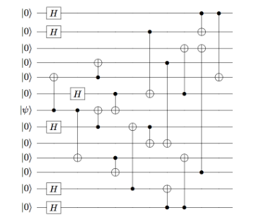
The KQ of a circuit is the number of qubits times the circuit depth, giving an estimate of the number of opportunities for errors to occur [153]. Note that those circuits are not required to be fault-tolerant because the state being purified is generic, rather than inreplaceable data. If the fidelity of the encoded Bell pair is not good enough (e.g. as determined operationally using quantum state tomography), entanglement purification is performed [19, 95].
5.3 Three Methods to Prepare a Heterogeneously Encoded High Fidelity Bell Pair
Entanglement purification is performed to establish high fidelity entanglement [52, 54]. Entanglement purification can be viewed as a distributed procedure for testing a proposition about a distributed state [169].

Figure 5.8 shows the circuit for the basic form of entanglement purification where is a noisy Bell pair. The input is two low fidelity Bell pairs and on success the output is a Bell pair of higher fidelity. One round of purification suppresses one type of error, X or Z. If the initial Bell pairs are Werner states, or approximately Werner states, then to suppress both types, two rounds of purification are required. The first round makes the resulting state into a binary state with only one significant error term but not a significantly improved fidelity. The second round then strongly suppresses errors if the gate error rate is small. Thus, the overall fidelity tends to improve in a stair step fashion. After two rounds of purification, the distilled fidelity will be, in the absence of local gate error,
| (5.1) |
where the original state is the Werner state
| (5.2) |
and is the fidelity if is the desired state. The probability of success of a round of purification is
| (5.3) |
Table B.2 in the appendix provides the numerical data for this to compare with our protocols. Our simulation assumptions are detailed in section 7.3.
5.3.1 Purification before encoding
Figure 5.10 shows the overview of the scheme to make heterogeneously encoded Bell pairs that are purified before encoding. To create an encoded Bell pair of high fidelity, entanglement purification is repeated the desired number of times. Next, each qubit of the purified Bell pair is encoded to its respective error correcting code. To estimate the rate of logical error after encoding, we perform a perfect syndrome extraction of the system to remove any residual correctable errors. After the whole procedure finishes, we check whether logical errors exist. Table B.4 in the appendix presents the details of the simulated error probability and resource efficiency of purification before encoding.
5.3.2 Purification after encoding
Figure 5.12 shows the overview of the scheme to make heterogeneously encoded Bell pairs that are purified after encoding. In this scheme, to create an encoded Bell pair of high fidelity, heterogeneously encoded Bell pairs are generated first by encoding each qubit of a raw physical Bell pair to our chosen heterogeneous error correcting codes. Next, those encoded Bell pairs are purified at the logical level the desired number of times, via transversal CNOTs and logical measurements. Logical purification is also achieved by the circuit shown in Figure 5.8, operating on logical rather than physical qubits. Table B.6 presents the details of the simulated error probability and resource efficiency of purification after encoding.
5.3.3 Purification after encoding with strict post-selection
Figure 5.14 shows the overview of the scheme to make encoded Bell pairs, purified after encoding with strict post-selection protocols to detect errors. This scheme uses a procedure similar to purification after encoding. In this scheme, to create an encoded Bell pair of high fidelity, heterogeneously encoded Bell pairs are generated first by encoding each qubit of a raw physical Bell pair to our chosen heterogeneous error correcting codes. We then run purification protocols at the logical level, similarly to the previous protocol. However, when we perform a logical measurement as part of this protocol, we also calculate (classically) the eigenvalues of all code stabilizers. If any of these eigenvalues are found to be negative, we treat the operation as a failure (in a similar manner to odd parity logical measurements for the purification) and the output Bell pair of the purification is discarded. This simultaneously performs purification and error correction using the properties of the codes. Table B.8 presents the details of the numerically calculated error probability and resource efficiency of purification after encoding with strict post-selection.
5.4 Summary
In this Chapter I proposed three schemes to create heterogeneously encoded Bell pairs between arbitrary two components with scalability. The architecture employs a method that physical Bell pairs are distributed by optical connections and each half of a Bell pair is encoded into heterogeneous quantum error correcting code at distributed components. This method suffers from state errors caused at creation of physical Bell pairs and at the non-fault-tolerant encoding.
To manage such state errors, I propose three schemes to make the method fault-tolerant, Purification before encoding, Purification after encoding and Purification after encoding with strict post-selection.
In Section 7.3, I give the numerical analysis of those error management schemes.
Chapter 6 Scalable distributed QC architecture utilizing benefits of various codes
This chapter proposes the quantum computer architecture for “distributed quantum computing utilizing multiple codes on imperfect hardware”. The most basic requirements to achieve quantum computation in theory are
- •
a quantum universal gate set, and
- •
system size large enough to run quantum algorithms of practical size.
However, physical qubits have error rates higher than we can tolerate, hence
- •
fault-tolerance
is also required. Quantum error correcting codes which achieve the fault-tolerance require excessive resource consumption and have limited ability to achieve a quantum universal gate set. To realize a quantum universal gate set within the limited abilities, more resources are required. See Chap. 1 and 2 for details of those three elements.
This chapter organizes those problems and requirements for the quantum computer architecture and proposes a quantum computer architecture, starting from the fault-tolerance, then the universal gate set and lastly addressing adequate system size.
6.1 Requirements and means to achieve quantum computation
This section discusses why a distributed quantum computer based on the surface code is preferred, and the requirements and means to achieve it.
6.1.1 For fault tolerance
Qubits everywhere always suffer from the quantum imperfections discussed in Section 2.2. The best solution to the quantum imperfections would be to improve the quantum engineering technology. The required error rate to successfully complete a large scale quantum computation properly is , however, the physical state error rate today is around [31]. Therefore, this solution is impractically far away.
The second solution to the quantum imperfections is fault-tolerant quantum computation executed everywhere we use quantum information in the computer. From the point of view of physical feasibility, the surface code is the most promising quantum error correcting code. As stated in Subsec. 2.2.3, the surface code has the highest threshold of physical state error rate in quantum error correcting codes found so far. It requires interactions only between nearest neighbor qubits on a 2-D lattice and is robust against dynamic loss. The surface code is robust against static loss, as shown in Chap. 3.
Therefore the proposed architecture employs the surface code as the fundamental quantum error correcting code.
6.1.2 For universal quantum computation
A universal quantum computer requires a universal set of quantum gates. As noted in Subsec. 2.1.5, by Solovay-Kitaev decomposition, the set of the gate, gate and gate is a universal set. No quantum error correcting code which is practically feasible in 2-D fashion and which produces a universal gate set has been discovered [15].
As shown in Subsec. 2.2.3, since the surface code does not support the gate in a transversal, fault-tolerant fashion, the surface code requires an ancilla-supported gate utilizing an state. The ancilla-supported gate problematically requires the application of an gate as a correction and the surface code also does not support gate in a transversal, fault-tolerant manner, hence the surface code needs the ancilla-supported gate utilizing a state, too.
There are several ways to generate the ancilla states and in the surface code. The first way is state injection from physical qubits followed by the magic state distillation [19, 21]. Though the magic state distillation guarantees adequate fidelity of injected and , its process is stochastic and its cost is high both in space and in time. To achieve a stable supply of the ancilla states generated probabilistically and to distribute the required number of ancilla states which are generated in groups in a magic state distillation [21] to the required locations, division of components used to generate ancilla states from components used to execute quantum gates would be preferred.
The second way is to get support from other error correcting codes by code teleportation (conversion) [25, 36]. The Reed-Muller code can create transversally. The Steane [[7,1,3]] code can create transversally. As stated in [36], this approach is advantageous only when the concatenation level of supporting codes is low and when the cost of magic state injection and distillation is relatively expensive. Such complementary code may prefer a different physical architecture, such as physical qubit layout, from the surface code, hence separated components for the complementary code from those for the surface code is preferred.
Either way may prefer separated components to generate ancilla states from those for the surface code. Therefore the proposed architecture employs separate, dedicated components to generate ancilla states, leaving the selection flexible.
6.1.3 For system size large enough
As mentioned in Chap. 1, Shor’s algorithm to factor a number described with bits requires at least high-quality qubits. Additionally, as noted in Subsec. 2.2.3 and 6.1.1, the surface code requires excessive resource overhead. Installing all quantum computational resource on a single quantum chip would not be feasible, as noted in Chap. 1. Hence, to execute quantum algorithms to solve practically meaningful large problems, we need to connect components of small performance to build up a large scale quantum computer.
Connecting many components leads to the idea of division of roles among components [130, 39]. The roles in computation are broadly divided into logic operations and storage. By dividing roles, we can combine the two benefits, executing quantum operations in fast fashion in quantum CPUs and storing quantum information in space-saving fashion in quantum memories. Therefore, different choices may be made in different components, such as choice of physical technologies [31] and error correcting codes [39, 25]. Unlike the CPUs of the conventional computer of today, quantum logic gates are not relatively high-level instructions [111, 165, 180]. Quantum CPUs with the surface code are more like executing logic gates directly on memory than integration of registers, pipelined devices, ALUs and so on [87, 172, 45]. Hence the first difference of quantum CPUs and quantum memories is the choice of quantum error correcting code. The physical implementation of the components will vary depending on the quantum error correcting code; this dissertation leaves physical technologies employed by each component flexible. Different quantum error correcting codes have different duration for quantum logic gates and different resource consumption. Therefore the proposed architecture employs the defect-based surface code in quantum CPUs and employs the deformation-based surface code in quantum memories.
Connecting components requires internal quantum connections in a quantum computer. Such connections must support heterogeneous encoding and must be fault-tolerant. Oskin et al. and Copsey et al. proposed architectures utilizing code teleportation based on heterogeneously encoded Bell pairs [130, 39]. Their means are not robust against errors during encoding. Monroe et al. and Ahsan et al. proposed an internal connection backplane utilizing optical crossbar switches for scalability of parallelism of connections [114, 1]. Extending their means to involve purification, discussed in Chap. 5, this system realizes a scalably fault-tolerant interconnection supporting heterogeneous encoding. Components need to support quantum teleportation using the Bell pairs shared by the backplane.
6.2 Requirements of building blocks and internal connections of the proposed architecture
In my design, the roles for quantum computation are divided to three types of building blocks and a backplane, the internal connections of building blocks. The three types of building blocks are quantum CPUs which execute quantum algorithms, quantum memories which maintain quantum data that is not operated at that time, and magic state generation areas which produce magic states for non-Clifford gates.
Table 6.2 summarizes the must-have requirements of building blocks of the quantum computer architecture for “name will be added”. Other desirable but less critical features are discussed in the following section.
The requirements for quantum CPUs can be summarized as processing quantum data without any problems. Therefore, quantum CPUs must tolerate quantum imperfections; they must support a universal gate set; and they must support transferring quantum data to and from the internal connection point.
The requirements for quantum memories can be summarized as maintaining quantum data without any problems. Therefore, quantum memories must tolerate quantum imperfections; and they must support transferring quantum data to and from the internal connection point.
The requirements for magic state generation area can be summarized as producing high fidelity magic states for non-Clifford gates. Hence, magic state generation areas must tolerate quantum imperfections; they must create magic states of high fidelity, such as and ; and they must support transferring quantum data to and from the internal connection point.
The requirements for internal connections can be summarized as transfer quantum data from one building block to another with adequate fidelity. Hence, internal connections must tolerate quantum imperfections; they must support routing of data transfer; and they must bridge heterogeneous error correcting codes.
| element | requirements |
|---|---|
| Quantum CPUs | tolerate quantum imperfections |
| support an universal gate set | |
| support transferring quantum data | |
| Quantum Memories | tolerate quantum imperfections |
| support transferring quantum data | |
| Magic State | tolerate quantum imperfections |
| Generation | create magic states of high fidelity, such as and |
| area | support transferring quantum data |
| Internal connections | tolerate quantum imperfections |
| support routing of data transfer | |
| bridge heterogeneous error correcting codes |
6.2.1 Desired characteristics of building blocks and internal connections
For the division of roles, building blocks and internal connections have different desirable characteristics. Table 6.4 summarizes the desired characteristics of building blocks and internal connections.
Quantum CPUs desire fast quantum gates to minimize computation time. When employing fast gates, high consumption of spatial resources would be an acceptable compromise as long as the quantum memories are spatially efficient so that the overall system size is feasible.
Quantum memories desire spatially small resource requirement to minimize the overall system size. As long as quantum CPUs have fast gates to process the quantum computation rapidly, slow operations on quantum memories would be an acceptable compromise; by analogy with classical computers, access time to memories that is hundreds of times slower than registers in CPU would be acceptable [71].
For the magic state generation area, as noted in Subsec. 6.1.2, there are two candidates for the design and the better design differs depending on the environment and on the performance of base technologies. This area should employ the design which prepares ancilla states more efficiently in terms of the product of space and time, when building the quantum computer. I leave the design of this area flexible.
Internal connections hopefully have scalable parallelism of connections. With scalable parallelism of connections, stall of computation caused by queued data transfer would be reduced.
| element | desired characteristics |
|---|---|
| Quantum CPUs | fast gates |
| Quantum Memories | space-saving design |
| Magic State | space-saving design |
| Generation | fast preparation of magic states |
| area | |
| Internal connections | scalable data transfer |
6.3 The proposed quantum computer architecture

Figure 6.2 shows the proposed quantum bus architecture, extended from [1, 91]. Colored lines are optical connections or internal photon path of the optical crossbar. The red lines are inputs to the crossbar switch. The blue lines are outputs from the crossbar switch. Each input source component has links with the crossbar and holds a solid qubit to emit a photon. Two output lines lead to a Bell state analyzer (BSA), which executes Bell measurement for entanglement swapping [77].
To achieve quantum communication between two components, each of the two components emit a photon to the crossbar switch so that we have each stationary qubit entangled with a photon, leaving a solid qubit behind in the component. The crossbar switch switches the connections to route the two photons to two links to an assigned BSA. BSA executes Bell measurement on the two photons for entanglement swapping, leaving the two stationary qubits in the two components entangled.
Each of the two solid qubits is then encoded to the error correcting code used in the component. This homo- or hetero-encoded Bell pair is created as the resource for quantum teleportation at the logical level.
The deformation-based surface code area and the defect-based surface code area work as quantum memories and as CPUs, respectively. Their physical implementation may be same. Both of them have physical qubits placed on a 2-D lattice, since the surface code runs in both area. However, the encoding of logical qubits on the surface code lattice differs, therefore the way of using the devices differs depending only on software.
6.3.1 Defect-based surface code area
This area employs the defect-based surface code [62]. the gate by braiding requires steps, for steps for each of first half expansion, first half shrink, second half expansion and second half shrink respectively.
6.3.2 Densely packed deformation-based surface code area
This area employs the deformation-based surface code proposed in Chapter 4. The deformation-based surface code packs logical qubits denser than other surface codes. Logical and logical can be executed efficiently. However, logical gate by lattice surgery requires steps where is the code distance while steps are required for the standard planar code. This fact would make the deformation-based surface code area hundreds of times slower than the defect-based code area. On top of this, the logical Hadamard gate of the deformation-based qubit is three times slower. Hence this area should be a storage, or a memory, to keep logical qubits for a long time in a spatially efficient fashion. A concern is whether the hundreds slower memory than the CPU is usable or not. In my design, the memory access time is proportional to the duration of gate because data transfers are implemented by quantum teleportation. I would conclude that the much slower memory is acceptable from this fact in classical computers [71].
gate for the deformation-based surface code is expensive, hence teleportation based on stabilizer is more preferred to send a logical qubit from this memory. Such as, the first state is
| (6.1) |
where qubit is the state we want to send and qubits and are a Bell pair and qubit is an ancilla qubit for the stabilizer. By applying and , we get
| (6.2) |
by measuring and applying if eigenvalue is observed, then we get
| (6.3) |
by measuring and and applying for each measurement if eigenvalue is observed, then eventually we get
| (6.4) |
6.3.3 Magic state generation area
This area may consist of quantum chips of several codes, such as the Steane [[7,1,3]] code and the Reed-Muller 15 qubit code. This is because the Steane [[7,1,3]] code can create an ancilla state for an S gate efficiently and the Reed-Muller 15 qubit code can create an ancilla state for a T gate efficiently [85].
Another possible implementation is of the surface code, to create logical ancilla states by magic state distillation [19, 63]. It is not yet sure which is better for this purpose the defect-based code with braiding of the planar code with lattice surgery.
Created ancilla states are sent to the computation areas by quantum teleportation. With any codes, the chip must have dedicated design for distillation.
6.3.4 Network interface card
The network interface card has one or more attachments for optical fibers to connect to other quantum nodes, after the classical network interface card. By utilizing this component, the computation chips are enabled to cooperate with computation chips installed in other machines.
External links have much larger loss/error rate than internal links because of the environment and the longer fiber [81]. External links can achieve Bell pair creation at a lower rate than internal links do, hence internal Bell pairs may go unused as we wait for an external Bell pair. Figure 6.2 has only one network interface card and only one external link from the card. If more throughput is required, we can employ a network interface card which has two or more fiber attachments instead and use two or more fibers for the link. The new fiber should be connected to the same repeater/router as the first one, then the quantum links are aggregated after the classical link aggregation [79].
Another means to increase throughput is inserting another network interface card. This means allows the quantum computer to be connected to two quantum repeaters/routers/computers. This may be useful for complex use of quantum network. This work targets the bus architecture and more consideration about network interface cards is an open problem.
6.4 Hardware and Software of building blocks
Both quantum CPUs and quantum memories employ the surface code, so their physical implementation are the same; they have 2-D lattice of physical qubits in which nearest neighbor interactions are implemented; and on the edges of the components, optical-solid conversion is implemented for internal connections. Therefore the difference of the two areas will be how the physical qubits are used by software; how logical qubits are encoded; how logical gates are executed; and how logical qubits are transferred.
If magic state generation area employs the surface code with state injection and magic state distillation, its hardware implementation will be same as the quantum CPUs and quantum memories. Then, the software may be the same as the quantum CPUs. If it employs the other, the hardware implementation will depend on the employed error correcting code.
The hardware of internal connections are composed from optical fibers, the optical cross bar switch and BSAs. The number of optical fibers connected to a component directly affects the performance of the bandwidth of the internal communication. One BSA can support one internal connection at a time. Hence the parallelism of internal connections is determined by the number of BSAs [1, 91].
Chapter 7 Evaluation
7.1 Performance of the surface code on defective lattice
We assume a circuit-based error model, summarized by Landahl et al. [104]. This circuit-based error model assumes that each gate acts ideally, followed by a noisy channel, and that each measurement acts ideally, after a noisy channel. Errors may occur at every gate in the circuit. Our error channel for a single-qubit gate has error probability , meaning that each error (X, Z or Y) occurs with probability /3. In a similar fashion, for two-qubit gates, our error model has probability /15 for each two-qubit error (IX, IZ, IY, XI, XX, XZ, XY, ZI, ZX, ZZ, ZY, YI, YX, YZ, YY). We assume that the set of physical gates available includes CNOT, SWAP and Hadamard gates. We assume that INIT and measurement in Z basis have X error probability . All operations require one time step.
Our circuit is asynchronous in the sense that stabilizers are measured at different frequencies. Stabilizers whose circuits have shallower depth may be measured more times than those whose circuits have deeper depth. To achieve proper syndrome matching, the surface code requires that the lattice be covered by stabilizers. Otherwise, an unstabilized area works as a defect-based qubit which may serve as an end of error chains, leading to undetectable logical errors. Hence, after all stabilizers covering the lattice have been measured at least once since the last execution of the matching algorithm, the matching algorithm is re-executed. Typically, this timing is dependent on the deepest stabilizer circuit. From the result of matching, we make a map of Pauli frames which describes where Pauli frame corrections should be applied for error correction. Because our circuit is asynchronous and there might be SWAP gates, we must keep track of the location of data qubits to combine the error information about data qubits and the map to check the result of error correction.
We have conducted extensive simulations, beginning with a perfect lattice, then extending to imperfect ones. First we show the numerical result of several basic test cases: only a single faulty device exists, in the center of the lattice; only a single faulty device exists, in the west of the lattice; and only a single faulty device exists, in the northwest of the lattice for the distances 5, 7, 9 and 13. Our simulation holds temporal rounds of measured stabilizer values for error correction. Hence measurements are saved for the stabilizer with the deepest circuit and more measurements are saved for normal stabilizers, because of the scheduling algorithm shown in Subsection 3.3. After finishing an error correction cycle, the oldest round is discarded, a new round is created by new measurements and error correction is re-executed. Next, we show the numerical result for random generated lattices for different yields, 80%, 90% and 95%. We generated 30 lattices for each pair of yield and code distance of 5, 7, 9, 13, 17 and 21. Some defective lattices cannot encode a logical qubit for the code distance becomes 0 as a result of merging stabilizers, so that eventually we simulate 478 lattices (details described in subsection 7.1.3) for each physical error rates of , , , , , , , , , and . It is hard to collect enough logical errors in Monte Carlo simulation as the logical error rate is exponentially suppressed, therefore we choose as the lowest physical error rate for our simulation. Therefore we simulated 5258 parameter combinations.
The computational resource devoted to circuit simulation, excluding chip generations and circuit constructions, was more than 100,000 CPU days, executed on the StarBED project testbed [112]. Each preparation of stabilizer circuits which solves the traveling salesman problem required up to 1 CPU day. After construction of the nest, for example, the simulation of of single-faulty-northwest for consisted of 370945 rounds of error correction to find 500 logical errors in 1424.98 seconds. The simulation of of single-faulty-northwest for consisted of 315550 rounds of error correction in 5.8 days but found 0 logical errors.
Peak memory sizes are estimated to be 30GB for 320 lattices, 63GB for 133 lattices and more than 100GB for 25 lattices. The greatest memory consumption is during nest building, shown in Figure B5, B6 and B7. To give accurate weights to the edges of the “nests”, Autotune virtually creates errors on every qubit at every physical step, and traces their propagation. Roughly speaking, the size of the error structure is 136 bytes. A lattice includes 1089 qubits for distance 17. Let us assume: 200 physical steps per error correction cycle due to the asynchronous stabilizers; each error propagates to 10 physical qubits on average; each error remains for 100 physical steps on average. Then memory consumption is bytes, roughly 30 GB. Several factors affect this rough estimate. Faulty devices reduce the number of qubits and other structures generated to create the nests, but the memory consumption remains on the order of tens giga bytes.
Those peak memory sizes are big, however, they do not affect the quantum computation in practice. This is because the heavy operations that Autotune virtually creates errors on every qubit at every physical step, and traces their propagation by the circuits to give accurate weights to the edges of the nests can be executed preliminarily. To avoid redundant execution of heavy creation of nests, all 11 physical gate error rates for a single lattice are simulated in parallel on a single simulation node, allowing us to share a single in-memory copy of the nest. We attempted to simulate distance 21, but failed because we cannot accumulate enough logical errors to have valid data points, for one of several reasons: good lattices have strong tolerance against errors; even bad lattices have strong error tolerance at lower physical error rate; at higher physical error rates, simulating an error correction cycle takes too much computation time because many physical errors occur in our extended asynchronous error correction cycle, taxing the scalability of the matching algorithm; or because the simulation requires more than 128GB memory, the maximum available in our system.
7.1.1 perfect lattice
Figure 7.2 depicts the results of simulation of perfect lattices, used as our baseline for comparison. Each curve represents a set of simulations for a lattice of a particular code distance, for varying physical gate error rates. Points below the break-even line are conditions in which the logical error rate in the logical state is below that of a bare, unencoded physical qubit. The break-even line indicates whether the error correcting code bears fruit at the physical error rate in the sense of the error probability, with lengthening the execution time of the quantum computation since a logical gate consists of many physical gates. Distance 9 achieves break-even at . The crossing point of the curves, each of which describes a code distance, is called the threshold, the physical error rate below which the larger code distance has the lower logical error rate. Above the threshold, the error correction process introduces more errors than it corrects, and the higher code distance has the higher logical error rate.
The threshold indicated by this simulation is around , similar to the reported in [63]. This related work employs the assumptions most similar to our perfect lattice simulation, other than the asynchronous scheduling of stabilizers. Our error correction circuits are designed to omit identity gates to shrink the asynchronous circuit depth, whereas circuits of related work achieve perfect synchronization and parallelism through careful insertion of identity gates. For example, identity gates on the qubit d17 in Fig 2.12 (b) between the initialization and the CNOT gates or between the CNOT gates and the measurement are omitted in our simulation. We infer that our baseline simulation follows the related work, our baseline simulation is valid and the effect of asynchronicity to the perfect lattice is small.

7.1.2 lattice with a single faulty device
Figure 7.4(a), (b) and (c) depict the results of simulations to investigate the effect of a single faulty device in the center, on the west edge and on the northwest corner of the lattice, respectively. The plots show that our approach works properly because the larger code distance has the lower logical error rate at lower physical error rates.
(a)

(b)

(c)

Each single-fault residual error rate is worse than that of the corresponding perfect lattice. The slope of each code distance of single-fault chips is lower than that of the corresponding perfect lattice. The gap grows slightly as the physical error rate is reduced, visible as the less-steep curve for the defective lattice.
There are differences depending on the single-fault location. Comparing the points of the perfect lattice with those of single-faulty-center, single-faulty-west and single-faulty-northwest at , faulty lattices are , and worse than the perfect lattice, respectively. Single-faulty-northwest has a lower residual error rate than the others. This may be because the big stabilizer which causes asynchronous scheduling of stabilizers is on the periphery, so that the number of stabilizers which are close to the big stabilizer and hence which have stronger scheduling restrictions than more remote stabilizers is smaller than other single-faulty chips. Across the range of our simulations, the negative impact is depending on location, distance and error rate.
From the point of view of absolute logical error rate, the penalty for having a defect is greater at lower physical error rates. An “effective” code distance is the code distance at the same physical error rate of the perfect lattice which has the closest logical error rate to the defective lattices. For single-faulty-center, at , faulty is worse than perfect , hence the effective code distance of faulty at is . The effective code distance is useful when considering the resource overhead of modifications. In the example above, to achieve a logical error rate equivalent to that of on the perfect lattice at , we at least need for the defective lattice. This indicates that the number of physical qubits are required.
From the point of view of the effective code distance, the penalty for having a defect is smaller at lower physical error rates. At , faulty is worse than perfect , and at , faulty is better than perfect while faulty is worse than perfect . Hence, to exceed the effective code distance 5, requires us to use while only requires us to use . The trend of the penalty of the effective code distance and that of the absolute logical error rate differ. This difference is caused by the difference of slopes of each code distance of each lattice. We have to be mindful of those trends when designing a quantum computer to achieve an adequate logical error rate.
Because the proportional impact of a single fault should lessen as the code distance increases, the crossing point of the curves is not a good measure of performance here. Figure 7.4 shows that the crossing points of two distances would differ. The crossing point of distance 9 and 13 appears to be around which is the threshold for the perfect lattice as shown in Figure 7.2, whereas the crossing point of distance 5 and 7 is around .
Table 7.2 shows the data of the single-faulty lattice simulations. The reduced code distance is the minimum distance between corresponding boundaries shortened by merging stabilizers. The naive hypothesis would be that reduced code distance is a good metric to predict the logical error rate of the lattice, since the number of physical errors required to cause a logical error is a minimum on the shortest logical operator, which is the minimum distance between corresponding boundaries. However, the effect is more complex. We will explore this further in Section 7.1.3 and Chapter 8.
| faulty | code | #X and | residual | reduced | #Z stabs | biggest | steps per | ave. | biggest | ave. steps | ave. #dataq |
| location | distance | Z | X error | distance | #dataq | error | of Z | Z | per error | of Z stabs | |
| stabs | rate | of Z | correction | stabs | correction | ||||||
| stabs | cycle | of Z stabs | |||||||||
| center | 5 | 38 | 7.038E-02 | 4 | 19 | 6 | 32 | 35.871 | 195.194 | 8.844 | 3.684 |
| west | 5 | 38 | 6.843E-02 | 4 | 19 | 6 | 32 | 35.803 | 195.194 | 8.822 | 3.684 |
| northwest | 5 | 38 | 3.335E-02 | 4 | 19 | 6 | 32 | 35.648 | 195.194 | 8.791 | 3.684 |
| center | 7 | 82 | 3.704E-02 | 6 | 41 | 6 | 32 | 32.249 | 195.194 | 8.149 | 3.756 |
| west | 7 | 82 | 3.319E-02 | 6 | 41 | 6 | 32 | 32.270 | 195.194 | 8.153 | 3.756 |
| northwest | 7 | 82 | 1.969E-02 | 6 | 41 | 6 | 32 | 32.505 | 195.194 | 8.228 | 3.756 |
| center | 9 | 142 | 2.224E-02 | 8 | 71 | 6 | 32 | 31.215 | 195.194 | 7.943 | 3.803 |
| west | 9 | 142 | 1.873E-02 | 8 | 71 | 6 | 32 | 31.456 | 195.194 | 8.016 | 3.803 |
| northwest | 9 | 142 | 1.046E-02 | 8 | 71 | 6 | 32 | 31.539 | 195.194 | 8.033 | 3.803 |
| center | 13 | 310 | 8.776E-03 | 12 | 155 | 6 | 32 | 30.711 | 195.194 | 7.824 | 3.858 |
| west | 13 | 310 | 8.662E-03 | 12 | 155 | 6 | 32 | 31.028 | 195.194 | 7.910 | 3.858 |
| northwest | 13 | 310 | 4.869E-03 | 12 | 155 | 6 | 32 | 31.084 | 195.194 | 7.925 | 3.858 |
7.1.3 Random multiple faulty devices
We generated 30 randomly defective lattices for each combination of three yields, , and and of 5 code distances, 5, 7, 9, 13, 17, so that we generated 450 lattices. Table 7.4 shows the number of defective lattices generated and simulated. On some defective lattices, by chance the faulty qubit placement results in a lattice for which we are unable to build an effective circuit for encoding a logical qubit, so they are not simulated. Our software successfully built circuits for almost all lattices at and above, but only about two-thirds at .
| yield | 0.80 | 0.90 | 0.95 | ||||||||||||
|---|---|---|---|---|---|---|---|---|---|---|---|---|---|---|---|
| code distance | 5 | 7 | 9 | 13 | 17 | 5 | 7 | 9 | 13 | 17 | 5 | 7 | 9 | 13 | 17 |
| #encodable | 20 | 24 | 22 | 19 | 19 | 29 | 29 | 30 | 30 | 30 | 28 | 30 | 30 | 30 | 30 |
| #unencodable | 10 | 6 | 8 | 11 | 11 | 1 | 1 | 0 | 0 | 0 | 2 | 0 | 0 | 0 | 0 |
| y | 0.80 | 0.90 | 0.95 | ||||||||||||
|---|---|---|---|---|---|---|---|---|---|---|---|---|---|---|---|
| d | 5 | 7 | 9 | 13 | 17 | 5 | 7 | 9 | 13 | 17 | 5 | 7 | 9 | 13 | 17 |
| all | 13.9 | 29.7 | 54.0 | 122.6 | 215.6 | 8.4 | 16.2 | 29.6 | 61.0 | 107.3 | 3.8 | 8.0 | 14.7 | 31.3 | 53.7 |
| 50% | 13.2 | 28.9 | 55.1 | 122.6 | 214.5 | 7.3 | 14.2 | 26.7 | 56.3 | 101.7 | 2.9 | 7.1 | 11.9 | 28.5 | 51.3 |
| 90% | 12.3 | 29.0 | 55.0 | 121.3 | 221.7 | 5.7 | 9.3 | 23.7 | 48.0 | 96.0 | 1.7 | 4.7 | 9.0 | 25.3 | 51.3 |
This unencodable condition occurs when a defective data qubit chain stretches from a boundary of the lattice to the other boundary of the same type (south and north for Z stabilizer boundary, or west and east for X stabilizer boundary). For instance, if a faulty qubit is on a boundary, say, the which is stabilized by of the stabilizer and the qubit is not stabilized by another Z stabilizer, then cannot be merged with another stabilizer to work around . Hence we remove with and eventually , and become a part of the boundary instead. In general, this adaptation reduces the code distance (shown in Tables 7.8 and 7.10). Therefore, a lattice of lower yield and of lower code distance may be unencodable with higher probability. Though only 30 instances for each condition are too few to get explicit statistics, table 7.4 shows this trend at yields of 90% and 95%. might be saturated in encodable rates because the code distances do not show meaningful differences.
Figure 7.6 shows the geometric mean of sets of encodable lattices, plotting physical error rates versus logical error rates. Appendix A.2 shows the scatter plots of raw data.


The left column in Figure 7.6 show the graphs of , describing the geometric mean of all encodable lattices, of the better 50%, and of the best 10% of generated lattices, from the top, respectively. Note that those cull percentages are based on the original set of 30 generated lattices, not the smaller number of the encodable lattices. Some points of longer distance at lower physical error rate are not plotted since not enough logical errors are accumulated because of the very low logical error rates.
At functional qubit yield, we see many chips beating break-even at . The threshold is about , about half of the threshold error rate for a perfect lattice. The significant penalty in both threshold and residual error rate can be dramatically reduced by culling poorer chips and discarding them. At cull at , the residual error rate for is about that of with a perfect lattice, and is about that of a perfect .
Naturally, the logical error rates get better as we discard more of the poorest lattices. At , unculled shows that even distance 17 is just on the break-even line and 90%-culled (c) shows that all 5 distances exceed break-even. The steepness of the slope of the curves of culled defective lattices exceeds that of the curves of lower code distances on the perfect lattice, though it does not match the perfect lattice of the same distance. Thus, an appropriate culling strategy reduces the penalty for a 5% fault rate to a manageable level, allowing us to achieve a desired level of error suppression by using a slightly larger code distance. At , by culling , the penalty against the perfect lattices changes from to at , from to at , and from to at . We do not have data points for -culled of and of since not enough logical errors are accumulated on their best of the lattices. The smaller code distance gets closer to the perfect lattice because it has fewer qubits, therefore good outliers may be generated with higher probability, as shown in Table 7.6. Table 7.6 summarizes the average number of static losses on all the generated lattices, on the 50%-culled lattices and on the 90%-culled lattices. The remaining 3 lattices of 90%-culled distance 5 have 1, 2 and 2 static losses respectively. Table 7.6 also allows us to see that the importance of static loss placement because the numbers of static losses of longer distances do not decrease much but all the logical error rates gets better.
The middle column in Figure 7.6 is the graphs of , under the same conditions with those of . The threshold is about , about a quarter of the threshold for a perfect lattice. At cull (in the middle-bottom of Figure 7.6), at , the residual error rates for , and are about twice those of with a perfect lattice. would be better than that of perfect , but it is missing since the logical error rate may be too low to accumulate enough number of logical errors. At of , unculled (middle-top) shows that only distance 13 exceeds the break-even, but 90%-cull (middle-bottom) shows all five distances exceed the break-even.
The right column in Figure 7.6 is the graphs of . At , we have already seen that only two-thirds of the chips can even be encoded. Our simulations indicate that even those chips for which we could create a circuit are unusable. Even at , there is no evidence of a correctable threshold, and although residual error rates do decline as the physical error rate is reduced, only a single data point reaches break-even. We conclude that is not good enough to build a computer.
Unculled shows that distances 13 and 17 are approximately identical at , while other distances show that longer is better. Unculled distance 13 and 17 for do not show that longer is better, though other distances do. Unculled shows that distance 7 exceeds distance 5 at , while other distances do not show an improvement for the longer distance. Those indicate that the longer code distances cross at lower physical error rate. We need to consider this fact when deciding the code distance to use.
7.1.4 Metrics for selecting good chips
Both to improve our understanding of the root causes of the error rate penalty and to provide a simple means of selecting good chips, we evaluated the correlation between a set of easy-to-calculate metrics and the simulated residual error rate. Tables 7.8 and 7.10 describe the correlations between eighteen metrics and logical error rates or log(logical error rates), respectively, for for each combination of yield and code distance.
The simplest possible metrics, just counting numbers of qubits in various categories, show only modest correlation.
Steane’s metric is the space-time product of a circuit: the number of qubits involved, multiplied by the circuit depth [156].
The and is the product of the “cycle”, which is the average number of steps in a stabilizer measurement and the number of data qubits or the total number of qubits including ancillae involved in the stabilizer, respectively. The and reflect the total probabilities of possible physical errors which occur in a measurement of the stabilizer. Both Tables 7.8 and 7.10 indicate that the average of the and the average of the of stabilizers have the strongest and the second strongest correlations with the logical error rate. The average number of qubits in a stabilizer and the average “cycle” of stabilizers show the next strongest correlations. Those mean that the accumulation of possible errors in a stabilizer may be the factor most strongly correlated to the logical error rate.
Somewhat to our surprise, both the of the largest stabilizer and the average across the entire lattice do not have good correlations. This may be because this form of does not correctly capture the total probabilities of possible physical errors which occur in a measurement of the stabilizer.
Table 7.6 implies that the number of faulty devices is correlated with the logical error rate. By culling bad lattices, Table 7.6 shows that the average number of faulty devices on a lattice is reduced and Figure 7.6 shows that the logical error rate gets better. However, the average of stabilizers has significantly higher correlation with logical error rate, 0.76, than that of the number of faulty devices, 0.43. We calculated the cross-correlation of elements for and . The correlation between the number of faulty devices and the average of stabilizers is 0.79.
The number of faulty ancilla qubits is the most weakly correlated to the logical error rate. This fact indicates that even if the number of faulty ancilla qubit increases, the logical error rate does not decline rapidly. For a given yield, the placement of faults matters more than the exact number.
| yield | code | #stab | #flty | #flty | #flty | # | bgst | ave. | bgst | ave. | dpst | ave. | bgst | ave. | bgst | ave. | bgst | ave. | bgst | ave. | bgst | ave. | ave. | |
| dist. | qubit | data | syn. | redu- | stab | #qubit | #qubit | #data | #data | depth | depth | # | ||||||||||||
| qubit | qubit | ced | of | of | qubit | qubit | of | of | of | of | of | of | cycle | cycle | of | of | of | of | stab | |||||
| dist. | stabs | stabs | of | of | stabs | stabs | msmts | |||||||||||||||||
| stabs | stabs | stabs | stabs | stabs | stabs | stabs | stabs | stabs | stabs | /step | ||||||||||||||
| 0.95 | 5 | -0.64 | 0.59 | 0.70 | 0.08 | -0.67 | -0.71 | 0.81 | 0.83 | 0.79 | 0.71 | 0.26 | -0.01 | 0.24 | 0.37 | 0.23 | 0.16 | 0.69 | 0.71 | 0.74 | 0.88 | 0.76 | 0.86 | -0.69 |
| 0.95 | 7 | -0.40 | 0.45 | 0.65 | -0.13 | -0.62 | -0.46 | 0.65 | 0.44 | 0.70 | 0.44 | 0.05 | 0.00 | 0.07 | 0.11 | 0.08 | 0.04 | 0.78 | 0.55 | 0.76 | 0.78 | 0.79 | 0.79 | -0.44 |
| 0.95 | 9 | -0.50 | 0.68 | 0.72 | 0.33 | -0.60 | -0.48 | 0.63 | 0.81 | 0.64 | 0.79 | 0.42 | -0.07 | 0.46 | 0.48 | 0.40 | 0.24 | 0.62 | 0.81 | 0.67 | 0.88 | 0.68 | 0.89 | -0.69 |
| 0.95 | 13 | -0.28 | 0.48 | 0.55 | 0.11 | -0.19 | -0.27 | 0.36 | 0.56 | 0.37 | 0.52 | -0.02 | -0.47 | 0.02 | -0.14 | 0.03 | -0.25 | 0.30 | 0.59 | 0.33 | 0.71 | 0.34 | 0.69 | -0.40 |
| 0.95 | 17 | -0.18 | 0.34 | 0.27 | 0.25 | -0.10 | -0.18 | 0.20 | 0.39 | 0.15 | 0.40 | 0.05 | -0.32 | 0.17 | -0.06 | 0.05 | -0.16 | 0.13 | 0.50 | 0.11 | 0.56 | 0.10 | 0.55 | -0.40 |
| 0.90 | 5 | -0.19 | 0.35 | 0.26 | 0.29 | -0.48 | -0.24 | 0.62 | 0.20 | 0.55 | 0.16 | -0.23 | -0.21 | 0.06 | -0.13 | -0.11 | -0.16 | 0.49 | 0.28 | 0.69 | 0.48 | 0.62 | 0.46 | -0.21 |
| 0.90 | 7 | -0.31 | 0.37 | 0.43 | 0.07 | -0.59 | -0.33 | 0.50 | 0.53 | 0.49 | 0.45 | 0.20 | -0.33 | 0.59 | 0.23 | 0.43 | -0.01 | 0.51 | 0.58 | 0.71 | 0.71 | 0.70 | 0.74 | -0.46 |
| 0.90 | 9 | -0.39 | 0.40 | 0.54 | 0.09 | -0.65 | -0.42 | 0.67 | 0.65 | 0.63 | 0.58 | -0.29 | -0.54 | 0.01 | -0.12 | -0.18 | -0.32 | 0.28 | 0.39 | 0.43 | 0.68 | 0.43 | 0.66 | -0.45 |
| 0.90 | 13 | -0.36 | 0.47 | 0.63 | -0.01 | -0.30 | -0.37 | 0.47 | 0.77 | 0.52 | 0.81 | -0.26 | -0.25 | -0.10 | 0.24 | -0.28 | 0.04 | 0.46 | 0.57 | 0.60 | 0.81 | 0.62 | 0.81 | -0.51 |
| 0.90 | 17 | -0.55 | 0.58 | 0.62 | 0.10 | -0.62 | -0.56 | 0.56 | 0.76 | 0.56 | 0.74 | -0.05 | -0.25 | 0.34 | 0.33 | 0.10 | 0.08 | 0.17 | 0.65 | 0.35 | 0.86 | 0.37 | 0.87 | -0.74 |
| 0.80 | 5 | -0.20 | 0.30 | 0.22 | 0.17 | -0.43 | -0.22 | 0.78 | 0.59 | 0.46 | 0.40 | -0.11 | -0.13 | 0.43 | 0.30 | -0.19 | 0.05 | 0.64 | 0.72 | 0.78 | 0.75 | 0.63 | 0.67 | -0.49 |
| 0.80 | 7 | 0.22 | 0.35 | 0.10 | 0.40 | -0.51 | 0.13 | 0.56 | 0.81 | 0.44 | 0.75 | 0.07 | -0.34 | 0.29 | 0.58 | 0.03 | 0.24 | 0.56 | 0.74 | 0.64 | 0.79 | 0.69 | 0.83 | -0.48 |
| 0.80 | 9 | -0.39 | 0.37 | 0.31 | 0.15 | -0.47 | -0.38 | 0.63 | 0.88 | 0.68 | 0.68 | -0.42 | -0.45 | 0.41 | 0.58 | 0.12 | -0.01 | 0.50 | 0.77 | 0.58 | 0.86 | 0.66 | 0.92 | -0.53 |
| 0.80 | 13 | 0.02 | 0.34 | 0.18 | 0.20 | -0.43 | -0.05 | 0.65 | 0.79 | 0.66 | 0.80 | 0.21 | 0.09 | 0.45 | 0.68 | 0.22 | 0.52 | 0.70 | 0.63 | 0.65 | 0.79 | 0.70 | 0.84 | -0.35 |
| 0.80 | 17 | 0.39 | 0.25 | 0.19 | 0.19 | -0.24 | 0.34 | 0.37 | 0.60 | 0.29 | 0.57 | -0.15 | -0.41 | 0.28 | 0.37 | 0.04 | 0.07 | 0.51 | 0.55 | 0.34 | 0.61 | 0.33 | 0.62 | 0.16 |
| average | -0.25 | 0.42 | 0.42 | 0.15 | -0.46 | -0.28 | 0.56 | 0.64 | 0.53 | 0.59 | -0.02 | -0.25 | 0.25 | 0.25 | 0.06 | 0.04 | 0.49 | 0.60 | 0.56 | 0.74 | 0.56 | 0.75 | -0.44 | |
| yield | code | #stab | #flty | #flty | #flty | # | bgst | ave. | bgst | ave. | dpst | ave. | bgst | ave. | bgst | ave. | bgst | ave. | bgst | ave. | bgst | ave. | ave. | |
| dist. | qubit | data | syn. | redu- | stab | #qubit | #qubit | #data | #data | depth | depth | # | ||||||||||||
| qubit | qubit | ced | of | of | qubit | qubit | of | of | of | of | of | of | cycle | cycle | of | of | of | of | stab | |||||
| dist. | stabs | stabs | of | of | stabs | stabs | msmts | |||||||||||||||||
| stabs | stabs | stabs | stabs | stabs | stabs | stabs | stabs | stabs | stabs | /step | ||||||||||||||
| 0.95 | 5 | -0.63 | 0.66 | 0.71 | 0.18 | -0.74 | -0.68 | 0.87 | 0.76 | 0.88 | 0.64 | 0.44 | -0.05 | 0.40 | 0.33 | 0.39 | 0.12 | 0.72 | 0.75 | 0.72 | 0.82 | 0.76 | 0.83 | -0.75 |
| 0.95 | 7 | -0.49 | 0.62 | 0.79 | -0.05 | -0.67 | -0.53 | 0.57 | 0.59 | 0.65 | 0.55 | 0.27 | 0.06 | 0.29 | 0.26 | 0.30 | 0.15 | 0.79 | 0.69 | 0.69 | 0.85 | 0.73 | 0.87 | -0.54 |
| 0.95 | 9 | -0.63 | 0.81 | 0.83 | 0.42 | -0.63 | -0.62 | 0.70 | 0.77 | 0.69 | 0.72 | 0.39 | -0.15 | 0.43 | 0.38 | 0.36 | 0.14 | 0.66 | 0.83 | 0.69 | 0.87 | 0.70 | 0.88 | -0.79 |
| 0.95 | 13 | -0.31 | 0.58 | 0.66 | 0.15 | -0.29 | -0.31 | 0.43 | 0.71 | 0.43 | 0.68 | -0.05 | -0.30 | 0.01 | 0.09 | 0.03 | -0.03 | 0.31 | 0.70 | 0.41 | 0.82 | 0.40 | 0.81 | -0.52 |
| 0.95 | 17 | -0.16 | 0.18 | 0.17 | 0.12 | -0.08 | -0.16 | 0.25 | 0.24 | 0.18 | 0.29 | -0.02 | -0.24 | 0.08 | -0.08 | -0.02 | -0.13 | 0.15 | 0.34 | 0.17 | 0.41 | 0.16 | 0.40 | -0.28 |
| 0.90 | 5 | -0.10 | 0.41 | 0.28 | 0.36 | -0.42 | -0.15 | 0.62 | 0.32 | 0.53 | 0.19 | -0.14 | -0.32 | 0.13 | -0.17 | -0.01 | -0.24 | 0.52 | 0.45 | 0.66 | 0.60 | 0.59 | 0.58 | -0.24 |
| 0.90 | 7 | -0.34 | 0.45 | 0.39 | 0.30 | -0.65 | -0.35 | 0.51 | 0.54 | 0.46 | 0.40 | 0.29 | -0.39 | 0.51 | 0.16 | 0.39 | -0.11 | 0.51 | 0.65 | 0.64 | 0.72 | 0.61 | 0.73 | -0.50 |
| 0.90 | 9 | -0.49 | 0.51 | 0.58 | 0.19 | -0.67 | -0.52 | 0.66 | 0.63 | 0.63 | 0.53 | -0.22 | -0.58 | 0.11 | -0.15 | -0.09 | -0.36 | 0.42 | 0.52 | 0.46 | 0.74 | 0.48 | 0.73 | -0.58 |
| 0.90 | 13 | -0.43 | 0.69 | 0.74 | 0.21 | -0.48 | -0.46 | 0.46 | 0.87 | 0.49 | 0.86 | -0.14 | -0.28 | 0.03 | 0.29 | -0.15 | 0.04 | 0.47 | 0.77 | 0.54 | 0.92 | 0.55 | 0.93 | -0.69 |
| 0.90 | 17 | -0.50 | 0.75 | 0.67 | 0.30 | -0.63 | -0.51 | 0.49 | 0.76 | 0.49 | 0.67 | 0.05 | -0.29 | 0.40 | 0.31 | 0.18 | 0.03 | 0.25 | 0.73 | 0.35 | 0.87 | 0.36 | 0.86 | -0.76 |
| 0.80 | 5 | -0.20 | 0.29 | 0.24 | 0.14 | -0.51 | -0.26 | 0.69 | 0.65 | 0.49 | 0.55 | 0.01 | 0.07 | 0.39 | 0.48 | -0.09 | 0.28 | 0.77 | 0.81 | 0.75 | 0.79 | 0.68 | 0.77 | -0.63 |
| 0.80 | 7 | 0.19 | 0.36 | -0.06 | 0.51 | -0.62 | 0.03 | 0.65 | 0.78 | 0.56 | 0.83 | -0.04 | -0.31 | 0.31 | 0.59 | 0.01 | 0.33 | 0.44 | 0.67 | 0.58 | 0.69 | 0.60 | 0.75 | -0.62 |
| 0.80 | 9 | -0.36 | 0.27 | 0.24 | 0.09 | -0.54 | -0.35 | 0.59 | 0.80 | 0.58 | 0.60 | -0.35 | -0.40 | 0.19 | 0.46 | -0.07 | -0.06 | 0.55 | 0.77 | 0.61 | 0.82 | 0.64 | 0.87 | -0.49 |
| 0.80 | 13 | 0.13 | 0.20 | 0.01 | 0.19 | -0.36 | 0.05 | 0.59 | 0.78 | 0.64 | 0.80 | 0.27 | 0.17 | 0.50 | 0.73 | 0.32 | 0.58 | 0.56 | 0.61 | 0.54 | 0.71 | 0.60 | 0.79 | -0.28 |
| 0.80 | 17 | 0.43 | 0.19 | 0.14 | 0.15 | -0.13 | 0.40 | 0.41 | 0.59 | 0.33 | 0.54 | -0.18 | -0.40 | 0.29 | 0.35 | 0.01 | 0.05 | 0.49 | 0.50 | 0.36 | 0.61 | 0.35 | 0.61 | 0.25 |
| average | -0.26 | 0.47 | 0.43 | 0.22 | -0.50 | -0.30 | 0.57 | 0.65 | 0.54 | 0.59 | 0.04 | -0.23 | 0.27 | 0.27 | 0.10 | 0.05 | 0.51 | 0.65 | 0.54 | 0.75 | 0.55 | 0.76 | -0.49 | |
7.2 Dense Placement
Because of the restrictions described in Section 4.7, we locally set four deformation-based qubits as a box, as shown in Figure 7.8, and globally place the boxes apart to maintain fault-tolerance and to have free space available for routing intermediate qubits as shown in Figure 7.10.
This local placement actually achieves dense packing, however, placing the logical qubits close together in this fashion results in error paths that shorten the effective distance.
To qualitatively analyze this effect, we define a hierarchy of distances: First, is the original code distance of a single logical qubit, corresponding to the length around one of the arms, as in Fig. 1. Next, is the shortened code distance, where the presence of neighboring superstabilizers may result in an error path of fewer hops. Finally, is the effective code distance: the superstabilizers’ longer cycle time results in higher vulnerability to errors, so we downgrade their ability to protect our data in this analysis by creating this artificially shortened distance. We want this final to give us protection equivalent to or better than the protection of a planar code qubit of distance , leading to the relation
| (7.1) |
In the rest of this section, we explore this relationship in detail by comparing the number of error paths of the minimum length in several scenarios.
In Figure 7.8, the path labeled crosses two superstabilizers, one laterally and the other longitudinally. An error chain can cross a superstabilizer in a single hop. Thus, although the path covers more ground than , the number of errors in an undetected error chain is , where is the thickness of the superstabilizer crossed laterally.
Worse, the deeper circuit of the superstabilizer increases the likelihood of error, so we choose to treat the superstabilizers as having no positive effect on error suppression. Removing them, our effective distance is .
Finally, setting , this leads us to this relationship for the dense packing of Figure 7.8,
| (7.2) | |||
| (7.3) | |||
| (7.4) |
With this layout, our four-fin logical qubits begin with a distance three longer than the defect-based qubits to achieve comparable logical error rates. As a result, physical qubits are required for a logical qubit.
The global placement is shown in Figure 7.10.
The transformed qubit indicated with (A) is being routed. (A) is transformed during moving from one crossroads to another. Since the surface code places data qubits and ancilla qubits alternately, columns/rows are required to have code distance . To avoid the situation shown in Figure 4.20, must be satisfied to guarantee code distance of (B) and (C). Since (III) is , needs to be or more hence each of and must be or more. Therefore (A) is transformed.
This placement design requires physical qubits per logical qubit for enough large . Choosing , physical qubits are required for a logical qubit, including ancilla qubits.
In contrast, the planar code’s placement for lattice surgery-based operation, shown in Figure 7.12, requires physical qubits per logical qubit. As a result the deformation-based surface code requires fewer physical qubits than the planar code. Horsman et al. showed that the number of required qubits for the defect-based surface code is similar to that of the planar code in large scale quantum computation, so deformation-based surface code also requires fewer physical qubits than the defect-based surface code [78].
The complex interactions during syndrome extraction and the difficulties of the error matching processing make direct calculation of residual logical error rates infeasible, but we can make a qualitative comparison by examining the number of redundant logical operators, each of which may be potentially a logical error. For a code of distance , logical operators of length dominate. A planar code qubit has redundant logical operators of length , for each type of logical operator. A defect-based code qubit has redundant logical operators of length between the two defects. In contrast, a deformation-based qubit which is distant from the lattice boundary and distant from other logical qubits has exactly two redundant logical operators of length for each type. Hence the isolated deformation-based code has fewer potential error operators. With the placement shown in Figure 7.8, because of the presence of a superstabilizer of a neighboring logical qubit, the number of potential logical error operators increases to redundant logical operators of length . This is because, for example, a horizontal error chain on the top-left of the lattice and a horizontal error chain on the bottom-right do not result in a logical error since they would be distant if the surface consisted only of normal stabilizers. But, if there is a vertical long superstabilizer in the middle of the lattice which makes the error chains close, those two error chain may cause a logical error.
For distance 9, 19 and 29, the deformation-based code may have 2, 23 and 70 times as many potential logical error operators of length as the planar code. (Obviously a deformation-based code of effective code distance does not have error operators of geometric length , since the shortened code distance is the geometric distance and ; hence we counted error operators by the shortened code distance corresponding to the effective code distance we want.) The effective code distance is defined stringently therefore we may not need to be concerned about this overhead to compare the deformation-based qubit and other surface code qubits. Otherwise, this overhead can be tolerated by employing one greater code distance.
A surface code qubit utilizing the rotated lattice requires only physical qubits to encode a logical qubit [78]. However, since the rotated planar code does not directly support lattice surgery because of its irregular boundaries, either transversal CNOT gate or conversion to a standard planar code is required to achieve practical quantum computation. Implementing transversal CNOT gate may kill the surface code’s advantage on feasibility. Conversion to the standard planar code requires a memory area large enough for the standard planar code and requires the paths for logical qubit transfer wide enough to transfer standard planar code qubits, eventually killing the rotated lattice qubit’s advantage on the resource requirement. Therefore we focus on the standard planar code for comparison rather than the rotated lattice planar code.
We employed the thickness in this example for simplicity. Using thickness instead will shorten the columns and the rows of a deformation-based qubit. Because an even code distance has the same error suppression capability as the odd distance just below it, a logical qubit and a logical qubit should have or columns/rows, respectively. This allows us to slightly narrow the inter-block channels in Figure 7.10.
As in the defect-based code, the Hadamard gate is executed by isolating the logical qubit from the rest of the surface, exchanging X and Z stabilizers, then reconnecting it to the surface. With the dense packing, there is not room around the qubit to disconnect it from the surface, so the qubit first should be moved out into the channel before performing the Hadamard.
7.3 Performance of creating heterogeneously encoded Bell pairs in fault-tolerant way
We calculate the error probability and estimate resource requirements by Monte Carlo simulation. The physical Bell pairs’ fidelity is assumed to be 0.85; the state is assumed to be, following Nölleke et al. [127],
| (7.5) |
We have chosen to model our interface-to-interface coupling as an optical coupling, based on the experimental values of Nölleke et al. [127]. This organization corresponds to a classical Internet router architecture in which separate network interface cards connect to each other through a crossbar switch on a backplane as shown in figure 8.2, which in our case is assumed to be an intermediate-fidelity optical connection [92]. Although the exact numerical results will of course vary, the principles described in this paper are independent of the exact numbers. For comparison, Tables B.14-B.18 in Appendix B.2 present results of simulations in which raw Bell pairs are created using local gates, an approach that could be used with a simpler but less scalable repeater architecture.
Our error model is the Pauli model of circuit level noise [104]. This model consists of memory error, 1-qubit gate error, 2-qubit gate error, and measurement error each of which occurs with the error probability . Memory, 1-qubit gates and measurement are all vulnerable to X, Y and Z errors and we assume a balanced model, where probabilities are respectively. Similarly, 2-qubit gates are vulnerable to all fifteen possibilities, each with a probability of . Errors propagate during all circuits after the initial distribution of Bell pairs.
Figure 7.14 shows a baseline homogeneous simulation creating logical Bell pairs of Steane [[7,1,3]] code using our physical-to-logical mechanism. The figure plots the number of consumed raw physical Bell pairs versus logical error rate in the output state.
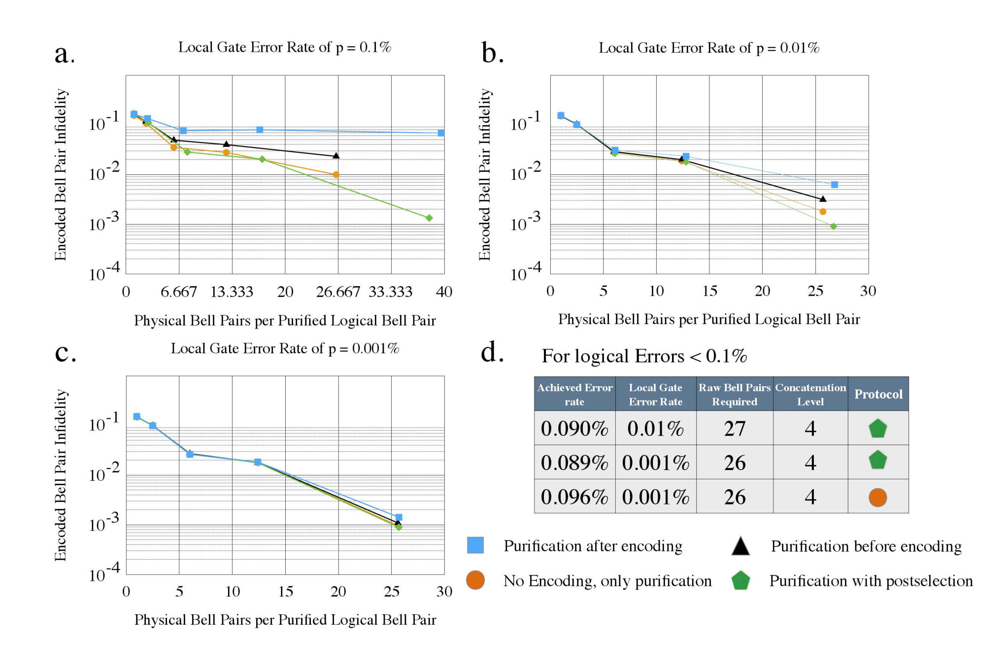
Figure 7.16 shows a similar baseline homogeneous simulation for surface code distance 3.

The difference between purification before encoding and purification of physical Bell pairs indicates how many logical errors are introduced during the encoding process. Purification after encoding may show that the surface code distance 3 is more suitable than the Steane [[7,1,3]], however, because those local gate error rates are greater than the threshold of the Steane [[7,1,3]] code it is hard to judge fairly.
Figure 7.18 plots the number of consumed raw physical Bell pairs versus logical error rate in the output state for the heterogeneous Steane [[7,1,3]]-surface code distance 3 case. This heterogeneous result falls near the average of those two baseline homogeneous simulations above. The is 0.086. The is 1.007. Since the depth of the circuit of the heterogeneous simulation is aligned to the longer depth of the two codes, the heterogeneous result is a bit higher than the average of the homogeneous simulations.
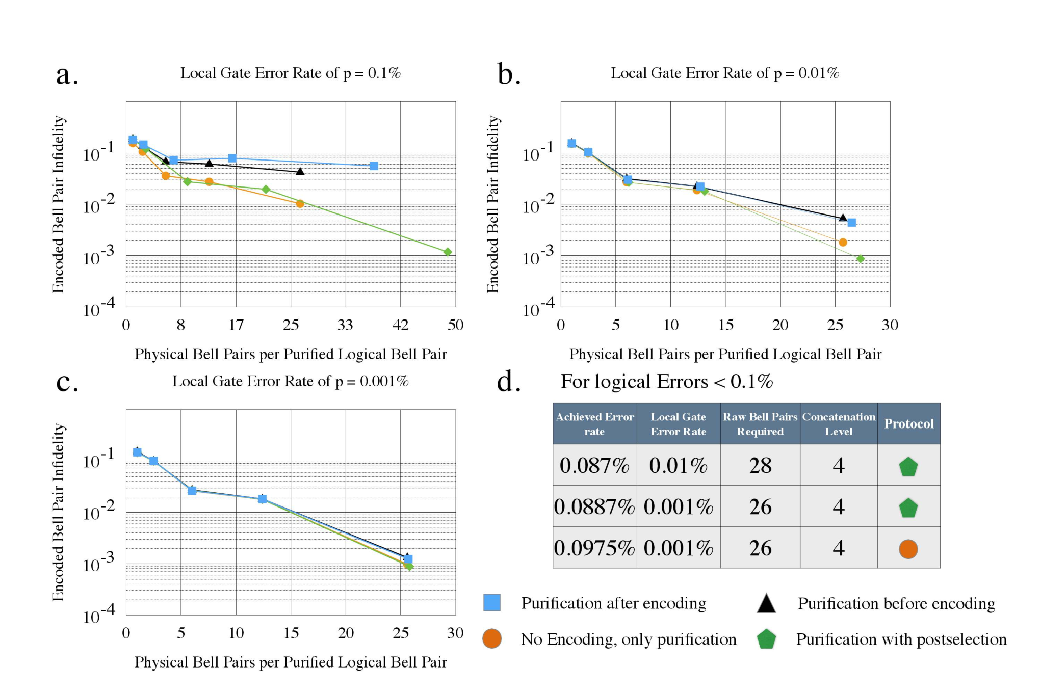
The numbers of raw Bell pairs consumed declines as the local gate error rate is lowered. This is because the influence of the local gate error rate shrinks relative to the infidelity of generated raw Bell pairs. If the system is free from local gate error, the numbers of raw Bell pairs consumed by the three schemes must converge. At , the required number of raw Bell pairs of the schemes are essentially identical and they require about 26 raw Bell pairs to achieve four rounds of purification. Higher efficiency would require improving the initial fidelity of .
At any error rate and with any number of rounds of purification from 0 to 4, purification before encoding and purification after encoding result in fidelity worse than simple purification of physical Bell pairs. This suggests that errors accumulated during encoding are difficult to correct. On the other hand, purification after encoding with strict post-selection gives better results than simple purification, at the expense of consuming more raw physical Bell pairs. This difference is noticeable at ; 49 raw physical Bell pairs are used to create an encoded Bell pair purified four rounds. The local gate error rate is so high that an eigenvalue of -1 is often found at the measurement in purification and the output Bell pair is discarded. For purification after encoding with post-selection, the residual error rate after rounds of purification is similar at any , but resource demands change. It converts local errors into “loss”, or discarded states. Therefore purification after encoding with post-selection is dominated by the original raw Bell pair infidelity. At , purification after encoding also requires more raw physical Bell pairs than the other schemes, because the error rate after purification is so high that the success probability of purification is poor.
Though more rounds of purification are supposed to result in smaller logical error rate, three rounds of purification of purification after encoding at give an error rate larger than that of two rounds. The local gate error rate is too high and purification introduces more errors than it suppresses on odd-numbered purification rounds.
Purification after encoding with strict post-selection gives similar results for the two local gate error rates and . The difference is a small number of consumed raw physical Bell pairs. Even at , we see that four rounds of purification drives the residual error rate down almost to 0.1%. From this fact we conclude that will be a good enough local gate error rate to allow us to create heterogeneously encoded Bell pairs, suitable for many purposes, from raw physical Bell pairs of F=0.85.
Chapter 8 Conclusion
In this Chapter, the conclusion of this dissertation is stated. First the overview of the discussion is summarized. Next the problems, the proposed architecture, and the difficulties to solve the problems are stated. Finally the future work, extendability and importance of this work is summarized.
In this dissertation, a practically scalable distributed quantum computer architecture is proposed in which quantum imperfections including state errors, dynamic losses and static losses are tolerated by quantum error correction, space-efficient error correcting code is employed in memories, and fault-tolerant internal and external data transfer is designed to connect components. Numerical analysis of overhead to tolerate imperfections is completed by analyzing overhead of static losses in this work. It is shown that static losses are tolerable. However, the required resource increase emphasizes the importance of division of computation chip like classical multi-CPU computer and quantum distributed computation. To alleviate the obvious problem of expensive resource requirement, space-saving error correcting code is developed, which should be employed in quantum memories. To connect components such as memories, computation area and network interface, the overhead of fault-tolerant communication of components is numerically analyzed. The importance of parallelism and scalability of internal communication are shown.
To realize a quantum computer, tolerance against imperfections and its overhead is the first thing we have to consider. Fabrication technology for quantum computation is rapidly developing, however, there still large possibility to have problematic devices on the computation chip and it may be difficult to completely get rid of them in the future. Analysis based on ideal assumptions was done, in which concrete methods to deal with static losses are not given.
To realize a quantum computer which is large enough to execute quantum algorithm to solve meaningful problems, resource efficiency is important. Quantum error correcting code requires much computational resource. A logical qubit of the typical surface code, the planar code, consists of physical qubits where is the code distance. Factoring bits requires logical qubits, excluding ancilla qubits for gates and resources for communication. Integration of quantum devices depends on the physical system employed and is limited yet. It is actually infeasible to implement everything on a computation chip, maybe in a machine. Quantum error correcting code which has high error threshold and has small resource requirement has not been found yet.
To realize a quantum computer which has multiple quantum components, fault-tolerant internal networking between any components supporting code conversion is required. Employing multiple error correcting codes had been proposed Scalable internal routing by optical crossbar had been proposed. Concrete means to bridge components which employ heterogeneous error correcting codes and analysis of its overhead are required.
We propose a scalable distributed quantum computer architecture, which tolerates quantum imperfections, has several areas for several purposes in which each area consists of an array of same components of the feasible size to adapt to the overheads caused by tolerating imperfections, and has a core routing module of an optical crossbar which routes photons from components to create entanglement between arbitrary pair of components where imperfections are managed by purification with post-selection after encoding entangled qubits to arbitrary codes. The purposes are computation, memory, ancilla state generation for complex gates and computer networking.
8.1 Difficulties in solving problems
In the analysis of an adaptation of the surface code for static losses, which are manifested as faulty devices on quantum computation chips occurring during fabrication. With this fundamental analysis of static loss and its influence, independent analysis has now been conducted for the three major imperfections of quantum computation for the surface code: state error, dynamic loss, and static loss. The ultimate goal of investigating faulty devices is to support collection of a large pool of sufficiently fault-tolerant quantum computation chips which will be the arrays of components in the computation/memory areas of distributed quantum computers. The method we employ to work around static losses is the code deformation; merging stabilizer units by removing the lost qubits. The surface code on the perfect lattice has complete regularity, but in our case, there come many size of stabilizers in which the order of error syndrome collection is not unified and whose duration differ. To achieve a practical method, we need new two algorithms which is adapted to the quantum error occurrence nature. We determined the order of error syndrome collection by solving traveling salesman problem. There would be a difficulty that solving for big stabilizers may not finish in realistic time, however, later by simulation it is shown that the size of the biggest stabilizer has the strongest correlation with the logical error rate of the defective lattice so that lattices holding such big stabilizers should be discarded anyway; hence this difficulty can be ignored. Another difficulty is how to schedule stabilizers of heterogeneous duration. We solved this difficulty by focusing on the fact that stabilizers of lower frequency may accumulate more physical errors and are easy to lengthen error chains. Therefore we give priority to larger stabilizers hence schedule larger stabilizers first and then schedule small stabilizers repeatedly when member qubits are free.
To develop the space-saving surface code, we have shown an extension of the deformation-based surface code which is capable of close placement by measuring superstabilizers which produce deformation-based qubits. The universality of gates largely influences the flexibility of an error correcting code, which is required for quantum CPU and is useful for quantum memory to realize read and store operations. The space-saving characteristics is the most important factor of this new code, we have to have both characteristics in the same time. We solve this difficulty by a lattice surgery-like CNOT gate for the deformation-based qubits which requires fewer physical qubits than the braiding CNOT gate. Meanwhile we achieve direct conversion from the defect-based surface code to the deformation-based surface code, which can be used as state injection for the deformation-based surface code, then we achieve arbitrary single qubit gate by combining CNOT gate and the arbitrary state injection, hence a universal gate set is completed. The acceptability of close placement and the space-saving CNOT gate allow deformation-based qubits to be packed more tightly than planar code qubits and defect-based qubits.
We have proposed and analyzed a generalized method for creating heterogeneously encoded Bell pairs that can be used for interoperability between encoded quantum components. This is the first step in examining the full design of interconnection of quantum computers/routers/repeaters utilizing different error mitigation techniques. Acquired encoded Bell pairs must have reasonably high fidelity. The fidelity of raw physical Bell pairs are determined by the implementation of components, optical fibers and BSA hence it is physically limited. Hence the method how to increase the fidelity is important and to find the means in which the achievement and resource consumption meets is the difficult thing. To solve this problem, we considered three ways of entanglement purification, purification before encoding, purification after encoding and purification after encoding with strict post-selection and we investigated the relationship of the achieved fidelity and the resource consumption of those three by numerical simulation .
8.2 Quantitative results and overheads
We analyzed our approach against faulty losses by simulation to investigate the relationship between the logical error rates and lattice characteristics of simulated defective lattices. Our approach is to merge stabilizers broken by faulty data qubits to a superstabilizer and to work around faulty ancilla qubits using SWAP gates, without changing the original role of the qubits. Our simulation with single faulty device revealed that faulty qubits at the periphery reduce the logical error rate less than those in the center. Even a single fault has a large impact on the residual error rate. Our simulation with randomly placed faulty devices showed that at yield, the impact on net error rate is significant but many of the chips still achieve break-even by , and therefore could be used in a real-world setting. At yield, very few chips achieve break-even. At yield, almost no chips are usable. Those facts establish the goals for experimental research to build the surface code quantum computer. The simulation of randomly placed faulty devices also showed that discarding bad lattices makes the ensemble better, showing the trade-off between the cost by discarding and the strength of fault-tolerance of an ensemble. Discarding makes the effective code distance of the defective lattice ensemble result in two more longer effective code distance at distance 9 and 13 at yield. yield shows error suppression at obviously practical physical error rates, at around , and discarding works for yield. With a low physical error rate, yield may be sufficient to build a quantum computer. At yield, only very weak error suppression is observed even at . Even 90%-discarding does not show enough error suppression and distance 17 has the highest error rate. We conclude that yield is not suitable for building quantum computer, using the surface code without addtional architectural support. The randomly faulty lattice simulation also revealed that the average of the and the average of the of stabilizers show the strongest correlations to simulated residual error rate among a set of proposed metrics for chip evaluation. The and is the product of the “cycle” which is the average steps the stabilizer is measured by and the number of data qubits/the number of qubits involved in the stabilizer, respectively. Therefore the accumulated error possibilities in a stabilizer may be the most correlated factor to the logical error rate.
We have shown theoretical basic concepts of the deformation-based surface code but have not calculated the error suppression ability since that of the surface code has been investigated well. The superstabilizers which compose deformation-based qubits require steps for stabilizer measurements where is the effective code distance. Our placement design preserves logical qubits as any logical operator passes through a chain of normal stabilizers that compose the effective code distance, . Hence, by adding to the original code distance, the long stabilizer measurement does not degrade the error suppression efficiency. The deformation-based surface code should have residual error rate similar to the conventional surface code of code distance three shorter, and hence conventional error analysis for the surface code can be applied to the deformation-based surface code. Our design requires physical qubits for a logical qubit, compared to the physical qubits required in the conventional design. Our design would halve the resource required to build a large scale quantum computer.
Our purification simulations have shown that purification after encoding with strict post-selection is a better preparation method than our other two candidates. Strict post-selection of two rounds of purification results in better fidelity than error correction of four rounds of purification at all error rates, and better physical Bell pair efficiency. Since the threshold of the error rate of the Steane [[7,1,3]] code is around , our simulations of purification before encoding and purification after encoding of do not show an advantage compared to simple physical purification; however, strict post-selection does. Purification after encoding with strict post-selection has a higher threshold than the normal encoding and purification do. With initial , we can almost reach a residual error rate of using 4 rounds of purification, for physical Bell pairs at or post-selected heterogeneous pairs at . QEC generally corrects up to errors per block, and detects but mis-corrects errors. Post-selection eliminates this mis-correction possibility, leaving only groups of errors or errors that occur after syndrome extraction in the state. The structure of CSS codes is so self-similar that we expect that the analysis will be useful for evaluating other hardware models and CSS codes.
8.3 Future work
We have shown solutions to three problems and analyzed the overhead of them separately. Hence the biggest future work should be the all-in-one analysis of the proposed architecture.
8.3.1 Better way to tolerant against static losses
Faulty data qubits result in merging plaquettes and deepen the stabilizer circuit hence lengthen the “cycle”. Faulty ancilla qubits result in requiring more SWAP gates to walk through data qubits and ancilla qubits surrounding the faulty ancilla qubits. However, our data also shows that the number of faulty ancilla qubits has weak correlation to the residual error rate. Therefore, utilizing an ancilla qubit to substitute for neighboring faulty data qubit and keeping stabilizer sizes at four qubits (three qubits at boundaries) may be an effective solution against static losses.
There is a range in the degree of problems a quantum device has. Some of problematic devices do not work at all. Some of them work but their error rate is higher than regular ones. Some of them execute most gates properly but have problem for some gate. The definition of the problems for a quantum device depends on its purpose. If the definition is fulfilled, it should be a problem. To consider such difference would help designing high performance quantum computer.
8.3.2 More denser placement of the deformation-based code
We have shown the placement in which four logical qubits are grouped to be a unit for the global placement. This design is to enable lattice surgery both on the smooth boundaries and on the rough boundaries. By restricting this flexibility, more space-saving placement may be found.
8.3.3 Combination of purification methods
We employed and simulated purification before encoding, purification after encoding and purification after encoding with strict post-selection separately. Purification before encoding actually works as increase the fidelity of source Bell pairs for encoding, hence there is a possibility that the combination of Purification before encoding and purification after encoding with strict post-selection would result in better balance between the achievement and the resource consumption.
8.4 Diversion of the architecture
Meanwhile, the crossbar switch can be the core module of a quantum router architecture as shown in Figure 8.2 [121].
This router architecture is derived from the architecture of conventional classical router and it has several network interface cards connected to the crossbar switch. Combining the quantum computer architecture and the router architecture and exchanging the logical qubit units with quantum computation chips of the surface code and of other complemental codes, a quantum computer architecture which supports networking and utilizes the benefit of the multiple code model is achieved.
The analysis presented here is useful not only in the abstract, but also serves as a first step toward a hardware design for a multi-protocol quantum router (the boxes in Figure 8.2). Such a router may be built on a quantum multicomputer architecture, with several small quantum computers coupled internally via a local optical network [172, 84, 92, 128]. This allows hardware architects to build separate, small devices to connect to each type of network, then to create Bell pairs between these devices using the method described in this paper. In addition, this method can be used within large-scale quantum computers that wish to use different quantum error correcting codes for different purposes, such as long-term memory or ancilla state preparation.
This scheme is internal to a single repeater at the border of two networks, and will allow effective end-to-end communication where errors across links are more important than errors within a repeater node. It therefore can serve as a building block for a quantum Internet.
8.5 The importance of this work
The feasibility of the quantum computer strongly depends on the error management scheme and on how to get the required computation power from small components available with technologies at that time. This work shows how to get the computation power by connecting such components with limited power, with tolerating quantum imperfections. My architecture and the way to design will be referred from any future work to design quantum computer architectures dedicated to specific fundamental physical technologies.
References
- [1] Muhammad Ahsan, Rodney Van Meter, and Jungsang Kim. Designing a million-qubit quantum computer using a resource performance simulator. ACM Journal on Emerging Technologies in Computing Systems (JETC), 12(4):39, 2015.
- [2] P Aliferis, F Brito, D P DiVincenzo, J Preskill, M Steffen, and B M Terhal. Fault-tolerant computing with biased-noise superconducting qubits: a case study. New Journal of Physics, 11(1):013061, 2009.
- [3] Panos Aliferis and Barbara M. Terhal. Fault-tolerant quantum computation for local leakage faults. Quantum Info. Comput., 7(1):139–156, January 2007.
- [4] Jonas T. Anderson, Guillaume Duclos-Cianci, and David Poulin. Fault-tolerant conversion between the steane and reed-muller quantum codes. Phys. Rev. Lett., 113:080501, Aug 2014.
- [5] Luciano Aparicio and Rodney Van Meter. Multiplexing schemes for quantum repeater networks. volume 8163, pages 816308–816308–12, 2011.
- [6] Luciano Aparicio, Rodney Van Meter, and Hiroshi Esaki. Protocol design for quantum repeater networks. In Proceedings of the 7th Asian Internet Engineering Conference, AINTEC ’11, pages 73–80, New York, NY, USA, 2011. ACM.
- [7] Koji Azuma, Kiyoshi Tamaki, and Hoi-Kwong Lo. All-photonic quantum repeaters. Nat Comms, 6:6787, Apr 2015.
- [8] Dave Bacon. Operator quantum error-correcting subsystems for self-correcting quantum memories. Phys. Rev. A, 73:012340, Jan 2006.
- [9] Sean D. Barrett and Thomas M. Stace. Fault tolerant quantum computation with very high threshold for loss errors. Phys. Rev. Lett., 105(20):200502, Nov 2010.
- [10] Stephen D. Bartlett, Terry Rudolph, and Robert W. Spekkens. Reference frames, superselection rules, and quantum information. Rev. Mod. Phys., 79:555–609, Apr 2007.
- [11] David Beckman, Amalavoyal N. Chari, Srikrishna Devabhaktuni, and John Preskill. Efficient networks for quantum factoring. Phys. Rev. A, 54:1034–1063, Aug 1996.
- [12] Michael Ben-Or and Avinatan Hassidim. Fast quantum byzantine agreement. In Proceedings of the Thirty-seventh Annual ACM Symposium on Theory of Computing, STOC ’05, pages 481–485, New York, NY, USA, 2005. ACM.
- [13] Charles H. Bennett, Gilles Brassard, Claude Crépeau, Richard Jozsa, Asher Peres, and William K. Wootters. Teleporting an unknown quantum state via dual classical and einstein-podolsky-rosen channels. Phys. Rev. Lett., 70:1895–1899, Mar 1993.
- [14] H Bombin and M A Martin-Delgado. Quantum measurements and gates by code deformation. Journal of Physics A: Mathematical and Theoretical, 42(9):095302, 2009.
- [15] Hector Bombin. Gauge color codes: optimal transversal gates and gauge fixing in topological stabilizer codes. New Journal of Physics, 17(8):083002, 2015.
- [16] Dan Boneh and Richard J. Lipton. Quantum Cryptanalysis of Hidden Linear Functions, pages 424–437. Springer Berlin Heidelberg, Berlin, Heidelberg, 1995.
- [17] Michel Boyer, Gilles Brassard, Peter Høyer, and Alain Tapp. Tight bounds on quantum searching. Fortschritte der Physik, 46(4-5):493–505, 1998.
- [18] S. Bravyi and A. Kitaev. Quantum codes on a lattice with boundary. Arxiv preprint quant-ph/9811052, 1998.
- [19] S. Bravyi and A. Kitaev. Universal quantum computation with ideal Clifford gates and noisy ancillas. Physical Review A, 71(2):22316, 2005.
- [20] Sergey Bravyi, Guillaume Duclos-Cianci, David Poulin, and Martin Suchara. Subsystem surface codes with three-qubit check operators. Quantum Info. Comput., 13(11-12):963–985, November 2013.
- [21] Sergey Bravyi and Jeongwan Haah. Magic-state distillation with low overhead. Phys. Rev. A, 86:052329, Nov 2012.
- [22] H.-J. Briegel, W. Dür, J.I. Cirac, and P. Zoller. Quantum repeaters: the role of imperfect local operations in quantum communication. Physical Review Letters, 81:5932–5935, 1998.
- [23] Anne Broadbent, Joseph Fitzsimons, and Elham Kashefi. Measurement-based and universal blind quantum computation. In Alessandro Aldini, Marco Bernardo, Alessandra Di Pierro, and Herbert Wiklicky, editors, Formal Methods for Quantitative Aspects of Programming Languages: 10th International School on Formal Methods for the Design of Computer, Communication and Software Systems, SFM 2010, Bertinoro, Italy, June 21-26, 2010, Advanced Lectures, pages 43–86. Springer Berlin Heidelberg, Berlin, Heidelberg, 2010.
- [24] Katherine L. Brown, William J. Munro, and Vivien M. Kendon. Using quantum computers for quantum simulation. Entropy, 12(11):2268, 2010.
- [25] Todd A. Brun, Yi-Cong Zheng, Kung-Chuan Hsu, Joshua Job, and Ching-Yi Lai. Teleportation-based fault-tolerant quantum computation in multi-qubit large block codes, 2015.
- [26] SidneyD. Buchbinder, ChanningL. Huang, and YaakovS. Weinstein. Encoding an arbitrary state in a [7,1,3] quantum error correction code. Quantum Information Processing, 12(2):699–719, 2013.
- [27] Harry Buhrman, Richard Cleve, Serge Massar, and Ronald de Wolf. Nonlocality and communication complexity. Rev. Mod. Phys., 82:665–698, Mar 2010.
- [28] Harry Buhrman, Richard Cleve, and Avi Wigderson. Quantum vs. classical communication and computation. In Proceedings of the thirtieth annual ACM symposium on Theory of computing, pages 63–68. ACM, 1998.
- [29] Harry Buhrman and Hein Röhrig. Mathematical Foundations of Computer Science 2003, chapter Distributed Quantum Computing, pages 1–20. Springer-Verlag, 2003.
- [30] G S Buller and R J Collins. Single-photon generation and detection. Measurement Science and Technology, 21(1):012002, 2010.
- [31] Iulia Buluta, Sahel Ashhab, and Franco Nori. Natural and artificial atoms for quantum computation. Reports on Progress in Physics, 74(10):104401, 2011.
- [32] Iulia Buluta and Franco Nori. Quantum simulators. Science, 326(5949):108–111, 2009.
- [33] J. Chiaverini, J. Britton, D. Leibfried, E. Knill, M. D. Barrett, R. B. Blakestad, W. M. Itano, J. D. Jost, C. Langer, R. Ozeri, T. Schaetz, and D. J. Wineland. Implementation of the semiclassical quantum Fourier transform in a scalable system. Science, 308:997–1000, 2005.
- [34] Chia-Hung Chien, Rodney Van Meter, and Sy-Yen Kuo. Fault-tolerant operations for universal blind quantum computation. J. Emerg. Technol. Comput. Syst., 12(1):9:1–9:26, August 2015.
- [35] Byung-Soo Choi. Cost comparison between code teleportation and stabilizer sequence methods for quantum code conversion. In ICT Convergence (ICTC), 2013 International Conference on, pages 1083–1087, Oct 2013.
- [36] Byung-Soo Choi. Dual-code quantum computation model. Quantum Information Processing, 14(8):2775–2818, 2015.
- [37] I.L. Chuang. Quantum algorithm for distributed clock synchronization. Physical Review Letters, 85(9):2006–2009, 2000.
- [38] J.I. Cirac, P. Zoller, et al. A scalable quantum computer with ions in an array of microtraps. Nature, 404(6778):579–581, 2000.
- [39] Dean Copsey, Mark Oskin, Frederic T. Chong, Isaac Chuang, and Khaled Abdel-Gaffar. Memory hierarchies for quantum data. In 1st Workshop on Non-Silicon Computing, 2002.
- [40] IBM Corporation. IBM Triples Performance of World’s Fastest, Most Energy-Efficient Supercomputer. http://www-03.ibm.com/press/us/en/pressrelease/21791.wss.
- [41] Claude Creṕeau, Daniel Gottesman, and Adam Smith. Secure multi-party quantum computation. In STOC 2002, pages 643–652. ACM Press, New York, 2002.
- [42] Christopher M. Dawson, Henry L. Haselgrove, and Michael A. Nielsen. Noise thresholds for optical quantum computers. Phys. Rev. Lett., 96:020501, Jan 2006.
- [43] Christopher M. Dawson and Michael A. Nielsen. The Solovay-Kitaev theorem. Quantum Information and Computation, 6(1):81–95, 2006.
- [44] Eric Dennis, Alexei Kitaev, Andrew Landahl, and John Preskill. Topological quantum memory. Journal of Mathematical Physics, 43(9):4452–4505, 2002.
- [45] Simon J Devitt, Austin G Fowler, Ashley M Stephens, Andrew D Greentree, Lloyd C L Hollenberg, William J Munro, and Kae Nemoto. Architectural design for a topological cluster state quantum computer. New Journal of Physics, 11(8):083032, 2009.
- [46] Simon J. Devitt, Andrew D. Greentree, Ashley M. Stephens, and Rodney Van Meter. High-speed quantum networking by ship. Arxiv preprint quant-ph/arXiv:1410.3224, 2014.
- [47] Simon J Devitt, William J Munro, and Kae Nemoto. Quantum error correction for beginners. Reports on Progress in Physics, 76(7):076001, 2013.
- [48] E. W. Dijkstra. A note on two problems in connexion with graphs. Numerische Mathematik, 1(1):269–271, 1959.
- [49] David P DiVincenzo. Fault-tolerant architectures for superconducting qubits. Physica Scripta, 2009(T137):014020, 2009.
- [50] David P. DiVincenzo and IBM. The physical implementation of quantum computation. arXiv:quant-ph/0002077, 2000.
- [51] L.-M. Duan, M. D. Lukin, J. I. Cirac, and P. Zoller. Long-distance quantum communication with atomic ensembles and linear optics. Nature, 414(6862):413–418, 11 2001.
- [52] W. Dür and H.-J. Briegel. Entanglement purification for quantum computation. Physical Review Letters, 90(6):067901, 2003.
- [53] W. Dür, H.-J. Briegel, J. I. Cirac, and P. Zoller. Quantum repeaters based on entanglement purification. Physical Review A, 59(1):169–181, Jan 1999.
- [54] W. Dür and H.J. Briegel. Entanglement purification and quantum error correction. Rep. Prog. Phys., 70:1381–1424, 2007.
- [55] C. Dürr, M. Heiligman, P. Høyer, and M. Mhalla. Quantum query complexity of some graph problems. In Proceedings of 31st International Conference on Automata, Languages and Programming (ICALP’04), page 481–493, 2004.
- [56] Christoph Dürr and Peter Høyer. A quantum algorithm for finding the minimum. arXiv:quant-ph/9607014, 1996.
- [57] Chip Elliott, Alexander Colvin, David Pearson, Oleksiy Pikalo, John Schlafer, and Henry Yeh. Current status of the DARPA quantum network (invited paper). volume 5815, pages 138–149, Proc. SPIE 5815, 2005.
- [58] Richard P Feynman. Simulating physics with computers. International journal of theoretical physics, 21(6):467–488, 1982.
- [59] A. Fowler, A. Whiteside, A. McInnes, and A. Rabbani. Topological code Autotune. Physical Review X, 2(4), Oct 2012.
- [60] A. G. Fowler, S. J. Devitt, and L. C. L. Hollenberg. Implementation of shor’s algorithm on a linear nearest neighbour qubit array. Quantum Info. Comput., 4(4):237–251, July 2004.
- [61] Austin G. Fowler and Simon J. Devitt. A bridge to lower overhead quantum computation. arXiv:1209.0510, 2012.
- [62] Austin G. Fowler, Matteo Mariantoni, John M. Martinis, and Andrew N. Cleland. Surface codes: Towards practical large-scale quantum computation. Phys. Rev. A, 86:032324, Sep 2012.
- [63] Austin G. Fowler, Ashley M. Stephens, and Peter Groszkowski. High-threshold universal quantum computation on the surface code. Phys. Rev. A, 80(5):052312, Nov 2009.
- [64] Austin G. Fowler, William F. Thompson, Zhizhong Yan, Ashley M. Stephens, B. L. T. Plourde, and Frank K. Wilhelm. Long-range coupling and scalable architecture for superconducting flux qubits. Phys. Rev. B, 76:174507, Nov 2007.
- [65] Austin G. Fowler, David S. Wang, Charles D. Hill, Thaddeus D. Ladd, Rodney Van Meter, and Lloyd C. L. Hollenberg. Surface code quantum communication. Phys. Rev. Lett., 104(18):180503, May 2010.
- [66] I. M. Georgescu, S. Ashhab, and Franco Nori. Quantum simulation. Rev. Mod. Phys., 86:153–185, Mar 2014.
- [67] Daniel Gottesman. Stabilizer Codes and Quantum Error Correction. PhD thesis, California Institute of Technology, 1997.
- [68] Lov K. Grover. Quantum mechanics helps in searching for a needle in a haystack. Phys. Rev. Lett., 79:325–328, Jul 1997.
- [69] Henry L. Haselgrove and Peter P. Rohde. Trade-off between the tolerance of located and unlocated errors in nondegenerate quantum error-correcting codes. Quantum Information and Computation, 8:0399–0410, 2008.
- [70] A. J. F. Hayes, H. L. Haselgrove, Alexei Gilchrist, and T. C. Ralph. Fault tolerance in parity-state linear optical quantum computing. Phys. Rev. A, 82:022323, Aug 2010.
- [71] John L. Hennessy and David A. Patterson. Computer Architecture, Fifth Edition: A Quantitative Approach. Morgan Kaufmann Publishers Inc., San Francisco, CA, USA, 5th edition, 2011.
- [72] Thomas Herbst, Thomas Scheidl, Matthias Fink, Johannes Handsteiner, Bernhard Wittmann, Rupert Ursin, and Anton Zeilinger. Teleportation of entanglement over 143 km. Proceedings of the Natural Academy of Sciences of the United Statesof America, 112(46):14202–14205, 2015.
- [73] Charles D. Hill, Austin G. Fowler, David S. Wang, and Lloyd C. L. Hollenberg. Fault-tolerant quantum error correction code conversion. Quantum Info. Comput., 13(5-6):439–451, May 2013.
- [74] Charles D. Hill, Eldad Peretz, Samuel J. Hile, Matthew G. House, Martin Fuechsle, Sven Rogge, Michelle Y. Simmons, and Lloyd C. L. Hollenberg. A surface code quantum computer in silicon. Science Advances, 1(9), 2015.
- [75] R. Hisatomi, A. Osada, Y. Tabuchi, T. Ishikawa, A. Noguchi, R. Yamazaki, K. Usami, and Y. Nakamura. Bidirectional conversion between microwave and light via ferromagnetic magnons. Phys. Rev. B, 93:174427, May 2016.
- [76] L. C. L. Hollenberg, A. D. Greentree, A. G. Fowler, and C. J. Wellard. Two-dimensional architectures for donor-based quantum computing. Phys. Rev. B, 74:045311, Jul 2006.
- [77] C. K. Hong, Z. Y. Ou, and L. Mandel. Measurement of subpicosecond time intervals between two photons by interference. Phys. Rev. Lett., 59:2044–2046, Nov 1987.
- [78] Clare Horsman, Austin G Fowler, Simon Devitt, and Rodney Van Meter. Surface code quantum computing by lattice surgery. New Journal of Physics, 14:123011, December 2012.
- [79] IEEE. IEEE Standard for Information Technology - Telecommunications and Information Exchange Between Systems - Local and Metropolitan Area Networks - Specific Requirements Part 3: Carrier Sense Multiple Access with Collision Detection (CSMA/CD) Access Method and Physical Layer Specifications. IEEE Std 802.3-2005 (Revision of IEEE Std 802.3-2002 including all approved amendments), pages 1–2695, Dec 2005.
- [80] Rodney Doyle Van Meter III. Architecture of a Quantum Multicomputer Optimized for Shor’s Factoring Algorithm. PhD thesis, Keio University, 2006.
- [81] Takahiro Inagaki, Nobuyuki Matsuda, Osamu Tadanaga, Masaki Asobe, and Hiroki Takesue. Entanglement distribution over 300 km of fiber. Opt. Express, 21(20):23241–23249, Oct 2013.
- [82] Liang Jiang, J. M. Taylor, Kae Nemoto, W. J. Munro, Rodney Van Meter, and M. D. Lukin. Quantum repeater with encoding. Phys. Rev. A, 79:032325, Mar 2009.
- [83] Liang Jiang, Jacob M. Taylor, Navin Khaneja, and Mikhail D. Lukin. Optimal approach to quantum communication using dynamic programming. Proceedings of the National Academy of Sciences, 104(44):17291–17296, 2007.
- [84] Liang Jiang, Jacob M. Taylor, Anders S. Sørensen, and Mikhail D. Lukin. Distributed quantum computation based on small quantum registers. Phys. Rev. A, 76:062323, Dec 2007.
- [85] Tomas Jochym-O’Connor and Raymond Laflamme. Using concatenated quantum codes for universal fault-tolerant quantum gates. Phys. Rev. Lett., 112:010505, Jan 2014.
- [86] Cody Jones, Mark F. Gyure, Thaddeus D. Ladd, Michael A. Fogarty, Andrea Morello, and Andrew S. Dzurak. A logical qubit in a linear array of semiconductor quantum dots. arXiv:1608.06335, 2016.
- [87] N. Cody Jones, Rodney Van Meter, Austin G. Fowler, Peter L. McMahon, Jungsang Kim, Thaddeus D. Ladd, and Yoshihisa Yamamoto. Layered architecture for quantum computing. Phys. Rev. X, 2:031007, Jul 2012.
- [88] N.C. Jones, J.D. Whitfield, P.L. McMahon, M.H. Yung, R. Van Meter, A. Aspuru-Guzik, and Y. Yamamoto. Faster quantum chemistry simulation on fault-tolerant quantum computers. New Journal of Physics, 14(11):115023, 2012.
- [89] Stephen Jordan. Quantum algorithm zoo. http://math.nist.gov/quantum/zoo/.
- [90] R. Jozsa, D.S. Abrams, J.P. Dowling, and C.P. Williams. Quantum clock synchronization based on shared prior entanglement. Physical Review Letters, 85(9):2010–2013, 2000.
- [91] J. Kim et al. 1100x1100 port MEMS-based optical crossconnect with 4-dB maximum loss. IEEE Photonics Technology Letters, 15(11):1537–1539, 2003.
- [92] Jungsang Kim and Changsoon Kim. Integrated optical approach to trapped ion quantum computation. qic, 9(2), 2009.
- [93] H. J. Kimble. The quantum internet. Nature, 453(7198):1023–1030, Jun 2008.
- [94] A.Y. Kitaev. Fault-tolerant quantum computation by anyons. Annals of Physics, 303(1):2–30, 2003.
- [95] M. Kleinmann, H. Kampermann, T. Meyer, and D. Bruß. Physical purification of quantum states. Phys. Rev. A, 73:062309, Jun 2006.
- [96] E. Knill. Scalable quantum computing in the presence of large detected-error rates. Phys. Rev. A, 71:042322, Apr 2005.
- [97] E. Knill and R. Laflamme. Concatenated quantum codes. http://arXiv.org/quant-ph/9608012, August 1996.
- [98] Pieter Kok, W. J. Munro, Kae Nemoto, T. C. Ralph, Jonathan P. Dowling, and G. J. Milburn. Linear optical quantum computing with photonic qubits. Rev. Mod. Phys., 79:135–174, Jan 2007.
- [99] Vladimir Kolmogorov. Blossom V: a new implementation of a minimum cost perfect matching algorithm. Mathematical Programming Computation, 1:43–67, 2009.
- [100] P. Kómár, E.M. Kessler, M. Bishof, L. Jiang, A. S. Sorensen, and M. D. Lukin. A quantum network of clocks. Nature Physics, June 2014.
- [101] B. Korzh, N. Walenta, T. Lunghi, N. Gisin, and H. Zbinden. Free-running ingaas single photon detector with 1 dark count per second at 10% efficiency. Applied Physics Letters, 104(8), 2014.
- [102] Richard Kueng, David M. Long, Andrew C. Doherty, and Steven T. Flammia. Comparing experiments to the fault-tolerance threshold. arXiv:1510.05653, 2015.
- [103] T.D. Ladd, F. Jelezko, R. Laflamme, Y. Nakamura, C. Monroe, and J.L. O’Brien. Quantum computers. Nature, 464:45–53, march 2010.
- [104] Andrew J. Landahl, Jonas T. Anderson, and Patrick R. Rice. Fault-tolerant quantum computing with color codes. arXiv preprint arXiv:1108.5738, 2011.
- [105] Ying Li, Sean D Barrett, Thomas M Stace, and Simon C Benjamin. Long range failure-tolerant entanglement distribution. New Journal of Physics, 15(2):023012, 2013.
- [106] Daniel A. Lidar and Todd A. Brun, editors. Quantum Error Correction. Cambridge University Press, 2013.
- [107] Netanel H. Lindner and Terry Rudolph. Proposal for pulsed on-demand sources of photonic cluster state strings. Phys. Rev. Lett., 103:113602, Sep 2009.
- [108] Hoi-Kwong Lo, Tim Spiller, and Sandu Popescu, editors. Introduction to Quantum Computation and Information. World Scientific, 1998.
- [109] Sebastian Mehl, Hendrik Bluhm, and David P. DiVincenzo. Fault-tolerant quantum computation for singlet-triplet qubits with leakage errors. Phys. Rev. B, 91:085419, Feb 2015.
- [110] Tzvetan S. Metodi, Arvin I. Faruque, and Frederic T. Chong. Quantum computing for computer architects, second edition. Synthesis Lectures on Computer Architecture, 6(1):1–203, 2011.
- [111] Tzvetan S. Metodi, Darshan D. Thaker, and Andrew W. Cross. A quantum logic array microarchitecture: Scalable quantum data movement and computation. In Proceedings of the 38th Annual IEEE/ACM International Symposium on Microarchitecture, MICRO 38, pages 305–318, Washington, DC, USA, 2005. IEEE Computer Society.
- [112] Toshiyuki Miyachi, Ken-ichi Chinen, and Yoichi Shinoda. StarBED and SpringOS: Large-scale General Purpose Network Testbed and Supporting Software. In Proceedings of the 1st International Conference on Performance Evaluation Methodologies and Tools, valuetools ’06, New York, NY, USA, 2006. ACM.
- [113] Toshiyuki Miyachi, Takeshi Nakagawa, Ken-ichi Chinen, Shinsuke Miwa, and Yoichi Shinoda. StarBED and SpringOS Architectures and Their Performance, pages 43–58. Springer Berlin Heidelberg, Berlin, Heidelberg, 2012.
- [114] C. Monroe, R. Raussendorf, A. Ruthven, K. R. Brown, P. Maunz, L.-M. Duan, and J. Kim. Large-scale modular quantum-computer architecture with atomic memory and photonic interconnects. Phys. Rev. A, 89:022317, Feb 2014.
- [115] Ashley Montanaro. Quantum pattern matching fast on average. Algorithmica, pages 1–24, 2015.
- [116] Ashley Montanaro. Quantum algorithms: an overview. Npj Quantum Information, 2(15023), January 2016.
- [117] Gordon E. Moore. Cramming more components onto integrated circuits. Electronics, 38(8), April 1965.
- [118] W. J. Munro, A. M. Stephens, S. J. Devitt, K. A. Harrison, and Kae Nemoto. Quantum communication without the necessity of quantum memories. Nature Photonics, 6(11):777–781, 11 2012.
- [119] William J Munro, Simon J Devitt, and Kae Nemoto. Designing quantum repeaters and networks. In SPIE Optical Engineering+ Applications, pages 816307–816307. International Society for Optics and Photonics, 2011.
- [120] WJ Munro, KA Harrison, AM Stephens, SJ Devitt, and K. Nemoto. From quantum multiplexing to high-performance quantum networking. Nature Photonics, 4:792–796, 2010.
- [121] Shota Nagayama, Byung-Soo Choi, Simon Devitt, Shigeya Suzuki, and Rodney Van Meter. Interoperability in encoded quantum repeater networks. Phys. Rev. A, 93:042338, Apr 2016.
- [122] Shota Nagayama, Austin G Fowler, Dominic Horsman, Simon J Devitt, and Rodney Van Meter. Surface code error correction on a defective lattice. New Journal of Physics, 19(2):023050, 2017.
- [123] Shota Nagayama, Takahiko Satoh, and Rodney Van Meter. State injection, lattice surgery, and dense packing of the deformation-based surface code. Phys. Rev. A, 95:012321, Jan 2017.
- [124] Chandra M Natarajan, Michael G Tanner, and Robert H Hadfield. Superconducting nanowire single-photon detectors: physics and applications. Superconductor Science and Technology, 25(6):063001, 2012.
- [125] Naomi H. Nickerson, Ying Li, and Simon C. Benjamin. Topological quantum computing with a very noisy network and local error rates approaching one percent. Nature Communications, 4:1756, Apr 2013.
- [126] Michael A. Nielsen and Isaac L. Chuang. Quantum Computation and Quantum Information. Cambridge University Press, 2000.
- [127] Christian Nölleke, Andreas Neuzner, Andreas Reiserer, Carolin Hahn, Gerhard Rempe, and Stephan Ritter. Efficient teleportation between remote single-atom quantum memories. Phys. Rev. Lett., 110:140403, Apr 2013.
- [128] Daniel K. L. Oi, Simon J. Devitt, and Lloyd C. L. Hollenberg. Scalable error correction in distributed ion trap computers. pra, 74:052313, 2006.
- [129] A. Osada, R. Hisatomi, A. Noguchi, Y. Tabuchi, R. Yamazaki, K. Usami, M. Sadgrove, R. Yalla, M. Nomura, and Y. Nakamura. Cavity optomagnonics with spin-orbit coupled photons. Phys. Rev. Lett., 116:223601, Jun 2016.
- [130] M. Oskin, F.T. Chong, and I.L. Chuang. A practical architecture for reliable quantum computers. Computer, 35(1):79–87, Jan 2002.
- [131] Adam Paetznick and Ben W. Reichardt. Universal fault-tolerant quantum computation with only transversal gates and error correction. Phys. Rev. Lett., 111:090505, Aug 2013.
- [132] Alexandru Paler, Simon J. Devitt, Kae Nemoto, and Ilia Polian. Mapping of topological quantum circuits to physical hardware. Scientific Reports, 4(4657), April 2014.
- [133] Archimedes Pavlidis and Dimitris Gizopoulos. Fast Quantum Modular Exponentiation Architecture for Shor’s Factoring Algorithm. Quantum Info. Comput., 14(7&8):649–682, May 2014.
- [134] M Peev, C Pacher, R Alléaume, C Barreiro, J Bouda, W Boxleitner, T Debuisschert, E Diamanti, M Dianati, J F Dynes, S Fasel, S Fossier, M Fürst, J-D Gautier, O Gay, N Gisin, P Grangier, A Happe, Y Hasani, M Hentschel, H Hübel, G Humer, T Länger, M Legré, R Lieger, J Lodewyck, T Lorünser, N Lütkenhaus, A Marhold, T Matyus, O Maurhart, L Monat, S Nauerth, J-B Page, A Poppe, E Querasser, G Ribordy, S Robyr, L Salvail, A W Sharpe, A J Shields, D Stucki, M Suda, C Tamas, T Themel, R T Thew, Y Thoma, A Treiber, P Trinkler, R Tualle-Brouri, F Vannel, N Walenta, H Weier, H Weinfurter, I Wimberger, Z L Yuan, H Zbinden, and A Zeilinger. The SECOQC quantum key distribution network in Vienna. New Journal of Physics, 11(7):075001, 2009.
- [135] Tien Trung Pham, Rodney Van Meter, and Clare Horsman. Optimization of the Solovay-Kitaev algorithm. Phys. Rev. A, 87:052332, May 2013.
- [136] Ilia Polian and Austin G. Fowler. Design automation challenges for scalable quantum architectures. In Proceedings of the 52Nd Annual Design Automation Conference, DAC ’15, pages 61:1–61:6, New York, NY, USA, 2015. ACM.
- [137] David Poulin. Stabilizer Formalism for Operator Quantum Error Correction. Phys. Rev. Lett., 95:230504, Dec 2005.
- [138] John Preskill. Reliable Quantum Computers. Proc. Roy. Soc. Lond. A, 454:385–410, 1998.
- [139] H Ramesh and V Vinay. String matching in o(n+m ) quantum time. Journal of Discrete Algorithms, 1(1):103 – 110, 2003. Combinatorial Algorithms.
- [140] R. Raussendorf, J. Harrington, and K. Goyal. A fault-tolerant one-way quantum computer. Annals of Physics, 321(9):2242 – 2270, 2006.
- [141] Robert Raussendorf and Hans J. Briegel. A one-way quantum computer. Phys. Rev. Lett., 86:5188–5191, May 2001.
- [142] Robert Raussendorf and Jim Harrington. Fault-tolerant quantum computation with high threshold in two dimensions. Phys. Rev. Lett., 98:190504, May 2007.
- [143] Robert Raussendorf, Jim Harrington, and Kovid Goyal. Topological fault-tolerance in cluster state quantum computation. New Journal of Physics, 9:199, 2007.
- [144] Peter P. Rohde, Timothy C. Ralph, and William J. Munro. Error tolerance and tradeoffs in loss- and failure-tolerant quantum computing schemes. Phys. Rev. A, 75:010302, Jan 2007.
- [145] Nicolas Sangouard, Christoph Simon, Hugues de Riedmatten, and Nicolas Gisin. Quantum repeaters based on atomic ensembles and linear optics. Rev. Mod. Phys., 83:33–80, Mar 2011.
- [146] M. Sasaki, M. Fujiwara, H. Ishizuka, W. Klaus, K. Wakui, M. Takeoka, S. Miki, T. Yamashita, Z. Wang, A. Tanaka, K. Yoshino, Y. Nambu, S. Takahashi, A. Tajima, A. Tomita, T. Domeki, T. Hasegawa, Y. Sakai, H. Kobayashi, T. Asai, K. Shimizu, T. Tokura, T. Tsurumaru, M. Matsui, T. Honjo, K. Tamaki, H. Takesue, Y. Tokura, J. F. Dynes, A. R. Dixon, A. W. Sharpe, Z. L. Yuan, A. J. Shields, S. Uchikoga, M. Legré, S. Robyr, P. Trinkler, L. Monat, J.-B. Page, G. Ribordy, A. Poppe, A. Allacher, O. Maurhart, T. Länger, M. Peev, and A. Zeilinger. Field test of quantum key distribution in the tokyo qkd network. Opt. Express, 19(11):10387–10409, May 2011.
- [147] Peter Selinger. Efficient Clifford+T approximation of single-qubit operators. arXiv:1212.6253 [quant-ph], 2012.
- [148] Peter Selinger. Efficient clifford+ t approximation of single-qubit operators. Quantum Information & Computation, 15(1-2):159–180, 2015.
- [149] Peter W. Shor. Algorithms for quantum computation: Discrete logarithms and factoring. In Proc. 35th Symposium on Foundations of Computer Science, pages 124–134, Los Alamitos, CA, 1994. IEEE Computer Society Press.
- [150] Peter W. Shor. Scheme for reducing decoherence in quantum computer memory. Phys. Rev. A, 52:R2493–R2496, Oct 1995.
- [151] Thomas M. Stace and Sean D. Barrett. Error correction and degeneracy in surface codes suffering loss. Phys. Rev. A, 81:022317, Feb 2010.
- [152] Thomas M. Stace, Sean D. Barrett, and Andrew C. Doherty. Thresholds for topological codes in the presence of loss. Phys. Rev. Lett., 102:200501, May 2009.
- [153] Andrew Steane. Multiple-particle interference and quantum error correction. Proceedings of the Royal Society of London A: Mathematical, Physical and Engineering Sciences, 452(1954):2551–2577, 1996.
- [154] Andrew Steane. Quantum Reed-Muller Codes. arXiv:quant-ph/9608026, 1996.
- [155] Andrew M. Steane. Efficient fault-tolerant quantum computing. Nature, 399(6732):124–126, 5 1999.
- [156] Andrew M. Steane. Overhead and noise threshold of fault-tolerant quantum error correction. Phys. Rev. A, 68:042322, Oct 2003.
- [157] Ashley M. Stephens, Zachary W. E. Evans, Simon J. Devitt, and Lloyd C. L. Hollenberg. Asymmetric quantum error correction via code conversion. Phys. Rev. A, 77:062335, Jun 2008.
- [158] Martin Suchara, Arvin Faruque, Ching-Yi Lai, Gerardo Paz, Frederic T. Chong, and John Kubiatowicz. Comparing the overhead of topological and concatenated quantum error correction. arXiv:1312.2316, 2013.
- [159] K.M. Svore, D.P. DiVincenzo, and B.M. Terhal. Noise threshold for a fault-tolerant two-dimensional lattice architecture. Quantum Information & Computation, 7(4):297–318, 2007.
- [160] Yutaka Tabuchi, Seiichiro Ishino, Toyofumi Ishikawa, Rekishu Yamazaki, Koji Usami, and Yasunobu Nakamura. Hybridizing ferromagnetic magnons and microwave photons in the quantum limit. Phys. Rev. Lett., 113:083603, Aug 2014.
- [161] Yutaka Tabuchi, Seiichiro Ishino, Atsushi Noguchi, Toyofumi Ishikawa, Rekishu Yamazaki, Koji Usami, and Yasunobu Nakamura. Coherent coupling between a ferromagnetic magnon and a superconducting qubit. Science, 349(6246):405–408, 2015.
- [162] Yasuhiro Takahashi and Noboru Kunihiro. A quantum circuit for shor’s factoring algorithm using 2n + 2 qubits. Quantum Info. Comput., 6(2):184–192, March 2006.
- [163] Masahiro Takeoka, Saikat Guha, and Mark M Wilde. Fundamental rate-loss tradeoff for optical quantum key distribution. Nature communications, 5, 2014.
- [164] Barbara M. Terhal. Quantum error correction for quantum memories. Rev. Mod. Phys., 87:307–346, Apr 2015.
- [165] Darshan D. Thaker, Tzvetan S. Metodi, Andrew W. Cross, Isaac L. Chuang, and Frederic T. Chong. Quantum memory hierarchies: Efficient designs to match available parallelism in quantum computing. SIGARCH Comput. Archit. News, 34(2):378–390, May 2006.
- [166] Giuseppe Vallone, Davide Bacco, Daniele Dequal, Simone Gaiarin, Vincenza Luceri, Giuseppe Bianco, and Paolo Villoresi. Experimental satellite quantum communications. Phys. Rev. Lett., 115:040502, Jul 2015.
- [167] P. van Loock, T. D. Ladd, K. Sanaka, F. Yamaguchi, Kae Nemoto, W. J. Munro, and Y. Yamamoto. Hybrid quantum repeater using bright coherent light. Phys. Rev. Lett., 96:240501, Jun 2006.
- [168] R. Van Meter. Quantum networking and internetworking. Network, IEEE, 26(4):59–64, July 2012.
- [169] Rodney Van Meter. Quantum Networking. WILEY, 2014.
- [170] Rodney Van Meter and Clare Horsman. A blueprint for building a quantum computer. Commun. ACM, 56(10):84–93, October 2013.
- [171] Rodney Van Meter and Kohei M. Itoh. Fast quantum modular exponentiation. Phys. Rev. A, 71:052320, May 2005.
- [172] Rodney Van Meter, Thaddeus D. Ladd, Austin G. Fowler, and Yoshihisa Yamamoto. Distributed quantum computation architecture using semiconductor nanophotonics. International Journal of Quantum Information, 8:295–323, 2010.
- [173] Rodney Van Meter, W. J. Munro, Kae Nemoto, and Kohei M. Itoh. Arithmetic on a distributed-memory quantum multicomputer. J. Emerg. Technol. Comput. Syst., 3(4):2:1–2:23, January 2008.
- [174] Rodney Van Meter, Kae Nemoto, W. J. Munro, and Kohei M. Itoh. Distributed arithmetic on a quantum multicomputer. SIGARCH Comput. Archit. News, 34(2):354–365, May 2006.
- [175] Michael Varnava, Daniel E. Browne, and Terry Rudolph. Loss tolerance in one-way quantum computation via counterfactual error correction. Phys. Rev. Lett., 97:120501, Sep 2006.
- [176] Vlatko Vedral, Adriano Barenco, and Artur Ekert. Quantum networks for elementary arithmetic operations. Phys. Rev. A, 54:147–153, Jul 1996.
- [177] Walter Vinci and Daniel A. Lidar. Optimally stopped optimization. arXiv:1608.05764, 2016.
- [178] Joel J Wallman, Marie Barnhill, and Joseph Emerson. Robust characterization of leakage errors. New Journal of Physics, 18(4):043021, 2016.
- [179] Adam C. Whiteside and Austin G. Fowler. Practical topological cluster state quantum computing requires loss below 1%. arXiv:1409.4880, 2014.
- [180] Mark G. Whitney, Nemanja Isailovic, Yatish Patel, and John Kubiatowicz. A fault tolerant, area efficient architecture for shor’s factoring algorithm. SIGARCH Comput. Archit. News, 37(3):383–394, June 2009.
- [181] Norman Y. Yao, Liang Jiang, Alexey V. Gorshkov, Peter C. Maurer, Geza Giedke, J. Ignacio Cirac, and Mikhail D. Lukin. Scalable architecture for a room temperature solid-state quantum information processor. Nature Communications, 3(800), December 2012.
- [182] M. Zwerger, W. Dür, and H. J. Briegel. Measurement-based quantum repeaters. Phys. Rev. A, 85:062326, Jun 2012.
Appendix A Supplemental graphs for the defective lattice analysis
This appendix shows supplemental graphs to visualize the effect of culling and raw data of the surface code on the defective lattice.
A.1 Graphs to compare culled pools
Figure A.2 shows the graphs between yields and logical error rates at specific physical error rates.


A.2 Scatterplots of randomly defective lattices
Figures A.4, A.6, A.8, A.10 and A.12 show the scatter plots of raw data of randomly defective lattices. Figure A.6 shows an outlier chip. Actually the lattice on the chip has worse logical error rate as logical error rate. The lattice by chance has faulty devices which deform the left and the right boundaries to be close with preserving the top and the bottom boundaries apart. Because of the largely deformed shape of the lattice, the usable area of the lattice is narrow and there are only few faulty devices on the usable area which increase logical error rates. Hence the chip exhibits stronger tolerance against logical error than others.


Appendix B Supplemental data in encoding Bell pairs heterogeneously
B.1 Simulation data for raw Bell pairs on multi-NIC router architecture
Table B.2 shows our baseline simulation results using physical entanglement only with no encoding. Table B.4 shows the simulated results of purification before encoding for a Bell pair of a single layer of the Steane [[7,1,3]] code and a distance 3 surface code. Table B.6 shows the simulated results of the scheme purification after encoding of the same codes. Table B.8 shows the simulated results of the scheme purification after encoding with strict post-selection. Since purification at the level of encoded qubits consists of logical gates, purification before encoding has a much smaller KQ than the other two schemes. Purification after encoding with strict post-selection discards more qubits than purification after encoding does to create a purified encoded Bell pair, so that purification after encoding with strict post-selection also results in a larger KQ. Table B.10 shows the simulated results of the scheme purification after encoding with strict post-selection between the Steane [[7,1,3]] code and the non-encoded physical half. Table B.12 shows the simulated results of the scheme purification after encoding with strict post-selection between the distance three surface code and the non-encoded physical half.
(a)The local gate error rate is .
| #purifi- | X error | Z error | Merged | Phys. | KQ | #single | #two |
|---|---|---|---|---|---|---|---|
| cation | rate | rate | error | Bell Pair | qubit | qubit | |
| rate | Ineff. | gate | gate | ||||
| 0 | 0.113 | 0.1 | 0.156 | 1.0 | 88 | 86 | 1 |
| 1 | 0.096 | 0.0197 | 0.106 | 2.5 | 98 | 91 | 5 |
| 2 | 0.0247 | 0.0154 | 0.036 | 6.0 | 122 | 103 | 14 |
| 3 | 0.0248 | 0.00498 | 0.0275 | 12.6 | 167 | 125 | 32 |
| 4 | 0.00753 | 0.00523 | 0.0103 | 26.4 | 262 | 173 | 70 |
(b)The local gate error rate is .
| #purifi- | X error | Z error | Merged | Phys. | KQ | #single | #two |
|---|---|---|---|---|---|---|---|
| cation | rate | rate | error | Bell Pair | qubit | qubit | |
| rate | Ineff. | gate | gate | ||||
| 0 | 0.109 | 0.0968 | 0.151 | 1.0 | 88 | 86 | 1 |
| 1 | 0.0915 | 0.0151 | 0.0988 | 2.5 | 98 | 91 | 5 |
| 2 | 0.0183 | 0.0104 | 0.0271 | 6.0 | 122 | 103 | 14 |
| 3 | 0.0183 | 0.000796 | 0.0189 | 12.4 | 166 | 125 | 32 |
| 4 | 0.00125 | 0.000796 | 0.00182 | 25.7 | 258 | 171 | 68 |
(c)The local gate error rate is .
| #purifi- | X error | Z error | Merged | Phys. | KQ | #single | #two |
|---|---|---|---|---|---|---|---|
| cation | rate | rate | error | Bell Pair | qubit | qubit | |
| rate | Ineff. | gate | gate | ||||
| 0 | 0.112 | 0.0963 | 0.152 | 1.0 | 88 | 86 | 1 |
| 1 | 0.0928 | 0.0152 | 0.101 | 2.5 | 98 | 91 | 5 |
| 2 | 0.0177 | 0.0102 | 0.0262 | 6.0 | 121 | 103 | 14 |
| 3 | 0.0176 | 0.000381 | 0.0179 | 12.4 | 166 | 125 | 32 |
| 4 | 0.000633 | 0.000371 | 0.000975 | 25.6 | 257 | 171 | 68 |
(a)The local gate error rate is .
| #purifi- | X error | Z error | Merged | Phys. | KQ | #single | #two |
|---|---|---|---|---|---|---|---|
| cation | rate | rate | error | Bell Pair | qubit | qubit | |
| rate | Ineff. | gate | gate | ||||
| 0 | 0.128 | 0.12 | 0.188 | 1.0 | 5402 | 4130 | 636 |
| 1 | 0.111 | 0.0379 | 0.135 | 2.5 | 5412 | 4135 | 640 |
| 2 | 0.0402 | 0.0355 | 0.0674 | 6.0 | 5436 | 4147 | 649 |
| 3 | 0.0421 | 0.0258 | 0.061 | 12.6 | 5481 | 4170 | 667 |
| 4 | 0.0231 | 0.0251 | 0.0424 | 26.4 | 5576 | 4217 | 705 |
(b)The local gate error rate is .
| #purifi- | X error | Z error | Merged | Phys. | KQ | #single | #two |
|---|---|---|---|---|---|---|---|
| cation | rate | rate | error | Bell Pair | qubit | qubit | |
| rate | Ineff. | gate | gate | ||||
| 0 | 0.114 | 0.0976 | 0.155 | 1.0 | 5402 | 4130 | 636 |
| 1 | 0.0927 | 0.0173 | 0.102 | 2.5 | 5412 | 4135 | 640 |
| 2 | 0.02 | 0.0136 | 0.0315 | 6.0 | 5436 | 4147 | 649 |
| 3 | 0.0201 | 0.00293 | 0.0224 | 12.4 | 5480 | 4169 | 667 |
| 4 | 0.00298 | 0.0029 | 0.00529 | 25.7 | 5572 | 4215 | 703 |
(c)The local gate error rate is .
| #purifi- | X error | Z error | Merged | Phys. | KQ | #single | #two |
|---|---|---|---|---|---|---|---|
| cation | rate | rate | error | Bell Pair | qubit | qubit | |
| rate | Ineff. | gate | gate | ||||
| 0 | 0.11 | 0.0953 | 0.152 | 1.0 | 5402 | 4130 | 636 |
| 1 | 0.0922 | 0.015 | 0.0999 | 2.5 | 5412 | 4135 | 640 |
| 2 | 0.0183 | 0.0106 | 0.0273 | 6.0 | 5436 | 4147 | 649 |
| 3 | 0.0177 | 0.000598 | 0.0182 | 12.4 | 5480 | 4169 | 667 |
| 4 | 0.000797 | 0.000583 | 0.00132 | 25.6 | 5571 | 4215 | 703 |
(a)The local gate error rate is .
| #purifi- | X error | Z error | Merged | Phys. | KQ | #single | #two |
|---|---|---|---|---|---|---|---|
| cation | rate | rate | error | Bell Pair | qubit | qubit | |
| rate | Ineff. | gate | gate | ||||
| 0 | 0.126 | 0.115 | 0.181 | 1.0 | 5402 | 4130 | 636 |
| 1 | 0.131 | 0.0311 | 0.146 | 2.6 | 6892 | 5477 | 722 |
| 2 | 0.0412 | 0.039 | 0.0726 | 7.2 | 10967 | 9159 | 956 |
| 3 | 0.0693 | 0.0137 | 0.079 | 16.1 | 19068 | 16480 | 1425 |
| 4 | 0.0278 | 0.031 | 0.0559 | 37.6 | 38536 | 34071 | 2550 |
(b)The local gate error rate is .
| #purifi- | X error | Z error | Merged | Phys. | KQ | #single | #two |
|---|---|---|---|---|---|---|---|
| cation | rate | rate | error | Bell Pair | qubit | qubit | |
| rate | Ineff. | gate | gate | ||||
| 0 | 0.11 | 0.0983 | 0.154 | 1.0 | 5402 | 4130 | 636 |
| 1 | 0.0958 | 0.0159 | 0.104 | 2.5 | 6776 | 5370 | 716 |
| 2 | 0.0198 | 0.0125 | 0.0303 | 6.1 | 10061 | 8335 | 907 |
| 3 | 0.0213 | 0.0012 | 0.0222 | 12.7 | 16134 | 13814 | 1262 |
| 4 | 0.00222 | 0.00237 | 0.00442 | 26.5 | 28864 | 25300 | 2005 |
(c)The local gate error rate is .
| #purifi- | X error | Z error | Merged | Phys. | KQ | #single | #two |
|---|---|---|---|---|---|---|---|
| cation | rate | rate | error | Bell Pair | qubit | qubit | |
| rate | Ineff. | gate | gate | ||||
| 0 | 0.108 | 0.0957 | 0.148 | 1.0 | 5402 | 4130 | 636 |
| 1 | 0.0931 | 0.015 | 0.101 | 2.5 | 6759 | 5355 | 715 |
| 2 | 0.018 | 0.01 | 0.0264 | 6.0 | 9961 | 8244 | 901 |
| 3 | 0.0178 | 0.000395 | 0.0182 | 12.4 | 15880 | 13584 | 1247 |
| 4 | 0.000729 | 0.000515 | 0.00123 | 25.7 | 28149 | 24652 | 1965 |
(a)The local gate error rate is .
| #purifi- | X error | Z error | Merged | Phys. | KQ | #single | #two |
|---|---|---|---|---|---|---|---|
| cation | rate | rate | error | Bell Pair | qubit | qubit | |
| rate | Ineff. | gate | gate | ||||
| 0 | 0.13 | 0.118 | 0.184 | 1.0 | 5402 | 4130 | 636 |
| 1 | 0.114 | 0.0146 | 0.121 | 3.0 | 7173 | 5732 | 737 |
| 2 | 0.018 | 0.0113 | 0.0276 | 9.3 | 12748 | 10774 | 1053 |
| 3 | 0.0193 | 0.000387 | 0.0196 | 21.2 | 23398 | 20403 | 1661 |
| 4 | 0.000776 | 0.000414 | 0.00118 | 48.8 | 47963 | 42611 | 3063 |
(b)The local gate error rate is .
| #purifi- | X error | Z error | Merged | Phys. | KQ | #single | #two |
|---|---|---|---|---|---|---|---|
| cation | rate | rate | error | Bell Pair | qubit | qubit | |
| rate | Ineff. | gate | gate | ||||
| 0 | 0.108 | 0.0981 | 0.152 | 1.0 | 5402 | 4130 | 636 |
| 1 | 0.0948 | 0.0149 | 0.102 | 2.5 | 6797 | 5389 | 717 |
| 2 | 0.0177 | 0.0104 | 0.0267 | 6.2 | 10173 | 8437 | 913 |
| 3 | 0.0176 | 0.000343 | 0.0179 | 13.1 | 16442 | 14094 | 1278 |
| 4 | 0.000545 | 0.000326 | 0.00087 | 27.3 | 29540 | 25912 | 2042 |
(c)The local gate error rate is .
| #purifi- | X error | Z error | Merged | Phys. | KQ | #single | #two |
|---|---|---|---|---|---|---|---|
| cation | rate | rate | error | Bell Pair | qubit | qubit | |
| rate | Ineff. | gate | gate | ||||
| 0 | 0.109 | 0.0917 | 0.146 | 1.0 | 5402 | 4130 | 636 |
| 1 | 0.0921 | 0.0153 | 0.0996 | 2.5 | 6766 | 5361 | 715 |
| 2 | 0.0181 | 0.0101 | 0.0268 | 6.0 | 9968 | 8251 | 902 |
| 3 | 0.0176 | 0.000333 | 0.0179 | 12.4 | 15913 | 13614 | 1249 |
| 4 | 0.000572 | 0.000317 | 0.000887 | 25.8 | 28213 | 24710 | 1968 |
(a)The local gate error rate is .
| #purifi- | X error | Z error | Merged | Phys. | KQ | #single | #two |
|---|---|---|---|---|---|---|---|
| cation | rate | rate | error | Bell Pair | qubit | qubit | |
| rate | Ineff. | gate | gate | ||||
| 0 | 0.116 | 0.107 | 0.166 | 1.0 | 4260 | 3660 | 300 |
| 1 | 0.103 | 0.0171 | 0.111 | 2.6 | 5367 | 4709 | 330 |
| 2 | 0.022 | 0.013 | 0.0325 | 6.9 | 8234 | 7425 | 409 |
| 3 | 0.0227 | 0.00142 | 0.0236 | 15.0 | 13692 | 12595 | 559 |
| 4 | 0.0028 | 0.00155 | 0.00386 | 32.5 | 25548 | 23825 | 884 |
(b)The local gate error rate is .
| #purifi- | X error | Z error | Merged | Phys. | KQ | #single | #two |
|---|---|---|---|---|---|---|---|
| cation | rate | rate | error | Bell Pair | qubit | qubit | |
| rate | Ineff. | gate | gate | ||||
| 0 | 0.11 | 0.0951 | 0.151 | 1.0 | 4260 | 3660 | 300 |
| 1 | 0.0948 | 0.0154 | 0.103 | 2.5 | 5281 | 4627 | 328 |
| 2 | 0.0179 | 0.0103 | 0.0266 | 6.1 | 7713 | 6929 | 395 |
| 3 | 0.0181 | 0.000438 | 0.0184 | 12.6 | 12201 | 11179 | 518 |
| 4 | 0.00077 | 0.000429 | 0.00115 | 26.2 | 21554 | 20033 | 775 |
(c)The local gate error rate is .
| #purifi- | X error | Z error | Merged | Phys. | KQ | #single | #two |
|---|---|---|---|---|---|---|---|
| cation | rate | rate | error | Bell Pair | qubit | qubit | |
| rate | Ineff. | gate | gate | ||||
| 0 | 0.11 | 0.097 | 0.152 | 1.0 | 4260 | 3660 | 300 |
| 1 | 0.0929 | 0.0155 | 0.101 | 2.5 | 5274 | 4620 | 328 |
| 2 | 0.0182 | 0.0101 | 0.0267 | 6.0 | 7659 | 6878 | 393 |
| 3 | 0.0176 | 0.00035 | 0.0179 | 12.4 | 12069 | 11053 | 515 |
| 4 | 0.000577 | 0.000334 | 0.000904 | 25.7 | 21200 | 19697 | 766 |
(a)The local gate error rate is .
| #purifi- | X error | Z error | Merged | Phys. | KQ | #single | #two |
|---|---|---|---|---|---|---|---|
| cation | rate | rate | error | Bell Pair | qubit | qubit | |
| rate | Ineff. | gate | gate | ||||
| 0 | 0.13 | 0.113 | 0.181 | 1.0 | 1188 | 914 | 137 |
| 1 | 0.116 | 0.0172 | 0.125 | 2.8 | 1985 | 1611 | 202 |
| 2 | 0.0224 | 0.0135 | 0.0334 | 8.2 | 4321 | 3652 | 393 |
| 3 | 0.0227 | 0.00145 | 0.0236 | 18.3 | 8739 | 7511 | 755 |
| 4 | 0.0028 | 0.00154 | 0.00386 | 40.9 | 18625 | 16148 | 1566 |
(b)The local gate error rate is .
| #purifi- | X error | Z error | Merged | Phys. | KQ | #single | #two |
|---|---|---|---|---|---|---|---|
| cation | rate | rate | error | Bell Pair | qubit | qubit | |
| rate | Ineff. | gate | gate | ||||
| 0 | 0.114 | 0.0959 | 0.154 | 1.0 | 1188 | 914 | 137 |
| 1 | 0.0943 | 0.0157 | 0.102 | 2.5 | 1864 | 1504 | 193 |
| 2 | 0.0179 | 0.0105 | 0.0267 | 6.2 | 3481 | 2915 | 328 |
| 3 | 0.018 | 0.000445 | 0.0184 | 12.9 | 6482 | 5533 | 580 |
| 4 | 0.000808 | 0.000438 | 0.0012 | 26.9 | 12728 | 10982 | 1104 |
(c)The local gate error rate is .
| #purifi- | X error | Z error | Merged | Phys. | KQ | #single | #two |
|---|---|---|---|---|---|---|---|
| cation | rate | rate | error | Bell Pair | qubit | qubit | |
| rate | Ineff. | gate | gate | ||||
| 0 | 0.108 | 0.0934 | 0.147 | 1.0 | 1188 | 914 | 137 |
| 1 | 0.091 | 0.0152 | 0.0988 | 2.5 | 1848 | 1490 | 192 |
| 2 | 0.0179 | 0.0105 | 0.0267 | 6.0 | 3410 | 2853 | 323 |
| 3 | 0.0176 | 0.000336 | 0.0179 | 12.4 | 6294 | 5368 | 565 |
| 4 | 0.000589 | 0.00033 | 0.000911 | 25.8 | 12266 | 10578 | 1067 |
B.2 Simulation data for Bell pair creation via local gates
Data in this appendix is of simulations in which raw Bell pairs are created by local gates, two initializations, an Hadamard gate, an identity gate and a CNOT gate. Table B.14 shows the simulated results using physical entanglement only with no encoding. Table B.16 shows the simulated results of the scheme purification after encoding for a Bell pair of a single layer of the Steane [[7,1,3]] code and a distance 3 surface code. Table B.18 shows the simulated results of the scheme purification after encoding with strict post-selection for a Bell pair of a single layer of the Steane [[7,1,3]] code and a distance 3 surface code.
The fidelity of raw Bell pairs created via local gates is much better than 0.85, lowering the need for purification. However, architectures that can use this method are more limited in scalability. Thus, this method may be used for standalone code converters, but will not be the preferred method when building scalable quantum internetworking repeaters.
(a)The local gate error rate is .
| #purifi- | X error | Z error | Merged | Phys. | KQ | #single | #two |
|---|---|---|---|---|---|---|---|
| cation | rate | rate | error | Bell Pair | qubit | qubit | |
| rate | Ineff. | gate | gate | ||||
| 0 | 0.00444 | 0.00447 | 0.00736 | 1.0 | 88 | 90 | 1 |
| 1 | 0.00777 | 0.0047 | 0.0101 | 2.0 | 96 | 98 | 4 |
| 2 | 0.00629 | 0.00452 | 0.00858 | 4.1 | 112 | 115 | 10 |
(b)The local gate error rate is .
| #purifi- | X error | Z error | Merged | Phys. | KQ | #single | #two |
|---|---|---|---|---|---|---|---|
| cation | rate | rate | error | Bell Pair | qubit | qubit | |
| rate | Ineff. | gate | gate | ||||
| 0 | 0.000445 | 0.00045 | 0.000731 | 1.0 | 88 | 90 | 1 |
| 1 | 0.000768 | 0.000456 | 0.000995 | 2.0 | 96 | 98 | 4 |
| 2 | 0.000644 | 0.000468 | 0.000875 | 4.0 | 112 | 114 | 10 |
(c)The local gate error rate is .
| #purifi- | X error | Z error | Merged | Phys. | KQ | #single | #two |
|---|---|---|---|---|---|---|---|
| cation | rate | rate | error | Bell Pair | qubit | qubit | |
| rate | Ineff. | gate | gate | ||||
| 0 | 4.46e-05 | 4.64e-05 | 7.5e-05 | 1.0 | 88 | 90 | 1 |
| 1 | 7.79e-05 | 4.57e-05 | 0.000101 | 2.0 | 96 | 98 | 4 |
| 2 | 6.35e-05 | 4.38e-05 | 8.51e-05 | 4.0 | 112 | 114 | 10 |
(a)The local gate error rate is .
| #purifi- | X error | Z error | Merged | Phys. | KQ | #single | #two |
|---|---|---|---|---|---|---|---|
| cation | rate | rate | error | Bell Pair | qubit | qubit | |
| rate | Ineff. | gate | gate | ||||
| 0 | 0.0221 | 0.0255 | 0.0419 | 1.0 | 5402 | 4134 | 636 |
| 1 | 0.0371 | 0.00451 | 0.0399 | 2.2 | 6521 | 5148 | 702 |
| 2 | 0.00697 | 0.0102 | 0.0162 | 5.0 | 9147 | 7526 | 857 |
(b)The local gate error rate is .
| #purifi- | X error | Z error | Merged | Phys. | KQ | #single | #two |
|---|---|---|---|---|---|---|---|
| cation | rate | rate | error | Bell Pair | qubit | qubit | |
| rate | Ineff. | gate | gate | ||||
| 0 | 0.00217 | 0.00263 | 0.00426 | 1.0 | 5402 | 4134 | 636 |
| 1 | 0.00354 | 0.000246 | 0.00369 | 2.0 | 6380 | 5018 | 695 |
| 2 | 0.000249 | 0.00041 | 0.000617 | 4.1 | 8369 | 6818 | 814 |
(c)The local gate error rate is .
| #purifi- | X error | Z error | Merged | Phys. | KQ | #single | #two |
|---|---|---|---|---|---|---|---|
| cation | rate | rate | error | Bell Pair | qubit | qubit | |
| rate | Ineff. | gate | gate | ||||
| 0 | 0.000214 | 0.000251 | 0.000413 | 1.0 | 5402 | 4134 | 636 |
| 1 | 0.000351 | 2.2e-05 | 0.000364 | 2.0 | 6366 | 5005 | 694 |
| 2 | 2.24e-05 | 3.56e-05 | 5.44e-05 | 4.0 | 8296 | 6751 | 810 |
(a)The local gate error rate is .
| #purifi- | X error | Z error | Merged | Phys. | KQ | #single | #two |
|---|---|---|---|---|---|---|---|
| cation | rate | rate | error | Bell Pair | qubit | qubit | |
| rate | Ineff. | gate | gate | ||||
| 0 | 0.0203 | 0.0251 | 0.0402 | 1.0 | 5402 | 4134 | 636 |
| 1 | 0.0303 | 0.000142 | 0.0304 | 2.4 | 6705 | 5316 | 712 |
| 2 | 0.000323 | 0.000246 | 0.000556 | 6.3 | 10230 | 8511 | 917 |
(b)The local gate error rate is .
| #purifi- | X error | Z error | Merged | Phys. | KQ | #single | #two |
|---|---|---|---|---|---|---|---|
| cation | rate | rate | error | Bell Pair | qubit | qubit | |
| rate | Ineff. | gate | gate | ||||
| 0 | 0.0021 | 0.00261 | 0.00418 | 1.0 | 5402 | 4134 | 636 |
| 1 | 0.00301 | 1.41e-06 | 0.00301 | 2.0 | 6395 | 5033 | 696 |
| 2 | 2.69e-06 | 2.18e-06 | 4.81e-06 | 4.2 | 8446 | 6888 | 819 |
(c)The local gate error rate is .
| #purifi- | X error | Z error | Merged | Phys. | KQ | #single | #two |
|---|---|---|---|---|---|---|---|
| cation | rate | rate | error | Bell Pair | qubit | qubit | |
| rate | Ineff. | gate | gate | ||||
| 0 | 0.000203 | 0.000251 | 0.000405 | 1.0 | 5402 | 4134 | 636 |
| 1 | 0.000298 | 4e-08 | 0.000298 | 2.0 | 6367 | 5007 | 694 |
| 2 | 1e-08 | 2e-08 | 3e-08 | 4.0 | 8304 | 6758 | 811 |
Appendix C List of Papers and Presentations
C.1 First Author Papers and Presentations
C.1.1 Peer-Reviewed Journals
- 1.
S. Nagayama, B.-S. Choi, S. Devitt, S. Suzuki, and R. Van Meter. Interoperability in encoded quantum repeater networks. Phys. Rev. A, 93:042338, Apr 2016.
- 2.
S. Nagayama, A. G. Fowler, D. Horsman, S. J. Devitt, and R. Van Meter. Surface code error correction on a defective lattice, New Journal of Physics, 19(2):023050, 2017.
- 3.
S. Nagayama, T. Satoh, and R. Van Meter. State injection, lattice surgery, and dense packing of the deformation-based surface code. Phys. Rev. A, 95:012321, Jan 2017.
C.1.2 International Conferences
Oral Presentation
- 1.
Shota Nagayama, Clare Horsman, Austin Fowler and Rodney Van Meter. Surface Code Quantum Computation on a Defective Physical Lattice. JFLI meeting on quantum information and computation, http://jfli.nii.ac.jp/medias/wordpress/?p=832, Paris, French, March 5th, 2013.
Poster Presentations
- 1.
Shota Nagayama and Rodney Van Meter. RaQoon2: Extension of Internet Key Exchange to Use Quantum Key Distribution. Updating Quantum Cryptography and Communications 2010 Japan, Nov 2010.
- 2.
Shota Nagayama and Rodney Van Meter. Defective Qubits in Surface Code Quantum Computation on a Fixed Lattice. Asian Conference on Quantum Information Science 2010, Tokyo Univ. Japan, Aug 2010.
- 3.
Shota Nagayama, Clare Horsman, Austin Fowler and Rodney Van Meter. Surface Code Quantum Computation on a Defective Physical Lattice. Quantum Error Correction 2011, Los Angeles, USA, Dec 2011.
- 4.
Shota Nagayama, Byung-Soo Choi, Simon Devitt, Shigeya Suzuki, Rodney Van Meter. Error and resource estimation of generalized heterogeneous coded Bell pairs. Workshop for Quantum Repeaters and Networks, http://wqrn.pratt.duke.edu/ Monterey, USA, 2015.
- 5.
Shota Nagayama, Shigeya Suzuki, Takahiko Satoh, Takaaki Matsuo and Rodney Van Meter. Scalable quantum router architecture with code interoperability. QCMC2016, https://qcmc.quantumlah.org/, Singapore, Jul. 2016.
Internet Drafts
- 1.
S. Nagayama and R. Van Meter. draft-nagayama-ipsecme-ipsec-with-qkd-00. Oct. 2009. expires April 22, 2010.
- 2.
S. Nagayama and R. Van Meter. draft-nagayama-ipsecme-ipsec-with-qkd-01. Oct. 2014. expires April 30, 2015.
C.1.3 National Conferences and Workshops
- 1.
量子鍵配送を使ったIPsecのためのIKE拡張 . Internet Conference 2009, Kyoto, Japan. Oct. 2009.
- 2.
Shota Nagayama and Rodney Van Meter. Defective Qubits in Surface Code Quantum Computation on a Fixed Lattice. FIRST Project Summer School, Okinawa, Japan. Aug. 2010.
- 3.
Shota Nagayama and Rodney Van Meter. Defective Qubits in Surface Code Quantum Computation on a Fixed Lattice. FIRST All-hands meeting, Kyoto, Japan. Dec. 2010.
- 4.
Shota Nagayama, Clare Horsman, Austin Fowler and Rodney Van Meter. Surface code quantum computation on a defective lattice. FIRST Project Summer School, Okinawa, Japan. Jul. 2012.
C.1.4 Teaching
- 1.
FIRST/Quantum Cybernetics/CREST Joint 1.5-day Surface Code Quantum Error Correction Tutorial/Workshop. Videos (Japanese) available at http://www.soi.wide.ad.jp/class/cgi/class_top.cgi?20110030, Feb. 2011.
C.1.5 Other Presentations
- 1.
IPsec with QKD, WIDE Camp Spring 2009. Mar. 2009.
- 2.
Surface code on defective lattice, The University of Melbourne. Apr. 2011.
- 3.
Surface Code Quantum Computation on a Defective Physical Lattice. Microsoft Research, Seattle. Jan. 2013.
- 4.
Surface Code Quantum Computation on a Defective Physical Lattice. Georgia Institute of Technology. Feb. 2013.
- 5.
Surface Code Quantum Computation on a Defective Physical Lattice. Kyoto. Jan. 2013.
- 6.
Heterogeneously encoded Bell pairs. Ritsumeikan University, Shiga, Japan. Jul. 2015.
C.2 Non-First Author Papers and Presentations
C.2.1 Peer-Reviewed Journals
- 1.
Takahiko Satoh, Kaori Ishizaki, Shota Nagayama and Rodney Van Meter. Analysis of quantum network coding for realistic repeater networks. Physical Review A, 93:032302. Mar. 2016.
- 2.
Takahiko Satoh, Shota Nagayama, and Rodney Van Meter. The Network Impact of Hijacking a Quantum Repeater. arXiv:1701.04587, Jan. 2017.
- 3.
Rodney Van Meter, Takahiko Satoh, Shota Nagayama, Takaaki Matsuo and Shigeya Suzuki. Optimizing Timing of High-Success-Probability Quantum Repeaters. arXiv:1701.04586, Jan. 2017.
C.2.2 International Conferences
Poster Presentations
- 1.
Takahiko Satoh, Shota Nagayama and Rodney Van Meter. A reversible ternary adder for quantum computation. Asian Conference on Quantum Information Science 2010, Tokyo Univ. Japan, Aug 2007.
- 2.
Takaaki Matsuo, Takahiko Satoh, Shota Nagayama, Shigeya Suzuki and Rodney Van Meter. Wide-area topology of a Quantum Internet. QCMC2016, https://qcmc.quantumlah.org/, Singapore, Jul. 2016.
- 3.
Rodney Van Meter, Shigeya Suzuki, Shota Nagayama, Takahiko Satoh, Takaaki Matsuo, Amin Taherkhani, Simon Devitt and Joe Touch. Large-Scale Simulation of the Quantum Internet. QCMC2016, https://qcmc.quantumlah.org/, Singapore, Jul. 2016.
- 4.
Takahiko Satoh, Shigeya Suzuki, Shota Nagayama, Takaaki Matsuo and Rodney Van Meter. Routing on a Quantum Internet. QCMC2016, https://qcmc.quantumlah.org/, Singapore, Jul. 2016.
- 5.
Shigeya Suzuki, Rodney Van Meter, Shota Nagayama, Takahiko Satoh and Takaaki Matsuo. Architecture of software simulation of a Quantum Internet. QCMC2016, https://qcmc.quantumlah.org/, Singapore, Jul. 2016.