The protophobic $X$-boson coupled to quantum electrodynamics

The anomalies of the excited state of $8$-Beryllium $(8\,\mbox{Be}^{\ast})$ relative to its ground state have been revealed the existence of a new neutral $X$-boson through the nuclear decay $8\,\mbox{Be}^{\ast}\rightarrow 8\,\mbox{Be}+X$ [1]. Immediately, the $X$-boson decays into the electron-positron pair $X\rightarrow e^{+}\,+\,e^{-}$. It has a vector feature like the photon one, but it must have a mass of approximately $m_{X}=17\,\mbox{MeV}$. Moreover, it must mediate a weak force with a range of $12\,fm$. In principle, its unification is associated with the introduction of an extra gauge symmetry $U^{\prime}(1)$, besides the known gauge symmetry of the Standard Model (SM).

The introduction of a new light particle via $U(1)$-extra is an old idea in physics which includes several scenarios of interactions beyond the SM [2, 3, 4, 5, 6]. Certainly, the existence of a new boson can lead to the emergence of a fifth fundamental interaction in Nature [7]. In this context, the extended SM is based on the $SU_{c}(3)\times SU_{L}(2)\times U_{Y}(1)\times U^{\prime}(1)$ gauge symmetry. For a complete review about the anomaly of beryllium decays, see [8]. Recently, a huge number of references show the alternative models to describe this extended SM [9, 10, 11, 12, 13, 14].

The effective Lagrangian that could describe the Abelian sector of the X-boson model can be written as

$${\cal L}_{eff}=-\frac{1}{4}F_{\mu\nu}^{\,2}-\frac{1}{4}X_{\mu\nu}^{\,2}+\frac{\chi}{2}X_{\mu\nu}F^{\mu\nu}+\frac{1}{2}\,m_{X}^{\,2}X_{\mu}^{\,2}+J_{\mu}X^{\mu}\,,$$

(1)

where $X^{\mu\nu}$ is the field strength tensor of $X^{\mu}$, $F^{\mu\nu}$ is the corresponding one for the photon and $J^{\mu}$ is the fermionic current coupled to the $X^{\mu}$-field

$\displaystyle J^{\mu}=\!\!\!\!\sum_{\Psi\,=\,e\,,\,u\,,\,d\,,...}e\,\chi_{\Psi}\,\bar{\Psi}\,\gamma^{\mu}\,\Psi\;,$

(2)

where $\Psi$ represents any fermion of the SM, i. e., $\Psi=\{\,e\,,\,u\,,\,d\,,\,...\,\}$. The $X$-boson can also interact chirally with the SM leptons via axial current [8, 15, 16]. The current in Eq. (2) defines the so called protophobic interaction where the nucleons’ coupling constant $(n,p)$ to the $X$-boson is multiplied by both the $\chi_{n}$ and $\chi_{p}$-parameters whose magnitude satisfies the inequality $\chi_{n}\gg\chi_{p}$. This is also known as the millicharged interactions [5]. We list some values of $\chi_{\Psi}$ for the electron, neutron and neutrinos, following the $X$-boson phenomenology in the literature, namely,

	$\displaystyle 2\times 10^{-4}<\!$	$\displaystyle|\chi_{e}|$	$\displaystyle\!<1.4\times 10^{-3}\;,$
	$\displaystyle|\chi_{n}|\!$	$\displaystyle<$	$\displaystyle\!2.5\times 10^{-2}\;,$
	$\displaystyle\sqrt{|\chi_{\nu}\,\chi_{e}|}\!$	$\displaystyle\lesssim$	$\displaystyle\!7\times 10^{-5}\;.$		(3)

By considering both the $u$- and $d$-quarks, the extreme protophobic limit $(\chi_{p}=0)$ parametrizes $\chi_{u}$ and $\chi_{d}$ since

	$\displaystyle\chi_{u}\!\!$	$\displaystyle=$	$\displaystyle\!\!-\frac{\chi_{n}}{3}\simeq\pm\,3.7\times 10^{-3}$
	$\displaystyle\chi_{d}\!\!$	$\displaystyle=$	$\displaystyle\!\!+\frac{2\,\chi_{n}}{3}\simeq\mp\,7.4\times 10^{-3}\;.$		(4)

In Eq. (1), the $\chi$-parameter, computed in the range $10^{-6}<\chi<10^{-3}$, mixes kinetically the boson $X^{\mu}$ with the usual electromagnetic (EM) photon $A^{\mu}$. It is clear that the massive term spoils the $U^{\prime}(1)$ symmetry. The Lagrangian in Eq. (1) has just the EM gauge symmetry $U(1)$. Therefore, a spontaneous symmetry breaking (SSB) mechanism spoils one of the Abelian symmetries to generate a mass value of $m_{X}=17\,\mbox{MeV}$ in Eq. (1). Consequently, the experimental value of $17\,\mbox{MeV}$ defines the scale of a VEV, consequently we can estimate a mass range for the hidden Higgs.

In this paper, we will start with the known Abelian model of massless gauge fields based on a $U(1)\times U^{\prime}(1)$ symmetry, with a kinetic mixing term in the gauge sector. The hidden Higgs sector will be revisited in the $R_{\xi}$-gauge to spoil one of the $U(1)$ gauge symmetries, and therefore, we will perform the full diagonalization procedure to identify a massive gauge field from a VEV-scale as the $X$-boson. The remaining massless eigenstates will be identified as the EM-photon. Hence, the model is a candidate to describe the interaction between leptons and the $X$-boson as well as the usual QED interaction with photon. This approach is similar to the $U(1)_{B}$ gauge boson together with kinetic mixing discussed in [17].

Thus, we have a QED scenario coupled to the hypothetical fifth interaction associated with the $X$-boson mediator. Thereby, we can obtain a renormalizable and unitary model, where the interaction between both the $X$-boson and fermions of the SM satisfies the protophobic condition mentioned previously. We will discuss some aspects of the model from the point of view of the perturbative QFT with the motivation to confirm some constraints on the $\chi$-parameters. For example, we can estimate the $X$-boson decay time by using the decay width of $X\rightarrow e^{+}\,+\,e^{-}$. We obtain the differential cross section for electron-positron scattering $e^{+}\,e^{-}\,\rightarrow\,\mu^{+}\,\mu^{-}$ via $X$-boson at the tree level. Moreover, we will analyze some aspects of the perturbation theory at one loop approximation: (i) The contribution of the $X$-boson to the electron physical mass; (ii) The $X$-boson full propagator, the $m_{X}$-renormalized mass and the correspondent Uehling potential; (iii) The contribution of the $X$-boson into the QED-vertex calculation. Thus, the form factors yield a contribution of $\chi$-parameter to the electron’s anomalous magnetic moment, that confirm the constraints in Eq. (3); (iv) Finally, we will obtain all the renormalization factors of the model by fixing the renormalization conditions. In this way, the renormalization group scheme will be introduced to investigate both the current $X$-boson mass and its respective coupling constant as functions of an arbitrary dimensionless scale.

The organization of this paper obeys the following schedule: in section II we will discuss the model based on the $U(1)\times U^{\prime}(1)$ symmetry with a kinetic mixing. The hidden Higgs sector will also be analyzed with a detailed full diagonalization to give a mass for the $X$-boson, and the gauge sector in the $R_{\xi}$-gauge fixing. In section III, we will calculate the decay rate of the $X$-boson into the electron-positron pair. In section IV, we will obtain the scattering $e^{+}\,e^{-}\,\rightarrow\,\mu^{+}\,\mu^{-}$ at tree level. In section V, the contribution of the $X$-boson to the electron self-energy will be calculated at one-loop. In section VI, the correction to the $X$-boson full propagator will be used to obtain the correspondent Uehling Potential. In section VII, the correction to the QED-vertex will be computed due to the interaction of the $X$-boson with the electron-positron pair. In section VIII, we construct the model renormalization, and we will discuss the functions that appear in the Callan-Symanzik equation. Finally, the conclusions and last remarks will be depicted in section IX.

In this section, we will restate the sector of gauge fields and leptons/quarks of the model governed by a $U(1)\times U^{\prime}(1)$ symmetry, with the kinect mixing $\chi$-parameter. This model is well known in the literature to describe the hidden photon, or also, new gauge boson that could appear from the MeV-scale and below [18]. Here we will study in detail the diagonalization of the Higgs sector to identify the corresponding massive and massless eigenstates.

Let us begin with the gauge fields sector composed by two massless vector fields $\tilde{A}^{\mu}-\tilde{X}^{\mu}$

$${\cal L}_{gauge}=-\frac{1}{4}\,\tilde{\tilde{F}}_{\mu\nu}^{\;2}-\frac{1}{4}\,\tilde{\tilde{X}}_{\mu\nu}^{\;2}+\frac{\chi}{2}\,\tilde{\tilde{F}}_{\mu\nu}\,\tilde{\tilde{X}}^{\mu\nu}\;,$$

(5)

where $\chi$ is a real parameter that mixes the gauge fields of the model, and as usual, we define the field strength tensors $\tilde{\tilde{F}}_{\mu\nu}=\partial_{\mu}\tilde{\tilde{A}}_{\nu}-\partial_{\nu}\tilde{\tilde{A}}_{\mu}\hskip 8.5359pt\mbox{and}\hskip 8.5359pt\tilde{\tilde{X}}_{\mu\nu}=\partial_{\mu}\tilde{\tilde{X}}_{\nu}-\partial_{\nu}\tilde{\tilde{X}}_{\mu}$. The fermions sector is defined by the usual Lagrangian

$${\cal L}_{lept/quarks}=\bar{\Psi}\left(\,i\,\,/\penalty{\!\!\!\!D}-m\,{\rm 1\!\!\hskip 1.0ptl}\,\right)\Psi\;,$$

(6)

where we have introduced the covariant derivative that couples leptons/quarks $\Psi=\left(\,e\,,\,\mu\,,\,\tau\,,\,u\,,\,d\,\right)$ to the gauge fields $\tilde{\tilde{A}}^{\mu}-\tilde{\tilde{X}}^{\mu}$ defined by

$\displaystyle D_{\mu}\Psi=\left(\phantom{\frac{1}{2}}\!\!\!\!\partial_{\mu}+i\,Q\;g\,\tilde{\tilde{A}}_{\mu}+i\,Q^{\prime}\,\varepsilon_{\Psi}\,g^{\prime}\,\tilde{\tilde{X}}_{\mu}\right)\Psi\,\,,$

(7)

where $Q$ is the $U(1)$ charge generator, $Q^{\prime}$ as the one corresponding to $U^{\prime}(1)$, and $g$ and $g^{\,\prime}$ are the coupling constants, respectively. The real parameter $\varepsilon_{\Psi}$ was introduced to characterize the interaction of the hidden $X$ - boson with the leptons/quarks of the SM. More explicitly, the interactions from (6) between the fermions and the $\tilde{\tilde{A}}^{\mu}-\tilde{\tilde{X}}^{\mu}$ bosons are given by

$\displaystyle{\cal L}^{\,int}=-\,\bar{\Psi}\left(\,Q\;g\,\,/\penalty{\!\!\!\!\tilde{\tilde{A}}}+Q^{\prime}\,\varepsilon_{\Psi}\,g^{\,\prime}\,/\penalty{\!\!\!\!\tilde{\tilde{X}}}\,\right)\Psi\;.$

(8)

In fact, we did not identify the physical EM-photon and the X-boson in the model yet. The physical fields are identified after a diagonalization procedure, with the help of the SSB mechanism. Thereby, a hidden Higgs sector breaks one of the Abelian symmetries to give mass to the $X$-boson. After this SSB, the EM-symmetry can be written such that $U(1)\times U^{\prime}(1)\stackrel{{\scriptstyle\langle\Phi\rangle}}{{\longmapsto}}U_{em}(1)$. To accomplish the task, the simplest scalar Lagrangian for a $\Phi$-Higgs is

$\displaystyle{\cal L}_{Higgs}=|D_{\mu}\Phi|^{2}-\mu^{\,2}|\Phi|^{2}-\lambda\,|\Phi|^{4}\;,$

(9)

where $\mu$ and $\lambda$ are real parameters. The covariant derivative of the Lagrangian in Eq. (9) acts on the $\Phi$-Higgs, coupling it to Abelian gauge fields

$\displaystyle D_{\mu}\Phi=\left(\phantom{\frac{1}{2}}\!\!\!\!\partial_{\mu}+i\,Q_{\Phi}\,g\,\tilde{\tilde{A}}_{\mu}+i\,Q^{\prime}_{\Phi}\,\varepsilon_{\Phi}\,g^{\prime}\,\tilde{\tilde{X}}_{\mu}\,\right)\Phi\;.$

(10)

The complex field $\Phi$ is a scalar singlet which transforms under the $U(1)\times U^{\prime}(1)$ symmetry group. The model reviewed is so represented by the Lagrangian

$${\cal L}_{model}={\cal L}_{gauge}+{\cal L}_{lept/quarks}+{\cal L}_{Higgs}\,\,.$$

It is not difficult to verify that this model is invariant under the $U(1)\times U^{\prime}(1)$ symmetry.

The minimal value of the Higgs potential can be obtained by using the non-trivial VEV of the Higgs field which keeps the full invariance of the model. We choose it as the VEV constant $\langle\Phi\rangle_{0}=v/\sqrt{2}$, where $v$ is the non-trivial VEV of the scalar field $\Phi$, defined by

$$v=\sqrt{-\frac{\mu^{2}}{\lambda}}\,\,,$$

when $\mu^{2}<0$. We choose the standard parametrization of the $\Phi$-complex field as

$\displaystyle\Phi(x)=\frac{v+H(x)}{\sqrt{2}}\,\,e^{\,i\,\frac{\eta(x)}{v}}\;,$

(11)

where $H$ and $\eta$ are real functions, and $\eta$ is the Goldstone boson of the model. The VEV-$v$ defines a scale for the break of the composite Abelian symmetry, where one of the gauge fields acquires a mass term. Therefore, after the SSB, the Abelian sector is given by

	$\displaystyle{\cal L}_{gauge}\!\!\!\!\!$		$\displaystyle=-\frac{1}{4}\,\tilde{\tilde{F}}_{\mu\nu}^{\,2}-\frac{1}{4}\,\tilde{\tilde{X}}_{\mu\nu}^{\,2}+\frac{\chi}{2}\,\tilde{\tilde{F}}_{\mu\nu}\,\tilde{\tilde{X}}^{\mu\nu}$		(12)
			$\displaystyle\hskip-22.76228pt+\frac{v^{2}}{2}\left(\phantom{\frac{1}{2}}\!\!\!\!\!Q_{\Phi}\,g\,\tilde{\tilde{A}}_{\mu}+Q^{\prime}_{\Phi}\,\varepsilon_{\Phi}\,g^{\,\prime}\,\tilde{\tilde{X}}_{\mu}\right)^{2}$
			$\displaystyle\hskip-22.76228pt+\frac{1}{2}\left(\partial_{\mu}\eta\right)^{2}+v\,\partial_{\mu}\eta\left(\phantom{\frac{1}{2}}\!\!\!\!\!Q_{\Phi}\,g\,\tilde{\tilde{A}}^{\mu}+\,Q^{\prime}_{\Phi}\,\varepsilon_{\Phi}\,g^{\prime}\,\tilde{\tilde{X}}^{\mu}\right).\hskip 14.22636pt$

The sector $\tilde{A}^{\mu}-\tilde{X}^{\mu}$ indicates a diagonalization procedure to obtain the mass of $X$-boson, and the physical gauge bosons. To do it, we will write the $\tilde{A}^{\mu}-\tilde{X}^{\mu}$ Lagrangian in a matrix form

$\displaystyle{\cal L}_{\tilde{\tilde{A}}-\tilde{\tilde{X}}}=\frac{1}{2}\left(\tilde{\tilde{V}}^{\mu}\right)^{t}\!\Box\theta_{\mu\nu}K\,\tilde{\tilde{V}}^{\nu}+\frac{1}{2}\left(\tilde{\tilde{V}}^{\mu}\right)^{\!t}\!\eta_{\mu\nu}M^{2}\,\tilde{\tilde{V}}^{\nu},$

(13)

where $(\tilde{\tilde{V}}^{\mu})^{t}=\left(\;\tilde{\tilde{A}}^{\mu}\;\;\tilde{\tilde{X}}^{\mu}\;\right)$, $K$ is the kinetic matrix

$\displaystyle K:=\left(\begin{array}[]{cc}1&-\chi\\ \\ -\chi&1\\ \end{array}\right)\;.$

The mass matrix $M^{2}$ is given by

$\displaystyle M^{2}=v^{2}\left(\begin{array}[]{cc}Q_{\Phi}^{2}\,g^{2}&Q_{\Phi}\,Q^{\prime}_{\Phi}\,g\,g^{\prime}\,\varepsilon_{\Phi}\\ \\ Q_{\Phi}\,Q^{\prime}_{\Phi}\,g\,g^{\prime}\,\varepsilon_{\Phi}&Q_{\Phi}^{\prime\,2}\,g^{\prime\,2}\,\varepsilon_{\Phi}^{2}\end{array}\right)\;.$

We will carry out an $SO(2)$-orthogonal transformation $\tilde{\tilde{V}}\;\longmapsto\;\tilde{\tilde{V}}=R\,\tilde{V}$, where $R^{t}\,R={\rm 1\!\!\hskip 1.0ptl}$. If we define the kinetic diagonal matrix as $K_{D}=R^{t}\,K\,R$, the eigenvalues of $K_{D}$ are given by $1\pm\chi$, the diagonal kinetic matrix is

$\displaystyle K_{D}=\left(\begin{array}[]{cc}1-\chi&0\\ \\ 0&1+\chi\\ \end{array}\right)\;.$

Thereby, the $\tilde{A}-\tilde{X}$ Lagrangian in terms of $\tilde{V}^{\mu}$ can be written as

$${\cal L}_{\tilde{A}-\tilde{X}}=\frac{1}{2}\,\left(\tilde{V}^{\mu}\right)^{\,t}\Box\,\theta_{\mu\nu}\,K_{D}\,\tilde{V}^{\nu}+\frac{1}{2}\,\left(\tilde{V}^{\mu}\right)^{\,t}\eta_{\mu\nu}\,\tilde{M}^{2}\,\tilde{V}^{\nu}\;,$$

(26)

where $\tilde{M}^{2}=R^{t}\,M^{2}\,R$. Here, the solution for $R$ is the $SO(2)$-matrix with an angle of $45^{o}$

$\displaystyle R=\frac{1}{\sqrt{2}}\,\left(\begin{array}[]{cc}1&1\\ \\ -1&1\\ \end{array}\right)\;,$

so, the matrix mass $\tilde{M}^{2}$ is given by

$$\tilde{M}^{2}=\frac{v^{2}}{2}\left(\begin{array}[]{cc}\left(Q_{\Phi}\,g-Q^{\prime}_{\Phi}\,g^{\prime}\varepsilon_{\Phi}\right)^{2}&Q_{\Phi}^{2}\,g^{2}-Q_{\Phi}^{\prime 2}\,g^{\prime 2}\varepsilon_{\Phi}^{2}\\ \\ Q_{\Phi}^{2}\,g^{2}-Q_{\Phi}^{\prime 2}\,g^{\prime 2}\varepsilon_{\Phi}^{2}&\left(Q_{\Phi}\,g+Q^{\prime}_{\Phi}\,g^{\prime}\varepsilon_{\Phi}\right)^{2}\\ \end{array}\right).$$

(31)

We will write the matrix $K_{D}$ as $K_{D}=\left(K_{D}^{1/2}\right)^{t}\left(K_{D}^{1/2}\right)$ to include it into the kinetic term, redefining $\tilde{V}\,\longrightarrow\,K_{D}^{1/2}\,\tilde{V}$. The solution for $K_{D}^{1/2}$ is

$\displaystyle K_{D}^{1/2}=\left(\begin{array}[]{cc}\sqrt{1-\chi}&0\\ \\ 0&\sqrt{1+\chi}\end{array}\right)\;.$

Thus, the Lagrangian in Eq. (26) can be rewritten as

$${\cal L}_{\tilde{A}-\tilde{X}}=\frac{1}{2}\left(\tilde{V}^{\mu}\right)^{\,t}\Box\,\theta_{\mu\nu}\,\tilde{V}^{\nu}+\frac{1}{2}\left(\tilde{V}^{\mu}\right)^{\,t}\eta_{\mu\nu}\,M_{D}^{\,2}\,\tilde{V}^{\nu}\,,$$

(36)

where the mass matrix is now

$$M_{D}^{\,2}=\left(K_{D}^{1/2}\right)^{-1}\tilde{M}^{2}\left(K_{D}^{1/2}\right)^{-1}\,\,,$$

namely,

$\displaystyle M_{D}^{2}=\frac{v^{2}}{2}\left(\begin{array}[]{cc}\frac{\left(Q_{\Phi}\,g-Q^{\prime}_{\Phi}\,g^{\prime}\varepsilon_{\Phi}\right)^{2}}{1-\chi}&\frac{Q_{\Phi}^{2}\,g^{2}-Q_{\Phi}^{\prime 2}\,g^{\prime 2}\,\varepsilon_{\Phi}^{2}}{\sqrt{1-\chi^{2}}}\\ \\ \frac{Q_{\Phi}^{2}\,g^{2}-Q_{\Phi}^{\prime 2}\,g^{\prime 2}\,\varepsilon_{\Phi}^{2}}{\sqrt{1-\chi^{\,2}}}&\frac{\left(Q_{\Phi}\,g+Q^{\prime}_{\Phi}\,g^{\prime}\varepsilon_{\Phi}\right)^{2}}{1+\chi}\\ \end{array}\right)\;.$

Since $M_{D}^{\,2}$ is also symmetric, it can be diagonalized by an orthogonal matrix $S$, if we define $\tilde{V}^{\mu}=S\,V^{\mu}$, whose rotation is

$\displaystyle\left(\begin{array}[]{c}\tilde{A}^{\mu}\\ \\ \tilde{X}^{\mu}\\ \end{array}\right)=\left(\begin{array}[]{cc}\cos\theta&\sin\theta\\ \\ -\sin\theta&\cos\theta\\ \end{array}\right)\left(\begin{array}[]{c}A^{\mu}\\ \\ X^{\mu}\\ \end{array}\right)\;.$

We will end up with a fully diagonal Lagrangian such that

$$\mathcal{L}_{A-X}=\frac{1}{2}\left(V^{\mu}\right)^{t}\Box\theta_{\mu\nu}V^{\nu}+\frac{1}{2}\left(V^{\mu}\right)^{t}\eta_{\mu\nu}M_{diag}^{2}V^{\nu}\;,$$

(51)

where $M_{diag}^{\,2}=S^{t}\,M_{D}^{\,2}\,S$ is given by the eigenvalues of the mass matrix in Eq. (II), i. e.,

$\displaystyle M_{diag}^{2}=\left(\begin{array}[]{cc}0&0\\ \\ 0&v^{2}\,\frac{Q_{\Phi}^{2}g^{2}+Q_{\Phi}^{2}g^{\prime 2}\varepsilon_{\Phi}^{2}-2g\,g^{\prime}Q_{\Phi}Q_{\Phi}^{\prime}\,\chi\,\varepsilon_{\Phi}}{1-\chi^{2}}\\ \end{array}\right)\,.$

In this way, the $\theta$-mixing angle satisfies the relation

$\displaystyle\tan 2\theta=\frac{\left(Q_{\Phi}^{2}\,g^{2}-Q_{\Phi}^{{}^{\prime}2}g^{\prime 2}\,\varepsilon_{\Phi}^{2}\right)\sqrt{1-\chi^{2}}}{2gg^{\prime}Q_{\Phi}Q_{\Phi}^{\prime}\,\varepsilon_{\Phi}-\chi\left(Q_{\Phi}^{2}\,g^{2}+Q_{\Phi}^{{}^{\prime}2}g^{\prime 2}\,\varepsilon_{\Phi}^{2}\right)}\;.$

(56)

The diagonal matrix in Eq. (II) reveals the eigenstates of the gauge fields masses $\left\{\,X^{\mu},A^{\mu}\right\}$, where $A^{\mu}$ is massless, and $X^{\mu}$ acquires a squared mass that depends on the VEV scale. In fact, to identity $A^{\mu}$ as the EM-photon, we need to check its interaction with the SM fermions. Therefore, the transformation from the basis $\left\{\,\tilde{\tilde{X}}^{\mu}\,,\,\tilde{\tilde{A}}^{\mu}\,\right\}$ to the basis of physical $X$- and $A$-bosons $\left\{\,X^{\mu}\,,\,A^{\mu}\,\right\}$ is represented by $\tilde{\tilde{V}}=U\,V$, where $U=R\,(K_{D}^{1/2})^{-1}\,S$ is the matrix

$\displaystyle U=\frac{1}{\sqrt{2}}\left(\begin{array}[]{cc}\frac{\cos\theta}{\sqrt{1+\chi}}-\frac{\sin\theta}{\sqrt{1-\chi}}&\frac{\cos\theta}{\sqrt{1-\chi}}+\frac{\sin\theta}{\sqrt{1+\chi}}\\ \\ -\frac{\cos\theta}{\sqrt{1+\chi}}-\frac{\sin\theta}{\sqrt{1-\chi}}&\frac{\cos\theta}{\sqrt{1-\chi}}-\frac{\sin\theta}{\sqrt{1+\chi}}\\ \end{array}\right)\;.$

Notice that $U$ is not an $SO(2)$-matrix, since it has the determinant $\det{U}=\left(1-\chi^{2}\right)^{-1/2}$. Thus, we obtain the transformation

	$\displaystyle\tilde{\tilde{A}}^{\mu}\!$	$\displaystyle=$	$\displaystyle\!\left(\frac{\cos\theta}{\sqrt{1+\chi}}-\frac{\sin\theta}{\sqrt{1-\chi}}\right)\,\frac{A^{\mu}}{\sqrt{2}}$
			$\displaystyle\hskip-14.22636pt+\,\left(\frac{\cos\theta}{\sqrt{1-\chi}}+\frac{\sin\theta}{\sqrt{1+\chi}}\right)\frac{X^{\mu}}{\sqrt{2}}$
	$\displaystyle\tilde{\tilde{X}}^{\mu}\!$	$\displaystyle=$	$\displaystyle\!-\left(\frac{\cos\theta}{\sqrt{1+\chi}}+\frac{\sin\theta}{\sqrt{1-\chi}}\right)\,\frac{A^{\mu}}{\sqrt{2}}$		(61)
			$\displaystyle\hskip-14.22636pt+\left(\frac{\cos\theta}{\sqrt{1-\chi}}-\frac{\sin\theta}{\sqrt{1+\chi}}\right)\,\frac{X^{\mu}}{\sqrt{2}}\;.$

The simplest solution for the diagonalization of the mass matrix in Eq. (II) is to choose that $Q_{\Phi}=0$ and so, the $\theta$-mixing angle satisfies the relation

$$\tan\,(2\theta)=\sqrt{1-\chi^{2}}/\chi\,\,,$$

and the transformations in Eq. (61) reduces to

	$\displaystyle\tilde{\tilde{A}}^{\mu}\!$	$\displaystyle=$	$\displaystyle\!A^{\mu}+\frac{\chi\,X^{\mu}}{\sqrt{1-\chi^{2}}}$
	$\displaystyle\tilde{\tilde{X}}^{\mu}\!$	$\displaystyle=$	$\displaystyle\!\frac{X^{\mu}}{\sqrt{1-\chi^{2}}}\;.$		(62)

Hence, the non-trivial eigenvalue of the mass matrix in Eq. (II) is connected to the mass of $X$-boson

$\displaystyle m_{X}=\frac{|Q_{\Phi}^{\prime}\,\varepsilon_{\Phi}|\,g^{\prime}\,v}{\sqrt{1-\chi^{2}}}\;.$

(63)

Hence, we can parametrize the coupling constants such as $g=g^{\prime}=e$, and consequently, $Q_{em}^{\,(\Phi)}=Q_{\Phi}=0$. The hidden Higgs charge $Q^{\prime}$ is standardly chosen in the literature as being equal to $Q^{\prime}_{\Phi}=+3$. Thus, the $X$-mass is $m_{X}=3\,|\varepsilon_{\Phi}|\,e\,v/\sqrt{1-\chi^{2}}$. In particular, this value for the hidden charge is associated with the instability of exotic fermions that can be introduced in the model, and it would be bounded based on a dark matter scenario, for more details, see [19, 20, 21].

Substituting the shift in Eq. (62) into Eq. (8), the interaction in the basis of $\left\{\,X^{\mu}\,,\,A^{\mu}\,\right\}$ is

$\displaystyle{\cal L}^{\,int}=-\,e\,Q_{em}\,\bar{\Psi}\,\,/\penalty{\!\!\!\!A}\,\,\Psi-\,e\,Q_{X}\,\bar{\Psi}\,\,/\penalty{\!\!\!\!X}\,\,\Psi\;,$

(64)

where the electric charge is $Q_{em}=Q$, and the protophobic charge generator $Q_{X}$ is defined by

$\displaystyle Q_{X}\,=\,\,Q_{em}\,\tilde{\chi}+Q^{\prime}\,\tilde{\varepsilon}_{\Psi}\;,$

(65)

where $\tilde{\chi}$ and $\tilde{\varepsilon}_{\Psi}$ are, respectively, given by

$\displaystyle\tilde{\chi}=\frac{\chi}{\sqrt{1-\chi^{2}}}\hskip 8.5359pt\mbox{and}\hskip 8.5359pt\tilde{\varepsilon}_{\Psi}=\frac{\varepsilon_{\Psi}}{\sqrt{1-\chi^{2}}}\;.$

(66)

Thus, the previous gauge invariant Lagrangian is reduced to

	$\displaystyle{\cal L}_{gauge}$	$\displaystyle=$	$\displaystyle-\frac{1}{4}F_{\mu\nu}^{\,2}-\frac{1}{4}X_{\mu\nu}^{\,2}+\frac{1}{2}m_{X}^{\,2}X_{\mu}^{\,2}+\frac{1}{2}\left(\partial_{\mu}\eta\right)^{2}$		(67)
		$\displaystyle+$	$\displaystyle\frac{1}{2}m_{X}\partial_{\mu}\eta\,X^{\mu}\,.$

To eliminate the mixed last term $\eta-X^{\mu}$, we can add a gauge fixing Lagrangian

$\displaystyle{\cal L}_{gf}=-\frac{1}{2\alpha}\left(\partial_{\mu}A^{\mu}\right)^{2}-\frac{1}{2\beta}\left(\partial_{\mu}X^{\mu}-\frac{\beta}{2}\,m_{X}\,\eta\right)^{2},$

(68)

where $\{\alpha,\beta\}$ are real parameters. The surface terms can be eliminated if we imagine the Lagrangian integrated throughout the entire space-time, so we can find all the gauge sector terms

	$\displaystyle{\cal L}_{gauge+gf}\!\!$	$\displaystyle=$	$\displaystyle\!\!-\frac{1}{4}\,F_{\mu\nu}^{\,2}-\frac{1}{2\alpha}\left(\partial_{\mu}A^{\mu}\right)^{2}$		(69)
			$\displaystyle\hskip-14.22636pt-\frac{1}{4}\,X_{\mu\nu}^{\,2}-\frac{1}{2\beta}\left(\partial_{\mu}X^{\mu}\right)^{2}+\frac{1}{2}\,m_{X}^{\,2}X_{\mu}^{\,2}\;,$

where, again, $F^{\mu\nu}$ is the EM-Maxwell strength field tensor and $X^{\mu\nu}=\partial^{\mu}X^{\nu}-\partial^{\nu}X^{\mu}$ is the correspondent $X$-boson one. The Higgs sector of the VEV is represented by the Lagrangian

	$\displaystyle{\cal L}_{Higgs}\!$	$\displaystyle=$	$\displaystyle\!\frac{1}{2}\,\left(\partial_{\mu}H\right)^{2}-\frac{1}{2}\,m_{H}^{\,2}\,H^{2}-\frac{\lambda}{4}\,H^{4}-\lambda\,v\,H^{3}$		(70)
			$\displaystyle\hskip-14.22636pt+\,9\,\varepsilon_{\Phi}^{2}\,e^{2}\,v\,H\,X_{\mu}^{\,2}+\frac{9}{2}\,\varepsilon_{\Phi}^{2}\,e^{2}\,H^{2}\,X_{\mu}^{\,2}\,,$

where the Higgs mass is identified by $m_{H}=\sqrt{2\,\lambda\,v^{2}}$. All the propagators are well defined at the ultraviolet range, i. e., they are renormalizable and the model is unitary too. The inversion of the quadratic Lagrangian in Eq. (69) gives the renormalized $X$-propagator in the momentum space

$\displaystyle\langle X_{\mu}X_{\nu}\rangle\!\!$

$\displaystyle=$

$\displaystyle\!\!-\frac{i}{k^{2}-m_{X}^{\,2}}\left[\phantom{\frac{1}{2}}\!\!\!\eta_{\mu\nu}+\left(\beta-1\right)\frac{k_{\mu}\,k_{\nu}}{k^{2}-\beta\,m_{X}^{\,2}}\right].\hskip 14.22636pt$

(71)

Now, we will return to the analysis of the hidden $X$-charge in Eq. (65). This is exactly the model with the charge $Q_{X}$ introduced in [17], but with the $R_{\xi}$-gauge fixing useful during the loop calculation. Firstly, we will analyze the leptons’ case where the $Q_{X}$-charge has the generators $Q_{em}=-1$ and $Q^{\prime}=0$, so we obtain the relation

$\displaystyle Q_{X}^{(e)}=Q_{X}^{(\mu)}=Q_{X}^{(\tau)}=-\,\tilde{\chi}\;.$

(72)

Therefore, the $X$-interaction with leptons has a universal coupling constant, namely, $-\,e\,\chi$. We will calculate the $\chi$-value using the anomalous magnetic moment through the vertex correction at one loop. To compute the $\tilde{\varepsilon}$-parameter, we have to analyze the charges in the EM interaction scenario with $up$- and $down$-quarks. In this case, the $\tilde{\varepsilon}_{\Psi}$-parameter in Eq. (65) for up and down-quarks, respectively, are given by

	$\displaystyle Q_{X}^{(u)}\!$	$\displaystyle=$	$\displaystyle\!+\frac{2}{3}\,\tilde{\chi}+\frac{1}{3}\,\tilde{\varepsilon}_{u}\qquad\mbox{and}$
	$\displaystyle Q_{X}^{(d)}\!$	$\displaystyle=$	$\displaystyle\!-\frac{1}{3}\,\tilde{\chi}+\frac{1}{3}\,\tilde{\varepsilon}_{d}\;\;,$		(73)

where $Q^{\prime}=+1/3$ has been chosen conveniently. Using the relation for nucleon charges $\chi_{n}=\chi_{u}+2\,\chi_{d}$ together with $\tilde{\varepsilon}_{u}=\tilde{\varepsilon}_{d}=\tilde{\varepsilon}$ for the first generation, we obtain that $\chi_{n}=\tilde{\varepsilon}<2.5\times 10^{-2}$. Thus, the $\tilde{\chi}$- and $\tilde{\varepsilon}$-parameters which emerge from the model are constrained by experimental results. The entire model that includes quarks is the one that unites the former to the weak interaction through an extended $SU_{L}(2)\times U_{Y}(1)\times U^{\prime}(1)$ symmetry. Furthermore, the currents can have vector and axial components into the interactions between the $X$-boson and the SM fermions. The interactions between quarks in the radiative corrections will not be considered in this paper. As usual, we will represent the wavy lines as representing the EM photon, while the $X$-boson will be described by the coil lines at the diagrams pictured just below. The vertex for the interaction between the $X$-boson and leptons of the SM in Eq. (64) is given by

The $X$-boson phenomenology starts with the description of two decay processes. One of them is the $\pi^{0}$-decay into a massive dark photon with the coupling to SM particles that are proportional to their electric charge [7]. In an X-boson context, the neutral pion decay is $\pi^{0}\rightarrow X\,\,\gamma$ with the bound for $\chi_{p}$-proton parameter around the $|\chi_{p}|\lesssim 0.8-1.2\times 10^{-3}$. An $SU(2)$-model that includes the scalar pions can be the best description of this process. The second decay can be found in the Atomki pair spectrometer experiment that observes the excited $8$-beryllium decay $8Be^{\star}\,\rightarrow\,8Be+X$ followed by $X\,\rightarrow\,e^{+}\,e^{-}$ [1, 23]. Thus, the model proposed here has the framework of interaction of the X-boson with $e^{\pm}$-pair proportional to the fundamental charge. Following the diagrammatic notation, the $X$-boson decaying into the $e^{+}\,\,e^{-}$ pair is represented by the vertex diagram in Figure 1,

Using the usual rules of QFT, the decay rate is given by the expression

$$\Gamma=\frac{1}{2\pi^{2}}\frac{1}{2k^{0}}\int\frac{d^{3}{\bf p}}{2p^{0}}\int\frac{d^{3}{\bf p}^{\prime}}{2p^{\prime 0}}\,\delta^{4}(k-p-p^{\prime})\,\frac{1}{12}\sum_{\lambda,s,s^{\prime}}|\mathcal{M}|^{2}\;,$$

(75)

where $k^{\mu}$ is the X-boson four-momentum, and $p^{\mu}$ and $p^{\prime\mu}$ are the external momenta of the electron and positron, respectively. The electron-positron elastic scattering amplitude is

$$i\mathcal{M}\left(X\,\rightarrow\,e^{+}\,e^{-}\right)=\epsilon_{\mu}(k,\lambda)\,\bar{u}(p,s)\,\left(-ie\chi\gamma^{\mu}\right)\,v(p^{\prime},s^{\prime})\;,$$

(76)

where $\epsilon^{\mu}$ is the polarization vector, and $u$ and $v$ represent the wave plane amplitudes. Using the completeness relation

	$\displaystyle\sum_{\lambda}\epsilon_{\mu}(k,\lambda)\,\epsilon_{\nu}(k,\lambda)\!$	$\displaystyle=$	$\displaystyle\!-\eta_{\mu\nu}+\frac{k_{\mu}\,k_{\nu}}{m_{X}^{\,2}}\;,$
	$\displaystyle\sum_{s}u_{\alpha}(p,s)\,\bar{u}_{\beta}(p,s)\!$	$\displaystyle=$	$\displaystyle\!\left(/\penalty{\!\!\!p}+m\right)_{\alpha\beta}\;,$
	$\displaystyle\sum_{s^{\prime}}v_{\alpha}(p^{\prime},s^{\prime})\,\bar{v}_{\beta}(p^{\prime},s^{\prime})\!$	$\displaystyle=$	$\displaystyle\!\left(/\penalty{\!\!\!p}\,^{\prime}-m\right)_{\alpha\beta}\;,$		(77)

the $\Gamma$-decay factor assumes the form

	$\displaystyle\Gamma=\frac{e^{2}\chi^{\,2}}{12\pi^{2}\,m_{X}^{3}}\!\int\!\frac{d^{3}{\bf p}}{2p^{\,0}}\,\frac{d^{3}{\bf p}^{\prime}}{2p^{\prime\,0}}\,\delta^{4}\left(k-p-p^{\prime}\right)$
	$\displaystyle\times\left[\left(p\cdot{k}\right)\left(p^{\prime}\cdot{k}\right)+\frac{1}{4}\,m_{X}^{\,2}\left(m_{X}^{\,2}+4\,m^{2}\right)\right],\hskip 22.76228pt$		(78)

where we have used the on-shell condition $k^{2}=m_{X}^{\,2}$. Solving the above integral, we arrive at the decay rate

$$\Gamma\left(\,X\rightarrow e^{+}\;e^{-}\,\right)=\frac{\alpha\,\chi^{\,2}}{3}\,m_{X}\sqrt{1-4\,\frac{m^{2}}{m_{X}^{\,2}}}\left(\,1+2\,\frac{m^{2}}{m_{X}^{\,2}}\,\right)\;,$$

(79)

where $\alpha=e^{2}/4\pi\simeq 1/137$ is the fine structure constant, and $m_{X}>2\,m$. The decay $X\rightarrow e^{+}\,\,e^{-}$ can be approximated by $m_{X}\gg 2\,m$, so the $\Gamma$-factor is given by

$$\Gamma\left(\,X\rightarrow e^{+}\;e^{-}\,\right)\approx\frac{\alpha\,\chi^{\,2}}{3}\,m_{X}\;.$$

(80)

Using $m_{X}=17\,\mbox{MeV}$, and the constraints from Eq. (3), we obtain the range

$$1.6\times 10^{-9}\,\mbox{MeV}<\Gamma\left(\,X\rightarrow e^{+}\;e^{-}\,\right)<8\times 10^{-8}\,\mbox{MeV}\,.$$

(81)

Other possible process is the $X$-decay into light neutrinos, i. e., $X\rightarrow\bar{\nu}\,\nu$. Following this framework, the decay width is

$$\Gamma\left(\,X\rightarrow\bar{\nu}\;\nu\,\right)\approx\frac{\alpha\,\chi_{\nu}^{\,2}}{3}\,m_{X}\;.$$

(82)

Thus, for the constraint in Eq. (3), we can obtain the range

$$5\times 10^{-13}\,\mbox{MeV}<\Gamma\left(\,X\rightarrow\bar{\nu}\;\nu\,\right)<2.3\times 10^{-10}\,\mbox{MeV}\,.$$

(83)

Hence, the mode lifetime $\tau$ is given by

$$\tau=\frac{1}{\Gamma\left(\,X\rightarrow e^{+}\;e^{-}\,\right)+\Gamma\left(\,X\rightarrow\bar{\nu}\;\nu\,\right)}\;,$$

(84)

namely, it has the range¹¹ 1 Here, we have used the conversion formula $1\,\mbox{MeV}=1.52\times 10^{21}\,\mbox{s}^{-1}$ in the natural units $\hbar=c=1$. .

$\displaystyle 8.3\times 10^{-15}\,\mbox{s}<\tau<4.2\times 10^{-12}\,\mbox{s}\;.$

(85)

However, the better way to investigate this process is through a model $SU_{L}(2)\times U_{Y}(1)\times U^{\prime}(1)$ which includes the left-handed neutrinos (and the right-components), where its interaction with the $X$-boson must depend on mixing angles, like the $\theta_{W}$-Weinberg angle, for example. This enlarged framework with the weak interaction sector is an ongoing research.

The measurements of a neutron-nucleus scattering motivate us to explore the Yukawa potential acting on the $X$-boson, and the corresponding scattering process [24]. In the context of this model, we can use the $e^{2}$-leading order for the electron-positron scattering process $e^{+}\,e^{-}\stackrel{{\scriptstyle X}}{{\rightarrow}}\mu^{+}\,\mu^{-}$ to obtain its scattering cross-section. The process is so represented by the diagram in Figure 2 below

Using the rules of the diagram above, the amplitude for this scattering at the tree level is²² 2 We use the $X$-boson propagator in the Feynman gauge $(\beta=1)$.

	$\displaystyle i{\cal M}\left(e^{+}\,e^{-}\stackrel{{\scriptstyle X}}{{\rightarrow}}\mu^{+}\,\mu^{-}\right)=\bar{v}\left(k,t\right)\left(-ie\chi\gamma^{\mu}\right)u\left(p,s\right)$
	$\displaystyle\times\,\frac{-i\eta_{\mu\nu}}{(p+k)^{2}-m_{X}^{2}}\,\bar{u}\left(p^{\prime},s^{\prime}\right)\left(-ie\chi\gamma^{\nu}\right)\,v\left(k^{\prime},t^{\prime}\right).$		(86)

where the momentum are $p$ and $k$ for electron-positron pair, and $p^{\prime}$ and $k^{\prime}$ for the muon pair $\mu^{-}$ and $\mu^{+}$. Let us consider the collision in the center-of-mass (CM) frame of the $e^{+}\,e^{-}$ pair. In this case, ${\bf p}+{\bf k}={\bf p}^{\prime}+{\bf k}^{\prime}={\bf 0}$ and we denote the electron and muon energy as being $s=(p+k)^{2}=(p^{\prime}+k^{\prime})^{2}$. Using the rules of QFT, the differential cross section is given by

	$\displaystyle\frac{d\sigma}{d\Omega}\hskip-11.38092pt$		$\displaystyle\left(e^{+}\,e^{-}\stackrel{{\scriptstyle X}}{{\rightarrow}}\mu^{+}\,\mu^{-}\right)=\frac{\alpha^{2}\chi^{4}}{4\left(s-m_{X}^{2}\right)^{2}}$		(87)
			$\displaystyle\hskip-8.5359pt\times\,\left[\phantom{\frac{1}{2}}\hskip-7.11317pts\left(1+\cos^{2}\beta\right)+8\,m_{\mu}^{2}\,\sin^{2}\beta\right]\,,$

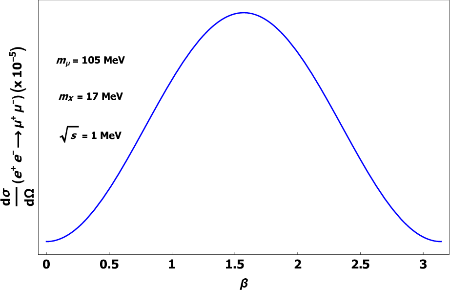
where $\beta$ is the scattering angle between the tri-momentum ${\bf p}$ and ${\bf p}^{\prime}$, or between ${\bf k}$ and ${\bf k}^{\prime}$ in the CM frame. We also consider $m_{e}\approx 0$ when compared to the muon mass $m_{\mu}=105.7\,\mbox{MeV}$. The result in Eq. (87) is illustrated in Figure 3 as a function of the $\beta$-angle.

References

• [1] A. J. Krasznahorkay et al, Phys. Rev. Lett. 116 (2016) 042501.
• [2] S. Weinberg, Phys. Rev. Lett. 40 (1978) 233.
• [3] L. B. Okun, Sov. Phys. JETP 56, 502 (1982).
• [4] B. Holdom, Phys. Lett. B 166, 196 (1986).
• [5] B. Holdom, Phys. Lett. B 178, 65 (1986).
• [6] P. Langacker, Rev. Mod. Phys., 2009, 81, 1199-1228.
• [7] P.-H. Gu , X.-G. He, Nuclear Physics B 919 (2017) 209-217.
• [8] J. L. Feng et al, Phys. Rev. Lett. 117 (2016) 071803.
• [9] T. Araki et al, Phys. Rev. D 95 (2017) 055006.
• [10] P. Fayet, Eur. Phys. J. C 77 (2017) 53.
• [11] U. Ellwanger and S. Moretti, JHEP (2016) 039.
• [12] C. W. Chiang and P. Y. Tseng, Phys. Lett. B 767 (2017) 289.
• [13] O. Seto and T. Shimomura, Phys. Rev. D 95 (2017) 095032.
• [14] Y. Kaneta and T. Shimomura, Prog. Theor. Exp. Phys. (2017) 053B04.
• [15] J. Kozaczuk et al, Phys. Rev. D 95, 115024 (2017).
• [16] Y. Kahn et al, JHEP 002, 05 (2017).
• [17] J. L. Feng et al, Phys. Rev. D 95 (2017) 035017.
• [18] M. Pospelov, Phys. Rev. D 80 (2009) 095002.
• [19] T. Kitahara and Y. Yamamoto, Phys. Rev. D 95 (2017) 015008.
• [20] M. Duerr and P. F. Perez, Phys. Lett. B 732 (2014) 101.
• [21] M. Duerr and P. F. Perez, Phys. Rev. D 91 (2015) 095001.
• [22] H. Davoudiasl, H.-S. Lee and W. J. Marciano, Phys. Rev. D 89 (2014) 095006.
• [23] J. Gulys et al, Nucl. Instrum. Methods Phys. Res., Sect. A 808, 21 (2016).
• [24] R. Barbieri and E. T. O. Ericson, Phys. Lett. B 57 (1975) 270.