General-Relativistic Dynamics of an Extreme Mass-Ratio Binary with an External Body
Abstract
We study the dynamics of a hierarchical three-body system in the general-relativistic regime: an extreme mass-ratio inner binary under the tidal influence of an external body. The inner binary consists of a central Schwarzschild black hole and a test body moving around it. We discuss three types of tidal effects on the orbit of the test body. First, the angular momentum of the inner binary precesses around the angular momentum of the outer binary. Second, the tidal field drives a “transient resonance” when the radial and azimuthal frequencies are commensurable. In contrast with resonances driven by the gravitational self-force, this tidal-driven resonance may boost the orbital angular momentum and eccentricity (a relativistic version of the Kozai-Lidov effect). Finally, as an orbit-dynamical effect during the non-resonant phase, we calculate the correction to the Innermost Stable Circular (mean) Orbit due to the tidal interaction. Hierarchical three-body systems are potential sources for future space-based gravitational wave missions and the tidal effects that we find could contribute significantly to their waveform.
I Introduction
The first direct detection of gravitational waves (GWs) [1] by ground-based detectors opens up a window to probe our universe, search for new physics and test the theory of General Relativity with unprecedented means. At the to frequency band, future space-based detectors such as the Laser Interferometer Space Antenna (LISA, see [2, 3]) will be able to observe signals from extreme mass-ratio inspirals (EMRIs) of massive black holes and stars/stellar-mass black holes, white dwarf binary mergers, etc. In particular, monitoring the orbital evolution of EMRIs offers a unique opportunity to probe the space-time of a rotating black hole (Kerr), as well as to improve our understanding of the dynamics of stars in galactic centres [4].
Because of the separation in mass-scales in EMRI systems, their dynamics can be modelled by black hole perturbation theory. Within this framework, the small expansion parameter is the ratio of the smaller mass to the larger mass, and the least massive object is approximated by a point mass. The two-body dynamics can thus be simplified to an effective one-body scenario, where a point mass moves on a geodesic of an ‘‘EMRI space-time” whose metric is the sum of the background metric due to the larger black hole and the (appropriately regularized) linear 11 1 Although here we only include the perturbation to first order in , that motion is geodesic on the “background+perturbation” space-time has been shown to second order in [21, 22]; it is expected that it holds to higher orders as well. gravitational perturbation generated by the smaller object. That is, the smaller object undergoes geodesic motion on this “background+perturbation” [5, 6]. In general, such trajectory is no longer geodesic on the background space-time, and the deviation is due to the metric perturbation induced by the smaller object itself, which give rise to a gravitational self-force [7]. Motivated by future space-based GW missions, understanding EMRI dynamics via the gravitational self-force has been one of the major efforts in gravitational physics in the past couple of decades.
If an EMRI system is not isolated, but is instead influenced by another massive astrophysical object, e.g., a supermassive black hole, the orbital dynamics and GW radiation are likely modified by the gravitational interaction between the inner binary and the third object. For instance, Yunes et al. [8] studied the acceleration of the EMRI system due to the gravitational attraction of the third body and they estimated the resulting phase variations in the gravitational waveform. On the other hand, even in the rest frame of the inner binary, the tidal field induced by the third body changes further the EMRI space-time. Such modification was first computed by Poisson [9] for the case of a non-rotating (Schwarzschild) central black hole and later on by Yunes and González [10] for the case of a Kerr black hole.
Understanding the dynamical influence of a tidal field on an EMRI orbit and waveform is the central goal of our work. As a first step along this path, we consider an extreme mass-ratio (inner) binary within an external tidal field under the following assumptions. We assume that the tidal field is created by a source which is slowly-moving around the inner binary (thus constituting an outer binary) and includes only the leading quadrupole moment (since the source is far from the inner binary). As for the inner binary, we assume that the central black hole is a Schwarzschild black hole and we ignore self-force effects (despite that we shall still refer to it as an EMRI).
Even with a Schwarzschild central black hole and ignoring self-force effects, we discover interesting and new effects due to the tidal field. Specificall, we investigate the following tidal-field effects on the orbit of the smaller particle. First, we show that the tidal field causes the angular momentum of the inner binary to precess around the angular momentum of the outer binary. This precession is caused by the interaction between quadrupole moment of the inner orbit and the tidal field. Second, we show that the tidal field leads to transient resonances: when the ratio of the (evolving) radial and angular orbital frequencies is a rational number, corrections larger than unity in the orbital phase may occur and the magnitude of the angular momentum may be boosted. Equivalent resonances have been observed within EMRI systems in the absence of a tidal field when including the dissipative piece of the self-force [11]. However, in contrast with our case, these self-force-driven resonances cannot increase the magnitude of the angular momentum (and can only occur when the central black hole is a Kerr black hole). Third and last, we calculate the shift, due to the tidal field, in the frequency, radius, energy and angular momentum of the Innermost Stable Circular Orbit (ISCO), which, for our system, we define in some orbital-average sense. Equivalent shifts have been found to be caused by the conservative piece of the self-force on particles moving around a Schwarzschild [12] or a Kerr [13] black hole. In our case, the frequency shift can be either positive or negative, as opposed to the self-force case which has been found to be positive.
The precession of angular momentum precession may lead to detectable GW phase variations within the precession timescales. The resonance effect could have significant observational imprints on the gravitational waveforms as we shall demonstrate later, which we expect to be true for generic Kerr-EMRI. The ISCO shift affects the peak frequency of the gravitational waveform, but we expect it to be small for the hierarchical triple systems considered here.
It is worth mentioning that in planetary systems, similar three-body dynamics have been extensively studied and many interesting behaviours have been discovered in the Newtonian and Post-Newtonian regimes For example, the well-known Kozai-Lidov (KL) mechanism [14, 15] suggests that the inner binary could trade eccentricity for inclination angle under the influence of the quadrupole tidal field of the third body. In recent years, the KL mechanism has been further extended to include eccentric orbits [16], the octupole tidal field [17, 18] and Post-Newtonian corrections [19, 20]. As the inner binary transfers from the Newtonian regime to the relativistic regime, the degeneracy between radial and angular orbital frequencies breaks down, which in principle allows for a much richer phenomenology, as indicated by previous Post-Newtonian studies [20]. To the best of our knowledge, the present work is the first study of the dynamics of such three-body systems in the fully relativistic regime.
I.1 An order-of-magnitude analysis
Before moving into a detailed analysis in later sections, we first present an order-of-magnitude estimate of the relative strength between the tidal field and the smaller object’s self-force. Such analysis may serve as an indication of the orbital modification generated by the tidal field during the gravitational radiation-reaction timescale. Throughout the paper we use units with .
Let us denote the inner binary orbit separation by and its two masses by and , with . The third body is at a distance and it has a mass . The system is illustrated in Fig.1.


The dynamics of the inner binary is influenced by: (i) the background spacetime of its MBH of mass ; (ii) the gravitational field of its smaller body of mass (; typically for EMRIs: ), causing a gravitational self-force [7, 21, 22, 5, 6]; (iii) the tidal force generated by the third body, another MBH of mass .
The dissipative part of the self-force is the driver of the secular change of the conserved quantities of the orbit of the EMRI system to . The self-acceleration is , where and are, respectively, the characteristic EMRI orbital separation and speed. The tidal acceleration is , where is the distance between and . As we show later, the orbital phase-shift generated by the tidal field during a transient resonance [11] is , whereas LISA’s phase resolution of a given event is (SNR: signal-to-noise ratio). Therefore, a tidal event is detectable if
| (1) |
with . We expect the tidal effect is easier to detect around the less massive MBH (), because its EMRI frequency is closer to the LISA band. Such orbits are also possibly eccentric due to the KL effect, in which case should be viewed as average radius and the peak frequency should be given by the periastron distance. According to [23], the detection rate of EMRIs by LISA ranges from a few tens to a few thousands per year, if the detection threshold of SNR is considered to be 22 2 The “average” SNR of detected events is higher than the detection threshold by definition, but it is not clear what are the exact values from [23]. Based on Monte-Carlo simulation of binary black holes for LIGO detections in a separate study [46], the distribution probability density of SNR roughly follows scaling, and hence the mean SNR of detected events is roughly times of detection threshold.. It is believed that tens of percent of Milky-Way-alike galaxies have experienced a MBH merger within the past Gyr [24, 25, 8]. For each merger, the time taken by the MBH binary to migrate to scale (through dynamical friction) is comparable to the local dynamical time of galaxies () [26], but the evolution from a distance of to (where GW radiation takes over) is still uncertain (this is known as the final parsec problem [27]). Taking the lifetime of MBH binaries to be several Gyr [26], it is possible that the decay time starting from a sub-parsec distance (Eq. (1)) is about several hundreds of million years (a few percent of Gyr). As a result, the optimal detection rate for the tidal effect by LISA is approximately a few .
We organize this paper as follows. In Sec. II we review Poisson’s [9] approach to calculating the deformation of the Schwarzschild metric due to the presence of an external tidal field. This approach will allow us to subsequently analyze the tidal effect in EMRI dynamics quantitatively. In Sec. III we show that the only secular effect by the tidal field outside a resonant phase is the precession of the orbital plane and we compute the precession frequency numerically. We also show in that section that during a resonance phase the rate of change of angular momentum may be nonzero. In Sec. IV we compute the shifts in the frequency, radius, energy and angular momentum of an orbital-averaged Innermost Stable Circular Orbit (ISCO) due to the tidal field. We conclude with a discussion in Sec.V.
II Formalism
Our physical setting is that of an EMRI system, composed of a small compact object and a massive black hole, within the influence of an external tidal field. The small compact object is modelled as a point test (i.e., the self-force is neglected) particle and it is moving around a massive black hole, which we shall take to be a Schwarzschild black hole. The tidal field is created by a third, remote and slowly-moving (in this paper we take the static limit over the period of inner binary) body; the tidal field is considered to be a perturbation of the metric of the massive black hole. Specifically, in our setting, is given by the Schwarzschild metric Eq.(5) below and the tidal perturbation will be given later in Eq.(11) combined with Eq.(13).
We may adopt two different but equivalent viewpoints to approach this problem. We note that these viewpoints apply similarly to the different setting of an EMRI system including the self-force but no external tidal field, in which case would correspond to the regularized gravitational self-field ( would continue to be the metric of the massive black hole).
In the first viewpoint, the smaller object is moving on an orbit of the background space-time and is undergoing an acceleration due to . The -acceleration is given by [7]
| (2) |
where is the -velocity of the particle, is the particle’s location (in a given system of coordinates ) and is the particle’s proper time. In principle, the -velocity in Eq.(2) should correspond to the accelerated orbit in . In practise, however, the -velocity in this accelerated orbit may be replaced with the -velocity of the geodesic (called the osculating geodesic) in which is instantaneously tangential to the accelerated orbit [28]. The reason is that the radiation-reaction timescale is much larger than the orbital timescale and the osculating geodesic agrees with the true accelerated orbit to zeroth order for small (corresponding to small in the case of the tidal force and to small in the case of the self-force). Therefore, using one velocity or the other in Eq.(2) only changes the force at higher-than-linear order in . When implementing Eq.(2) in this paper we shall use this osculating geodesic approximation. We shall use the symbol to denote any quantity which is conserved along geodesic motion in the space-time . Note that any such quantity is not necessarily conserved anymore when including the acceleration due to .
In the second viewpoint, the particle is considered to be following a geodesic of the full perturbed black hole space-time with metric . Within the Hamiltonian formalism (see, e.g., [29, 30] in the context of the conservative self-force), a particle’s geodesic motion in this space-time can be determined by invoking the Hamiltonian equations of motion. These equations are
| (3) |
where is the -momentum associated to the canonical position 33 3 In order to not overburden the notation we use the same symbol to denote the particle’s location in the two viewpoints, although strictly we should be differentiating between them since one is a location in and the other one in – it will be obvious from the context which one we mean. and is the particles’s proper time along the geodesic in . The Hamiltonian is given by
| (4) |
We shall use the symbol to denote any quantity which is conserved along geodesic motion in the perturbed space-time .
We shall essentially adopt the first viewpoint in the calculations from Sec.II.3 until Sec.IV, where, for convenience, we shall adopt the second viewpoint. The rest of this section is organized as follows. In Sec.II.1 we describe geodesic motion on a Schwarzschild black hole background . In Sec.II.2 we give expressions for a tidal perturbation . Finally, in Sec.II.3, we give expressions for rates of change of quantities which are conserved along geodesics in .
II.1 Geodesic motion on the black hole space-time
Here we consider geodesic motion on the black hole background space-time, i.e, with in Eq.(4).
In the case that the massive black hole is a Kerr black hole, particles following geodesic motion have three conserved quantities: the energy, , the component of the angular momentum along the spin (-)axis, , and the Carter constant [31]. Thanks to the three conserved quantities, the radial and angular geodesic motions are separable.
From now on, however, we restrict ourselves to the case that the massive black hole is a Schwarzschild black hole. The Schwarzschild line-element in Schwarzschild coordinates is
| (5) |
where and is the line-element of the -sphere. The same metric may be written in Ingoing-Eddington-Finkelstein coordinates as
| (6) |
where and is the tortoise radial coordinate.
Unlike in Kerr, in the Schwarzschild case the vector angular momentum is conserved, and the particle’s motion is planar. Because of the additional constraint of planar motion, there are only two effective degrees of freedom left. One of them is radial:
| (7) |
where we use “Mino time” , defined via , to parameterize the trajectory, following the discussion in [32]. We note that, in Schwarzschild, the Carter constant is given by and the square modulus of the total angular momentum is given by , for a given choice of Cartesian coordinates , and .
The motion along the -direction is given by
| (8) |
The motion along the -direction (for inclined orbits) can be obtained using a direct mapping from or, alternatively, from
| (9) |
The particle moves in the region , with being the angle between and the projection of onto the plane perpendicular to the -axis.
II.2 External tidal field
Poisson and collaborators [9, 33, 34] have obtained the metrics of black holes deformed by tidal forces which are created by a remote distribution of matter. They obtain these metrics by solving the perturbative Einstein equation and matching the solution to an external (asymptotic) tidal metric. In our case, we shall only take into account the leading – quadrupole – tidal moment of the field generated by the remote – third – body. This quadrupole moment can be characterized by electric-type tensors , and , and magnetic-type tensors and , where and are indices over the angular degrees of freedom and . These tensors can be obtained by decomposing the tidal field using tensor, vector and scalar spherical harmonics – their explicit definitions are given in [9, 33, 34]. As the outer object is only moving slowly, in this paper we shall neglect its motion over the orbital timescale of the inner binary. Hence, we shall take the magnetic-type tensor, as well as any derivatives of the electric-type tensor, to be zero in our analysis. Under these approximations of quadrupole moment and static source, the metric perturbation of a Schwarzschild black hole immersed in an external tidal field is:
| (10) |
For our purposes, it is more convenient to work with the metric perturbation in Schwarzschild coordinates, which is
| (11) |
The expressions in [9, 33, 34] for the electric-type (and magnetic-type) tensors are, in the static limit (within the dynamical timescale of the inner binary), in terms of an external gravitational potential , which can be expanded in multipoles. The dipole piece contributes to the acceleration of the center-of-mass of the inner binary as studied in [8]. Keeping only the quadrupole order terms, it is, trivially,
| (12) |
Here, is along the direction between the black hole of mass and the third body of mass , and its origin is at the location of ; is the polar angle with respect to the -axis. From the expressions in [9, 33, 34] for the electric-type tensors, it then follows that
| (13) |
II.3 Changes in “conserved quantities”
Let us now combine a background and a perturbation within the first viewpoint described at the start of this section. That is, we consider a particle in accelerated motion due to on a background . Then, the rate of change of a quantity , which is conserved along a geodesic in , may be obtained via
| (14) |
For example, let us find expressions for the rates of change of the energy, the angular momentum along the -direction and the Carter constant in the Schwarzschild background. These quantities in the case now of an accelerated orbit are still defined as in the case of a geodesic orbit in Sec.II.1, i.e., , and , respectively. Here, the correspond to the accelerated orbit but they are approximated by the values on the osculating geodesic. Eq. (14) then yields
| (15) |
The presence of a tidal field breaks the spherical symmetry of the background. Therefore, the tidal force is generically - or -dependent as well as -dependent. As a consequence, its secular effect implies averaging over one of these angular degrees of freedom as well as over the radial degree of freedom . That is, the Mino-time-averaged Mino-time-derivative of a quantity , which is conserved along the osculating geodesic in , is given by
| (16) |
or, equivalently, by
| (17) |
Here it is understood that in the integrands we write and, in Eq.(16), as functions of Mino time, as well as in Eq.(17). The “Mino time” periods in the - and -directions are, respectively, and
| (18) |
where is the minimum/maximum radius of the orbit. We note that corresponds to .
III Secular effects
The tidal-induced metric perturbation is stationary in time, which implies conservation of energy (of the orbit on when including tidal acceleration or, equivalently, of the geodesic on ), i.e., the rate of change of the total energy is zero – instantaneously and so also secularly. The rotational-symmetry along the line connecting the central black hole and the third body also implies conservation of angular momentum along that direction, , i.e., is conserved. We note that the relative difference between and is of order , which is expected to be small at all times. Therefore, we do not try to highlight their difference when studying secular evolution of the orbit unless it is necessary.
Now, consider a geodesic orbit in . By using the time-reversal symmetry of , one can argue that the secular rate of change of the magnitude of the total angular momentum of this orbit must be zero. The argument goes as follows. First, we notice that is a scalar that is invariant under the time-reversal operation. Secondly, because and are independent of time, a time-reversed trajectory still satisfies the correct equation of motion. Based on the above reasoning, if evolves from to after some period of time that is longer than the orbital timescale, a time-reversed orbit would evolve from to . Lastly, it is straightforward to see that an orbit is mapped to its time-reversed orbit under the reflection operation through a certain symmetry plane. The symmetry plane is that formed by the location of , the location of and the point on the orbit where
| (19) |
We argue that an orbit and its reflected one are identical in the sense that the points mapped to each other under reflection should carry the same , and consequently, must be the same as . The joint secular conservation of and then means that the opening angle, , between the orbital angular momentum and the symmetry axis of the tidal field must be invariant as well. As a result, the orbital angular momentum can only precess along the tidal symmetry axis (this is after orbit-averaging, not instantaneously), with a rate that we compute in Sec. III.1.
Let us now consider another secular effect due to the tidal field. For that purpose, we turn to the viewpoint where the orbit is accelerated in . We denote by , and the orbital frequencies (with respect to Mino time) associated to, respectively, the -, - and -motions of a geodesic in . A “transient resonance” is a point on the accelerated orbit such that the radial and angular frequencies of the osculating geodesic at that point are commensurate with each other: (there are only two independent frequencies in Schwarzschild, since the - and the -dynamics are degenerate and the motion is planar, so we could have equivalently used instead of in the condition), where and are prime numbers. In this case, the orbit becomes closed and the double integration in Eq. (16) or Eq. (17) reduces to an integral over the closed trajectory. The orbital-averaged rate of change of the magnitude of the angular momentum no longer vanish. We evaluate them and discuss their impact on the orbital phase in Sec. III.2.
III.1 Orbital Precession
Intuitively speaking, after averaging over the radial and angular (either azimuthal or polar) degrees of freedom, the particle trajectory occupies a finite-width ring ( between and ) in the orbital plane of the inner binary. We note that when we refer to any quantity (such as , , , etc) within this subsection, we shall in fact be refering to such orbital-average version of the quantity, even if we do not say so explicitly. The mentioned ring has minimum tidal potential energy , given in Eq.(12), if the orbital angular momentum is orthogonal to the tidal symmetry axis, and maximum energy if they are parallel. Therefore, a torque is exerted on the particle orbit, trying to tilt it to the minimum energy state. Such a torque generates precession of the orbital plane, in a similar way to the case of a top precessing under Earth’s gravitational field.
In this subsection we adopt the viewpoint of an accelerated orbit in . In order to evaluate the precession of the orbital plane due to the tidal interaction, we need to compute the secular rate of change of different components of the angular momentum. With of the choice of the -axis lying along the direction of the central black hole and the third body, must be conserved due to the symmetry argument above. The precession frequency (with respect to ) can be computed from the rate of change of and as:
| (20) |
where is the average lapse rate of with respect to [32]:
| (21) |
We evaluate the quantities in Eqs.(20) and (21) for the osculating geodesic and so, in particular, , and are constant. In order to evaluate the rate of change of and , we notice that
| (22) |
As a result, its rate of change is related to the acceleration by (as is conserved)
| (23) |
The rate of change of can be obtained similarly. Separately, one can compute the orbit-averaged interaction energy (based on the 2-D average of ) between the ‘‘mass ring” and the tidal field44 4 Similarly, Hamiltonian of the particle on a geodesic of is obtained later in Eq.(34). Such Hamiltonian contains a term that corresponds to the tidal interaction of the “mass ring”., which contains a term (with a proportionality factor independent of ), where is defined via the last equality as the angle between the tidal symmetry axis (here, parallel to ) and the orbital plane. Consequently, the modulus of the torque is equal to . Because the component of the angular momentum orthogonal to is proportional to , it must be
| (24) |
for a dimensionless function ; the proportionality factor measures the strength of the tidal-induced acceleration (see Eqs.(11) and (2)).
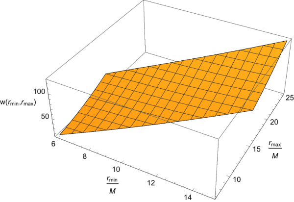
In Fig. 2, we present a calculation of , with a normalization constant to make it dimensionless and to remove the dependence on the strength of the tidal field. We have calculated in the following way. We have used Eq.(20), with and their derivatives calculated via Eqs.(22) and (23), via Eq.(2), from Eq.(11), and calculated by numerically integrating the geodesic equations in Schwarzschild. The (osculating) geodesic in the top panel corresponds to , and varying values of (equivalently, or ). This top panel confirms the dependence on given in Eq.(24), and the bottom panel gives the numerical value of . Apart from trajectories very close to the MBH, an approximate fit to Fig. 2 is , with .
The above calculation shows that, in principle, the angular momentum of the inner binary would in principle precess around the direction between the massive black hole and the third body . Now, assuming , an order-of-magnitude estimate for the period of the outer binary gives , which is generically much longer than the precession period: . Therefore, we also need to perform an average over the orbit of the third body. This can be done by writing down the equation for the precession of the angular momentum after averaging over the orbit of the inner binary, but allowing the direction of the third body () to be time-dependent. From Eq.(24) (for simplicity, here we do not distinguish between and ),
| (25) |
Let us assume that the motion of the third body is on some arbitrary – plane, so that we can write . The angular momentum of the outer binary is therefore perpendicular to the – plane and so parallel to the axis. By plugging this expression for into the above equation and averaging over an orbital period of the outer binary, , we obtain
| (26) |
Thus, now precesses around : Fig.1. Physically Eq. (25) and (26) describes the precession generated by the quadrupole moment-curvature coupling of the inner binary. For the MBH (outer) binary scenario considered here, the precession period is generically longer than the LISA observation timescale. However, we note that the precession effect also extends to the Newtonian regime as well as to comparable-mass binaries (instead of EMRIs). Thus, let us consider here –and only here– the case of stellar-mass BH binaries close to a MBH of mass , which could be relevant sources for both LISA and LIGO detections [35, 36, 37, 38, 39]. In this case, the precession period can be estimated as
| (27) |
where is taken to be for illustration purposes, is the GW frequency (twice the orbital frequency) of the stellar-mass binary and the component masses are assumed to be . Notice that such binaries (as well as EMRIs ) are likely to be eccentric due to the KL mechanism. Therefore, the waveform also contains a frequency component (where is the eccentricity) corresponding to the pericenter passage.
III.2 Resonance
In this subsection we consider a point in an accelerated orbit of the particle where the osculating geodesic (in ) is a resonant point. At a resonance, the osculating orbit is closed and we no longer consider “phase-space-averaged”-orbits which span a two-dimensional ring on a plane. In this sense, this situation is more similar to the Newtonian limit, which may be viewed as a resonance. In the Newtonian limit, the orbital eccentricity can be boosted to very high values via the Kozai-Lidov mechanism [14, 15]. Following the above analogy, we also expect a non-trivial change of eccentricity and angular momentum of the relativistic orbit during a resonance phase. In particular, the total angular momentum might be boosted, as compared to the monotonic reduction generated by the dissipative self-force 55 5 Note that the dissipative self-force may increase the eccentricity below a certain critical radius [47]..
In the calculation of the precession, an order-of-magnitude analysis showed that we could not neglect the orbit of the outer binary when . Let us carry out a similar order-of-magnitude analysis here. Also, the timescale of a transient resonance driven by the dissipative self-force generally scales as . By comparing it to the orbital timescale of the third body, we have . Therefore, for the case we study here, the static approximation for the tidal field applies.
In this subsection, we continue to choose the -axis to be parallel to the symmetry axis of the tidal field. Such setup is slightly different from the celestial coordinate setting in previous studies of hierarchical triple system in Newtonian and post-Newtonian regimes [16, 17, 20], as we do not perform the average over the third body’s orbit. On the other hand, our coordinate choice ensures rotational symmetry of the space-time around the -axis, so that must be conserved.
Suppose that , where and are coprime numbers. Then the integration of the rate of change of a quantity over a resonant closed orbit is
| (28) |
where . Such an integration is independent of the longitude of the ascending node for generic inclined orbits [40], but it does depend on the integration constant in the -motion,
| (29) |
which is related to the argument of the periastron [40]
In order to illustrate this point, we pick a resonance point with . This can be achieved with a one-parameter family of radius (e.g., either or ). For convenience, we choose and , although this choice is not unique. Also, we choose the inclination angle to be (). From Eqs.(28) and (15), with the tidal acceleration from Eqs.(2) and (11), we calculated the orbital-averaged rate of change of the Carter constant as a function of , for this chosen resonant orbit. We present this rate of change (which is trivially related to the corresponding rate of change of the total angular momentum ) in Fig.3. This plot clearly shows that the averaged rate of change of the Carter constant or, equivalently, of the total angular momentum, is nonzero during a resonance. In addition, the dependence on is well described by a sinusoidal function , as the pattern of the closed orbits repeats itself every -degree rotation in the argument of the periastron.
We performed a similar calculation of the averaged rates of change and and found that, as opposed to the calculation for , they are both zero (within the prescribed numerical accuracy of our calculation). The fact that the energy is conserved during a resonance phase due to the conservation of in the perturbed spacetime, and is consistent with previous studies in the Newtonian regime [40], although in that case averaging over the orbital phase has been applied to the third body, which is likely to have a longer period than the resonance crossing time in the systems that we are considering.
In general, might be boosted at a resonance, as opposed to the monotonic reduction generated by the dissipative self-force 66 6 Note that the dissipative self-force may increase the eccentricity below a certain critical radius [47].. This resonance effect due to the tidal force is in stark contrast with the case of the conservative self-force, which cannot drive resonances since it does not have an explicit -dependence [11]. Its existence also implies that the Newtonian KL effect and this relativistic KL effect might be formulated in a more general resonance kinetic theory framework. As Schwarzschild EMRIs are driven only by the dissipative self-force during a resonance, the shift of conserved quantities is and the resulting phase modification during the radiation-reaction timescale () is , which is much larger than unity. We have shown that tidal interaction also drives the evolution of conserved quantities during resonance. Its contribution to the phase error in the radiation-reaction timescale is . We emphasize that the secular amplification of order accumulates over the transient resonance scale. Therefore, this is an effect which cannot be captured by directly evaluating in the dynamical regime as in [8].
IV ISCO shift
As is well-known, the conservative piece of the gravitational self-force on the smaller mass in an EMRI system causes a shift in the ISCO frequency and radius, with respect to the test particle case [12, 13]. Similarly, in a hierarchical three-body system, the tidal field by the third body also modifies the ISCO frequency and radius of a Schwarzschild EMRI. In this section, we directly derive the shift in the ISCO frequency, radius, energy and angular momentum due to the tidal field, to leading order in . Therefore, while so far we have been considering general inspiral orbits, we now consider orbits which would be circular in the absence of the tidal field (similarly to the ISCO shift in the gravitational self-force case, where the orbits considered are those which would be circular in the absence of the dissipative self-force).
In this section, for the convenience of analysis and to allow easier implementation of previous results in the gravitational self-force problem, we choose a new coordinate system such that the -axis is orthogonal to the orbital plane of the inner binary (while it still goes through ). We shall also adopt the viewpoint that the particle is moving in a geodesic of the perturbed Schwarzschild space-time, similar to the treatment in [41, 13]. Correspondingly, the angles and are now the polar and azimuthal angle, respectively, with respect to this new -axis. Thus, in particular, the instantaneous angular velocity of the particle is given by .
Notice that the quantities for which we compute the ISCO shift are all gauge-dependent quantities (e.g., is conserved but gauge-dependent). Therefore, any result obtained here has to be associated with the gauge that we have chosen. This observation and the associated ambiguity has been emphasized in [42] in the context of the gravitational self-force problem. In that context, this issue is partly resolved by Detweiler in [41] by considering quantities (such as ) which, on “quasi-circular” orbits are pseudo-invariants with respect to helical-symmetric gauge transformations:
| (30) |
where is the Lie-derivative with respect to the helical symmetry vector . In our case, however, the external field itself breaks such symmetry, and it is not clear whether there is a similar construction of pseudo-invariant quantities. On the other hand, it is possible to assert an angular-averaged version of helical symmetry:
| (31) |
If the above requirement is satisfied, it is straight-forward to modify Detweiler’s derivation of gauge invariance of to prove the invariance of on “quasi-circular” orbits with respect to any gauge choices satisfying Eq. (31). Note that, based on Eqs. (8) and (9), the average over can be replaced by an average over a period of .
There is one more restriction on the gauge choice, though a rather natural one. Detweiler requires the gravitational perturbation not only to respect the helical symmetry Eq.(30) but also the reflection symmetry through the equatorial plane. The tidal field in our system, however, leads to the violation of this symmetry. If one does not require reflection symmetry, the changes in the metric perturbation under a gauge transformation are then given by those in Eqs.B2-B7 [41] with the only following modification:
| (32) |
where is the gauge vector. Because here we are considering orbits on the equatorial plane (where ), the modification term in Eq.(32) vanishes as long as is finite. As a result, the gauge-invariance of is mantained under gauge transformations that preserve Eq.(31) and with finite.
Because the tidal field breaks the axi-symmetry when the orbital angular momentum is not aligned with the symmetry axis of the tidal field, there is no innermost orbit with strictly circular motion (in fact, there are no strictly-circular orbits at all). Instead, the true trajectory (on the full metric ) has a slight oscillation in the radial coordinate of magnitude . In fact, if for a moment we take the point of view that the particle is moving in an accelerated orbit in Schwarzschild space-time, the tidal forces (proportional to ) in both radial and azimuthal angle directions contain pieces that are periodic in and pieces that are independent of . By solving the equations of motion including the tidal acceleration, it is easy to see that the radial motion of the ISCO orbit (note that the orbit is not actually circular, but it is an innermost stable, circular mean orbit) can be written as for some , where () are coefficients independent of . Such description should also be valid in the perturbed space-time picture to which we now return, i.e., the orbit is closed to leading order in . Given a Hamiltonian of the “EMRI+tidal interaction system”, we define as a dimensionless quantity. Let us denote by the “mean” circular orbit (on ) with radius . We notice that is not strictly geodesic and that it has a Hamiltonian order away from the true trajectory 77 7 A similar treatment was employed in [13] to compute the ISCO shift on the equator of Kerr due to the gravitational self-force.. In other words, the effect of radial motion only contributes with terms to the Hamiltonian. As a result, we can replace with the mean circular trajectory , which is convenient for practical calculations. Accordingly, we calculate , where we define the ISCO-orbital-average of a quantity as
| (33) |
where is evaluated along . In the case of , we obtain it from Eq.(4), using Eqs.(11) and (13) and setting , and (where is with respect to the new -axis). The resulting, dimensionless and averaged, Hamiltonian is
| (34) |
The ISCO condition now reduces to (without distinguishing from here and by adopting the argument in [13]):
| (35) |
Let us define . Then, when including the tidal field, the energy, angular momentum, radius and orbital frequency at the mean orbit of ISCO are, given by, respectively,
| (36) |
where , , and are the values for a test particle on the ISCO in Schwarzschild and , , and are defined with respect to their expansion order in . By plugging Eq.(36) into Eq. (35) we obtain the following shifts:
| (37) |
The ISCO frequency in the perturbed space-time is given by [41] and we apply it on the mean circular orbit of ISCO (i.e., ):
| (38) |
In order to evaluate this expression, we need the following orbital-averages, which are readily obtained:
| (39) |
V Discussion and Conclusion
We have performed an analysis of the general-relativistic dynamics of a Schwarzschild EMRI (without gravitational self-force) residing in an external quadrupole tidal field. As discussed earlier, the detection rates of such systems are still subject to uncertainties in EMRI merger rate as well as the merger history of MBHs before GW radiation takes over. This also means that a possible detection of such event would also shed light on the myth of the MBH merger mechanism. It would also provide a unique opportunity to test a perturbed Schwarzschild/Kerr metric predicted by General Relativity, as it has distinctive dynamic and waveform features compared to isolated EMRI systems.
We have discussed three interesting relativistic effect due to the tidal interactions. First, in the non-resonant phase of the EMRI orbit, the main secular effect of this tidal interaction is the precession of the orbital plane around the orbital angular momentum of the outer binary. This precession may contribute at order to the phase of the waveform during the precession timescale, given by . However, such precession timescale for EMRIs might be longer than observation timescale of LISA, whereas a similar mechanism applied to stellar mass binary systems near a SMBH gives precession timescale in the LISA band. Second, during the resonant phase, the magnitude of the angular momentum may increase or decrease, in stark comparison with the monotonic suppression driven by the dissipative part of the self-force. The fractional change in the magnitude of the angular momentum driven by the tidal-field during a resonance is, when including the dissipative self-force as well as the tidal force, proportional to , and the resulting orbital phase modification is . This value could be greater than phase resolution of LISA depending on the strength of the tidal field and the parameters of the inner binary. Finally, in order to capture some of the dynamical effects due to the tidal field, we also included a calculation of the shift in frequency, radius, energy and angular momentum of the ISCO. In contrast with the conservative piece of the gravitational self-force, which always causes a positive frequency shift in Schwarzschild [12] and for all spins sampled in Kerr [13], the tidal field could lead to either a positive or a negative ISCO frequency shift, depending on the inclination angle of the orbit. In particular, orbits with undergo a negative frequency shift, while orbits with undergo a positive frequency shift. A negative frequency shift corresponds to an earlier merger, and a positive frequency shift to a later merger.
To the best of our knowledge, our analysis is the first fully-relativistic one of three-body systems. In the future, it will be interesting to extend our analysis to the cases of a central Kerr black hole and of inclusion of the gravitational self-force. In addition, for planetary systems it has been shown that octupole-order tidal field by the third body could generate much richer dynamics [17, 18]. For the system we consider here, tidal effect affects the GW waveform mostly through transient resonance phases. During such limited evolution within transient resonances, as the magnitude of octupole order tidal force is smaller than the quadrupole order tidal force, it should be subdominant unless we are dealing with highly-eccentric orbits.
Finally, we note that we have analyzed the case where the inner binary is in the extreme mass-ratio regime. It is reasonable to expect that the analytical understanding that we have provided could shed some light on the dynamics of triple systems with a comparable-mass (stellar mass) inner binary, similarly to the spirit of using the Effective-One-Body formalism for describing the nonlinear two-body problem [43]. Such triple systems could form in nuclear field clusters and they are expected to be important sources for ground-based GW detectors [35, 36, 37, 38, 44, 45].
Acknowledgements- H.Y. thanks Scott Hughes for valuable discussions and comments, as well as Scott Tremaine and Chiara Mingarelli for information on evolution history of MBH binaries. M.C. acknowledges partial financial support by CNPq (Brazil), process number 308556/2014-3. The authors thank anonymous referees for interesting discussions and many helpful comments.
References
- [1] B. P. Abbott, R. Abbott, T. D. Abbott, M. R. Abernathy, F. Acernese, K. Ackley, C. Adams, T. Adams, P. Addesso, R. X. Adhikari, et al. (LIGO Scientific Collaboration and Virgo Collaboration), Phys. Rev. Lett. 116, 061102 (2016), URL http://link.aps.org/doi/10.1103/PhysRevLett.116.061102.
- [2] P. Amaro-Seoane, S. Aoudia, S. Babak, P. Binétruy, E. Berti, A. Bohé, C. Caprini, M. Colpi, N. J. Cornish, K. Danzmann, et al., Classical and Quantum Gravity 29, 124016 (2012), URL http://stacks.iop.org/0264-9381/29/i=12/a=124016.
- [3] Prince, T. A., Binetruy, P., Centrella, J., Finn, L. S., Hogan, C. and Nelemans, G., Phinney, E. S., Schutz, B. and LISA International Science Team, Tech. Rep., LISA science case document (2007), available as http://list.caltech.edu/mission_documents.
- [4] P. Amaro-Seoane, B. Schutz, and N. Yunes, arXiv preprint arXiv:1003.5553 (2010).
- [5] S. Detweiler and B. F. Whiting, Phys. Rev. D 67, 024025 (2003).
- [6] S. Detweiler, Phys. Rev. Lett. 86, 1931 (2001), URL http://link.aps.org/doi/10.1103/PhysRevLett.86.1931.
- [7] E. Poisson, A. Pound, and I. Vega, Living Rev. Rel. 14, 7 (2011).
- [8] N. Yunes, M. Coleman Miller, and J. Thornburg, Phys. Rev. D 83, 044030 (2011), URL http://link.aps.org/doi/10.1103/PhysRevD.83.044030.
- [9] E. Poisson, Phys. Rev. Lett. 94, 161103 (2005), URL http://link.aps.org/doi/10.1103/PhysRevLett.94.161103.
- [10] N. Yunes and J. A. González, Phys. Rev. D 73, 024010 (2006), URL http://link.aps.org/doi/10.1103/PhysRevD.73.024010.
- [11] E. E. Flanagan and T. Hinderer, Phys. Rev. Lett. 109, 071102 (2012).
- [12] L. Barack and N. Sago, Phys. Rev. Lett. 102, 191101 (2009), eprint 0902.0573.
- [13] S. Isoyama, L. Barack, S. R. Dolan, A. Le Tiec, H. Nakano, A. G. Shah, T. Tanaka, and N. Warburton, Phys. Rev. Lett. 113, 161101 (2014).
- [14] Y. Kozai, The Astronomical Journal 67, 591 (1962).
- [15] M. Lidov, Planetary and Space Science 9, 719 (1962).
- [16] Y. Lithwick and S. Naoz, The Astrophysical Journal 742, 94 (2011).
- [17] G. Li, S. Naoz, B. Kocsis, and A. Loeb, Monthly Notices of the Royal Astronomical Society 451, 1341 (2015).
- [18] B. Katz, S. Dong, and R. Malhotra, Physical Review Letters 107, 181101 (2011).
- [19] C. M. Will, Classical and Quantum Gravity 31, 244001 (2014), URL http://stacks.iop.org/0264-9381/31/i=24/a=244001.
- [20] S. Naoz, B. Kocsis, A. Loeb, and N. Yunes, The Astrophysical Journal 773, 187 (2013a).
- [21] A. Pound, Phys. Rev. Lett. 109, 051101 (2012).
- [22] S. E. Gralla, Phys. Rev. D 85, 124011 (2012).
- [23] J. R. Gair, S. Babak, A. Sesana, P. Amaro-Seoane, E. Barausse, C. P. Berry, E. Berti, and C. Sopuerta, arXiv preprint arXiv:1704.00009 (2017).
- [24] E. F. Bell, S. Phleps, R. S. Somerville, C. Wolf, A. Borch, and K. Meisenheimer, The Astrophysical Journal 652, 270 (2006).
- [25] J. M. Lotz, M. Davis, S. Faber, P. Guhathakurta, S. Gwyn, J. Huang, D. Koo, E. Le Floc?h, L. Lin, J. Newman, et al., The Astrophysical Journal 672, 177 (2008).
- [26] L. Z. Kelley, L. Blecha, and L. Hernquist, Monthly Notices of the Royal Astronomical Society 464, 3131 (2017).
- [27] M. Milosavljević and D. Merritt, The Astrophysical Journal 596, 860 (2003).
- [28] A. Pound and E. Poisson, Phys. Rev. D 77, 044013 (2008).
- [29] J. Vines and É. É. Flanagan, Phys. Rev. D 92, 064039 (2015).
- [30] R. Fujita, S. Isoyama, A. L. Tiec, H. Nakano, N. Sago, and T. Tanaka, arXiv preprint arXiv:1612.02504 (2016).
- [31] B. Carter, Phys. Rev. 174, 1559 (1968).
- [32] S. Drasco, E. E. Flanagan, and S. A. Hughes, Classical and Quantum Gravity 22, S801 (2005).
- [33] E. Poisson and I. Vlasov, Phys. Rev. D 81, 024029 (2010), URL http://link.aps.org/doi/10.1103/PhysRevD.81.024029.
- [34] E. Poisson, Phys. Rev. D 91, 044004 (2015).
- [35] F. Antonini and H. B. Perets, The Astrophysical Journal 757, 27 (2012).
- [36] T. A. Thompson, The Astrophysical Journal 741, 82 (2011).
- [37] F. Antonini, N. Murray, and S. Mikkola, The Astrophysical Journal 781, 45 (2014).
- [38] K. Silsbee and S. Tremaine, arXiv preprint arXiv:1608.07642 (2016).
- [39] J. H. VanLandingham, M. C. Miller, D. P. Hamilton, and D. C. Richardson, The Astrophysical Journal 828, 77 (2016).
- [40] S. Naoz, W. M. Farr, Y. Lithwick, F. A. Rasio, and J. Teyssandier, Monthly Notices of the Royal Astronomical Society p. stt302 (2013b).
- [41] S. Detweiler, Phys. Rev. D 77, 124026 (2008).
- [42] L. Barack and A. Ori, Phys. Rev. D 64, 124003 (2001).
- [43] A. Buonanno and T. Damour, Phys. Rev. D 59, 084006 (1999), URL https://link.aps.org/doi/10.1103/PhysRevD.59.084006.
- [44] Y. Meiron, B. Kocsis, and A. Loeb, The Astrophysical Journal 834, 200 (2017), URL http://stacks.iop.org/0004-637X/834/i=2/a=200.
- [45] L. Wen, The Astrophysical Journal 598, 419 (2003).
- [46] H. Yang, K. Yagi, J. Blackman, L. Lehner, V. Paschalidis, F. Pretorius, and N. Yunes, Physical Review Letters 118, 161101 (2017).
- [47] T. Apostolatos, D. Kennefick, A. Ori, and E. Poisson, Phys. Rev. D 47, 5376 (1993), URL http://link.aps.org/doi/10.1103/PhysRevD.47.5376.