Power-and Rate-Adaptation Improves the Effective Capacity of C-RAN for Nakagami- Fading Channels
Abstract
We propose a power-and rate-adaptation scheme for cloud radio access networks (C-RANs), where each radio remote head (RRH) is connected to the baseband unit (BBU) pool through optical links. The RRHs jointly support the users by efficiently exploiting the enhanced spatial degrees of freedom. Our proposed scheme aims for maximizing the effective capacity (EC) of the user subject to both per-RRH average-and peak-power constraints, where the EC is defined as the maximum arrival rate that can be supported by the C-RAN under the statistical delay requirement. We first transform the EC maximization problem into an equivalent convex optimization problem. By using the Lagrange dual decomposition method and solving the Karush-Kuhn-Tucker (KKT) equations, the optimal transmission power of each RRH can be obtained in closed-form. Furthermore, an online tracking method is provided for approximating the average power of each RRH. For the special case of two RRHs, the expression of the average power of each RRH can be calculated in explicit form. Hence, the Lagrange dual variables can be computed in advance in this special case. Furthermore, we derive the power allocation for two important extreme cases: 1) no delay constraint; 2) extremely stringent delay-requirements. Our simulation results show that the proposed scheme significantly outperforms the conventional algorithm without considering the delay requirements. Furthermore, when appropriately tuning the value of the delay exponent, our proposed algorithm is capable of guaranteeing a delay outage probability below when the maximum tolerable delay is 1 ms. This is suitable for the future ultra-reliable low latency communications (URLLC).
I Introduction
The fifth-generation (5G) wireless system to be deployed by 2020 is expected to offer a substantially increased capacity [1]. To achieve this ambitious goal, the C-RAN concept has been regarded as one of the most promising solutions. In particular, C-RAN is composed of three key components: 1) a pool of BBUs centrally located at a cloud data center; 2) low-cost, low-power distributed RRHs deployed in the network; 3) high-bandwidth low latency fronthaul links that connect the RRHs to the BBU pool. Under the C-RAN architecture, most of the baseband signal processing of conventional base stations has been shifted to the BBU pool and the RRHs are only responsible for simple transmission/reception functions, some of the hitherto centralized signal processing operations can be relegated to the BBU pool. Hence, the network capacity can be significantly improved.
Recently, the performance of C-RAN has been extensively studied [2, 3, 4, 5], albeit these papers have been focused on the physical layer issues, which giving no cognizance to the delay of the upper layer’s. However, most of the multimedia services, such as video conferencing and mobile TV have stringent delay requirements. Due to the time-varying characteristics of fading channels, it is impossible to impose a deterministic delay-bound guarantee for wireless communications. For the sake of analyzing the statistical QoS performance, Wu et al. [6] introduced the notion of effective capacity (EC), which can be interpreted as the maximum constant packet arrival rate that can be supported by the system, whilst satisfying a maximum buffer-violation probability constraint.
Due to the complex expression of EC, most of the existing papers focus on the EC maximization problem for the simple scenario, where there is only a single transmitter [7, 8, 9, 10, 11]. Specifically, a QoS-driven power-and rate-adaptation scheme was proposed for single-input single-output (SISO) systems communicating over flat-fading channels in [7], with the objective of maximizing EC subject to both delay-QoS and average power constraints, which is characterized by the QoS exponent . A smaller corresponds to a looser QoS guarantee, while a higher value of represents a more stringent QoS requirement. The results of [7] showed that in the extreme case of , the power allocation reduces to the conventional water-filling solution. By contrast, when , the optimal power allocation becomes the channel inversion scheme, where the system operates under a fixed transmission rate. The EC maximization problem was studied in [8] in the context of cognitive radio networks, where the power constraints of [7] were replaced by the maximum tolerable interference-power at the primary user. Closed-form expressions of both the power allocation and the EC were derived for the secondary user. The power minimization problem subject to EC constraints was considered in [9] for three different scenarios. Significant power savings can be achieved by using the power allocation scheme of [9]. To a further advance, both subcarrier and power allocation were investigated in [10] for a one-way relay network wherein the optimal subcarrier and power allocation was derived by adopting the Lagrangian dual decomposition method. Most recently, Wenchi et al. [11] considered both the average-and peak-power constraints when maximizing the EC, and provided the specific conditions, when the peak power constraints can be removed. From the information-theoretical point of view, it is difficult to solve the ergodic capacity maximization problem subject to both the average-and peak-power constraints, even for the basic Gaussian white noise channel. In Shannon’s landmark paper [12], only the asymptotically low and high SNR for the bandlimited continuous time Gaussian channel was studied. This problem was later studied by Smith [13] and showed that the capacity achieving distribution is discrete. In [14], the authors considered the more general case of the quadrature additive Gaussian channel and derived the lower and upper bounds of this channel’s capacity. Khojastepour et al. [15] studied the capacity of the fading channel under both types of power constraints under the assumption of the perfect channel state information available at both the transmitter and receiver side. However, the above papers [12, 13, 14] neither consider the upper layer delay nor the multiple transmission points.
To avoid any traffic congestion and attain a good C-RAN performance, the adaptive power allocation scheme should take the diverse QoS requirements into account to guarantee the satisfaction of users. In this paper, we aim for jointly optimizing the power allocation of each RRH in order to maximize the EC of a user of the C-RAN, where both the average power and peak power constraints of each RRH are considered. This user is jointly served by all RRHs of the C-RAN due to the powerful computational capability of the BBU pool. Unfortunately, the power allocation schemes developed in the aforementioned papers for single-transmitter scenarios [7, 8, 9, 10, 11] cannot be directly applied to C-RAN’s relying on multiple RRHs for serving the user and to simultaneously exploit the spatial degrees of freedom. The reason can be explained as follows. In these papers, there is only a single transmitter and only a sum-power constraint is imposed. The Lagrange method can be used to find the optimal power allocation, which is in the form of a water-filling-like solution in general. However, for the C-RAN, all RRHs have their individual power constraints and the power cannot be shared among the RRHs. Yu et al. [16] provided a detailed reason as to why the classic Lagrange method cannot be readily applied in C-RAN. Hence, new methods have to be developed. Specifically, the contributions of this paper can be summarized as follows:
- 1.
In this paper, we derive the optimal power allocation for each RRH by resorting to the Lagrangian dual decomposition and the Karush-Kuhn-Tucker (KKT) conditions. The power allocation solutions depend both on the user’s QoS requirements and on the joint channel conditions of the RRHs.
- 2.
The Lagrangian dual decomposition requires us to calculate the subgradient, where the average power of each iteration should be obtained. However, it is numerically challenging to derive the expression of average power for each RRH. To tackle this issue, we provide an online training method for tracking the average power of each RRH. For the special case of a single RRH, the closed-form expression of average power can be obtained. For the more complex case of two RRHs, we also provide the expression of the average power for each RRH in explicit form, which can be numerically evaluated.
- 3.
We provide the closed-form power allocation solutions for two extremely important cases: 1) When the QoS exponent approaches zero, which corresponds to the conventional ergodic capacity maximization problem; 2) When the QoS exponent tends to infinity, which represents the strictly delay-limited case. We also extend our work to the more general multiuser case, where the optimal transmit power for each user is derived.
- 4.
Our simulation results will show that the proposed algorithms significantly outperforms the existing algorithms. Additionally, by appropriately choosing the QoS exponent, our proposed delay-aware algorithm can guarantee a delay-outage probability below , when the maximum tolerable end-to-end (E2E) delay is 1 ms, which satisfies the strict delay requirements of the future ultra-reliable low latency communications (URLLC).
The most closely related paper of our work is [11], where single transmitter is considered. The optimal power allocation can be readily derived in closed form by the aid of the Lagrangian dual decomposition, which is in the water-filling-like form. However, our considered C-RAN involves multiple independent transmitters, the power allocation derivations are much more involved, and the power allocation solution is not the same as the conventional water-filling form. In [11], only one dual variable needs to be optimized, which can be obtained by using the bisection search method, while multiple dual variables are involved in the C-RAN scenario and the subgradient method is adopted to update the dual variables. Furthermore, in both papers, the average power expression is required in the updating of dual variables. However, this issue is not studied in [11], while our paper provides more details about the analysis of this issue.
| The number of RRHs | |
|---|---|
| The set of RRHs | |
| The time frame length | |
| Nakagami parameter | |
| Channel-power-to-noise ratio (CPNR) | |
| QoS exponent | |
| The effective capacity specified by | |
| Constant arrival data rate | |
| Maximum delay bound | |
| System bandwidth | |
| Average power constraint of RRH | |
| Peak power constraint of RRH |
The rest of this paper is organized as follows. In Section II, the C-RAN system is introduced along with the concept of EC and our problem formulation. In Section III, we provide the optimal power allocation for the general case of any number of RRHs. In Section IV, we derive the integral expressions’s closed-form solution concerning the average transmit power of each RRH for the sake of updating the Lagrangian dual variables. In Section V, we obtain the power allocation for two extreme cases, namely for the delay-tolerant scenario and for extremely stringent delay constraints. Numerical results are also provided in Section VII. Finally, our conclusions are drawn in Section VIII. The other notations are summarized in Table. I.
II system model
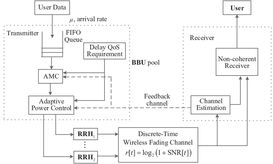
Consider a downlink C-RAN consisting of RRHs and a single user 11 1 The method developed in this paper can also be applied to the multi-user scenario, where all users apply the classical orthogonal frequency division multiplexing access (OFDMA) technique to remove the multi-user interference., where each RRH and the user have a single antenna, as depicted in Fig. 1. The set of RRHs is denoted as . All the RRHs are assumed to be connected to the BBU pool through the fronthaul links relying on high-speed fiber-optic cables. In Fig. 2, the upper layer packets are first buffered in first-in-first-out (FIFO) queue, which will be transmitted to the physical layer of the RRHs. Since the RRHs are only responsible for simple transmission/reception, we do not consider the storage function at the RRHs. At the data-link layer, the upper-layer packets are partitioned into frames and then each frame will be mapped into bit-streams at the physical layer. The channel is assumed to obey the stationary block fading model, implying that they are fixed during each time frame of length of , while it is switched independently over different time frames.
To elaborate, we consider a Nakagami- block-fading channel, which is very general and includes most of the practical wireless communication channels as special cases[17]. The parameter represents the severeness of the channel, where the fading channel fluctuations are reduced with . The probability density function (PDF) of the Nakagami- channel spanning from the -th RRH to the user is given by:
| (1) |
where is the Gamma function, denotes the instantaneous channel-power-to-noise ratio (CPNR) from the th RRH to the user, and is the average received CPNR at the user from the th RRH, denoted as , where is the large-scale fading channel gain spanning from the th RRH to the user that includes the path loss and shadowing effect, and is the noise power.
Let us define . Since are independent, the joint PDF of is given by
| (2) |

II-A Effective Capacity (EC)
This paper considers the E2E delay requirement for each packet. In C-RANs, the E2E delay, denoted as , includes the uplink (UL) and downlink (DL) transmission delays of , queueing delay at the buffer of the BBU pool of , and the fronthaul delay of . Since the fronthaul links are usually deployed with high-speed fiber, the fronthaul delay is much less than 1 ms [18]. In addition, since the packet size in URLLC is very short, the UL and DL transmission can be finished within a very short time. Hence, the E2E delay is mainly dominated by the queueing delay at the buffer of the BBU pool, which is given by . In the following, we mainly focus on the study of the queueing delay, which is characterized by the EC.
The EC is defined as the maximum constant frame arrival rate that a given service process can support, while obeying the delay requirement indicated by the QoS exponent that will be detailed later. Let the sequence represent the data service-rate, which follows a discrete-time stationary and ergodic stochastic process. The parameter is the time frame index. Let us denote by the partial sum of the service process over the time sequence spanning from to . Let us furthermore assume that the Gartner-Ellis limit of , which is denoted by , is a convex differentiable function for all real-value of [7]. Then, the EC of the service process specified by is
| (3) |
where denotes the expectation operator.
Let us assume that a data source enters a queue of infinite buffer size at a constant data rate . The probability that the delay exceeds a maximum delay bound of satisfies [6]
| (4) |
where indicates that , and is the probability that the buffer is non-empty, which can be calculated by using the method in [6]. The parameter can be found by letting the constant arrival rate to be equal to the EC, i.e. setting it to . Hence, if the delay-bound violation probability is required to be below , one should limit its incoming data rate to a maximum of .
It is seen from (4) that is an important parameter, representing the decay rate of the delay violation probability. A smaller corresponds to a slower decay rate, which indicates that the delay requirement is loose, while a larger corresponds to a faster decay rate, which implies that the system is capable of supporting a more stringent delay requirement. In other words, when , an arbitrarily long delay can be tolerated by the system, which corresponds to the capacity studied in Shannon information theory. On the other hand, when , this implies that no delay is allowed by the system, which corresponds to the very stringent statistical delay-bound QoS constraint of allowing no delay at all.
II-B Problem formulation
For the user, we assume that the non-coherent joint transmission is adopted as the BBU pool [19, 20, 21]. Then, the instantaneous service rate of a single frame, denoted by , can be expressed as follows [22, 23]:
| (5) |
where is the system’s bandwidth, represents the network condition that includes both the channel’s power gains and the EC exponent requirement, and represents the power allocation for RRH that depends on the network’s condition . In this paper, we aim for optimizing the transmit power in order to maximize the EC for the user under two different types of power limitations for each RRH: under an average power constraint and a peak power constraint. The first one is related to the long-term power budget, while the second guarantees that the instantaneous transmit power is below the linear range of practical power amplifiers. Mathematically, this optimization problem can be formulated as
| (6a) | ||||
| (6b) | ||||
| (6c) | ||||
where denotes the expectation over , while and denote the th RRH’s maximum average transmit power constraint and peak transmit power constraint, respectively.
III Optimal Power Allocation Method
By exploiting the fact that is a monotonically increasing function, Problem (6) can be equivalently simplified as
| (7a) | ||||
| (7b) | ||||
| (7c) | ||||
where we have . In Appendix A, we prove that Problem (7) is a convex optimization problem. Hence, the Lagrangian duality method can be used to solve Problem (7) with zero optimality gap.
Note that in Problem (7), only the average power constraints are ergodic, while the others are instantaneous power constraints. Similar to [24], we should first introduce the dual variables associated with the average transmit power constraints. Then, the original problem can be decomposed into several independent subproblems, where each one corresponds to one fading state. In addition, the instantaneous power constraints are enforced for each fading state. Let represent the nonnegative dual variables associated with the average power constraints. The Lagrangian function of Problem (7) can be written as
| (8) | |||||
where . Let us now define . The Lagrange dual function is then given by
| (9) |
The dual problem is defined as
| (10) |
As proven in Appendix A, Problem (7) is a convex optimization problem, which implies that there is no duality gap between the dual problem and the original problem. Thus, solving the dual problem is equivalent to solving the original problem.
To solve the dual problem in (10), we should solve the problem in (9) for a fixed , then update the Lagrangian dual variables by solving the dual problem in (10). Iterate the above two steps until convergence is reached.
1) Solving the dual function in (9): For a given , we should find the dual function , which can be rewritten as
| (11) |
where we have:
| (12) |
Note that can be decoupled into multiple independent subproblems, each corresponding to a specific fading state. Those subproblems have the same structure for each fading state. Hence, to simplify the derivation, is omitted in the following. Each subproblem can be expressed as:
| (13a) | ||||
| s.t. | (13b) | |||
The above problem is convex. In the following, we obtain the closed-form solution by solving the KKT conditions of Problem (13).
First, we introduce the nonnegative dual variables of , and for the associated constraints in (13b). The KKT conditions for Problem (13) can be expressed as
| (14a) | |||
| (14b) | |||
| (14c) | |||
| (14d) | |||
| (14e) | |||
with , , and , . Then, we have the following lemma.
Lemma 1: For any two arbitrary RRHs and , if and , then the following relationship must hold
| (15) |
Proof: Please see Appendix B.
Lemma 1 shows that the RRHs associated with a smaller should be assigned a non-zero power, while the RRHs having a larger value should remain silent. Let us hence introduce as a permutation over , so that we have , when . Let be the set of RRHs that transmit at a non-zero power. Then, according to Lemma 1, it can be readily verified that we have .
Lemma 2: There is at most one RRH associated with , and the RRH index is .
Proof: Please see Appendix C.
Next, we derive the optimal power allocation of Problem (13) shown as in Theorem 1.
Theorem 1: The optimal solution of Problem (13) is shown as follows,
| (16) |
where is given by
with being the largest value of integer , so that we have
| (17) |
Proof: Please refer to Appendix D.
It can be seen from (16) that the RRHs with high value of should be switched off, and the ones with larger values can transmit with peak power. The dual variable can be regarded as the price, and larger value of will incur higher cost when the RRH is active.
Corollary 1: When the number of RRHs is equal to one, i.e. , the optimal transmit power is given by
| (18) |
where is given by
Proof: It is can be readily derived using Theorem 1.
Note that the above result is consistent with the point-to-point result obtained in [11].
2) Solving the dual problem (10): To solve the dual problem (10), we invoke the subgradient method, which is a simple method of optimizing non-differentiable objective function [25]. The subgradient is required by the subgradient of at in the th iteration22 2 According to [25], a vector is a subgradient of at , if for all , holds..
Theorem 2: The subgradient of at in the th iteration is given by
| (19) |
where is the optimal solution of Problem (9) when we have , and .
Proof: Please see Appendix E.
Based on Theorem 2, the Lagrangian dual variables can be updated as
| (20) |
where is the step in the iteration. The subgradient method is guaranteed to converge if satisfies and [26]. The step size in the simulation section is set as , where is the constant step-size parameter.
In summary, the solution of Problem (6) is given in Algorithm 1.
To execute Algorithm 1, there is another issue that has to be tackled, namely how to calculate the average power for each RRH in order to obtain the subgradient . Given the dual variables , the expression of optimal power at each RRH depends on the generations of channel gains . Different generations of will lead to different orders of , and thus different power expressions. Even for a fixed problem-order the power allocation expressions require multiple integrations, which imposes a high computational complexity. As a result, it is a challenge to obtain the expression of average power for each RRH in closed-form for any given . In fact, even for the simple case of two RRHs, the average powers generally do not have simple closed-form solutions, as shown in the next section.
To resolve the above issue, we propose an online calculation method for tracking the average power required for each RRH. The main idea is to replace the expectation operator by averaging the power allocations for all samples of channel generations during the fading process. Specifically, let us define as
| (21) |
where denotes the optimal power allocation of the th RRH for the th channel generation, and represents the corresponding dual variables. Then, the expectation over can be approximated as
| (22) | |||||
which can be recursively obtained based on the previous . It is worth noting that this algorithm can be readily applied to the case when the fading statistics are unknown.
Fortunately, for the case of a single RRH33 3 Note that [11] did not provide the closed-form expression for the average power for the case of one RRH., the average power can be obtained in closed-form, which is given in Appendix F. The average power expression for the case of is even more complex, which is extensively studied in the following section.
IV Special Case:
To show the difficulty of obtaining the closed-form solution for each RRH, we only consider the simplest scenario of two RRHs, i.e., . To this end, we first introduce the following lemma, which will be used in the ensuing derivations.
Lemma 3: Let us define the function , where . Then, in the region of , there are only three possible curves for the function , which are shown in Fig. 3. The conditions for each case are given as follows:
- 1.
Case 1: ;
- 2.
Case 2: and ;
- 3.
Case 3: and ;
Proof: Please see Appendix G.

Based on Lemma 3, we commence by deriving the expression of the average transmit power. According to Theorem 1, there are three different possible cases for : 1) ; 2) ; 3) . Obviously, the average power contributed by the first case is zero, hence we only consider the latter two cases, which are discussed in the following two subsections. Without loss of generality (w.l.o.g), we assume that
| (23) |
holds. The case for can be similarly derived.
IV-A Scenario 1: There is only one RRH that transmits at a non-zero power, i.e.,
Since we have assumed that the inequality (23) holds, only RRH 1 is transmitting at a non-zero power and RRH 2 remains silent in this case. According to Theorem 1, the conditions for are given by
| (24) | |||
| (25) |
and only RRH 1 transmits at non-zero power, which is given by
| (26) |
It may be readily seen that, there are two possible values of , and the conditions for each value will be discussed as follows.
IV-A1
In this case, the following condition should be satisfied:
| (27) |
which is equivalent to
| (28) |
Notice that the left hand side of (28) is in the form of defined in Lemma 3, with , given by
| (29) |
To guarantee that there exists a positive , the function should be reminiscent of Fig. 3-(c), and the conditions for Case 3 in Lemma 3 should be satisfied. Otherwise, is not equal to . In the following, we assume that the conditions are satisfied. Let us denote the solutions of as and , where . These solutions can be readily obtained by using the classic bisection method. Then, condition (28) is equivalent to
| (30) |
By combining (23) and (24), we obtain the feasible region of in the form of:
| (31) | |||||
where the last equality holds by using (28). Similarly, by combining (25) and (30), we obtain the feasible region of as:
| (32) |
In this context, we prove that in Appendix H. Hence, the feasible region of is given by .
Based on the above discussions, we obtain the conditions for as follows:
| (33) |
where are given in (29).
If Condition C1 in (33) is satisfied, the average power assigned to RRH 1 in this case is given by
| (34) |
By substituting the PDF of in (2) into (34), (34) can be simplified to
| (35) |
Unfortunately, the closed-form expression of cannot be obtained even for the special case of . However, the value of can be obtained at a good accuracy by using the numerical integration function of Matlab.
IV-A2
In this case, the following condition should be satisfied:
| (36) |
which leads to with defined in (29). As seen from Fig. 3, when the first two conditions in Lemma 3 are satisfied, the inequality (36) holds for any . When the third condition in Lemma 3 is satisfied, the inequality (36) holds when and , where and ( ) are the solutions of with defined in (29).
Now, we first assume that the first two conditions in Lemma 3 are satisfied
| (37) |
where are given in (29). Then, the condition in (36) can be neglected. According to (23) and (24), the feasible region of is given by
| (38) |
where is used in the last equality. From (25), the feasible region of is given by . As a result, the average power of RRH 1 contributed by the case when condition C2 is satisfied is given by
| (39) |
Fortunately, when is an integer, the closed-form expression of can be obtained. Let us define
| (40) |
If , the Nakagami- channel reduces to the Rayleigh channel, and the average power of RRH 1 in (39) can be simplified to:
| (41) |
If is an integer that is larger than one, i.e., , we can obtain the closed-form expression of :
| (42) |
where , , and are respectively given by
| (43) |
| (44) |
The details of the derivations can be found in Appendix I.
Next, we consider the case, where Condition 3) in Lemma 3 is satisfied. According to the condition in (36), the feasible region of is and . Additionally, from (25), should hold. According to Appendix H, always holds. Hence, the overall feasible region is and . Furthermore, the feasible region of is the same as in (38). As a result, the expression of the average power for RRH 1 contributed in this case can be similarly obtained as in (39), except for the different integration intervals for . The expression for the special case, when is an integer can be similarly obtained.
If the following condition is satisfied:
| (45) |
with given in (29), the average power for RRH 1 contributed under this condition is
| (46) |
Note that Condition C3 is the same as Condition C1, but the power allocation for RRH 1 is different.
IV-B Scenario 2: Both RRHs are transmitting at a non-zero power, i.e.,
In this case, RRH 1 will transmit with full power, i.e., , and RRH 2 will transmit at a non-zero power. According to Theorem 1, the following condition should be satisfied:
| (47) |
and the transmit power of RRH 2 is given by
| (48) |
The conditions for each value of will be discussed as follows.
IV-B1
In this case, the following condition should be satisfied:
| (49) |
Combining conditions (23), (47) and (49), we can obtain the feasible region of as follows
| (50) |
To guarantee that we have a nonempty set of , the following condition should be satisfied:
| (51) |
which is in the form of function defined in Lemma 3 with , and given by
| (52) |
To guarantee the existence of a positive , the graphical curve of the function should be similar to that in Fig. 3-c, and the conditions are given by
| (53) |
where are given in (52). Let us denote the solutions of as and , where we have . Then, the feasible region of is given by .
Under Condition C4, the average powers of RRH 1 and RRH 2 are respectively calculated as
| (54) | ||||
| (55) |
where is defined in (50).
IV-B2
In this case, the following condition should be satisfied:
| (56) |
By combining (23), (47) and (56), the feasible region of can be obtained as follows:
| (57) |
where is defined in (50). Note that always holds. Hence, to guarantee that there exists a feasible , the following condition should be satisfied:
| (58) |
Again, the right hand side of (58) is in the form of the function defined in Lemma 3, with , and are given by
| (59) |
To guarantee that there exists a positive , the third condition in Lemma 3 should be satisfied:
| (60) |
where are given in (59). When are given in (59), we can denote the solutions of as and with . Hence, the feasible region of is given by .
The remaining task is to determine the lower bound of as shown in (57).
Case I: If the following condition is satisfied:
| (61) |
the feasible region of is given by
| (62) |
where is defined in (57). The inequality (61) can be rewritten as
| (63) |
which is equivalent to with , and given in (52).
As seen from Fig. 3, when the first two conditions in Lemma 3 are satisfied, the inequality (63) holds for any . Combining this with the condition (58), the feasible region of is given by , where and are the solutions of with defined in (59). Define the following condition with defined in (52)44 4 Under Condition C5, are defined in (59).:
| (64) |
and as
| (65) |
Under Condition C5, the average power of RRH 1 and RRH 2 are respectively given by
| (66) | ||||
| (67) |
with
where and are respectively given by
with defined in (57), and are the solutions of with defined in (59).
On the other hand, when the third condition in Lemma 3 is satisfied, inequality (63) holds for or , where and are the solutions of with defined in (52). Additionally, it is easy to verify that the curve of associated with defined in (52) is above the curve of with defined in (59). Hence, the following relations hold:
| (68) |
Combining (68) with condition (58), the feasible region of is given by
| (69) |
As a result, when the following conditions are satisfied with defined in (52):
| (70) |
the average power required for RRH 1 and RRH 2, denoted as and respectively, is similar to the expressions of and except that the integration interval of becomes (69).
Case II: If the following condition is satisfied:
| (71) |
the feasible region of is , where is defined in (57). The above condition is equivalent to with defined in (52). To guarantee the existence of a positive , the third condition in Lemma 3 should be satisfied. Assuming that this condition is satisfied, the feasible region of is given by , where and are the solutions of with defined in (52). Again, by using the relations in (68) and the condition (58), the feasible region of is given by .
Hence, if the following conditions are satisfied with defined in (52):
| (72) |
that the average powers required for RRH 1 and RRH 2 are respectively given by
| (73) | ||||
| (74) |
where and are given by
where and are respectively given by
IV-C Discussion of the results
| Conditions | Average Power | |
|---|---|---|
| C1 | ||
| C2 | ||
| C3 | ||
| C4 | ||
| C5 | ||
| C6 | ||
| C7 |
In this subsection, we summarize the results discussed in the above two subsections in Table II. The average power required for each RRH contributed under condition (23) is given by
| (75) |
where is an indicator function, defined as
| (76) |
Then, the average power required for each RRH is given by
| (77) |
where and denotes the average transmit power under condition for RRH 1 and RRH 2, which can be calculated as the condition of .
To provide more insights concerning the joint power allocation results for the case of , in Fig. 4 we plot the regions corresponding to different cases of the dual variables. For clarity, we only consider the case of .
Fig. 4-(a) corresponds to the case of . From this figure, we can see that our proposed joint power allocation algorithm divides the region of into two exclusive regions by the solid lines. If falls into the region , both RRHs remian silent. On the other hand, if falls into the region , Condition C2 is satisfied and only RRH 1 will transmit with a non-zero power, but less than the peak power.
Fig. 4-(b) corresponds to the case of . In this case, the region of is divided into five exclusive regions. Similarly, in region , none of the RRHs transmit. In region and , Condition C3 is satisfied and only RRH 1 is assigned non-zero power for data transmission, but less than the peak power. If falls into region , Condition C1 is satisfied, and RRH 1 will transmit at peak power and RRH 2 still remains silent. However, if falls into the region , Condition C5 holds, RRH 1 will transmit at peak power and RRH 2 is allocated positive power that is lower than the peak power.
Fig. 4-(c) corresponds to the case of . In this case, the region is partitioned into as many as eight regions. Regions - are the same as the case in Fig. 4-(b). If falls into regions and , Conditions C6 is satisfied, hence RRH 1 will transmit at its peak power and RRH 2 is assigned non-zero power for its transmission, but its power is less than the peak power. If falls into region , Condition C7 is satisfied. Similarly, RRH 1 transmits at its maximum power and RRH 2 transmits at a non-zero power below its peak power. On the other hand, if falls into region , Condition C4 is satisfied and both RRHs will transmit at their peak power.
It is interesting to find that with the reduction of the dual variables, more RRHs will transmit at non-zero power or even the peak power. This can be explained as follows. The dual variables can be regarded as a pricing factor, where a lower dual variable will encourage the RRHs to be involved in transmission due to the low cost.

V Power Allocation in Extreme Cases
In this section, we discuss the power allocation for two extreme cases: 1) when , representing no delay requirement; 2) when and , representing the extremely strict zero delay requirement.
V-A (No delay requirements)
When , the system is delay-tolerant. The EC maximization problem is equivalent to the ergodic capacity maximization problem, which is given by
| (78) |
By using a similar method as in Section III, the optimal transmit power at each RAU is given by
| (79) |
where is given by
with being the largest value of such that
| (80) |
and is a permutation over so that , when .
When there is only one RRH, the optimal power allocation reduces to the conventional water-filling solution that is given by
| (81) |
where represents that the value is zero if , if , and if .
V-B and (Extremely strict delay requirement)
For this case, the system cannot tolerate any delay, and the EC is equal to the zero-outage capacity. Hence, the optimal power allocation for each RRH reduces to the channel inversion associated with a fixed data rate [27] given by
| (82) |
where is specifically selected to satisfy the average power constraints. For the Nakagami- channel defined in (1), we have
| (83) |
Then, can be calculated as
| (84) |
The EC can be obtained as
| (85) |
Note that when , the EC is equal to zero, which is consistent with the result in [27], namely that the zero-outage capacity for Rayleigh fading is equal to zero. However, when , the EC increases with . This coincides with the intuition that with the increase of , the channel variations reduce and the channel becomes more stable. As a result, the queue-length variations are reduced and hence higher delay requirements can be satisfied.
VI Extension to the Multiuser Case
The above sections focus on the single user case. However, in C-RAN, due to the powerful computational capability of the BBU pool, C-RAN is designed with the goal of serving multiple users. To simply the analysis, we assume that the RRHs transmit the signals to different users in orthogonal channels to avoid multiuser interference. Similar assumptions have been made in [28, 22, 23, 29].
Let us denote the total number of users by and . The QoS exponent for user is denoted as , and the set of QoS exponents is denoted as . The channel’s power gain from RRH to user is denoted as . The set of channel gains from all RRHs to user is denoted as . The set of all channel gains in the network is denoted as . For simplicity, the peak power constraints are not considered. We aim for optimizing the power allocation to maximize the sum EC of all users subject to the per-RRH average power constraints. This optimization problem is formulated as
| (86a) | ||||
| (86b) | ||||
| (86c) | ||||
where represents the network condition that includes both the channel’s power gains and the QoS exponent requirements, is the data rate achieved by user that is given by .
Note that in the multiuser case, each user’s power allocation depends both on its own channel condition and on its own delay requirement as well as those of other users’. Furthermore, the power allocation solution of each user is coupled with the per-RRH average power constraints, which complicates the analysis. Unlike in the single user case, Problem (86) cannot be decomposed into several independent subproblems for each channel fading state. The reason for this is that the objective function in Problem (86) cannot be transformed into the format of Problem (7). However, since the EC is a concave function [30] and the constraints are linear, Problem (86) still remains a convex optimization problem. Hence, the Lagrangian duality method can still be used to solve this problem.
Specifically, we introduce the dual variables of , and for the corresponding constraints in Problem (86). The KKT conditions for the optimal solutions of Problem (86) are given by
| (87a) | |||
| (87b) | |||
| (87c) | |||
| (87d) | |||
where represents the joint PDF of , and , is given by
| (88) |
To satisfy the above KKT conditions, we first find the optimal power allocation associated with the fixed dual variables , then update the dual variables by using the sub-gradient method.
Given , we then have the following theorem.
Theorem 3: There is at most one RRH serving each user and the index of this RRH is given by
| (89) |
while the corresponding power allocation is given by
| (90) |
where .
Proof: The proof is similar to that of the single user scenario of Section III, which is omitted for simplicity.
Although each user is served by only one RRH for each channel state, they still benefit from the multi-RRH diversity, as seen in (89). Similarly, the online calculation method used for the single user case can be adopted to approximate the value of .
VII Simulations
In this section, we characterize the performance of our proposed algorithm. We consider a C-RAN network covering a square area of 2 km 2 km. The user is located at the center of this region and the RRHs are independently and uniformly allocated in this area. Unless otherwise stated, we adopt the same simulation parameters as in [11]: Time frame of length ; system bandwidth of ; average power constraint of ; peak power constraint of ; QoS exponent of ; Nakagami fading parameter . The path-loss is modeled as [31], where is the distance between the th RRH and the user measured in km. The channel also includes the log-normal shadowing fading with zero mean and 8 dB standard derivation. The noise density power is -174 dBm/Hz [31].
We compare our algorithm to the following algorithms:
- 1.
Nearest RRH serving algorithm: In this algorithm, the user is only served by its nearest RRH, and the optimization method proposed in [11] for point-to-point systems is adopted to solve the power allocation problem in this setting. This algorithm is proposed to show the benefits of cooperative transmission in C-RAN.
- 2.
Constant power allocation algorithm: In this algorithm, the transmit power is set to be equal to the average power constraint for any time slots. Since the peak power limit is higher than the average power limit, both the average power constraints and peak power constraints can be satisfied. This approach was assumed to illustrate the benefits of dynamic power allocation proposed in this paper.
- 3.
Independent power allocation algorithm: In this algorithm, each RRH independently optimizes its power allocation without considering the joint channel conditions of the other RRHs. The optimization problem is given by
(91a) (91b) (91c) The optimal power allocation solution is given by (18). This algorithm is invoked for showing the benefits of jointly optimizing the power allocation according to the joint channel conditions of all RRHs.
- 4.
Ergodic capacity maximization algorithm: This algorithm aims for maximizing the ergodic capacity without considering the delay requirement. The optimal power allocation solution is given by (79).
- 5.
Channel inversion algorithm: This algorithm imposes an extremely strict delay requirement. The power allocation is the channel inversion given by (82).
In the following, we first consider the case of , where the average power required for each RRH can be numerically obtained according to the results of Section IV. Then, we study the more general case associated with more than two RRHs.


Fig. 5 shows a randomly generated network topology relying on two RRHs. The average CPNRs related to RRH 1 and RRH 2 are then given by and . Figs. 6-8 are based on this network topology. In this setting, the user is only served by RRH 1 due to its shorter distance compared to RRH 2, when using the nearest RRH algorithm.
In Fig. 6, we study the convergence behaviour of the proposed algorithm under different delay exponents and step-size parameters. The left three subplots correspond to the QoS exponent , while the right three correspond to . It can be observed from this figure that the convergence speed mainly depends on step-size parameter . For both cases of , a smaller step-size parameter leads to slower convergence and larger one leads to faster convergence speed. For example, for the case of , nearly 700 iterations are required for convergence when , while only 20 iterations are needed when . However, since the subgradient method is not an ascent method, a larger value of may lead to a fluctuation of the power value. A small value of yields a smooth but slow convergence. Hence, the step-size parameter should be carefully chosen to strike a tradeoff between the convergence speed and the smoothness of the power curve. It should be emphasized that the main advantage for the case of two RRHs is that the Lagrange dual variables can be calculated in an off-line manner by using the results of Section IV, and stored in the memory.


Let us now study the impact of the delay requirements on the EC performance for various algorithms in Fig. 7. The normalized EC performance (which is defined as the EC divided by and with the unit of ‘bit/s/Hz’) is considered. As expected, when the delay-QoS requirement becomes more stringent, i.e., the value of QoS exponent increases, the normalized EC achieved by all algorithms is reduced. By employing two RRHs for jointly serving the user to exploit higher spatial degrees of freedom, the proposed algorithm significantly outperforms the nearest RRH based algorithm, where only one RRH is invoked for transmission. For example, for the normalized EC provided by the former algorithm is roughly 50% higher than that of the latter algorithm. It is observed that the performance of the latter algorithm is even inferior to that of the naive constant power allocation algorithm. Since our proposed algorithm adapts its power allocation to delay-QoS requirement, whilst additionally taking into account the channel conditions, it achieves a higher normalized EC than the constant power allocation algorithm, and the performance gain attained is about 20% when . By optimizing the power allocation based on the joint channel conditions, the proposed algorithm performs better than the independent one, where the joint relationship of the channel conditions is ignored. The performance gain is more prominent when the delay-QoS requirement is very stringent, which can be up to 18.6% in this example. The proposed algorithm has similar performance to that of the ergodic capacity maximization algorithm for small , while the performance gain provided by the proposed algorithm becomes higher for a large . For a high , the normalized EC achieved by the ergodic capacity maximization algorithm is even lower than that of the constant power allocation algorithm. It is seen from Fig.7 that the performance of the channel inversion based power allocation method is much worse than that of our proposed algorithm, since it aims for an extremely strict delay budget rather than adaptively adjusting the power allocation according to the delay requirements.
Fig. 8 shows the delay-outage probability versus QoS exponent for various values of for our proposed algorithm. In this example, the UL and DL transmission duration and the fronthaul delay are set as ms [32]. Then, the corresponding queueing delay is given by ms. The maximum incoming data rate is set to be equal to the EC, i.e. to . The method in [6] is used for calculating the delay-outage probability. As expected, the delay outage probability increases with the reduction of . By appropriately choosing the QoS exponent , the delay outage probability can be reduced below . For example, for the case of , the delay outage probability is as low as when , which satisfies the stringent delay requirement of the ultra-reliable low latency communications (URLLC) in 5G [1]. For a given target , the corresponding value of obtained from Fig. 8 can be used in Fig. 7 to find the achievable EC. For example, when the delay outage probability requirement is for the case of , the corresponding is given by 0.1. The resultant normalized EC becomes 1.78 bit/s/Hz according to Fig. 7.


We now consider a more general case in Fig. 9, where five RRHs are randomly located in a square. The average CPNRs received from these RRHs are then , , , and .
Based on Fig. 9, the convergence behaviour of the online tracking method is shown in Fig. 10, where different QoS requirements are tested. As shown in Fig. 10, the online tracking method converges promptly for all the values of considered which is achieved by properly choosing the step parameter . These observations demonstrate the efficiency of the online tracking method. In Fig. 11, we plot the effective capacity performance for various algorithms for this more general scenario. Similar observations can be found from this figure. For example, the normalized EC achieved by all algorithms decrease with the QoS exponent , and the proposed algorithm significantly outperform the other algorithms.


Finally, we study the EC performance of the multiuser scenario. The simulation setup is given in Fig. 12, where there are two users located at and , respectively, while the locations of the four RRHs are given by , , , and . We should emphasize that our algorithm used for the multiuser scenario is applicable for any network setup. In Fig. 13, we compare our proposed EC maximization algorithm of Subsection VI to the multiuser ergodic capacity maximization algorithm in terms of the sum EC of the two users. Note that a similar performance trend has been observed to that in Fig. 7. For example, both algorithms have almost the same performance in the low QoS exponent regime, while our proposed EC-oriented algorithm performs much better than the ergodic capacity-oriented algorithm for high exponents. When , the performance gain is up to 2.3 bit/s/Hz.
VIII Conclusions
We considered joint power allocation for the EC maximization of C-RAN, where the user has to guarantee a specific delay-QoS requirement to declare successful transmission. Both the per-RRH average and peak power constraints were considered. We first showed that the EC maximization problem can be equivalently transformed into a convex optimization problem, which was solved by using the Lagrange dual decomposition method and by studying the KKT conditions. The online tracking method was proposed for calculating the average power for each RRH. For the special case of two RRHs, the expression of average power for each RRH can be obtained in closed-form. We also provided the power allocation solutions for the extreme cases of and . The simulation results showed that our proposed algorithm converges promptly and performs much better than the existing algorithms, including the conventional ergodic capacity maximization method operating without delay requirements. A delay outage probability of can be achieved at ms by our proposed algorithm through controlling the value of , which is very promising for the applications in future URLLC in 5G.
In this paper, we only extend the single-user case to the multiple-user interference-free case. For the more general case where each user suffers from the multi-user interference, the formulated optimization problem is non-convex, where the Lagrangian duality method is not applicable. How to deal with this problem will be left for future work. In addition, the fronthaul capacity is generally limited due to the fast oversampled real-time I/Q digital data streams transmitting over the fronthaul links. How to design the transmission scheme by taking into account this constraint will also be considered in the future work.
Appendix A Proof of convexity of Problem (7)
Since the expectation operator is a linear additive operator, we only have to consider the objective function for each new channel fading generation. For simplicity, we omit the dependency of on and the objective function can be expressed as
| (92) |
where denotes the collection of power allocations. The second partial derivatives of can be calculated as
| (93) |
and
| (94) |
Hence, the Hessian matrix of the function is
which is a positive semidefinite matrix. Obviously, the constraints in Problem (7) are linear. Hence, the proof is completed.
Appendix B Proof of lemma 1
Appendix C Proof of lemma 2
We first prove the first part of Lemma 2. Assume that there are two RRHs and that and for . Then, according to (14b) and (14c), we have , . Substituting them into (14a) yields
| (98) | |||
| (99) |
Hence, we have
| (100) |
Since is independent of , and are fixed, it is concluded that the above equality holds with a zero probability. Thus, there is at most one RRH with .
Appendix D Proof of theorem 1
Lemma 2 implies that the optimal solution must be one of the following two cases:
- •
Case I: ;
- •
Case II: , can be calculated as:
Then, we have to prove that is the largest value of that satisfies the following condition
| (102) |
First, we show that in both Case I and Case II, for any user , the above inequality holds. For Case I, as , by using (14b) and (14c), it follows that and . Then, substituting them into (14a) yields
Hence, the above inequality holds for . From Lemma 1, the left hand side (LHS) of (102) increases as increases, while the right hand side of (RHS) (102) decreases as increases. Hence, the inequality (102) holds for . As a result, for , the inequality (102) holds. A similar proof can be extended to Case II, the details of which are omitted.
Finally, we show that for any RRH , (102) does not hold. Due to the fact that the LHS of (102) increases as increases while the RHS of (102) decreases as increases, it is sufficient to prove that for RRH , (102) does not hold. According to (14b) and (14c), we have and . Then, from (14a), it follows that
which does not satisfy inequality (102). Therefore, the proof is completed.
Appendix E Proof of Theorem2
Appendix F The Average Power for the Case of
.
Let us now define the following function
| (107) |
Taking the first-order derivative of with respect to and setting it to zero yields:
| (108) |
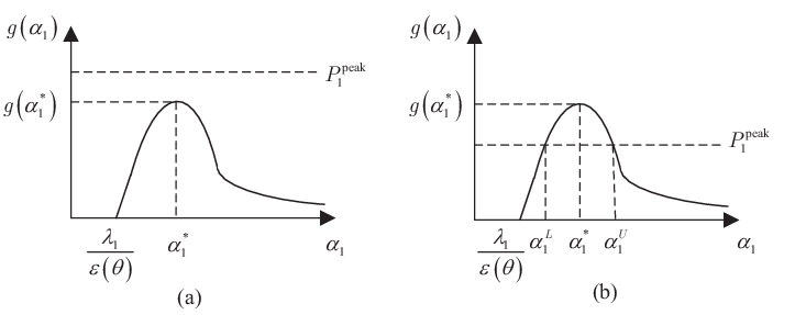
By solving (108), we can obtain the solution . It can be easily verified that the function first increases in the region of and then decreases when . Hence, we can obtain the maximum value of the function by substituting into (107), which yields
| (109) |
It can be readily verified that when , . In addition, . Hence, depending on the comparative value between and , two cases should be considered, when computing the average power as illustrated in Fig. 14. The details are given as follows:
Case I: . In this case, the transmit power is always lower than the peak power as shown in Fig. 14. Hence, the peak power constraints are redundant and can be removed. Thus, the average power can be expressed as
which can be expanded as (F), where is the exponential integral function, while is the upper incomplete gamma function.
Case II: . In this case, there must exist two solutions that satisfy as shown in Fig. 14. Denote these two solutions as and with . These two solutions can be numerically obtained by existing algorithms, such as the classic bisection search method. As seen from Fig. 14, the transmit power is equal to when and , equal to when . Hence, the average power can be expressed as:
| (113) |
Note that and can be derived similarly as the average power in Case I, which are omitted for simplicity. We only provide the expression of as follows:
where is the lower incomplete gamma function.
For the case of a single RRH, there is only one dual variable , which can be obtained by solving equation with one-dimension bisection search method.
Appendix G Proof of Lemma 3
For , the second-order derivative of with respect to (w.r.t.) is given by , which is positive since . Hence, is a convex function, when . Combining with the fact that , there are only three possible curves for when , as shown in Fig. 3. Next, we derive the conditions for each case.
- 1.
Case 1: In this case, the first-order derivative of is positive when , i.e., , which yields the condition for Case 1 in Lemma 3;
- 2.
Case 2: The first-order derivative of is negative for , i.e., , which yields the condition of . The minimum point of is achieved by solving equation , and the solution is given by . Then, according to Fig. 3-b, should hold, which leads to the second part of the conditions in Case 2 in Lemma 3;
- 3.
Case 3: The proof is similar to that in Case 2, and is omitted for simplicity.
Appendix H Proof of
It is easy to verify that when are given in (29). Hence, when the third condition of Lemma 3 given in Condition C1 is satisfied, according to Fig. 3-c, must fall into two regions: 1) ; 2) . In the following, we prove that the probability of falling into the second region is zero by using the method of contradiction.
Suppose that holds. Then, according to Fig. 3-c, must be larger than the optimal point, i.e., , where is given in Appendix G. By substituting in (29) into this inequality and after some further simplifications, we have
| (114) |
Additionally, by inserting in (29) into Condition C1 and after some further simplifications, we have
| (115) |
By substituting (115) into the right hand side of (114) and with some simple further operations, one obtains , which contradicts with (115) that . Hence, the assumption that cannot hold, which completes the proof.
Appendix I Derivations of when is a positive integer
The closed-form expression of for the case of can be easily obtained by inserting into (39). In the following, we only focus on the case when .
When , function can be expanded as [8.352.1, Page 899, [33]]
| (116) |
By plugging the above expression with into (39), we obtain the average power for RRH 1 as follows:
With some simple variable substitutions, the closed-form expressions of and can be easily calculated as in (43) and (44), respectively.
References
- [1] J. G. Andrews, S. Buzzi, W. Choi, S. V. Hanly, A. Lozano, A. C. K. Soong, and J. C. Zhang, “What will 5G be?” IEEE J. Sel. Areas Commun., vol. 32, no. 6, pp. 1065–1082, 2014.
- [2] M. Peng, S. Yan, and H. V. Poor, “Ergodic capacity analysis of remote radio head associations in cloud radio access networks,” IEEE Wireless Commun. Lett., vol. 3, no. 4, pp. 365–368, 2014.
- [3] Y. Shi, J. Zhang, and K. B. Letaief, “Group sparse beamforming for green cloud-RAN,” IEEE Trans. Wireless Commun., vol. 13, no. 5, pp. 2809–2823, 2014.
- [4] B. Dai and W. Yu, “Energy efficiency of downlink transmission strategies for cloud radio access networks,” IEEE J. Sel. Areas Commun., vol. 34, no. 4, pp. 1037–1050, 2016.
- [5] C. Pan, H. Zhu, N. J. Gomes, and J. Wang, “Joint precoding and RRH selection for user-centric green MIMO C-RAN,” IEEE Trans. Wireless Commun., vol. 16, no. 5, pp. 2891–2906, 2017.
- [6] D. Wu and R. Negi, “Effective capacity: a wireless link model for support of quality of service,” IEEE Trans. Wireless Commun., vol. 2, no. 4, pp. 630–643, 2003.
- [7] J. Tang and X. Zhang, “Quality-of-service driven power and rate adaptation over wireless links,” IEEE Trans. Wireless Commun., vol. 6, no. 8, pp. 3058–3068, 2007.
- [8] L. Musavian and S. Aissa, “Effective capacity of delay-constrained cognitive radio in Nakagami fading channels,” IEEE Trans. Wireless Commun., vol. 9, no. 3, pp. 1054–1062, 2010.
- [9] X. Zhang and J. Tang, “Power-delay tradeoff over wireless networks,” IEEE Trans. Commun., vol. 61, no. 9, pp. 3673–3684, 2013.
- [10] Y. Li, L. Liu, H. Li, J. Zhang, and Y. Yi, “Resource allocation for delay-sensitive traffic over LTE-advanced relay networks,” IEEE Trans. Wireless Commun., vol. 14, no. 8, pp. 4291–4303, 2015.
- [11] W. Cheng, X. Zhang, and H. Zhang, “Statistical-QoS driven energy-efficiency optimization over green 5G mobile wireless networks,” IEEE J. Sel. Areas Commun., vol. 34, no. 12, pp. 3092–3107, 2016.
- [12] C. E. Shannon, “A mathematical theory of communication,” ACM SIGMOBILE Mobile Computing and Communications Review, vol. 5, no. 1, pp. 3–55, 2001.
- [13] J. G. Smith, “The information capacity of amplitude-and variance-constrained sclar gaussian channels,” Information and Control, vol. 18, no. 3, pp. 203–219, 1971.
- [14] S. Shamai and I. Bar-David, “The capacity of average and peak-power-limited quadrature gaussian channels,” IEEE Transactions on Information Theory, vol. 41, no. 4, pp. 1060–1071, Jul 1995.
- [15] M. A. Khojastepour and B. Aazhang, “The capacity of average and peak power constrained fading channels with channel side information,” in 2004 IEEE Wireless Communications and Networking Conference (IEEE Cat. No.04TH8733), vol. 1, March 2004, pp. 77–82.
- [16] Q. Y. Yu, Y. T. Li, W. Xiang, W. X. Meng, and W. Y. Tang, “Power allocation for distributed antenna systems in frequency-selective fading channels,” IEEE Trans. Commun., vol. 64, no. 1, pp. 212–222, 2016.
- [17] M. K. Simon and M.-S. Alouini, Digital communication over fading channels. John Wiley & Sons, 2005, vol. 95.
- [18] G. Zhang, T. Q. S. Quek, A. Huang, M. Kountouris, and H. Shan, “Delay modeling for heterogeneous backhaul technologies,” in 2015 IEEE 82nd Vehicular Technology Conference (VTC2015-Fall), Sept 2015, pp. 1–6.
- [19] X. Chen, X. Xu, X. Tao, and H. Tian, “Dual decomposition based power allocation for downlink ofdm non-coherent cooperative transmission system,” in 2012 IEEE 75th Vehicular Technology Conference (VTC Spring), May 2012, pp. 1–5.
- [20] X. Chen, X. Xu, J. Li, X. Tao, T. Svensson, and H. Tian, “Optimal and efficient power allocation for ofdm non-coherent cooperative transmission,” in 2012 IEEE Wireless Communications and Networking Conference (WCNC), April 2012, pp. 1584–1589.
- [21] T. V. Chien, E. Bj?rnson, and E. G. Larsson, “Joint power allocation and user association optimization for massive mimo systems,” IEEE Transactions on Wireless Communications, vol. 15, no. 9, pp. 6384–6399, Sept 2016.
- [22] L. Liu, S. Bi, and R. Zhang, “Joint power control and fronthaul rate allocation for throughput maximization in ofdma-based cloud radio access network,” IEEE Transactions on Communications, vol. 63, no. 11, pp. 4097–4110, Nov 2015.
- [23] C. He, B. Sheng, P. Zhu, X. You, and G. Y. Li, “Energy- and spectral-efficiency tradeoff for distributed antenna systems with proportional fairness,” IEEE J. Sel. Areas Commun., vol. 31, no. 5, pp. 894–902, May 2013.
- [24] R. Zhang, “On peak versus average interference power constraints for protecting primary users in cognitive radio networks,” IEEE Trans. Wireless Commun., vol. 8, no. 4, pp. 2112–2120, 2009.
- [25] W. Yu and R. Lui, “Dual methods for nonconvex spectrum optimization of multicarrier systems,” IEEE Trans. Commun., vol. 54, no. 7, pp. 1310–1322, 2006.
- [26] S. Boyd and L. Vandenberghe, Convex optimization. Cambridge university press, 2004.
- [27] A. J. Goldsmith and P. P. Varaiya, “Capacity of fading channels with channel side information,” IEEE Transactions on Information Theory, vol. 43, no. 6, pp. 1986–1992, Nov 1997.
- [28] R. G. Stephen and R. Zhang, “Joint millimeter-wave fronthaul and ofdma resource allocation in ultra-dense cran,” IEEE Transactions on Communications, vol. 65, no. 3, pp. 1411–1423, March 2017.
- [29] Y. Li, M. Sheng, Y. Zhang, X. Wang, and J. Wen, “Energy-efficient antenna selection and power allocation in downlink distributed antenna systems: A stochastic optimization approach,” in 2014 IEEE International Conference on Communications (ICC), June 2014, pp. 4963–4968.
- [30] A. Helmy, L. Musavian, and T. Le-Ngoc, “Energy-efficient power adaptation over a frequency-selective fading channel with delay and power constraints,” IEEE Trans. Wireless Commun., vol. 12, no. 9, pp. 4529–4541, 2013.
- [31] E. U. T. R. Access, “Further advancements for E-UTRA physical layer aspects,” 3GPP TR 36.814, Tech. Rep., 2010.
- [32] C. She, C. Yang, and T. Q. S. Quek, “Cross-layer optimization for ultra-reliable and low-latency radio access networks,” IEEE Transactions on Wireless Communications, vol. 17, no. 1, pp. 127–141, Jan 2018.
- [33] I. S. Gradshteyn and I. M. Ryzhik, Table of integrals, series, and products. Academic press, 2014.