On Multi-source Networks: Enumeration, Rate Region Computation, and Hierarchy

Determining the capacity regions of networks under network coding form a highly important class of problems according to perspectives both theoretical and applied. Indeed, these problems are of fundamental importance in multi-terminal information theory, not only because the are the simplest – with independent sources, perfect channels, and lossless reconstruction – variants of general multiterminal problems, but also because solving all of these problems is equivalent to determining all of the fundamental laws of information theory [4, 5, 6, 7]. From a more practical viewpoint, optimized designs for many important modern engineering problems, including efficient information transfer over networks [8, 9], the design of efficient distributed information storage systems [10, 11], and the design of streaming media systems [12, 13, 14], have been shown to involve determining the rate region of an abstracted network under network coding. Yan et al.’s celebrated paper [15] has provided an exact representation of these rate regions of networks under network coding. Their essential result is that the rate region of a network can be expressed as the intersection of the region of entropic vectors [16, 17] with a series of linear (in)equality constraints created by the network’s topology and the sink-source requirements, followed by a projection of the result onto the entropies of the sources and edge variables. However, this is only an implicit description of the rate region, because the region of entropic vectors $\bar{\Gamma}_{N}^{*}$ is still unknown for $N\geq 4$.

Nevertheless, recent algorithmic developments have exploited this implicit characterization to enable computers to automatically determine and prove the capacity regions of small hypergraph networks under network coding [18, 19, 20, 21, 22]. Thanks to these algorithms and their implementations in packages like the information theoretic converse prover (ITCP) [23] and the the information theoretic achievability prover (ITAP) [24], it is now possible to very rapidly calculate the rate region, its proof, and the class of capacity achieving codes, for small networks, each of which would previously have taken a trained information theorist hours or longer to derive. The availability of these methods does not diminish the role of traditional theory proved by hand, rather, it shifts the questions driving theory development in new directions.

This article sets about developing a structural theory organizing and relating network coding problems of different sizes, whose aim is to make most efficient use of this newfound computational capability to determine capacity regions and their properties of networks of arbitrary size and scale. This structural theory consists of three components: minimality, symmetry, and hierarchy. In §III, a formal notion of network coding problem minimality is presented, which precisely describes how to remove from a network coding problem components which are redundant or irrelevant. For each such reduction, a theorem shows how the larger, non-minimal network, has a capacity region which can be directly inferred from the smaller one. The next component of the theory, symmetry, discussed in §IV, observes that in order to precisely formulate a network coding problem, labels must be applied to sources and edges, however the underlying problem is completely insensitive to the selection of these labels. Properly formulating the associated symmetry group through the language of group actions, together with a concise problem description aided by the notion of a minimal network, enable an algorithm for directly listing only the canonical and minimal representative of each large class of equivalent networks to be derived. This listing algorithm is used, together with the automated rate region calculation algorithms, in §V to generate a massive database containing the capacity regions of all hypergraph networks with the sum of sources and edges less than or equal to five. It is shown that for these small problems, linear codes suffice to exhaust the rate region and the Shannon outer bound is tight.

Finally, a hierarchical theory capable of inferring rate regions and properties from larger networks from smaller ones contained within them is presented. First, §VI, embedding operations, which recognize a small network coding problem embedded in a larger one, are defined and utilized, together with key theorems tracking rate regions through embeddings, to create the notion of forbidden network minors. These enable properties such as lack of sufficiency of a class of linear codes, or lack of tightness of the Shannon outer bound, to be determined for arbitrarily large networks by testing for inclusion of certain small problems within them. Next, desiring to construct the efficient codes of rate regions for large network coding problems by viewing them as being constructed from those of smaller networks, in §VII a series of combination operators are presented. §VIII then shows that together, the combinations and embedding operators enable solutions for large networks to be constructed through simple operations using rate regions of small networks as building blocks. The power of this hierarchy is demonstrated both by organizing the database, and showing how it, coupled with the database, can determine the capacity regions and their properties for massive numbers of networks of arbitrary scale.

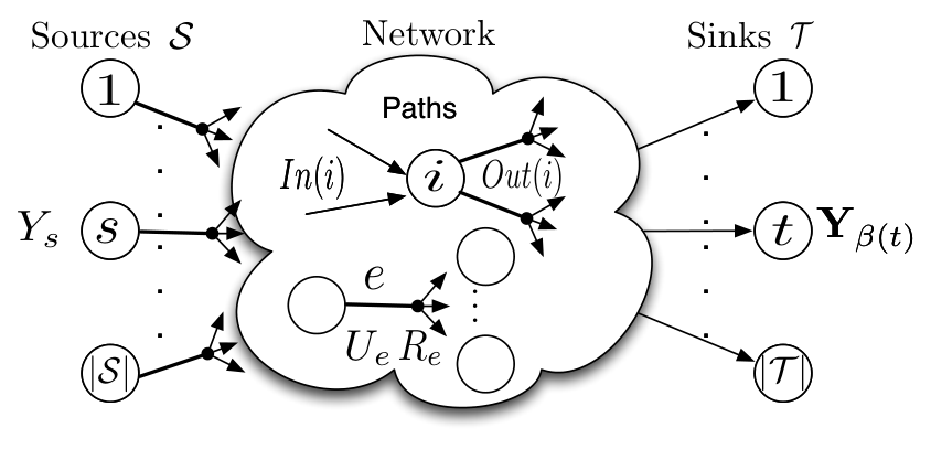
The class of problems under study in this paper are the rate regions of multi-source multi-sink network coding problems with hyperedges, which we hereafter refer to as the hyperedge MSNC problems. A network coding problem in this class, denoted by the symbol $\mathsf{A}$, includes a directed acyclic hypergraph $(\mathcal{V},\mathcal{E})$ [25] as in Fig. 1, consisting of a set of nodes $\mathcal{V}$ and a set $\mathcal{E}$ of directed hyperedges in the form of ordered pairs $e=(v,\mathcal{A})$ with $v\in\mathcal{V}$ and $\mathcal{A}\subseteq\mathcal{V}\setminus v$. The nodes $\mathcal{V}$ in the graph are partitioned into the set of source nodes $\mathcal{S}$, intermediate nodes $\mathcal{G}$, and sink nodes $\mathcal{T}$, i.e., $\mathcal{V}=\mathcal{S}\cup\mathcal{G}\cup\mathcal{T}$. Each of the source nodes $s\in\mathcal{S}$ will have a single outgoing edge $(s,\mathcal{A})\in\mathcal{E}$. The source nodes in $\mathcal{S}$ have no incoming edges, the sink nodes $\mathcal{T}$ have no outgoing edges, and the intermediate nodes $\mathcal{G}$ have both incoming and outgoing edges.

The number of sources will be denoted by $|\mathcal{S}|=K$, and each source node $s\in\mathcal{S}$ will be associated with an independent random variable $Y_{s}$, $s\in\mathcal{S}$, with entropy $H(Y_{s})$, and an associated independent and identically distributed (IID) temporal sequence of random values. For every source $s\in\mathcal{S}$, define ${\rm Out}(s)$ to be its single outgoing edge, which is connected to a subset of intermediate nodes and sink nodes. An edge $e\in\mathcal{E}$ connects a source, or an intermediate node to a subset of non-source nodes, i.e., $e=(i,\mathcal{F})$, where $i\in\mathcal{S}\cup\mathcal{G}$ and $\mathcal{F}\subseteq(\mathcal{G}\cup\mathcal{T}\setminus i)$. For an intermediate node $g\in\mathcal{G}$, we denote its incoming edges as ${\rm In}(g)$ and outgoing edges as ${\rm Out}(g)$.

For each edge $e=(i,\mathcal{F})$, the associated random variable $U_{e}=f_{e}({\rm In}(i))$ is a function of all the inputs of node $i$, obeying the edge capacity constraint $R_{e}\geq H(U_{e})$. The tail (head) node of edge $e$ is denoted as $\text{Tl}(e)$ ($\text{Hd}(e)$). For notational simplicity, the unique outgoing edge of each source node will be the source random variable, $U_{e}=Y_{s}$ if $\text{Tl}(e)=s$, denoting $\mathcal{E}_{S}=\{e\in\mathcal{E}|\text{Tl}(e)=s,s\in\mathcal{S}\}$ to be the variables associated with outgoing edges of sources, and $\mathcal{E}_{U}=\mathcal{E}\setminus\mathcal{E}_{S}$ to be the non-source edge random variables.

For each sink $t\in\mathcal{T}$, the collection of sources this sink will demand will be labeled by the non-empty set $\beta(t)\subseteq\mathcal{S}$. Collecting these definitions, a network can be represented as a tuple $\mathsf{A}=(\mathcal{S},\mathcal{G},\mathcal{T},\mathcal{E},\beta)$, where $\beta=(\beta(t),t\in\mathcal{T})$. For convenience, networks with $K$ sources and $L=|\mathcal{E}_{U}|$ edges are referred as $(K,L)$ instances.

As our focus in the manuscript will be on rate regions of a very similar form to those in [17, 15], this network coding problem model is as close to the original one in [17, 15] as possible while concisely covering the multiple instances of applications in network coding in which the same message can be overheard by multiple parties. These applications include index coding, wireless network coding, independent distributed source coding, and distributed storage, which are all covered concisely with this model as detailed in [26, 27].

It is in principle possible to transform the constraint of the same message being overheard by multiple parties into a directed acyclic graph used in [17, 15] by replacing each hyperedge $e=(i,\mathcal{F})$ in our model with a new vertex $v^{\prime}$ and $|\mathcal{F}|+1$ edges, $\{(i,v^{\prime})\}\cup\{(v^{\prime},j)|j\in\mathcal{F}\}$. However, this transformation effectively creates a far more difficult and complicated rate region, as each of the $|\mathcal{F}|$ new edges $\{(v^{\prime},j)|j\in\mathcal{F}\}$ must also have associated new random variables and new rate constraints in the model of [17, 15]. As the complexity of determining the rate region through the implicit characterization in [17, 15] is at least exponentially dependent on the number of random variables, such a transformation of a problem with, in truth, a concise hypergraph structure, into a larger more complicated ordinary directed graph one is ill-advised. It is for this reason we depart notationally from the commonly used model from [17, 15]. Aside from this minor difference, the notion of a network code, an achievable rate vector, and the capacity region can be defined [26, 27] in an analogous manner to [17, 15].

Defining $\mathcal{L}_{i},i=1,3,4^{\prime},5$ as network constraints representing source independence, coding by intermediate nodes, edge capacity constraints, and sink nodes decoding constraints respectively,

and denoting $\mathcal{L}_{13}=\mathcal{L}_{1}\cap\mathcal{L}_{3}$, $\mathcal{L}_{4^{\prime}5}=\mathcal{L}_{4^{\prime}}\cap\mathcal{L}_{5}$ and $\mathcal{L}_{\mathsf{A}}=\mathcal{L}_{1}\cap\mathcal{L}_{3}\cap\mathcal{L}_{4^{\prime}}\cap\mathcal{L}_{5}$, the implicit characterization from [17, 15] is translated in [26, 27] to the following one.

While the analytical expression determines, in principle, the rate region of any network under network coding, it is only an implicit characterization. This is because $\Gamma_{N}^{*}$ is unknown and even non-polyhedral for $N\geq 4$. Further, while $\bar{\Gamma}^{*}_{N}$ is a convex cone for all $N$, $\Gamma^{*}_{N}$ is already non-convex by $N=3$, though it is also known that the closure only adds points at the boundary of $\bar{\Gamma}^{*}_{N}$. Thus, the direct calculation of rate regions from (1) for a network with 4 or more variables is infeasible. On a related note, at the time of writing, it appears to be unknown by the community whether or not the closure after the conic hull is actually necessary¹¹ 1 The closure would be unnecessary if $\bar{\Gamma}^{*}_{N}=\textrm{con}(\Gamma^{*}_{N})$, i.e. if every extreme ray in $\bar{\Gamma}^{*}_{N}$ had at least one point along it that was entropic (i.e. in $\Gamma^{*}_{N}$). At present, all that is known is that $\Gamma^{*}_{N}$ has a solid core, i.e. that the closure only adds points on the boundary of $\bar{\Gamma}^{*}_{N}$. in (1), and the uncertainty that necessitates its inclusion muddles a number of otherwise simple proofs and ideas. For this reason, some of the discussion in the remainder of the manuscript will study a closely related inner bound $\mathcal{R}_{*}(\mathsf{A})$ to $\mathcal{R}_{c}(\mathsf{A})$ described in the following corollary, which also introduces polyhedral inner and outer bounds through it. In all of the cases where the rate region has been computed to date $\mathcal{R}_{c}(\mathsf{A})=\mathcal{R}_{*}(\mathsf{A})$.

Of particular interest in this manuscript are the rate region bounds $\mathcal{R}_{o}(\mathsf{A}),\mathcal{R}_{s,q}(\mathsf{A}),\mathcal{R}_{q}^{N^{\prime}}(\mathsf{A}),\mathcal{R}_{q}(\mathsf{A}),\mathcal{R}_{{\rm linear}}(\mathsf{A})$ built from the Shannon outer bound $\Gamma_{N}$ [28, 29], scalar linear codes over the finite field $\mathbb{F}_{q}$, vector linear codes over $\mathbb{F}_{q}$ of total dimension at most $N^{\prime}$, all vector linear codes over $\mathbb{F}_{q}$, and timesharing vector linear codes over possibly different finite fields, respectively [26, 27].

As is clear from their definition $\mathcal{R}_{s,q}(\mathsf{A})\subseteq\mathcal{R}_{q}^{N^{\prime}}(\mathsf{A})\subseteq\mathcal{R}_{q}(\mathsf{A})\subseteq\mathcal{R}_{{\rm linear}}(\mathsf{A})\subseteq\mathcal{R}_{o}(\mathsf{A})$.

Thanks to [30], $\Gamma_{N}^{{\rm linear}}$ is known for $N\leq 5$, but for $N\geq 6$, [30, 31] show that there are new inequalities for each $N-1$ to $N$, and $\Gamma_{N}^{{\rm linear}}$ remains unknown. Hence, a calculation of $\mathcal{R}_{{\rm linear}}(\mathsf{A})$ via the projection process in (9) is only feasible for $N\leq 5$.

The information theoretic converse prover [23, 18] can calculate $\mathcal{R}_{o}(\mathsf{A})$ for larger, yet still small, numbers of variables $N\leq 8$, while the information theoretic achievability prover [24, 19] can calculate $\mathcal{R}_{q}^{N^{\prime}}(\mathsf{A})$ for small field sizes and even larger $N^{\prime}$. As is described in the articles [18] and [19], respectively, these two pieces of software use sophisticated methods, beyond naïve calculation of the bound to $\Gamma_{N}^{*}$ followed by polyhedral projection as is verbatim suggested by (5), to push the number of variables $N$ to be as large as possible. However, these methods are still overall limited to somewhat small problems.

The remainder of this manuscript develops a structural theory that enables these tools to determine the capacity region and its bounds for problems beyond the scale they can directly reach. The first order of business, undertaken in the next section, is to identify and remove components of the network coding problem description $\mathsf{A}$ inessential to the core problem complexity. Subsequent sections will then set about constructing network generation tools required to build a massive database of solved network coding rate regions, organizing this database through embedding operators, and extending it to larger networks via both embedding and combinations operators.

Though in principle, any network coding problem as described in §II forms a valid network coding problem, such a problem can include networks with nodes, edges, and sources which are completely extraneous and unnecessary from the standpoint of determining the rate region. To deal with this, in this section, we show how to form a network instance with equal or fewer number of sources, edges, or nodes, from an instance with extraneous components. We will show the rate region of the instance with the extraneous components can be directly inferred from the rate region of the reduced network. Network coding problems without such extraneous and unnecessary components will be called minimal.

The intuition supporting each of the 14 minimality conditions is provided in Fig. 2. The key idea behind minimality is that if a network is non-minimal, we can replace it with a minimal one, determine the rate region of the minimal network, then perform simple operations on the rate of the minimal network to get the rate region of the non-minimal one. These operations are captured in Table II.

Even though the notion of network minimality (§III) reduces the set of network coding problem instances by removing parts of a network coding problem which are inessential, much more needs to be done to group network coding problem instances into appropriate equivalence classes. An important notion of equivalent problems arises from symmetries between different problems. Symmetries between different network coding problems arise because although we have to use label sets to describe the edges and sources in order to specify a network coding problem instance (identifying a certain source as source number one, another as source number two, and so on), it is clear that the essence of the underlying network coding problem is insensitive to these labels. Two networks differing only in the selection of these labels are clearly equivalent. Our goal in this section is to first formalize this notion of equivalence through relabeling, then devise an algorithm which can directly list one network coding problem representative from each equivalence class.

References

- [1] C. Li, S. Weber, and J. Walsh, “Network embedding operations preserving the insufficiency of linear network codes,” in 52nd Annual Allerton Conference on Communication, Control, and Computing (Allerton), 2014, Oct 2014.
- [2] C. Li, S. Weber, and J. M. Walsh, “Computer aided proof for rate regions of independent distributed source coding problems,” in IEEE International Symposium on Network Coding (NetCod), Jun 2015.
- [3] C. Li, S. Weber, and J. Walsh, “Network combination operations preserving the sufficiency of linear network codes,” in IEEE Information Theory Workshop (ITW), 2015, submitted.
- [4] T. Chan and A. Grant, “Dualities between entropy functions and network codes,” IEEE Transactions on Information Theory, vol. 54, no. 10, pp. 4470–4487, October 2008.
- [5] T. Chan and A. Grant, “Entropy Vectors and Network Codes,” in IEEE International Symposium on Information Theory, Jun. 2007.
- [6] T. Chan and A. Grant, “Dualities between entropy functions and network codes,” in Fourth Workshop on Network Coding, Theory and Applications (NetCod), January 2008.
- [7] ——, “Mission impossible: computing the network coding capacity region,” in IEEE International Symposium on Information Theory (ISIT), July 2008, pp. 320–324.
- [8] R. Ahlswede, N. Cai, S.-Y. Li, and R. Yeung, “Network information flow,” IEEE Transactions on Information Theory, vol. 46, no. 4, pp. 1204–1216, Jul 2000.
- [9] R. Dougherty, C. Freiling, and K. Zeger, “Networks, matroids, and non-shannon information inequalities,” IEEE Transactions on Information Theory, vol. 53, no. 6, pp. 1949–1969, 2007.
- [10] A. Dimakis, P. Godfrey, Y. Wu, M. Wainwright, and K. Ramchandran, “Network coding for distributed storage systems,” IEEE Transactions on Information Theory, vol. 56, no. 9, pp. 4539–4551, Sept 2010.
- [11] C. Tian, “Characterizing the rate region of the (4,3,3) exact-repair regenerating codes,” IEEE Journal on Selected Areas in Communications, vol. 32, no. 5, pp. 967–975, May 2014.
- [12] J. Walsh, S. Weber, and C. Maina, “Optimal rate–delay tradeoffs and delay mitigating codes for multipath routed and network coded networks,” Information Theory, IEEE Transactions on, vol. 55, no. 12, pp. 5491–5510, Dec 2009.
- [13] S. Weber, C. Li, and J. M. Walsh, “Rate region for a class of delay mitigating codes and p2p networks,” 46th Annual Conference on Information Sciences and Systems, March 2012.
- [14] D. Leong, A. Qureshi, and T. Ho, “On coding for real-time streaming under packet erasures,” in Information Theory Proceedings (ISIT), 2013 IEEE International Symposium on, July 2013, pp. 1012–1016.
- [15] X. Yan, R. Yeung, and Z. Zhang, “An implicit characterization of the achievable rate region for acyclic multisource multisink network coding,” IEEE Transactions on Information Theory, vol. 58, no. 9, pp. 5625–5639, Sept 2012.
- [16] Z. Zhang and R. Yeung, “On characterization of entropy function via information inequalities,” Information Theory, IEEE Transactions on, vol. 44, no. 4, pp. 1440–1452, Jul 1998.
- [17] R. W. Yeung, Information Theory and Network Coding. New York, US: Springer, 2008.
- [18] Jayant Apte and John MacLaren Walsh, “Explicit Polyhedral Bounds on Network Coding Rate Regions via Entropy Function Region: Algorithms, Symmetry, and Computation,” IEEE Trans. Inf. Theory, 2016, Submitted July 22, 2016. [Online]. Available: http://arxiv.org/abs/1607.06833
- [19] ——, “Constrained Linear Representability of Polymatroids and Algorithms for Computing Achievability Proofs in Network Coding,” IEEE Trans. Inf. Theory, Submitted May 15, 2016. [Online]. Available: http://arxiv.org/abs/1605.04598
- [20] C. Li, S. Weber, and J. M. Walsh, “Multilevel diversity coding systems: Rate regions, codes, computation, forbidden minors,” IEEE Transactions on Information Theory, vol. 63, no. 1, pp. 230–251, 2017.
- [21] C. Li, J. Apte, J. M. Walsh, and S. Weber, “A new computational approach for determining rate regions and optimal codes for coded networks,” in IEEE International Symposium on Network Coding (NetCod), Jun 2013, pp. 1 –6.
- [22] C. Li, J. M. Walsh, and S. Weber, “Computational approaches for determining rate regions and codes using entropic vector bounds,” in 50th Annual Allerton Conference on Communication, Control and Computing, Oct 2012, pp. 1 –9.
- [23] Jayant Apte and John MacLaren Walsh, “Information Theoretic Converse Prover.” [Online]. Available: https://github.com/jayant91089/itcp
- [24] ——, “Information Theoretic Achievability Prover.” [Online]. Available: https://github.com/jayant91089/itap
- [25] G. Gallo, G. Longo, S. Pallottino, and S. Nguyen, “Directed hypergraphs and applications,” Discrete applied mathematics, vol. 42, no. 2, pp. 177–201, 1993.
- [26] Congduan Li, “On Multi-source Multi-Sink Hyperedge Networks: Enumeration, Rate Region Computation, and Hierarchy,” Ph.D. dissertation, Drexel University, Philadelphia, PA, 2015. [Online]. Available: http://www.ece.drexel.edu/walsh/CongduanLi_PhD.pdf
- [27] C. Li, S. Weber, and J. M. Walsh, “On multi-source networks: Enumeration, rate region computation, and hierarchy,” CoRR, vol. abs/1507.05728, 2015. [Online]. Available: http://arxiv.org/abs/1507.05728
- [28] Raymond W. Yeung, “A Framework for Linear Information Inequalities,” IEEE Trans. on Information Theory, vol. 43, no. 6, Nov. 1997.
- [29] Zhen Zhang and Raymond W. Yeung, “On Characterization of Entropy Function via Information Inequalities,” IEEE Trans. on Information Theory, vol. 44, no. 4, Jul. 1998.
- [30] R. Dougherty, C. Freiling, and K. Zeger, “Linear rank inequalities on five or more variables,” arXiv cs.IT/0910.0284v3, 2009.
- [31] R. Kinser, “New inequalities for subspace arrangements,” Journal of Combinatorial Theory Series A, vol. 118, no. 1, pp. 152–161, January 2011.
- [32] J. Apte and J. Walsh, “Symmetry in network coding,” in 2015 IEEE International Symposium on Information Theory (ISIT), June 2015.
- [33] J. Apte and J. M. Walsh, “Exploiting symmetry in computing polyhedral bounds on network coding rate regions,” in IEEE International Symposium on Network Coding (NetCod), Jun 2015.
- [34] A. Betten, M. Braun, H. Fripertinger, A. Kerber, A. Kohnert, and A. Wassermann, Error-Correcting Linear Codes: Classification by Isometry and Applications, ser. Algorithms and Computation in Mathematics. Springer Berlin Heidelberg, 2006.
- [35] B. Schmalz, “-Designs zu vorgegebener Automorphismengruppe,” Bayreuther Mathematische Schriften, no. 41, pp. 1–164, 1992, Dissertation, Universität Bayreuth, Bayreuth.
- [36] GAP – Groups, Algorithms, and Programming, Version 4.7.7, The GAP Group, 2015. [Online]. Available: http://www.gap-system.org
- [37] T. Rehn and A. Schürmann, “C++ tools for exploiting polyhedral symmetries,” Lecture Notes in Computer Science, vol. 6327/2010, 2010.
- [38] John MacLaren Walsh and Congduan Li, “Network Enumeration and Hierarchy in GAP.” [Online]. Available: http://www.ece.drexel.edu/walsh/aspitrg/software.html
- [39] C. Li, J. M. Walsh, and S. Weber, “TransIT 2015 Data: Enumeration and Rate Regions for General Hyperedge Networks,” available at https://goo.gl/lyZfD9.
- [40] R. W. Yeung and Y. O. Yan, “Information theoretic inequality prover,” 2008, http://user-www.ie.cuhk.edu.hk/ ITIP/.
- [41] E. Rethnakaran Pulikkoonattu and Suhas Diggavi, “X-information theoretic inequality prover,” 2008, http://user-www.ie.cuhk.edu.hk/ ITIP/.
- [42] L. Csirmaz, “a MINimal Information Theoretic Inequality Prover,” https://github.com/lcsirmaz/minitip.
- [43] Zhen Zhang and Raymond W. Yeung, “A Non-Shannon-Type Conditional Inequality of Information Quantities,” IEEE Trans. on Information Theory, vol. 43, no. 6, Nov. 1997.
- [44] R. Dougherty, C. Freiling, and K. Zeger, “Networks, Matroids, and Non-Shannon Information Inequalities,” IEEE Trans. on Information Theory, vol. 53, no. 6, pp. 1949–1969, Jun. 2007.
- [45] H. Sun and S. A. Jafar, “Index coding capacity: How far can one go with only shannon inequalities?” IEEE Transactions on Information Theory, vol. 61, no. 6, pp. 3041–3055, June 2015.
- [46] A. S. N. V. D. Hammer, A. Romashchenko, “Inequalities for Shannon Entropy and Kolmogorov Complexity,” Journal of Computer and System Sciences, no. 60, pp. 442–464, 2000.
- [47] Randall Dougherty, Chris Freiling, Kenneth Zeger, “Linear rank inequalities on five or more variables,” submitted to SIAM J. Discrete Math. arXiv:0910.0284.
- [48] Randall Dougherty, Chris Freiling, and Ken Zeger, “Insufficiency of linear coding in network information flow,” IEEE Trans. Inf. Theory, vol. 51, no. 8, pp. 2745–2759, Jul. 2005.
- [49] A. W. Ingleton, “Representation of Matroids,” in Combinatorial Mathematics and its Applications, D. J. A. Welsh, Ed. San Diego: Academic Press, 1971, pp. 149–167.
- [50] T. Ho, M. Effros, and S. Jalali, “On equivalence between network topologies,” in 2010 48th Annual Allerton Conference on Communication, Control, and Computing (Allerton), Sept 2010, pp. 391–398.
- [51] X. Xu, S. Thakor, and Y. L. Guan, “Reduced functional dependence graphs and their applications,” in 2012 International Symposium on Network Coding (NetCod), June 2012, pp. 61–66.
- [52] N. Robertson and P. Seymour, “Graph minors. i. excluding a forest,” Journal of Combinatorial Theory, Series B, vol. 35, no. 1, pp. 39 – 61, 1983.
- [53] ——, “Graph minors. xx. wagner’s conjecture,” Journal of Combinatorial Theory, Series B, vol. 92, no. 2, pp. 325 – 357, 2004, special Issue Dedicated to Professor W.T. Tutte.
- [54] P. D. Seymour, “Matroid Representation over GF(3),” J. Combin. Theory Ser. B, no. 26, pp. 159–173, 1979.
- [55] James Oxley, Matroid Theory, 2nd. Ed. Oxford University Press, 2011.
- [56] J. Geelen, B. Gerards, and G. Whittle, “Solving rota’s conjecture,” Notices of the American Mathematical Society, pp. 736–743, 2014.
- [57] Congduan Li, Steven Weber, and John MacLaren Walsh, “On Multilevel Diversity Coding Systems,” IEEE Trans. Inf. Theory, vol. 63, no. 1, pp. 230–251, Jan. 2017. [Online]. Available: https://doi.org/10.1109/TIT.2016.2628791
- [58] C. Li, J. M. Walsh, and S. Weber, “Software for computing bounds on entropic vectors region and network rate region,” available at http://www.ece.drexel.edu/walsh/aspitrg/software.html.
- [59] ——, “ITW 2015 Data: Enumeration and Exact Rate Regions for Networks,” available at http://goo.gl/f1spQz.
- [60] ITAP – Information Theoretic Achievability Prover, Adaptive Signal Processing and Information Theory Research Group, 2015. [Online]. Available: http://www.ece.drexel.edu/walsh/aspitrg/software.html
- [61] ITCP – Information Theoretic Converse Prover, Adaptive Signal Processing and Information Theory Research Group, 2016. [Online]. Available: http://www.ece.drexel.edu/walsh/aspitrg/software.html
Appendix A Proof of Theorem 2
In the interest of conciseness, for all but (D4) and (D8) we will only briefly sketch the proof for the expressions determining from , as the map in the opposite direction and the other rate region bounds follow directly from parallel arguments.
(D1) holds because is not communicating with any nodes other than possibly sinks. If there is a sink that demands it that does not have direct access to it, then this sink can not successfully receive any information from it, since does not communicate with any intermediate nodes. Hence, in this case and every other rate is constrained according to because the remainder of the network has no interaction with . Alternatively, if every sink that demands has direct access to it, any non-negative source rate can be supported for , and the remainder of the network is constrained as by because no other part of the network interacts with .
(D2) holds because the demand of at sink is trivially satisfied if it has direct access to . The constraint has no impact on the rate region of the network.
In (D3) if a source is not demanded by anyone, it can trivially support any rate.
When two sources have exactly the same connections and are demanded by same sinks as under (D4), they can be simply viewed as a combined source for with , since the exact region and these bounds enable simple concatenation of sources. Since the source entropies are variables in the rate region expression, it is equivalent to make as the combined source, which since the previous sources were independent, will have an entropy which is the sum of their entropies. Moving from to is then accomplished for any by observing that can be viewed as with .
An intermediate node can only utilize its input hyperedges to produce its output hyperedges, hence when two intermediate nodes have the same input edges, their encoding capabilities are identical, and thus for pursuing minimality of representation of a network, these two nodes having the same input should be represented as one node. Thus, (D5) is necessary and the merge of nodes with same input does not impact the coding on edges or the rate region, as the associated constraints .
If the input or output of an intermediate node is empty, as in (D6) it is incapable of affecting the capacity region. If, as in the second case covered by (D6) the input to an sink node is empty, any sources which it demands can only be reliably decoded if they have zero entropy.
(D7) is clear because an edge to nowhere can not effect the rest of the capacity region and is effectively unconstrained itself.
(D8) can be shown as follows. If is known and when edge in is represented as two parallel edges so that the network becomes , then the constraint on in is simply to make sure the total capacity can allow the information to be transmitted from the tail node to head nodes. Simple concatenation of the messages among the two edges will achieve this for those bounds allowing such concatenation. Therefore, replace the in with will obtain the rate region for any . Moving from to is accomplished by recognizing that is effectively with .
Under the condition in (D9), an intermediate node has exactly one input edge and exactly one output hyperedge , and the input is an edge (i.e. is its only destination). The rate coming out of this node can be no larger than the rate coming in since the single output hyperedge must be a deterministic function of the input edge. It suffices to treat these two edges as one hyperedge connecting the tail of to the head of with the rate the minimum of the two rates.
If a sink demands a source that it does not have access to, the only way to satisfy this network constraint is the source entropy is . Hence, (D10) holds. The removal of this redundant source does not impact the rate region of the network with remaining variables.
(D11), similar to (D3), observes that two sink nodes with same input yield the same constraints as with them merged.
(D12) is easy to understand because the decoding ability of at sink node is implied by sink . The non-necessary repeated decoding constraints will not affect the rate region.
(D13), as (D12), observes that the ability of to decode implies that can decode it as well. Adding or removing the direct access to at will not affect the rate region.
(D14) is obviously true since the weakly disconnected components can not influence each others rate regions.
Appendix B Proof of Theorem 4
We will prove for , and for the scalar case, , since the remainder of the theorem holds from the minimality reductions in Thm. 2.
Select any point . Then there exists a conic combination of some points in that are associated with entropic vectors in such that , where . For each , there exist random variables , such that the entropy vector
is in , where is the number of variables in . Furthermore, their entropies satisfy all the constraints determined by . In the network , define to be the concatenation of all inputs to the tail node of , . Then the entropies of random variables will satisfy the constraints in , and additionally obey . Hence, . That is, . By using the same conic combination, we have an associated rate point . Thus, , which in turn, is .
If is achievable by general codes, since concatenation of all input is a valid vector code, we have which in turn is
However, we cannot establish same relationship when scalar codes are considered, because for the point , the associated with may not be scalar achievable.
On the other hand, if we select any point , then, there exists a conic combination of some points in associated with entropic vectors in , i.e., . For each , there exist random variables such that their entropies satisfy all the constraints determined by . Since the entropies of satisfy all constraints determined by (because they are a subset of the constraints from ) and the entropic vector projecting out is still entropic. Thus, by letting to be unconstrained, we have Further, by using the same conic combination, . Thus, we have .
If is achievable by code , either scalar or vector, then the code to achieve could be the code with deletion of columns associated with edge , i.e., , because the code on edge is not of interest. Thus, we have
Furthermore, for any point , there exists an associated point and a rate vector such that . Clearly, if we increase the dimension of by adding a variable which is the vector of all input variables to the tail node of , i.e., and , we have the new vector in . That is, if we define