Structure-Dynamics Relation in Physically-Plausible Multi-Chromophore Systems
Abstract
We study a large number of physically-plausible arrangements of chromophores, generated via a computational method involving stochastic real-space transformations of a naturally occurring ‘reference’ structure, illustrating our methodology using the well-studied Fenna-Matthews-Olson complex (FMO). To explore the idea that the natural structure has been tuned for efficient energy transport we use an atomic transition charge method to calculate the excitonic couplings of each generated structure and a Lindblad master equation to study the quantum transport of an exciton from a ‘source’ to a ‘drain’ chromophore. We find significant correlations between structure and transport efficiency: High-performing structures tend to be more compact and, among those, the best structures display a certain orientation of the chromophores, particularly the chromophore closest to the source-to-drain vector. We conclude that, subject to reasonable, physically-motivated constraints, the FMO complex is highly attuned to the purpose of energy transport, partly by exploiting these structural motifs.
The process of excitonic energy transport is of great interest across many fields of study, from evolutionary biology to the engineering of solar cells. It is a key component of both natural photosynthesis (occurring in light harvesting complexes (LHCs), which are assemblages of chromophores found in a famously ‘warm and wet’ environment) and artificial photovoltaics. It is tempting to suggest that, since natural selection has had perhaps billions of years [1] over which to improve the efficiency of the process, we might learn from nature how to better engineer artificial light harvesting systems. This view has gathered interest in recent years, in tandem with claims that naturally occurring systems can exhibit outstandingly high efficiency [2, 3]. It is often said that quantum coherence could play a pivotal role in enhancing transport [4, 5, 6, 7] through constructive interference of excitation pathways (although this is hotly debated [8, 9, 10]) and that the structural arrangement of chromophores has been optimised for this functionality [3]. Contrariwise, it might be suggested that efficient transport through a network of chromophores is actually generic and most of the possible structural arrangements would show similar performance. It is difficult to draw conclusions about the general structure-dynamics relationship from studying only a handful of naturally occurring LHCs. Indeed, while it is clearly desirable to learn from the results of natural selection [11], we must also be able to relax the constraints that it operated under in order to uncover the potential for technological advantage, while at all times keeping our imagination on a short enough leash so that any new structures remain physically plausible.
Theoretical efforts have so far proceeded along two paths. The first technique is to randomly ‘sprinkle’ point-like electrical dipoles into a restricted volume: This approach has allowed the use of genetic algorithms to optimise their positions [12], and later showed how fast transport is typically aided by a ‘backbone plus pair’ geometry by reinforcing constructive interference [13], and correlated to the centrosymmetry of the Hamiltonian describing the energy of the system [14]. The spatial density of dipoles was considered [15], and (although generally correlated with efficient exciton transport) was found to saturate to the densities typically found in natural LHCs [16]. A drawback of such approaches is that they may not have much to say about realistic systems, whose structure and properties are determined by more complicated, highly-constrained relations between anisotropic molecules extended in physical space.
The second technique begins with a commonly accepted mathematical model of an existing system, and performs perturbations on it. This approach has enabled investigations of robustness and identification of dominant transport pathways in a naturally occurring LHC [14], as well as transport efficiency in purple bacteria compared with counterfactual structures, obtained through rotating [10] or ‘trimming’ [18] chromophores from the LH1 and LH2 complexes. The latter works speculate on the relative importance of coherent supertransfer in these systems (noting that it is a ‘spandrel’ – or evolutionary byproduct – rather than an adaption) as well as the degree of attunedness of the original structure for energy transport. A possible drawback of these approaches, as we explain below, is the potential physical implausibility of the perturbed models, especially when the transformations involve ‘deleting’ coupling terms or making uncorrelated perturbations to the Hamiltonian matrix. Other strategies deploy abstract models of the transport system [19, 13, 21, 22, 23] to learn general principles from idealised ‘network’ models that may operate to a greater or lesser extent in realistic systems.
In this Letter, we incorporate the best of the above strategies to address two key questions on the structure-dynamics relationship for exciton transport: (i) which structural motifs influence exciton dynamics in typical physically-plausible multi-chromophore complexes? and (ii) do naturally occurring complexes appear to be attuned for certain transport tasks (by exploiting these motifs or otherwise)? We proceed by simulating the transport properties of a large number of artificial, or ersatz structures obtained from a reference one by geometrical perturbations (GPs).

We generate a sample of plausible structures, associating to each an Hamiltonian matrix representing a network of chromophores where a single excitation can exist. We take the naturally occurring Fenna-Matthews-Olson (FMO) complex [24] as our reference structure, chosen for its simplicity and relevance as a model system for LHCs [25] (although our methodology could however just as well be applied to any LHC). Present in species of green sulfur bacteria, the complex takes the form of three identical protein monomers, each of which comprising a protein matrix which contains identical bacteriochlorophyll-a (BChl) chromophores [26] (see Fig. 1). As we will be interested in exciton transport between BChls 1 (‘source’, closest to the antenna) and 3 (‘drain’, closest to the reaction centre), we fix their position, while the other 6 BChls are rigidly displaced and rotated by a sequence of Monte-Carlo moves, starting with their reference locations [4, 5, 6]. During the GP, we retain only plausible ersatz structures by rejecting those where the minimum inter-atomic separation between the BChls is smaller than a cut-off intermediate between bonding and van der Waals distances; and contain the geometric centroid of each BChl within a sphere of radius from the midpoint between BChls 1 and 3 (roughly representing the volume contained by the protein matrix in the reference structure).
To each ersatz structure we associate the excitonic Hamiltonian
| (1) |
This expression is written with respect to an orthonormal set of basis states , each representing the situation where BChl is excited and all other BChls are not. The first structure is our reference structure. The diagonals represent the energy landscape for non-interacting chromophores. While some previous studies set their distribution to be uniform [12], we retain a non trivial distribution by fixing the diagonals to those corresponding to the reference FMO (see supplementary information S4 and S6). An energy gradient, aided by a bath-mediated relaxation, can ‘funnel’ excitations towards lower-lying excited states. Although our modelling of the bath forbids this relaxation, we argue that these ‘site’ energies can be nevertheless very influential on the exciton dynamics. They determine the energy eigenstates of and therefore influence the phase relationship and subsequent interference between different pathways through the network. .
The off-diagonal elements arise from Coulomb interactions between transition charge densities, and depend on the mutual orientation of the chromophores. It is well known that a simple point-dipole approximation to would break down at the short distances we consider [30]: we therefore adopt a superior approach [31], partitioning the atomic transition density for each structure into atomic transition charges (with coordinates ) centred on atom of chromophore . The Coulombic interaction is then summed to evaluate the coupling
| (2) |
The matrix elements in Eqn. (2) are scaled by the factor to capture the dielectric effect of protein and solvent [10].
We use a phenomenological dynamical model for the motion of a single exciton through our network of chromophores. While several variations [33] and more elaborate models exist [34], our Lindblad master equation captures the essential effects of dephasing and dissipation, and represents a completely positive transformation [35] on the density matrix . Defining , we have
| (3) |
The first term represents closed-system dynamics, and the other terms represent effects arising from interaction with an environment, with the collapse operators taken to be independent of the structure index and given by
| (4) |
We have expanded the Hilbert space to include and (environment) which are states accessible through dissipation but which cannot build up any coherence with the rest of the network. Here, is a fast and irreversible process that represents successful capture of the exciton at BChl 3, where it is transferred to a reaction centre, or ‘sink’ [1]. All other incoherent processes operate independently of the chromophore index . represents the relatively slow process of exciton dissipation (or decay). The term represents the averaged coupling of BChl to its vibrational environment, leading to a local loss of coherence. If this happens too quickly, the exciton can be ‘frozen’ and prevented from evolving as per the Zeno effect [36]. If dephasing is too slow, destructive interference can lock the exciton in a particular subspace [13, 37]. We choose rates extracted from spectroscopy experiments at 77K [38], but our conclusions are robust to moderate changes in these values (see supplementary information S1).
Although the choice of a realistic initial condition for the exciton transport is the subject of some debate [39], we set an exciton localised on BChl 1 (our ‘source’). This is consistent with the accepted photo-excitation process, which occurs in the nearby chlorosome (which acts as an antenna [1]). We numerically solve the Lindblad master equation for , which can be thought of as a Hilbert-space operator ‘trajectory’ associated with each ersatz structure. It is this association which will allow us to explore the structure-dynamics relationship.
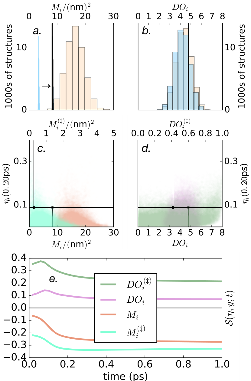
First we consider how compact the chromophores are along the ‘transport vector’ which connects the source and drain (see Fig. (1)). Define
| (5) |
(the mass-normalised moment of inertia), where is the perpendicular distance of each atom in structure to the transport vector and the sum is taken only over the coordinates of the Magnesium atoms that lie roughly in the centre of each BChl. Fig. (2a) shows that the vast majority of our sample has . We infer that it is difficult to pack the BChls into a volume smaller than nature has, without having unreasonably short distances between chromophores. We will return to this point later on.
Our focus is on investigating the structural properties of those randomly generated structures which perform ‘best’ at some exciton transport function, e.g. fast or high-yield transport; high-retention storage or even fast energy-dissipation. Those structures performing well can be inspected for characteristics which might form the basis of design principles for synthetic applications. Here, we quantify the performance of our dynamics via the transport efficiency
| (6) |
which measures both the speed and yield of energy transfer.
To identify the main structural motifs influencing the exciton dynamics we use the Spearman rank correlation coefficient . Ranging between and , the coefficient measures the extent to which two quantities and are monotonically related (see supplementary information S3). In this work, we fix and begin with Fig. (2c,e) shows an inverse correlation between the moment of inertia and the transport efficiency . Structures that are more compact tend to exhibit faster transport.
In fact, this realisation has a bearing on the second of our key questions (ii): To investigate the relative performance of the reference structure, we introduce the normalised rank (henceforth ‘rank’) defined as
| (7) |
where is the ordinal rank by measure through our sample of ersatz structures. Thus, at time , the reference structure has equal to one (zero) if it has the highest (lowest) among all ersatz structures in the sample. A rank of 0.5 means there are as many ersatz structures outperforming as underperforming the reference. The standard deviation of is written as , with . It has its usual statistical definition (as the square root of the variance), and gives an idea of the overall variation in transport efficiencies exhibited by our sample of structures at each instant of time. If is small, then a high rank may correspond to a small increase in efficiency in absolute terms. Likewise a large deviation hints that there is more variation in the sample, and more efficiency at stake for high ranking structures to benefit from.
The raw data for transport efficiency are shown in Fig (3a), with our summary statistics shown below. Fig (3c) shows that the standard deviation increases from zero to a maximum around 4 ps and then decreases: it also shows the high ranking of the reference structure amongst our sample of ersatzs, which exhibits a sizeable variation of transport efficiencies. A partial explanation for this lies in the tendency for our physically-plausible GPs to generate structures with larger than that of the FMO, coupled with the negative correlation between and transport efficiency 11 1 We made a new sample with much stricter constraints on the moment of inertia (removing the bias), and the reference FMO continued to perform well there (see supplementary information S5). .

Delving deeper into the structure-dynamics relationship, a closer visual inspection of the top ten performing structures all feature a BChl directly between source and drain, while the bottom ten did not have this feature. This caused us to investigate the contribution of the chromophore closest to the transport vector. We call this the ‘key’ chromophore, with index . In our sample each distinct chromophore assumed this role with approximately equal frequency. This step allowed us to uncover some stronger correlations with of relative importance up to but generally decreasing over time, as shown in Fig. (2e).
But does the combination of a) the strength of correlation between and and b) the bias in of our sample of ersatzs (with respect to the reference ) completely explain the high ranking of the reference structure? We address this by studying a sample GP(R) where only rotations are allowed. For these ersatzs, the structures are equally compact 22 2 The moment of inertia is only approximately constant when we perform only rotations of the chromophores. This is because we rotate chromophores around their geometric centroids, but calculate moment of inertia with the central Magnesium atom. These two points are slightly displaced with respect to each other () (Fig. 2a), but Fig. (3b,d) shows that the rank of the reference structure has significantly decreased. This is consistent with the improved distribution of in the GP(R) sample, which typically leads to higher excitonic couplings (see supplementary information S7). Because the reference still ranks highly, however, we posit that there is some aspect of the relative orientation of the BChls that is also tuned up for transport.
Investigating this further requires us to probe the structure at a finer level. We adopt an hierarchical approach by fixing variables where we have found a correlation (i.e. ) before investigating the next variable. This way, we avoid marginalising over the correlations that are known to exist, which would otherwise wash out the evidence of further correlations. Define the total dipole orientation
| (8) |
as the sum of projections of the transition dipole moment of each BChl [42] onto the transport vector is zero(one) when the dipoles are perpendicular (parallel or antiparallel) to the transport vector. Fig. (2e) shows a positive correlation which again increases (by up to ) when we select only the key chromophore in Eq. (8) – i.e. .
Fig. (2b) shows that the reference structure has a slightly larger than average which could partially explain its high rank independently of the considerations of moment of inertia. Another likely reason that the reference may be so highly ranked is our conditioning on natural FMO energies. We made a sample where the couplings are fixed, but energies are chosen randomly, finding . To summarise, given the energy distribution of the natural FMO, its structure is highly attuned; but given its structure, the energy distribution is not attuned. This hints at improvements that may be possible through on-site energy changes alone. The correlations found in this work are statistically reliable and significant: we demonstrate this in the supplementary information (S2 and S3) using (respectively) convergence diagnostics and a p-value analysis.
We have performed a statistical analysis of a large sample of physically-plausible mult-chromophore structures, and succeeded in extracting significant correlations between their structural properties and the time-resolved efficiency with which they transport excitons. We found that compact structures tend to exhibit higher efficiency, and among those, efficiency tended to be higher in structures whose chromophores have their transition dipole aligned with the vector pointing from source to drain. Furthermore, we provide compelling evidence that one chromophore in particular has a dominating influence on the transport efficiency – namely the chromophore that is closest to this vector. The most influential structural property is actually the orientation of this key chromophore, although it becomes less dominant after around 100 fs. These insights could allow for improvements in the transport properties of genetically engineered excitonic networks [43]. Lastly, since our reference structure – that of the natural FMO – is very compact and has moderately well-aligned chromophores, it has a remarkably high efficiency when compared to the other structures we generated. Although these structural properties go some way to explaining the high performance, they most likely do so in combination with energetic considerations – namely the on-site energies of the network (which we were not able to perturb in the same physically-plausible sense as the couplings).
Our geometric perturbation approach places the natural FMO close to the top of the class, with advantages of the order of 20pp (percentage point) increase in transport efficiency around 4 ps (, or th of ). This is perhaps more surprising than the striking ranking of light harvesting complexes in purple bacteria, where the 5.5 s.d. advantage may attributed to the high symmetry of the chromophore structure [18], a property that the FMO does not ostensibly possess. Conclusions such as these (based on changes in physical space) are at odds with those inferred from other methodologies of generating ersatzs [13, 14], such as uncorrelated matrix-element-perturbation (UMEP) methods. These work by perturbing the Hamiltonian directly in the Hilbert space (see supplementary information S8) and rank the natural FMO as generic with . Given the lack of assured physical plausibility, the necessity of choosing small deviations, and the difficulty of discovering inherent biases, we view the insights gleaned from these methodologies to be of limited relevance to the question of whether natural structures are attuned.
Follow-up research may proceed along several directions: i) running a more sophisticated optimisation routine (such as those that simulate evolutionary processes [12]) to find high performing structures, rather than the simple random search exhibited above; ii) more powerful, machine-powered pattern-finding could be leveraged [13] to seek structural motifs that correlate more strongly with desired transport properties than the rudimentary measures we chose; iii) applying our methodology to alternative pigment-protein complexes or solid state energy transfer materials might reveal other (distinct) structure-dynamics relationships. It should be possible to consider a variable number of chromophores, calculating (for example) the minimum number of chromophores needed to reach a certain efficiency. Lastly, it may be possible to invert the structure-dynamics link in order to estimate unknown structures from measurements of excited-state dynamics (e.g. those probed with ultrafast spectroscopy [44]), potentially complementing other theoretical techniques that explore a structure-spectrum link [45].
Acknowledgements.
G.C.K. was supported by the Royal Commission for the Exhibition of 1851, P.R. by UK EPSRC, A.T. by ERC (Grant No. 615834), and AD by UK EPSRC (EP/K04057X/2) This work benefited from the Monash Warwick Alliance. The authors thank Rocco Fornari, Martin Plenio, Felix Pollock and Kavan Modi for interesting discussions.Ancillary files
The data needed to reproduce the results of this manuscript can be found at https://doi.org/10.6084/m9.figshare.c.3784874.v1. This includes all 50,000 structures and corresponding Hamiltonians generated with the GP method.
References
- [1] R. Blankenship, Molecular Mechanisms of Photosynthesis (Wiley, 2014).
- [2] G. Panitchayangkoon, D. Hayes, K. A. Fransted, J. R. Caram, E. Harel, J. Wen, R. E. Blankenship, and G. S. Engel, Proceedings of the National Academy of Sciences 107, 12766 (2010).
- [3] G. D. Scholes, The Journal of Physical Chemistry Letters, The Journal of Physical Chemistry Letters 1, 2 (2010).
- [4] G. S. Engel, T. R. Calhoun, E. L. Read, T.-K. Ahn, T. Mancal, Y.-C. Cheng, R. E. Blankenship, and G. R. Fleming, Nature 446, 782 (2007).
- [5] E. Collini, C. Y. Wong, K. E. Wilk, P. M. G. Curmi, P. Brumer, and G. D. Scholes, Nature 463, 644 (2010).
- [6] S. Huelga and M. Plenio, Contemporary Physics 54, 181 (2013).
- [7] A. Ishizaki and G. R. Fleming, Annual Review of Condensed Matter Physics 3, 333 (2012).
- [8] D. M. Wilkins and N. S. Dattani, Journal of Chemical Theory and Computation 11, 3411 (2015).
- [9] H.-G. Duan, V. I. Prokhorenko, R. Cogdell, K. Ashraf, A. L. Stevens, M. Thorwart, and R. J. D. Miller, http://arxiv.org/abs/1610.08425v1 (2016), arXiv:1610.08425v1 [physics.bio-ph] .
- [10] S. Baghbanzadeh and I. Kassal, Phys. Chem. Chem. Phys. 18, 7459 (2016a).
- [11] G. S. Schlau-Cohen, Interface Focus 5 (2015), 10.1098/rsfs.2014.0088.
- [12] T. Scholak, T. Wellens, and A. Buchleitner, Journal of Physics B: Atomic, Molecular and Optical Physics 44, 184012 (2011).
- [13] S. Mostarda, F. Levi, D. Prada-Gracia, F. Mintert, and F. Rao, Nat Commun 4 (2013).
- [14] T. Zech, R. Mulet, T. Wellens, and A. Buchleitner, New Journal of Physics 16, 055002 (2014).
- [15] S. Jesenko and M. Žnidarič, New Journal of Physics 14, 093017 (2012).
- [16] M. Mohseni, A. Shabani, S. Lloyd, Y. Omar, and H. Rabitz, The Journal of Chemical Physics 138, 204309 (2013).
- [17] L. A. Baker and S. Habershon, The Journal of Chemical Physics 143 (2015).
- [18] S. Baghbanzadeh and I. Kassal, The Journal of Physical Chemistry Letters 7, 3804 (2016b).
- [19] M. Mohseni, P. Rebentrost, S. Lloyd, and A. Aspuru-Guzik, The Journal of Chemical Physics 129 (2008).
- [20] F. Caruso, A. W. Chin, A. Datta, S. F. Huelga, and M. B. Plenio, The Journal of Chemical Physics 131 (2009).
- [21] P. Schijven, J. Kohlberger, A. Blumen, and O. Mülken, Journal of Physics A: Mathematical and Theoretical 45, 215003 (2012).
- [22] F. Caruso, New Journal of Physics 16, 055015 (2014).
- [23] Y. Li, F. Caruso, E. Gauger, and S. C. Benjamin, New Journal of Physics 17, 013057 (2015).
- [24] R. E. Fenna and B. W. Matthews, Nature 258, 573 (1975).
- [25] A. Löhner, K. Ashraf, R. J. Cogdell, and J. Köhler, Scientific Reports 6, 31875 (2016).
- [26] J. Moix, J. Wu, P. Huo, D. Coker, and J. Cao, The Journal of Physical Chemistry Letters 2, 3045 (2011).
- [27] D. E. Tronrud, J. Wen, L. Gay, and R. E. Blankenship, Photosynthesis Research 100, 79 (2009).
- [28] “The protein data bank (entry 3eoj),” .
- [29] H. M. Berman, J. Westbrook, Z. Feng, G. Gilliland, T. N. Bhat, H. Weissig, I. N. Shindyalov, and P. E. Bourne, Nucleic Acids Research 28, 235 (2000).
- [30] C. Curutchet and B. Mennucci, Chemical Reviews 117, 294 (2017).
- [31] M. E. Madjet, A. Abdurahman, and T. Renger, The Journal of Physical Chemistry B 110, 17268 (2006).
- [32] J. Adolphs, F. Müh, M. E.-A. Madjet, and T. Renger, Photosynthesis Research 95, 197 (2007).
- [33] J. Wu, F. Liu, J. Ma, R. J. Silbey, and J. Cao, The Journal of Chemical Physics 137, 174111 (2012), http://dx.doi.org/10.1063/1.4762839 .
- [34] A. Chenu and G. D. Scholes, Annual review of physical chemistry 66, 69 (2015).
- [35] H. Breuer and F. Petruccione, The Theory of Open Quantum Systems (OUP Oxford, 2007).
- [36] B. Misra and E. C. G. Sudarshan, Journal of Mathematical Physics 18, 756 (1977).
- [37] J. Wu, R. J. Silbey, and J. Cao, Phys. Rev. Lett. 110, 200402 (2013).
- [38] P. Rebentrost, M. Mohseni, and A. Aspuru-Guzik, The Journal of Physical Chemistry B 113, 9942 (2009a).
- [39] I. Kassal, J. Yuen-Zhou, and S. Rahimi-Keshari, The Journal of Physical Chemistry Letters, The Journal of Physical Chemistry Letters 4, 362 (2013).
- [40] We made a new sample with much stricter constraints on the moment of inertia (removing the bias), and the reference FMO continued to perform well there (see supplementary information S5).
- [41] The moment of inertia is only approximately constant when we perform only rotations of the chromophores. This is because we rotate chromophores around their geometric centroids, but calculate moment of inertia with the central Magnesium atom. These two points are slightly displaced with respect to each other ().
- [42] M. T. W. Milder, B. Brüggemann, R. van Grondelle, and J. L. Herek, Photosynthesis Research 104, 257 (2010).
- [43] H. Park, N. Heldman, P. Rebentrost, L. Abbondanza, A. Iagatti, A. Alessi, B. Patrizi, M. Salvalaggio, L. Bussotti, M. Mohseni, F. Caruso, H. C. Johnsen, R. Fusco, P. Foggi, P. F. Scudo, S. Lloyd, and A. M. Belcher, Nat Mater 15, 211 (2016).
- [44] J. Yuen-Zhou, J. Krich, I. Kassal, A. Aspuru-Guzik, and A. Johnson, Ultrafast Spectroscopy: Quantum Information and Wavepackets, IOP expanding physics (Institute of Physics Publishing, 2014).
- [45] A. Chenu and J. Cao, Phys. Rev. Lett. 118, 013001 (2017).
- [46] P. Rebentrost, M. Mohseni, I. Kassal, S. Lloyd, and A. Aspuru-Guzik, New Journal of Physics 11, 033003 (2009b).
- [47] C. Spearman, The American Journal of Psychology 15, 72 (1904).
- [48] D. Zwillinger, CRC Standard Mathematical Tables and Formulae, 31st Edition, Discrete Mathematics and Its Applications (Taylor & Francis, 1995).
- [49] O. A. Vydrov and G. E. Scuseria, The Journal of Chemical Physics 125, 234109 (2006).
- [50] M. A. Rohrdanz, K. M. Martins, and J. M. Herbert, The Journal of Chemical Physics 130, 054112 (2009).
- [51] M. M. Francl, W. J. Pietro, W. J. Hehre, J. S. Binkley, M. S. Gordon, D. J. DeFrees, and J. A. Pople, The Journal of Chemical Physics 77, 3654 (1982).
- [52] X. Jia, Y. Mei, J. Z. H. Zhang, and Y. Mo, Scientific Reports 5, 17096 EP (2015).
- [53] J. Adolphs and T. Renger, Biophysical journal 91, 2778 (2006).
Supplementary Information
S1 Stability of results with respect to model parameters
Although in the main text we chose what seems to be highly precise values, for example for the dephasing rate ps-1, we show here that our conclusions would not drastically change if such parameters were changed by a small amount. We tried using for various values of . The raw data are shown in Figure S1. Clearly a change of has a significant qualitative impact on the results (since then there is no dephasing at all), but the dynamics is less affected for positive values for . The population in sink changes by less than (relatively) when . This covers the rate of ps-1 thought to represent the environment at room temperature [1].
S2 Convergence diagnostics
We would like to be able to trust that the samples we used to do our analysis are large ‘enough’, so that the statistics we calculate will be close ‘enough’ to those of the true distribution (approached as the sample size is taken to infinity). We plotted various quantities against library size, including the moment of inertia (Figure S2) and rank and standard deviation (Figures S3 and S4).
S3 Spearman correlation
Our quantifier of correlation is chosen as the Spearman rank correlation coefficient [2, 3]
| (S1) | ||||
It takes values in , and measures the extent to which the two variables and are monotonically related (unlike the more common Pearson correlation coefficient, which measures the extent to which and are linearly related). The Spearman quantity is usually defined with the ordinal rank, but it is simple to prove that using the normalised rank (as in the expression above) is equivalent. The Spearman coefficient is exactly the Pearson coefficient of the rank of with the rank of . We also made use of the idea of a p-value to judge the significance of the Spearman quantity (not to be confused with the strength of the correlation). The p-value is the probability of seeing a correlation at least as strong as the one we saw, but in the case when the two variables are completely uncorrelated. In our studies this quantity was always less than .
S4 More detail on structure and ATC method.
The x-ray crystal structure of the natural FMO complex, Prosthecochloris aestuarii variety was determined to resolution in Ref. [4]. Our reference structure, containing only the chromophores, was obtained by superimposing the DFT optimised structure of the chromophores in vacuum on the crystal structure from the Protein Data Bank [5, 6]. This structure was the starting point for the GP procedure.
The Atomic Transition Charges (ATCs) have been computed on the density-functional theory (DFT)- optimised structure of the isolated chromophore in vacuum. Excited state calculations used time dependent DFT, the long range corrected LC-PBE exchange-correlation hybrid functional and a 6-31G** Gaussian type basis set. For the LC-PBE functional, an cutoff of was used, as this has been found to minimise the root-mean-square deviation of the energies of a number of ground and excited states for numerous medium sized molecules [7, 8, 9]. The matrix elements are scaled by the factor to capture the dielectric effect of protein and solvent [10].
Writing the reference Hamiltonian in the chromophore basis, the output of our ATC calculation yields:
The largest magnitude of coupling is about (cm)-1, which (using ps/cm) is equivalent to about ps-1, meaning that (in the absence of other dynamics) this matrix element would be responsible for coherently exchanging a quantum of energy between chromophore 1 and chromophore 2 every fs . As stated in the main text, the isolated-chromophore energies (diagonal matrix elements) are taken from Ref. [11] (obtained there via a QM/MM calculation). We attribute the discrepancy between the off-diagonal elements of this matrix and others in widespread use in the literature (most frequently reproduced from Ref. [12]) to a significant difference in approach. Our calculation proceeds from more recent x-ray crystallography data [4], and is characterised by the atomic transition charge method. Note that we consider the ATCs to be a fixed property of the chromophore, which does not change between structures. This is justified since the relative positions of the chromophores would result in only a small perturbation to the excited state charge density. This allows us to avoid expensive excited state electronic structure calculations, facilitating the collection of a much larger set of ersatz structures.
S5 Unbiased sample
By altering the acceptance criterion in our GP algorithm, we were able to construct a sample of ersatz structures that have a distribution of (moment of inertia) that is tightly constrained (variance less than 1 ) and (importantly) unbiased with respect to the reference value (to a very good approximation). We label this sample GP(C), see Figure S5. The results show a decreased rank for the reference structure, supporting the view that is an important structural feature (see Figure S6). The rank is still high however, showing that the reference benefits from some other structural motifs, too. These include the , and quantities discussed in the main text.


S6 Uniform energy sample
To explore the relative importance of the reference FMO’s energy distribution , we cloned our GP sample but then forced all sites to have an energy of (cm)-1. The results are shown in Figure (S7). We also noted by visual inspection that 9 of the 10 best structures (at 5 ps) had one or more chromophores clearly between source and drain.

S7 Average coupling strengths
Figure (S8) shows the average for GP and GP(R) approaches. The notation implies that the absolute value of each matrix element is taken. The later (rotations only) method clearly benefits from larger overall couplings on average.
S8 Uncorrelated matrix element perturbation (UMEP)
UMEP is a technique commonly employed to generate alternative Hamiltonian matrices by independently changing matrix elements [13, 14]. Particularly with the off-diagonal elements, this is already potentially a mistake, since it cannot be mirroring physical changes such as those that we consider: those must be correlated when viewed in the chromophore basis. It is not possible to change the coupling between a first chromophore and a second, without also changing the coupling with all other chromophores. UMEP methods are also usually implemented with the matrix-element changes normally distributed around zero, with a small standard deviation. The matrix-element changes behave like errors in the model parameters and propagate through to a distribution in the exciton dynamics. It is therefore not surprising that the final distribution is also centred on the original dynamics , and has a small standard deviation ( less than our GP method). See Figure S9, where we implement the UMEP approach from [14]: off-diagonal Hamiltonian matrix elements get increased by a random number, distributed normally with mean zero and standard deviation 3.5 cm-1. Diagonal elements get increased by a random number, distributed normally with mean zero and standard deviation The reasoning is as follows: suppose that the site energies that apply to the reference geometry itself represent a reasonable estimate of the site energies which may be present in any ‘FMO-like’ protein.
As we motivate in the main paper, our GP method is a much better motivated way to alter the couplings of a reference structure. A similarly motivated ‘physically plausible’ method of changing the on-site energies is highly desirable, but outside the scope of this study. In the interim, we make use of a restricted form of UMEP to investigate the importance of energetics versus couplings. The restricted UMEP only changes diagonal matrix elements, which correspond to the energy of well separated chromophores. Whilst we find it more acceptable to have these changing in an uncorrelated way, we proceed only cautiously since the problems of sampling changes physically, with respect to bias (is it ‘easier’ to make arrange for higher on-site energies than lower ones?) and variance (is it ‘easier’ to make a shallow energy gradient than a steep one?) remain.
Using restricted UMEP, we study the complementary situation to the main text: there, we looked at fixing the energies and changing the couplings, finding the FMO couplings to be well attuned. It is interesting to ask: is it also true that the energies of the natural FMO are well attuned when the couplings are fixed? We find that they are not, since in such a library . See Figure S10.


References
- [1] P. Rebentrost, M. Mohseni, I. Kassal, S. Lloyd, and A. Aspuru-Guzik, New Journal of Physics 11, 033003 (2009).
- [2] C. Spearman, The American Journal of Psychology 15, 72 (1904).
- [3] D. Zwillinger, CRC Standard Mathematical Tables and Formulae, 31st Edition, Discrete Mathematics and Its Applications (Taylor & Francis, 1995).
- [4] D. E. Tronrud, J. Wen, L. Gay, and R. E. Blankenship, Photosynthesis Research 100, 79 (2009).
- [5] “The protein data bank (entry 3eoj),” .
- [6] H. M. Berman, J. Westbrook, Z. Feng, G. Gilliland, T. N. Bhat, H. Weissig, I. N. Shindyalov, and P. E. Bourne, Nucleic Acids Research 28, 235 (2000).
- [7] O. A. Vydrov and G. E. Scuseria, The Journal of Chemical Physics 125, 234109 (2006).
- [8] M. A. Rohrdanz, K. M. Martins, and J. M. Herbert, The Journal of Chemical Physics 130, 054112 (2009).
- [9] M. M. Francl, W. J. Pietro, W. J. Hehre, J. S. Binkley, M. S. Gordon, D. J. DeFrees, and J. A. Pople, The Journal of Chemical Physics 77, 3654 (1982).
- [10] J. Adolphs, F. Müh, M. E.-A. Madjet, and T. Renger, Photosynthesis Research 95, 197 (2007).
- [11] X. Jia, Y. Mei, J. Z. H. Zhang, and Y. Mo, Scientific Reports 5, 17096 EP (2015).
- [12] J. Adolphs and T. Renger, Biophysical journal 91, 2778 (2006).
- [13] F. Caruso, A. W. Chin, A. Datta, S. F. Huelga, and M. B. Plenio, The Journal of Chemical Physics 131 (2009).
- [14] L. A. Baker and S. Habershon, The Journal of Chemical Physics 143 (2015).