Generation of higher-order rogue waves from multi-breathers
by double degeneracy in an optical fibre
Abstract
In this paper, we construct a special kind of breather solution of the nonlinear Schrödinger (NLS) equation, the so-called breather-positon (b-positon for short), which can be obtained by taking the limit of the Lax pair eigenvalues in the order- periodic solution which is generated by the -fold Darboux transformation from a special “seed” solution–plane wave. Further, an order- b-positon gives an order- rogue wave under a limit . Here is a special eigenvalue in a breather of the NLS equation such that its period goes to infinity. Several analytical plots of order-2 breather confirm visually this double degeneration. The last limit in this double degeneration can be realized approximately in an optical fiber governed by the NLS equation, in which an injected initial ideal pulse is created by a frequency comb system and a programable optical filter (wave shaper) according to the profile of an analytical form of the b-positon at a certain position . We also suggest a new way to observe higher-order rogue waves generation in an optical fiber, namely, measure the patterns at the central region of the higher-order b-positon generated by above ideal initial pulses when is very close to the . The excellent agreement between the numerical solutions generated from initial ideal inputs with a low signal noise ratio and analytical solutions of order-2 b-positon, supports strongly this way in a realistic optical fiber system. Our results also show the validity of the generating mechanism of a higher-order rogue waves from a multi-breathers through the double degeneration.
- PACS numbers
-
42.65.Tg, 42.81.Dp, 05.45.Yv, 02.30.Ik
pacs
42.65.Tg, 42.81.Dp, 05.45.Yv, 02.30.IkI Introduction
During the last fifty years or so, it has been well established that the nonlinear effects are responsible for many exciting inventions. In particular, after the invention of several new mathematical methods and use of supercomputers with the help of advanced software’s, we observed an explosive growth and many new concepts in nonlinear science and several new nonlinear evolutions equations have been derived in different branches of science. One of the remarkable solutions admitted by nonlinear partial dispersive equations is the soliton type highly localized solutions. In this work, we consider one such commonly known model of a dispersive nonlinear medium with the cubic self-focusing nonlinearity, which is described, both in optics [1]-[5] and in general [2, 3], by the ubiquitous nonlinear Schrödinger (NLS) equation for amplitude of the field envelope:
| (1) |
where is the envelope amplitude of the electric field at position in the system, and at time in the moving frame. The parameters and designate the chromatic dispersion and Kerr nonlinearity coefficients, respectively. The NLS equation is one of the well-known completely integrable nonlinear systems responsible for many technological developments. Though this equation is well and widely studied in different branches of science, after the introduction and derivation of rogue wave type rational solutions, a lot of re-research has been started on NLS equation, which is evidenced through a large number of publications in the recent past. This equation gives rise to commonly known solitons, which were experimentally generated in nonlinear optical fibers as temporal pulses [6], and in planar waveguide as self-trapped beams [7]. The NLS equation has also been derived in many branches of physics. From the detailed investigations of this equation during the past forty years or so, it is well known that NLS equation admits many types of solutions like solitons, breathers, similaritons, etc. A variety of optical solitons were studied in detail through theoretical and experimental techniques in NLS type equations, including spatiotemporal solitons confined in both space and time, solitary vortices, the Bragg solitons mentioned above and those supported by non-Kerr nonlinearities (such as quadratic), discrete and lattice self-trapped modes, breathers, dissipative solitons, etc. (see, in particular, reviews [8]-[17] and books [18]-[20]). Further, this equation is responsible for many recent technological developments in the area of modern nonlinear optical fibre namely many soliton trials in commercial networks, pedestal free pulse compression, soliton laser, soliton based supercontinuum generation, etc. Though this equation needs modification depends on the nature and power of the pulse transmission through optical fibre, in this paper, we restrict our discussion to standard NLS equation without any additional perturbation. This is mainly because, in this work, our prime aim is to report the new type of solutions in the form of breather-positons (b-positons for short and will be defined later) and the generation of higher-order rogue waves from multiple breathers.
In recent years, a doubly localized solution both in space and in time dimensions, i.e. rogue wave, of the NLS equation has been extremely attracted much attentions from theoretical and experimental concerns, although this kind of qusi-rational solution [21, 22] was reported more than 30 years ago by a simple limit of a traveling periodic solution (breather) [23, 24, 25]. By comparing with rich observations for the different-order rogue waves of the NLS equation in water tank [26, 27, 28, 29, 30], the laboratory works in optical system are subjected only to the order-1 rogue wave [31, 32, 33, 34]. The order-1 rogue wave is a limit of a breather when its period goes to infinity [21, 22], thus it can be represented approximately by a peak of the breather when the period of the breather is sufficiently large. Indeed, the first observation of the order-1 rogue wave has been realized in a nonlinear fiber by creation of a breather after injecting a modulation wave [31], in which a key parameter is adjustable through fine tuning of the initial power and frequency . Soon after, this observation has been implemented again in standard SMF-28 fiber [32]. Note that a breather will convert into a order-1 rogue wave when parameter . In the above mentioned optical experiments, [31] and [32], and thus one peak of a breather in two experiments is an excellent approximation of the order-1 rogue wave of the NLS.
However, it is a quite challenging task to observe higher-order rogue waves in a fiber. To date, several methods have been proposed to generate higher-order rogue waves[35, 36]. In principle, the higher-order rogue waves are generated from a multi-breathers by double degeneration[35, 36]. The first degeneration of an order- breather is the limit of eigenvalues , and the second degeneration is the limit . Here is a special eigenvalue such that the period of a breather of the NLS goes to infinity, and then this breather converts into an order-1 rogue wave. Note that the double degeneration is also expressed by a similar way as two steps through modulation frequency: first and then [36], and the frequency is expressed by an imaginary eigenvalue as . In other words, higher-order rogue waves can be generated from the collision of several breathers, and this has been numerically and approximately demonstrated through profiles of the intersection area of them [35, 37, 38, 39]. Using the progressive fussion and fission of degenerate breathers associated with a critical eigenvalue creates an order-n rogue wave. Through this mechanism, we also proved two important conjectures regarding the total number of peaks and decomposition rule in the circular pattern of an order-n rogue wave [35]. For example, figures 1-4 of ref. [35] provide approximately three patterns of the order-3 rogue waves by using three different eigenvalues. However, as shown in ref. [37, 38], it is very difficult to control the “velocity”(or equivalently called “period”) and phase of the different breathers to realize the effective collision, and then get approximately the different patterns of the higher-order rogue waves in the strong intersection area. More specifically, one cannot use initial power and frequency to realize approximately the transferring between multi-breathers and higher-order rogue waves, because there are different periods (or equivalent frequencies) for different breathers, unlike a single breather just has one period which can be adjusted effectively in experiments [31, 32, 33, 34]. The initial field to create multi-breathers is a superposition of several exponential functions on the top of a plane wave [38], which is a main source of the above difficult point to produce effective collision of breathers. Thus from these studies, it is quite clear that, because of tedious mathematical steps and several possible patterns, it is quite tricky and challenging to generate the higher-order rogue waves.
The purposes of this paper are, i) to show theoretically the two steps of the double degeneration from multi-breathers to higher-order rogue waves of the NLS equation, and ii) to suggest a new way to observe above-mentioned higher-order rogue waves in a fiber. To this end, we introduce a special kind of breather, the b-positon, which is obtained by taking the limit of the Lax pair eigenvalues in the order- periodic solution which is generated by the -fold Darboux transformation (DT) from a plane wave. Further, an order- b-positon gives an order- rogue wave under a limit . This type of generating mechanism of rouge waves has been explained clearly in ref. [35]. The order- b-positon is a transmission state between order- breather to an order- rogue wave, in which different breathers have same period ( or velocity) and can have (or have not) different phases, and they produces different patterns in the strong interaction area. In fact, an order-1 b-positon is a single breather. Moreover, an explicit form of a order-2 Akhmediev breather with two different modulation frequencies (or equivalently two imaginary eigenvalues) and shifts has been given in ref. [40], and the degenerate Akhmediev breather (see eq. (7) of this reference) by a limit of equal eigenvalues has also been provided explicitly, which is a special order-2 b-positon. There are two distinct points in our paper, by comparing with ref. [40]: 1) eigenvalues are not imaginary, which results in propagation of the b-positon in an arbitrary direction besides two axes; 2) We use parameters (see details in the following section) instead of shifts to control the phases of the breathers, which is more convenient to generate more complex and interesting patterns.
The rest of the paper is organized as follows. After detailed introduction, method of derivation of breather solutions is given in section II. In section III, we report the derivation of the b-positon solutions. The observation of higher-order rogue waves and b-positons in an optical fibre is discussed in section IV. Finally, the numerical simulations of the b-positon are demonstrated in section V and results are summarized in section VI.
II Higher-order breather solutions
To obtain explicit forms of the higher-order breathers, we set and in Eq. (1) for our further discussion. We shall use determinant representation [41, 42] of the -fold Darboux transformation to get breathers of the NLS equation. Based on our early results[35, 43, 44], we start with a special kind of “seed” solution – plane wave,
| (2) |
in which . The eigenfunction [35, 43, 44] associated with eigenvalue and above seed solution is
| (3) |
Here
To get order- breather [44] by using determinant representation [42] of -fold DT, we select eigenvalue and its eigenfunction as follows:
| (4) |
but
| (5) |
Then an order- breather[44] of the NLS is formulated as
| (6) |
Here two matrices are
There are two real variables , three real parameters and complex parameters in . In general, is an arbitrary real parameter in , and we usually set that is a monomial of with , i.e. which controls the central pattern of this breather. However, is an infinitesimal parameter in when one constructs the higher-order b-positons and rogue waves by the degeneracy limit of eigenvalues, and its coefficients [35] are very crucial to control the pattern of the obtained solutions.
To illustrate this method of the construction of the breather, we would like to provide specific examples. Set in eq.(6), which gives the one-fold DT, and a new solution
| (7) |
Substituting , and
into eq.(7), after a tedious simplification, we get an explicit formula of the order-1 breather
| (8) |
with , . This is a periodic traveling wave. It is well-known that the order-1 rogue wave is obtained from by a limit , which is given in appendix. Here .
Taking in eq.(6), and according to the selections in eqs. (4,5) of and , then an order-2 breather can be expressed by
| (9) |
Here
and
Using this determinant representation, an explicit form of the order-2 breather has been given in ref. [43]. Recently, a new form of this breather is given in [40]. Moreover, we have used this method to get an order-3 breather, and plotted the central profiles[35] which provide a good approximation of an order-3 rogue wave with three distinct (minor difference) eigenvalues.
III The order- b-positon solution
As we have shown in ref. [35], an order- breather reduces to an order- rogue wave by double degeneration: and then . However the calculation of this double degeneration is implemented by one step as with the help of symbolic computational software, and thus ignore the attention of the first limit of . Here we use this limit to define breather-positon (b-positon for short): an order- b-positon is obtained by taking the limit of the Lax pair eigenvalues in an order- breather, namely (). Note that means and simultaneously because of the selection in eq.(5). This solution is an extension of the positon solutions reported in Matveev’s papers [45, 46] because it denotes the degeneracy of multi-solitons under same eigenvalue for KdV and mKdV equations.
According to the above definitions, under the limit , an indeterminate form associated with yields an order- b-positon by higher-order Taylor expansion, namely
| (10) |
with
, denotes the floor function of . It should be noted that there are two real parameters , and complex parameters in an order- b-positon. It is trivial to find an order-1 b-positon which is a single breather. Furthermore, an order- b-positon yields an order- rogue wave when [35].
The first nontrivial b-positon is an order-2 b-positon. To get a relatively simple form, set , and in eq.(10), then an explicit form of is given in appendix, which is used to plot figure 2 with . This is similar to the result of ref. [40]. The order-2 rogue wave is also given in appendix through the limit of as with a condition on imaginary part of , i.e. . However, it is interesting to note that for order-2 and order-3 b-positon, set in eq.(10), we get tilted propagation of b-positons, and their density profiles are presented in appendix (see figure 12 and figure 14). As a byproduct, in figure 13, a nonzero real part of the in an order-2 b-positon results in a remarkable shift of the central profile along -axis, but a nonzero imaginary part of the produces a shift along -axis with a deformation of central peaks. In addition, the distance between two peaks in figure 13 is increasing significantly along the time axis by comparing with the two pictures in last row of figure 12.
To illustrate the further application of the construction for the order- b-positon, set , and in eq.(10), then an explicit form of is given in appendix. This analytical formula of an order-3 b-positon is used to plot figure 4(a) and figure 16(a,b) with parameter . Moreover, due to the appearance of the , can generate systematically different patterns in the central region of the b-positon, see examples up to order-5 in figures (2-6). These patterns resemble very much like corresponding rogue waves when is close to . Note that, in particular, an order-3 b-positon which is propagating along -axis is given by setting , which is plotted in figure 4(d).
We are now in a position to demonstrate intuitively two limits of double degeneration by a graphical way based on analytical solutions and , i.e. an order-2 breather to an order-2 b-positon by , and then to an order-2 rogue wave by .
- •
Figure 1 shows that the overall circular periodic structure gradually enlarges when goes to until it disappears completely and only one intersection area is preserved, which is quasi-periodic with respect to the peaks in two rows, when an order-2 breather becomes an order-2 b-positon.
- •
Figure 2 shows that the peaks around the central region gradually leave when goes to until the central profile is survived only and all other peaks disappear, when an order-2 b-positon becomes an order-2 rogue wave.
The difference between the two columns of figures 1 and 2 is the fundamental pattern(i.e.,one main peak surrounded by several gradually decreasing small peaks on both the sides) or triplet pattern in central region. It is a natural request in two limits of double degeneration to use a same set of parameters in the last row of figure 1 and the first row of figure 2, in order to emphasize the limit process of . However we use different values of them in the right column in order to get a higher visibility of pictures.
Four animations are provided in the Supplemental Material [47] for the analytical demonstration of double degeneracy. The animations demonstrate clearly the tendency from a breather to a b-positon and from a b-positon to a rogue wave, which are corresponding to the figure 1 and figure 2 respectively.
It is very clear from figure 2 that the conversion between b-positon and the rogue wave is very similar to the transmission between the single breather and the order-1 rogue wave, and the later transmission has been used to observe an order-1 rogue wave in optical fiber [31, 32, 33, 34]. Further, in a higher-order b-positon(see figures 2-6), the effective collision of multi-breather can be reached, and the different patterns in central region which are good approximations of the corresponding rogue waves, can be controlled by the . For example, the central profiles in the figures 2(a,c,e) look like fundamental order-2 rogue waves very much, which is verified by the excellent coincidence of two pulses in each panel of figure 3. Moreover figure 3 also shows that the remarkable decrease in error when is approaching . Thus, we can use above two advantages of the b-positon to observe higher-order rogue wave in an optical fiber.
IV Observation of higher-order rogue waves in an optical fiber
through the b-positon
Although it is difficult to implement effective collision [37, 38] of two or three breathers in optical experiment, Frisquet etal. [48] have realized firstly the collision of two breathers by injecting a bimodulated continuous wave with two distinct frequencies, which is expressed by two exponential functions with two small real amplitudes [48]. However, due to the non-ideal initial pulse in their experiment, there exists a non-ignorable discrepancy of the main peak of synchronized collision in theory and observation, and its difference is almost 4 (for details see figure 7(a) of ref. [48]). Of course, the most accurate way to observe collision is to inject an ideal (and exact) initial pulse in terms of a certain initial function at a suitable position taken from an exact and analytical solution of breathers for the NLS equation, and then measure the intensity or optical spectrum of output pulse at a certain position . Unfortunately, this kind of ideal (and exact) initial pulse usually has a more complex profile, which is impossible to be produced by a common optical signal generator.
Recently, a frequency comb and a programable optical filter (wave shaper) (see figure 1 in ref.[49]) are used to create an ideal initial pulse according to the profile of an analytical solution, and then an order-2 breather has been observed successfully with a typical X-shape signature in the plane of (see figure 3 of ref.[49]). Very recently, these powerful devices and technique have been used again to observe one pair of breathers (see figure 5 in ref.[50]) with same heights but opposite propagating directions (or called a supperregular breather [51] ), from an ideal initial pulse. Of course, these results are far away from the order-2 rogue waves of the NLS equation, which are not their actual objectives [50].
Based on the two advantages of the b-positon, i.e., a convenient conversion to the rogue wave and the easy controllability of the patterns in the central region in the ()-plane, which have been pointed out at the end of section III, we introduce following new way to observe higher-order rogue wave:
- •
Select a suitable values of , and to generate a certain pattern of the b-positon; Next, select suitable positon , and then plot ideal initial pulse of this b-positon;
- •
Use a frequency comb and a wave shaper to create above ideal initial pulse , and then inject it into an optical fiber;
- •
Measure the intensity of output pulses of fiber at one or several positions , which are functions of denoted by , , , , and then compare them with one or more theoretical curves of analytical b-positons, i.e., , , , etc, in order to confirm the agreement between theory and experiment.
- •
Simulate above results of the NLS equation by a numerical way from ideal initial function, which is taken from an analytical form of this b-positon, with high signal to noise ratio(SNR) (or other perturbations), to show the measurement has high possibility in a realistic optical fiber system.
These measurements provide a good approximation of the higher-order rogue waves if we use proper parameters according to the conditions of the realistic experiment, which can be done in an optical fiber system given by figure 1 in ref. [49] or figure 3 in ref.[50]. Of course, should be close to the in order to get an excellent agreement between the theory and experiment. By comparing with the observation of the first-order rogue wave in an optical fiber system [31, 32, 33, 34], the main difference here is to inject ideal (and exact) initial signals into an optical fiber in order to generate different patterns.
To illustrate this way, we provide ideal (and exact) initial pulses and theoretical output pulses for the order-2 and order-3 b-positons according to the analytical forms in appendix with . For a given position and sufficiently large , peaks in and have asymptotical period with respect to time . In the following context, we set such at , which has been confirmed by the data in tables (1,2,3,4,5) and curves in figures (7, 8, 9, 10,11). Because of the feature of the frequency comb system and wave shaper, the input pulse will be a periodic time series [50], and every periodic unit is an ideal initial pulse in finite time length as one of curves in figures (7, 8, 9, 10,11). Naturally, in experiment, the output pulses are also periodic in time, and thus our theoretically predicted output pulse is just a profile of its periodic unit of time. The asymptotical periodicity of peaks in one unit reduces the difficulty in the generation of ideal input pulses in experiment.
The corresponding order-2 and order-3 b-positons are plotted in figures (15,16) in appendix. Note that we replot them again by using different values of parameters so that we can get a higher visibility of curves in figures (7, 8, 9, 10,11), which is more helpful for works on numerical simulation and optical observation. In figure (7), one ideal initial pulse at position is plotted which will be generated and then injected into a fiber, and one output pulse at position is plotted which denotes the predicted theoretical results of the fundamental pattern in the central region of an order-2 b-positon in ()-plane. The latter will be used to compare with results of measurement in experiment which is regarded as an approximate observation of the fundamental pattern of order-2 rogue wave.
Similarly, for the triangular patten of the order-2 rogue wave, the fundamental pattern, triangular pattern and circular pattern of the order-3 rogue wave, we have plotted ideal initial pulses and predicted output pulses in figures (8,9,10,11). The position and amplitude of each peak (an order-1 rogue wave), and distance of two nearest adjacent peaks in positive axis of ideal input pulse are given in tables 1-5.
It is well known that the modulus square of an order- rogue wave has a height and is the height of its asymptotic background. Moreover, an order- rogue wave can be decomposed into uniform peaks (an order-1 rogue wave). According to the present values of the parameters, the heights of the first three order rogue waves are 2.25, 6.25, 12.25. By a close look, the output pulses in figures (7, 9) are good fits of fundamental patterns of the order-2 and order-3 rogue wave, although their heights are not coincident with these data very well. However, six amplitudes in figure 11 are not equal remarkably. There are other discrepancies in output pluses by comparing with rogue waves, which are originated from the following facts:
- •
As long as , the patterns in the central regions of an order-2 and an order-3 b-positons are not real rogue waves, and thus the above discrepancies are possible.
- •
Parameters in b-positons, which control the decomposition of the peaks, are not large enough.
- •
In general, two peaks of the b-positon in the ()-plane are not on a line which is parallel to the axis, so we cannot get exact amplitudes of two peaks in one pulse by setting one value of .
In order to reduce these discrepancies, we should set be closer to the , and set larger , and plot more output pulses. These facts show that the observations of higher-order rogue waves are indeed difficult work. Moreover, we have to observe outputs at different positions, which also leads to difficulties for observations.
V Numerical simulations of the order-2 b-positons
In a realistic optical fiber system, there are various perturbations during the propagation of the optical signals. In particular, the role of noise and hence the signal to noise ratio (SNR) is playing a key role in optical fibre communication networks. Thus, in order to take care of this important issue, it is necessary to consider errors between the theoretical results and the numerical simulations obtained from ideal(and exact) initial pulses with(or without) a SNR.
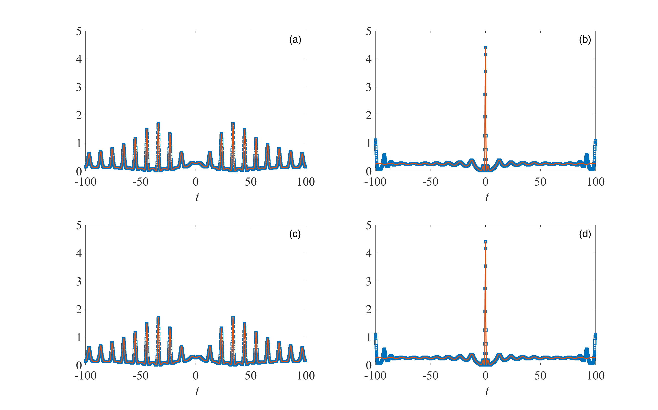
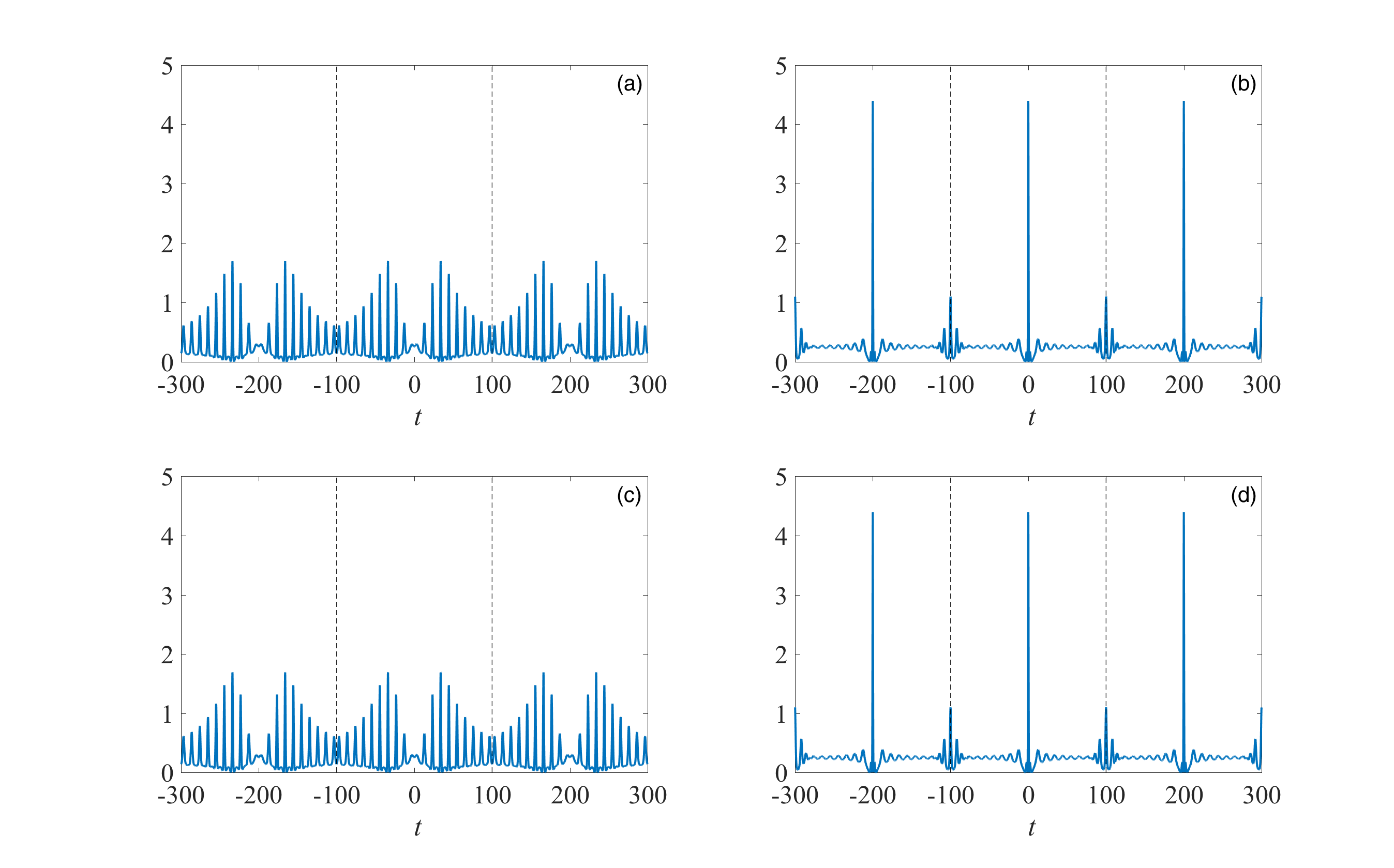
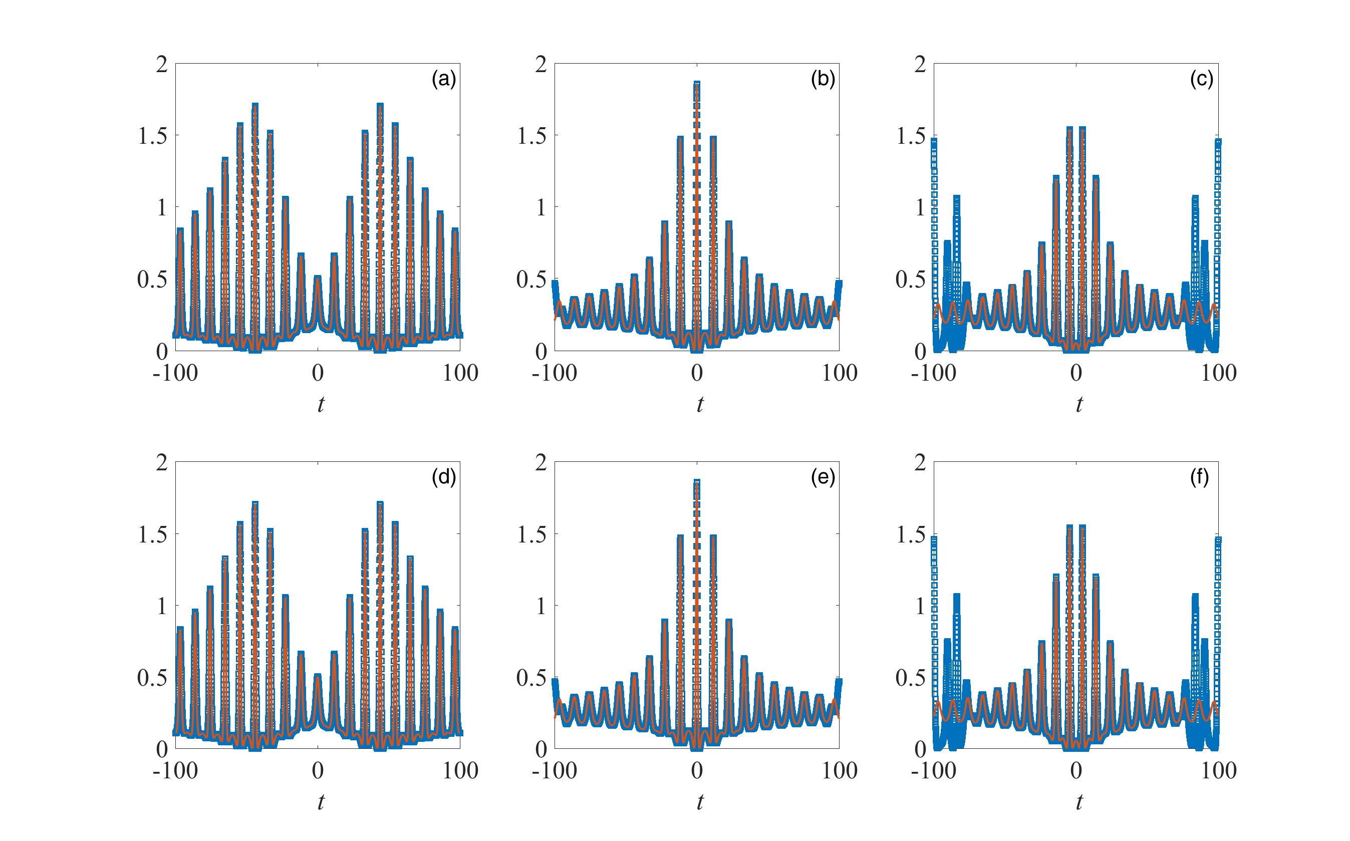
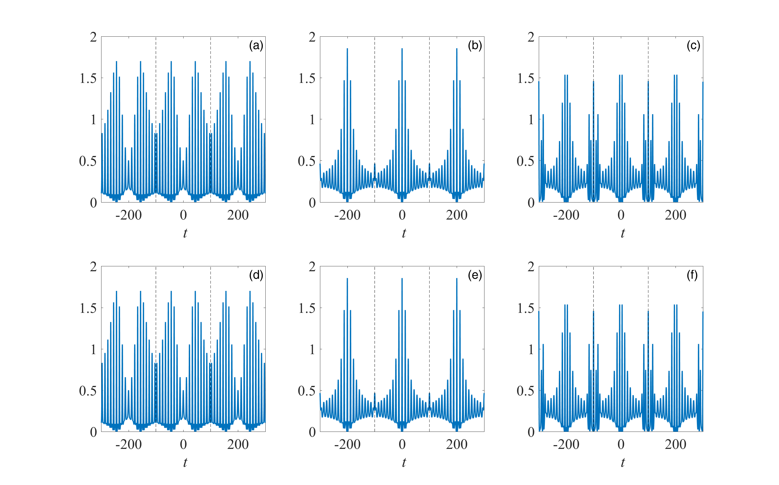
Figures (17,19) are simulated numerically for fundamental and triangular patterns of the order-2 b-positon with . Because of the feature of the frequency comb system and wave shaper, the input pulse will be a periodic time series [50], figures (18,20) are simulated numerically for the periodic extension of above two cases, which can provide useful information for experiments. The curves are not recognizable if we also put theoretical results in figures (18,20) because the theoretical results almost coincide completely with the numerical simulations, so we do not add them here.
We find that there is an excellent agreement between theoretical (and exact) results and numerical simulations when SNR 100, which shows these solutions have strong robustness to the unavoidable noise at high SNR in the optical fiber. The significant discrepancies between theoretical and numerical results occur at the two ends of period due to the reflection of simulation. This discrepancy is reducible by increasing the period of simulation. Therefore the fundamental and triangular patterns in order-2 b-positon are available in realistic optical fiber system even there exists a strong noise. These results strongly indicating the possible observation of the higher-order rogue waves by using the central patterns of the b-positons in optical fibre systems.
As we have pointed out in section IV that, in order to get more accurate approximation of the higher-order rogue waves, it is better to set of the b-positons to be more closer to . In other words, we could consider that the b-positon is more closer to the rogue wave in experiment. However, the rogue wave is extremely unstable, and thus the b-positon with the inclusion of noise becomes gradually but strongly unstable when is approaching . Therefore, it is difficult to observe the b-positon when it is very close to the rogue wave in experiments, not to mention the rogue wave. The numerical simulations in figure 21 is clearly shows the increasing trend of the instability when is approaching , which can be seen from the additional small peaks appeared in ()-plane. Furthermore, the -shape profile of the peaks are destroyed gradually in panels by the noise from top to bottom in figure 21. Finally, the main peak of rogue wave (see bottom of the same figure) is not recognizable because it is fully surrounded by noise peaks.
VI Conclusions
In conclusion, we have introduced the so-called b-positon of the NLS equation, which is obtained by taking the limit in an order- breather. In other words, an order- b-positon is given by single breathers with same height and period. We have provided a formula expressed by the determinants and the higher-order Taylor expansion in eq.(10). It converts into an order- rogue wave by further limit . Here is a special eigenvalue in a single breather of the NLS such that its period goes to infinity, and then this breather becomes a order-1 rogue wave. We have plotted up to the order-5 b-positons in figures 2-6. Based on analytical formulas, we have presented a sketchy demonstration of the two limits from an order-2 breather to an order-2 rogue wave in figures 1-3. In order to show the wide applicability of order-n b-positon in eq.(10), we also plotted the tilted propagation of the higher-order b-positons in figures 12-14.
There are two main advantages of the b-positon, i.e., a convenient conversion to the rogue wave and the easy controllability of the patterns in the central region in the ()-plane. Thus, we have suggested a new way to observe the higher-order rogue waves, namely, observe the profiles of the central region of the higher-order b-positon when is very close to the , which can be done in an optical fiber system given by figure 1 in ref. [49] or figure 3 in ref.[50]. The ideal initial input pulse is created by a frequency comb system and a programable optical filter(wave shaper) according to the profile of an analytical form of the b-positon at a certain position . We have also plotted the theoretically predicted output pulses in figures 7-11, which are useful to observe the higher-order rogue waves in fiber according to suggested approach in this paper. Three patterns associated with above output pulses are plotted in figures 15 and 16.
The excellent agreements between theoretical and numerical simulation results in figures 17-20, and the tendency of the instability for the b-positons in figure 21 support strongly our above new approach to observe the b-positons in a realistic optical fiber system. Our results also show the validity of the generating mechanism of a higher-order rogue wave from the double degeneracy of a multi-breather.
Acknowledgments. This work is supported by the NSF of China under Grant No. 11671219, and the K.C. Wong Magna Fund in Ningbo University. This study is also supported by the open Fund of the State Key Laboratory of Satellite Ocean Environment Dynamics, Second Institute of Oceanography(No. SOED1708). K. P. thanks the IFCPAR,DST, NBHM, and CSIR, Government of India, for the financial support through major projects.
VII Figures
VII.1 Breathers and bpostions


VII.2 Ideal initial input pulses and predicted output pulses


| 12.89 | 23.38 | 33.87 | 44.36 | 54.85 | 65.33 | 75.82 | 86.30 | 96.78 | 107.25 | |
|---|---|---|---|---|---|---|---|---|---|---|
| 0.66 | 1.32 | 1.69 | 1.47 | 1.16 | 0.93 | 0.78 | 0.68 | 0.61 | 0.56 | |
| 10.48 | 10.49 | 10.49 | 10.49 | 10.48 | 10.48 | 10.48 | 10.48 | 10.48 |
Notes: , denotes the time of a peak, denotes the amplitude of a peak.


| 11.69 | 22.65 | 33.36 | 43.96 | 54.53 | 65.06 | 75.58 | 86.09 | 96.59 | 107.08 | |
|---|---|---|---|---|---|---|---|---|---|---|
| 0.66 | 1.053 | 1.513 | 1.701 | 1.564 | 1.33 | 1.11 | 0.95 | 0.83 | 0.74 | |
| 10.96 | 10.70 | 10.61 | 10.56 | 10.53 | 10.52 | 10.51 | 10.50 | 10.50 |
Notes: , denotes the time of a peak, denotes the amplitude of a peak.


| 15.16 | 25.63 | 36.15 | 46.67 | 57.18 | 67.69 | 78.20 | 88.70 | 99.19 | 109.69 | |
|---|---|---|---|---|---|---|---|---|---|---|
| 0.37 | 0.87 | 1.70 | 1.12 | 0.69 | 0.51 | 0.43 | 0.38 | 0.35 | 0.33 | |
| 10.48 | 10.51 | 10.52 | 10.51 | 10.51 | 10.50 | 10.50 | 10.50 | 10.49 |
Notes: , denotes the time of a peak, denotes the amplitude of a peak.


| 13.10 | 24.34 | 35.20 | 45.92 | 56.56 | 67.16 | 77.73 | 88.29 | 98.83 | 109.35 | |
|---|---|---|---|---|---|---|---|---|---|---|
| 0.46 | 0.97 | 1.72 | 1.26 | 0.79 | 0.57 | 0.47 | 0.41 | 0.37 | 0.34 | |
| 11.24 | 10.87 | 10.72 | 10.64 | 10.60 | 10.57 | 10.55 | 10.54 | 10.53 |
Notes:, denotes the time of a peak, denotes the amplitude of a peak.
| 2.12 | 14.49 | 25.41 | 36.04 | 46.60 | 57.14 | 67.66 | 78.17 | 88.68 | 99.18 | |
|---|---|---|---|---|---|---|---|---|---|---|
| 0.30 | 0.40 | 0.93 | 1.71 | 1.08 | 0.67 | 0.50 | 0.42 | 0.37 | 0.34 | |
| 12.33 | 10.93 | 10.62 | 10.56 | 10.54 | 10.52 | 10.51 | 10.51 | 10.50 |
Notes: , denotes the time of a peak, denotes the amplitude of a peak.


VIII Appendix
VIII.1 Rogue waves
VIII.1.1 Order-1 Rogue wave
Taking the limit , the single breather yields the firsr-order rogue wave
| (11) |
with
VIII.1.2 Order-2 Rogue wave
Taking the limit and setting , order-2 b-positon yields an order-2 rogue wave
| (12) |
Here
denotes the real part, denotes the imaginary part.
VIII.2 b-positons (order-2 and order-3)
VIII.2.1 Order-2 Bpositons
Set and in , an order-2 b-positon is given by
Here
and
VIII.2.2 Order-3 Bpositons with Fundamental pattern
Set and in , an order-3 b-positon is given by
VIII.3 The tilted propagation of the b-positons (order-2 and order-3)


VIII.4 B-positons(order-2 and order-3) for experiments


VIII.5 Numerical simulations for order-2 b-positons
The numerical code for the NLS equation is given in ref.[20](see its appendix B). In following figures, the first column denotes input signals, others denote output signals.
VIII.6 The demonstration of instability for the order-2 b-positon by numerical simulation
In this appendix, we use numerical figures to show the increasing trend of the instability for the order-2 b-positon when .


References
- [1] R. Y. Chiao, E. Garmire, and C. H. Townes, Self-trapping of optical beams, Phys. Rev. Lett. 13, 479–482 (1964).
- [2] V. E. Zakharov, S. V. Manakov, S. P. Novikov, and L. P. Pitaevskii, Theory of Solitons: the Inverse Scattering Method (Nauka Publishers: Moscow,198-).
- [3] M. J. Ablowitz and P. A. Clarkson, Solitons, Nonlinear Evolution Equations and Inverse Scattering (Cambridge University Press, Cambridge, UK, 1991).
- [4] A. Hasegawa and F. Tappert, Transmission of stationary nonlinear optical pulses in dispersive dielectric fibers. I: Anomalous dispersion, Appl. Phys. Lett. 23, 142–144 (1972).
- [5] A. Hasegawa and F. Tappert, Transmission of stationary nonlinear optical pulses in dispersive dielectric fibers. II: Normal dispersion, Appl. Phys. Lett. 23, 171–172 (1973).
- [6] L. F. Mollenauer, R. H. Stolen, and J. P. Gordon, Experimental Observation of Picosecond Pulse Narrowing and Solitons in Optical Fibers, Phys. Rev. Lett. 45, 1095–1098 (1980).
- [7] S. Maneuf, R. Desailly, and C. Froehly, Stable self-trapping of laser beams: Observation in a nonlinear planar waveguides, Opt. Commun. 65, 193 (1988).
- [8] B. A. Malomed, D. Mihalache, F. Wise, and L. Torner, Spatiotemporal optical solitons, J. Opt. B 7, R53–R72 (2005).
- [9] Y. V. Kartashov, B. A. Malomed, and L. Torner, Solitons in nonlinear lattices, Rev. Mod. Phys. 83, 247–305 (2011).
- [10] P. Grelu and N. Akhmediev, Dissipative solitons for mode-locked lasers, Nature Phot. 6, 84–92 (2012).
- [11] D. Mihalache, Linear and nonlinear light bullets: Recent theoretical and experimental studies, Rom. J. Phys. 57, 352–371 (2012).
- [12] Z. G. Chen, M. Segev, and D. Christodoulides, Optical spatial solitons: historical overview and recent advances, Rep. Prog. Phys. 75, 086401 (2012).
- [13] H. Leblond and D. Mihalache, Models of few optical cycle solitons beyond the slowly varying envelope approximation, Phys. Rep. 523, 61–126 (2013).
- [14] B. A. Malomed, Spatial solitons supported by localized gain, J. Opt. Soc. Am. B 31, 2460–2475 (2014).
- [15] D. J. Frantzeskakis, H. Leblond, and D. Mihalache, Nonlinear optics of intense few-cycle pulses: An overview of recent theoretical and experimental developments, Rom. J. Phys. 59, 767–784 (2014).
- [16] M. Tlidi, K. Staliunas, K. Panajotov, A. G. Vladimirov, and M. G. Clerc, Introduction – Localized structures in dissipative media: from optics to plant ecology, Phil. Trans. R. Soc. A 372, 20140101 (2014).
- [17] D. Mihalache, Localized structures in nonlinear optical media: a selection of recent studies, Rom. Rep. Phys. 67, 1383–1400 (2015).
- [18] A. Hasegawa and Y. Kodama, Solitons in Optical Communications (Oxford University Press, Oxford, 1995).
- [19] Y. S. Kivshar and G. Agrawal, Optical Solitons: From Fibers to Photonic Crystals (Academic Press, San Diego, 2003).
- [20] G. Agrawal, Nonlinear Fiber Optics(Fifth Edition)(Academic Press, Oxford, 2013).
- [21] D. H. Peregrine, Water waves, nonlinear Schrödinger equations and their solutions, J. Austral. Math. Soc. B 25, 16–43 (1983).
- [22] N. Akhmediev, M. M. Eleonskii, and N. E. Kulagin, Generation of a Periodic Sequence of Picosecond Pulses in an Optical Fibre: Exact solutions, Sov. Phys. JETP 62, 894–899 (1985).
- [23] E. A. Kuznetsov, Solitons in a parametrically unstable plasma, Sov. Phys. Doklady 22, 507–508 (1977).
- [24] Y. C. Ma, The perturbed plane-wave solutions of the cubic Schrödinger equation. Stud. Appl. Math. 60, 43–58 (1979).
- [25] N. Akhmediev and V. I. Korneev, Modulation instability and periodic solutions of the nonlinear Schrödinger equation, Theor. Math. Phys. 69, 1089–1093 (1986).
- [26] A. Chabchoub, N. P. Hoffmann, and N. Akhmediev, Rogue Wave Observation in a Water Wave Tank, Phys. Rev. Lett. 106, 204502 (2011).
- [27] A. Chabchoub, N. Hoffmann, M. Onorato, and N. Akhmediev, Super Rogue Waves: Observation of a Higher-Order Breather in Water Waves, Phys. Rev. X 2, 011015(2012).
- [28] A. Chabchoub,N. Hoffmann, M. Onorato, A. Slunyaev, A. Sergeeva, E. Pelinovsky, and N. Akhmediev, Observation of a hierarchy of up to fifth-order rogue waves in a water tank, Phys. Rev. E. 86, 056601(2012).
- [29] A. Chabchouba, N. Akhmediev, Observation of rogue wave triplets in water waves, Phys. Lett. A 377, 2590-2593(2013).
- [30] A. Chabchoub, M. Fink, Time-Reversal Generation of Rogue Waves, Phys. Rev. Lett. 112, 124101(2014).
- [31] B. Kibler, J. Fatome, C. Finot, G. Millot, F. Dias, G. Genty, N. Akhmediev, and J. M. Dudley, The Peregrine soliton in nonlinear fibre optics, Nat. Phys. 6, 790–795 (2010).
- [32] K. Hammani, B. Kibler, C. Finot, P. Morin, J. Fatome, J. M. Dudley, and G. Millot, Peregrine soliton generation and breakup in standard telecommunications fiber, Opt. Lett. 36, 112–114 (2011).
- [33] B. Kibler, J. Fatome, C. Finot, G. Millot, G. Genty, B. Wetzel, N. Akhmediev, F. Dias, and J. M. Dudley, Observation of Kuznetsov-Ma soliton dynamics in optical fibre, Sci. Rep. 2, 463 (2012).
- [34] B. Frisquet, B. Kibler, P. Morin, F. Baronio, M. Conforti, and B. Wetzel, Optical dark rogue wave, Sci. Rep. 6, 20785 (2016).
- [35] J. S. He, H. R. Zhang, L. H. Wang, K. Porsezian, and A. S. Fokas, Generating mechanism for higher-order rogue waves, Phys. Rev. E 87, 052914 (2013).
- [36] D. J. Kedziora, A. Ankiewicz, and N. Akhmediev, Circular rogue wave cluster, Phys. Rev. E 84,056611(2011)
- [37] N. Akhmediev, J. M. Soto-Crespo, and A. Ankiewicz, Extreme waves that appear from nowhere: On the nature of rogue waves, Phys. Lett. A 373, 2137–2145 (2009).
- [38] N. Akhmediev, J. M. Soto-Crespo, and A. Ankiewicz, How to excite a rogue wave, Phys. Rev. A. 80, 043818(2009).
- [39] D. J. Kedziora, A. Ankiewicz, and N. Akhmediev, Classifying the hierarchy of nonlinear-Schrödinger-equation rogue-wave solutions, Phys. Rev. E 88, 013207(2013).
- [40] D. J. Kedziora, A. Ankiewicz, and N. Akhmediev, Second-order nonlinear-Schrödinger-equation breather solutions in the degenerate and rogue wave limits, Phys. Rev. E 85, 066601(2012).
- [41] V. B. Matveev and M. A. Salle, Darboux Transformations and Solitons (Springer-Verlag, Berlin), 1991.
- [42] J. S. He, L. Zhang, Y. Cheng, and Y. S. Li, Determinant representation of Darboux transformation for the AKNS system, Science in China Series A: Mathematics 49, 1867–1878 (2006).
- [43] J. S. He, M. Ji, and Y. S. Li, Solutions of two kinds of non-isospectral generalized nonlinear Schrödinger equation related to Bose-Einstein condensates, Chinese Phys. Lett. 24, 2157–2160 (2007).
- [44] L. Zhang, J. S. He, Y. Cheng, and Y. S. Li, Surfaces and Curves Corresponding to the Solutions Generated from Periodic Seed of NLS Equation, Acta Mathematica Sinica (English Series) 28, 1713–1726 (2012).
- [45] V. B. Matveev, Generalized Wronskian formula for solutions of the KdV equations: first applications, Phys. Lett. A 166, 205-208(1992).
- [46] V. B. Matveev, Positon-positon and soliton-positon collisions: KdV case, Phys. Lett. A 166, 209-212(1992).
- [47] See Supplemental Material at \textcolorred[URL will be inserted by publisher] for the analytical demonstration of double degeneracy. Four animations demonstrate clearly the tendency from a breather to a b-positon, and then to a rogue wave. Specifically, breather2bp0.gif shows the transferring from a breather to a b-positon with a fundamental pattern; breather2bp1.gif shows the transferring from a breather to a b-positon with a triangular pattern; bp2rw0.gif shows the transferring from a b-positon to a rogue wave with a fundamental pattern; bp2rw1.gif shows the transferring from a b-positon to a rogue wave with a triangular pattern.
- [48] B. Frisquet, B. Kibler, and G. Millot, Collision of Akhmediev Breathers in Nonlinear Fiber Optics, Phys. Rev. X 3, 041032 (2013).
- [49] B. Frisquet, A. Chabchoub, J. Fatome, C. Finot, B. Kibler, and G. Millot, Two-stage linear-nonlinear shaping of an optical frequency comb as rogue nonlinear-Schrödinger-equation-solution generator, Phys. Rev. A 89, 023821(2014).
- [50] B. Kibler, A. Chabchoub, A. Gelash, N. Akhmediev, and V. E. Zakharov, Superregular Breathers in Optics and Hydrodynamics: Omnipresent Modulation Instability beyond Simple Periodicity, Phys. Rev. X 5, 041026(2015).
- [51] A. A. Gelash and V. E. Zakharov, Superregular solitonic solutions: a novel scenario for the nonlinear stage of modulation instability, Nonlinearity 27, R1-R39 (2014).