Deep Learning and Quantum Entanglement:
Fundamental Connections with Implications to Network Design

We provide below minimal background on tensors which is sufficient to follow the definitions and arguments of this paper. For a comprehensive introduction it is worthwhile to refer to Hackbusch (2012). The core concept in tensor analysis is a tensor, which may be thought of as a multi-dimensional array. The order of a tensor is defined to be the number of indexing entries in the array, which are referred to as modes. The dimension of a tensor in a particular mode is defined as the number of values that may be taken by the index in that mode. If ${\mathcal{A}}$ is a tensor of order $N$ and dimension $M_{i}$ in each mode $i\in[N]:=\{1,\ldots,N\}$, the space of all configurations it can take is denoted, quite naturally, by ${\mathbb{R}}^{M_{1}{\times\cdots\times}M_{N}}$.

An important concept we will make use of is matricization, which is essentially the rearrangement of a tensor as a matrix. Suppose ${\mathcal{A}}$ is a tensor of order $N$ and dimension $M_{i}$ in each mode $i\in[N]$, and let $(I,J)$ be a partition of $[N]$, i.e. $I$ and $J$ are disjoint subsets of $[N]$ whose union gives $[N]$. We may write $I=\{i_{1},\ldots,i_{\left\lvert I\right\rvert}\}$ where $i_{1}<\cdots<i_{\left\lvert I\right\rvert}$, and similarly $J=\{j_{1},\ldots,j_{\left\lvert J\right\rvert}\}$ where $j_{1}<\cdots<j_{\left\lvert J\right\rvert}$. The matricization of ${\mathcal{A}}$ w.r.t. the partition $(I,J)$, denoted $\llbracket{\mathcal{A}}\rrbracket_{I,J}$, is the $\prod_{t=1}^{\left\lvert I\right\rvert}M_{i_{t}}$-by-$\prod_{t=1}^{\left\lvert J\right\rvert}M_{j_{t}}$ matrix holding the entries of ${\mathcal{A}}$ such that ${\mathcal{A}}_{d_{1}{\ldots}d_{N}}$ is placed in row index $1+\sum_{t=1}^{\left\lvert I\right\rvert}(d_{i_{t}}-1)\prod_{t^{\prime}=t+1}^{\left\lvert I\right\rvert}M_{i_{t^{\prime}}}$ and column index $1+\sum_{t=1}^{\left\lvert J\right\rvert}(d_{j_{t}}-1)\prod_{t^{\prime}=t+1}^{\left\lvert J\right\rvert}M_{j_{t^{\prime}}}$.

A fundamental operator in tensor analysis is the tensor product, which we denote by $\otimes$. It is an operator that intakes two tensors ${\mathcal{A}}\in{\mathbb{R}}^{M_{1}{\times\cdots\times}M_{P}}$ and ${\mathcal{B}}\in{\mathbb{R}}^{M_{P+1}{\times\cdots\times}M_{P+Q}}$ (orders $P$ and $Q$ respectively), and returns a tensor ${\mathcal{A}}\otimes{\mathcal{B}}\in{\mathbb{R}}^{M_{1}{\times\cdots\times}M_{P+Q}}$ (order $P+Q$) defined by: $({\mathcal{A}}\otimes{\mathcal{B}})_{d_{1}{\ldots}d_{P+Q}}={\mathcal{A}}_{d_{1}{\ldots}d_{P}}\cdot{\mathcal{B}}_{d_{P+1}{\ldots}d_{P+Q}}$. Notice that in the case $P=Q=1$, the tensor product reduces to the standard outer product between vectors, i.e. if ${\mathbf{u}}\in{\mathbb{R}}^{M_{1}}$ and ${\mathbf{v}}\in{\mathbb{R}}^{M_{2}}$, then $K={\mathbf{u}}\otimes{\mathbf{v}}$ is no other than the rank-$1$ matrix $K={\mathbf{u}}{\mathbf{v}}^{\top}\in{\mathbb{R}}^{M_{1}{\times}M_{2}}$, whose entries hold the value: $K_{ij}=u_{i}v_{j}$. A generalization to the tensor product of $N$ vectors ${\mathbf{v}}^{(j)}\in{\mathbb{R}}^{M_{j}}$ for $j\in[N]$, results in an order $N$ tensor ${\mathcal{A}}_{d_{1}...d_{N}}^{\textrm{(rank 1)}}={\mathbf{v}}^{(1)}\otimes\cdots\otimes{\mathbf{v}}^{(N)}$, whose entries hold the values:

Tensors of this form are regarded as having rank-$1$ (assuming ${\mathbf{v}}^{(j)}\neq 0~~\forall j$).

Our construction will relate to the convolutional arithmetic circuit (ConvAC) architecture introduced by Cohen et al. (2016b). The ConvAC network, illustrated in fig. 1, is a deep convolutional network that operates exactly as a regular ConvNet, only with linear activations and product pooling layers (which introduce the non-linearity) instead of the more common non-linear activations (e.g. ReLU) and average/max pooling. From an empirical perspective, ConvACs work well in many practical settings, e.g. for optimal classification with missing data (Sharir et al. (2016)), and for compressed networks (Cohen et al. (2016a)). Furthermore, their underlying operations lend themselves to mathematical analyses based on measure theory and tensor analysis — the depth efficiency of deep convolutional networks was shown using this framework. Importantly, through the concept of generalized tensor decompositions, ConvACs can be transformed to standard ConvNets with ReLU activations and average/max pooling, which laid the foundation for extending its proof methodologies to general ConvNets (Cohen and Shashua (2016)). This deep learning architecture was chosen for our analysis below due to its underlying tensorial structure which resembles the quantum many-body wave function, as we show in sec. 3.

In the ConvAC architecture (see fig. 1), each point in the input space of the network, denoted by $X=({\mathbf{x}}_{1},\ldots,{\mathbf{x}}_{N})$, is represented as an $N$-length sequence of $s$-dimensional vectors ${\mathbf{x}}_{1},\ldots,{\mathbf{x}}_{N}\in{\mathbb{R}}^{s}$. $X$ is typically thought of as an image, where each ${\mathbf{x}}_{j}$ corresponds to a local patch from that image and $s$ is the number of pixels in each patch. The first layer of the network is referred to as the representation layer, which involves the application of $M$ representation functions $f_{\theta_{1}},\ldots,f_{\theta_{M}}:{\mathbb{R}}^{s}\to{\mathbb{R}}$ on each local patch ${\mathbf{x}}_{j}$, giving rise to $M$ feature maps. Under the common setting, where the representation functions are selected to be $f_{\theta_{d}}({\mathbf{x}})=\sigma({\mathbf{w}}_{d}^{T}{\mathbf{x}}+b_{d})$ for some point-wise activation $\sigma(\cdot)$ and parameterized by $\theta_{d}=({\mathbf{w}}_{d},b_{d})\in{\mathbb{R}}^{s}\times{\mathbb{R}}$, the representation layer reduces to the standard convolutional layer. Other possibilities, e.g. gaussian functions with diagonal covariances, have also been considered in Cohen et al. (2016b). Following the representation layer, are hidden layers indexed by $l=0,\ldots,L-1$, each beginning with a $1\times 1$ conv operator, which is just an $r_{l-1}\times 1\times 1$ convolutional layer with $r_{l-1}$ input channels and $r_{l}$ output channels. Following each conv layer is a spatial pooling, that takes products of non-overlapping two-dimensional windows covering the output of the previous layer, where for $l=L-1$ the pooling window is the size of the entire spatial dimension (i.e. global pooling), reducing its output’s shape to a $r_{L-1}\times 1\times 1$, i.e. an $r_{L-1}$-dimensional vector. The final $L$ layer maps this vector with a dense linear layer into the $Y$ network outputs, denoted by ${\mathbf{h}}_{y}({\mathbf{x}}_{1},\ldots,{\mathbf{x}}_{N})$, representing score functions classifying each $X$ to one of the classes through: $y^{*}=\argmax_{y}{\mathbf{h}}_{y}({\mathbf{x}}_{1},\ldots,{\mathbf{x}}_{N})$. As shown in Cohen et al. (2016b), these functions have the following form:

where ${\mathcal{A}}^{y}$, called the convolutional weights tensor, is a tensor of order $N$ and dimension $M$ in each mode, with entries given by polynomials in the network’s convolutional weights.

Several decompositions of the convolutional weights tensor were introduced in previous works. Any tensor can be expressed as a sum of rank-$1$ tensors, and the decomposition of ${\mathcal{A}}$ in such a manner is referred to as the CANDECOMP/PARAFAC decomposition of ${\mathcal{A}}$, or in short the CP decomposition. This corresponds to a network such as depicted in fig.  1 with one hidden layer collapsing the entire spatial structure through global pooling. Another decomposition which was shown to be universal, is the Hierarchical Tucker tensor decomposition which we refer to in short as HT decomposition. A restricted version of this decomposition (which includes same channel pooling; to be presented more thoroughly below), corresponds to a network such as depicted in fig.  1 with $L=\log_{4}N$ hidden layers which pool over size-$2\times 2$ windows. This deep convolutional network was shown to have an exponential advantage in expressiveness over the shallow one realizing the CP decomposition (Cohen et al. (2016b)) (our analysis below reproduces this result as a by-product, see sec. 7.4). We will discuss such tensors decompositions extensively in sec. 5.2 as we will tie them to Tensor Networks, a tool used by physicists when describing many-body quantum wave functions, leading us to the main results of this work.

Finally, it is instructive for our purposes to define $N$ vectors ${\mathbf{v}}^{(j)}\in{\mathbb{R}}^{M}$ for $j\in[N]$ that hold the values $v_{d}^{(j)}=f_{\theta_{d}}({\mathbf{x}}_{j})$ for $d\in[M]$. This construction implies that the result of applying the $d^{th}$ representation function on the $j^{th}$ image patch is stored in the $d^{th}$ entry of ${\mathbf{v}}^{(j)}$. Using the form of the rank $1$ tensor presented in eq. 1, the score functions may then be written as:

where as described above, ${\mathcal{A}}_{d_{1}...d_{N}}^{\textrm{(rank 1)}}({\mathbf{x}}_{1},\ldots,{\mathbf{x}}_{N})$ is obtained by applying the representation functions on the input patches and ${\mathcal{A}}^{y}_{d_{1}...d_{N}}$ represents the network’s convolutional weights.

In a way, ConvACs form a bridge between ConvNets and TNs as they are described using the language of tensors, similarly to TNs. The tensor language underlying ConvACs is based on rank decompositions through linear combinations of outer-products of low-order tensors (see sec. 5.2) whereas TNs are described by contractions over low-order tensors (sec. 5.1). Before we can make this connection, we describe below the quantum mechanical language necessary to map between the two worlds, and show a structural equivalence between ConvACs and many-body wave functions.

A state of a system, which is a complete description of a physical system, is given in quantum mechanics as a ray in a Hilbert space (to be defined below). Relevant Hilbert spaces in quantum mechanics are vector spaces over the complex numbers. We will restrict our discussion to vector spaces over ${\mathbb{R}}$, as the properties related to complex numbers are not required for our analysis and do not affect it. Physicists denote such vectors in the ‘ket’ notation, in which a vector $\psi$ is denoted by: $\left|\psi\right\rangle\in{\cal H}$. The Hilbert space ${\cal H}$ has an inner product denoted by $\left\langle\phi|\psi\right\rangle$, that maps a pair of two vectors in ${\cal H}$ to a scalar. This inner product operation is also referred to as ‘projecting $\left|\psi\right\rangle$ onto $\left|\phi\right\rangle$’. A ray is an equivalence class of vectors that differ by multiplication by a nonzero scalar. For any nonzero ray, a representative of the class, $\left|\psi\right\rangle$, is conventionally chosen to have a unit norm: $\left\langle\psi|\psi\right\rangle=1$. A ‘bra’ notation $\left\langle\phi\right|$, is used for the ‘dual vector’ which formally is a linear mapping between vectors to scalars defined as $\left|\psi\right\rangle\mapsto\left\langle\phi|\psi\right\rangle$. We can intuitively think of a ‘ket’ as a column vector and ‘bra’ as a row vector.

Relevant Hilbert spaces can be infinite dimensional or finite dimensional. We will limit our discussion to quantum states which reside in finite dimensional Hilbert spaces, as eventually these will be at the heart of our analogy to convolutional networks. Besides being of interest to us, these spaces are extensively investigated in the physics community as well. For example, the spin component of a spinful particle’s wave function resides in a finite dimensional Hilbert space. One can represent a general state $\left|\psi\right\rangle\in\cal H$, where $\textrm{dim}({\cal H})=M$, as a linear combination of some orthonormal basis vectors:

where ${\mathbf{v}}\in\mathbb{R}^{M}$ is the vector of coefficients compatible with the basis $\{\left|\psi_{d}\right\rangle\}_{d=1}^{M}$ of $\cal H$, each entry of which can be calculated by the projection: $v_{d}=\left\langle\psi_{d}|\psi\right\rangle$.

The extension to the case of $N$ particles, each with a wave function residing in a local finite dimensional Hilbert space ${\cal{H}}_{j}$ for $j\in[N]$ (e.g. $N$ spinful particles), is readily available through the tool of a tensor product. In order to define a Hilbert space which is the tensor product of the local Hilbert spaces: ${\cal H}:=\otimes_{j=1}^{N}{\cal{H}}_{j}$, we will specify its scalar product. Denote the scalar product in ${\cal{H}}_{j}$ by $\left\langle\cdot|\cdot\right\rangle_{j}$, then the scalar product of the finite dimensional Hilbert space ${\cal H}=\otimes_{j=1}^{N}{\cal{H}}_{j}$ between $\left|\psi\right\rangle:=\otimes_{j=1}^{N}\left|\psi^{(j)}\right\rangle\in{\cal H}$ and $\left|\phi\right\rangle:=\otimes_{j=1}^{N}\left|\phi^{(j)}\right\rangle\in{\cal H}$ is defined by: $\left\langle\phi|\psi\right\rangle:=\prod_{j=1}^{N}\left\langle\phi^{(j)}|\psi^{(j)}\right\rangle_{j}~,~\forall\left|\psi^{(j)}\right\rangle,\left|\phi^{(j)}\right\rangle\in{\cal{H}}_{j}$.

For simplicity, we set the dimensions of the local Hilbert spaces ${\cal{H}}_{j}$ to be equal for all $j$, i.e. $\forall j:\textrm{dim}({\cal{H}}_{j})=M$. Physically, this means that the particles have the same spin, e.g. for $N$ electrons (spin $1/2$), $M=2$. Denoting the orthonormal basis of the local Hilbert space by $\{\left|\psi_{d}\right\rangle\}_{d=1}^{M}$, the many-body quantum wave function $\left|\psi\right\rangle\in{\cal H}=\otimes_{j=1}^{N}{\cal{H}}_{j}$ can be written as:

where $\left|\psi_{d_{1}}\right\rangle\otimes\cdots\otimes\left|\psi_{d_{N}}\right\rangle$ is a basis vector of the $M^{N}$ dimensional Hilbert space ${\cal H}$, and $\mathcal{A}_{d_{1}...d_{N}}$ is the tensor holding the corresponding coefficients.

We will tie between the function realized by a ConvAC, given in eqs. 2 and 3, and the many-body quantum wave function given in eq. 5. First, we consider a special case of $N$ particles which exhibit no quantum correlations (to be formulated in sec. 4 below). The state of such a system is called a product state, and can be written down as a single tensor product of local states $\left|\phi_{j}\right\rangle\in{\cal{H}}_{j}$: $\left|\psi^{~\textrm{ps}}\right\rangle=\left|\phi_{1}\right\rangle\otimes\cdots\otimes\left|\phi_{N}\right\rangle$. Let $\{\left|\psi_{d_{j}}\right\rangle\}_{d_{j}=1}^{M}$ be an orthonormal basis for ${\cal{H}}_{j}$. By expanding each local state in this basis:

the product state assumes a form similar to eq. 5:

with the underlying rank $1$ coefficients tensor ${\mathcal{A}}^{~\textrm{ps}}_{d_{1}...d_{N}}=\prod_{j=1}^{N}v^{(j)}_{d_{j}}$. In a similar construction as one presented in sec 2.2, if we compose each local state $\left|\phi_{j}\right\rangle$ s.t. its projection on the local basis vector would equal $v_{d}^{(j)}=\left\langle\psi_{d}|\phi_{j}\right\rangle=f_{\theta_{d}}({\mathbf{x}}_{j})$, then the projection of the many-body quantum state $\left|\psi\right\rangle$ onto the product state $\left|\phi\right\rangle$ is equal to¹¹ 1 The bases were chosen to be orthonormal and the representation functions are only linearly independent and not necessarily orthogonal. Similar to the argument presented in Cohen and Shashua (2017), as the linear independence of the representation functions implies that the dimension of $span\{f_{\theta_{1}}{\ldots}f_{\theta_{M}}\}$ is $M$, upon transformation of the conv weights in hidden layer $0$ the overall function ${\mathbf{h}}_{y}$ remains unchanged. :

reproducing eqs. 2 and 3 for a single class $y$, as ${\mathcal{A}}^{~\textrm{ps}}_{d_{1}...d_{N}}={\mathcal{A}}^{~\textrm{(rank 1)}}_{d_{1}...d_{N}}$ by construction. This result ties between the function realized by a convolutional network to that which a many-body wave function models. Specifically, the tensor holding the convolutional weights is analogous to the coefficients tensor of the many-body wave function, while the input to the convolutional network is analogous to the constructed separable state. In the following sections, we will use this analogy to acquire means of describing and analyzing the expressiveness of the convolutional network via properties of its underlying tensor.

Physical correlations are discussed in several related contexts. Here, we will focus on a type of correlation referred to as quantum entanglement²² 2 Besides discussing the quantum entanglement that characterizes the wave function itself, physicists describe related correlations via the concept of quantum operators, which we did not introduce here for conciseness.. Consider a partition of the above described system of $N$ particles labeled by integers $[N]:=\{1,\ldots,N\}$, which splits it into two disjoint subsystems $A\mathbin{\mathaccent 0{\cdot}\cup}B=[N]$ such that $A=\{a_{1},\ldots,a_{|A|}\}$ with $a_{1}<...<a_{|A|}$ and $B=\{b_{1},\ldots,b_{|B|}\}$ with $b_{1}<...<b_{|B|}$. Let ${\cal{H}}^{A}$ and ${\cal{H}}^{B}$ be the Hilbert spaces in which the many-body wave functions of the particles in subsystems $A$ and $B$ reside, respectively, with ${\cal H}={\cal{H}}^{A}\otimes{\cal{H}}^{B}~$³³ 3 Actually, ${\cal H}\cong{\cal{H}}^{A}\otimes{\cal{H}}^{B}$ with equality obtained upon a permutation of the local spaces that is compliant with the partition $(A,B)$. . The many-body wave function in eq. 5 can be now written as:

where $\{\left|\psi_{\alpha}^{A}\right\rangle\}_{\alpha=1}^{\textrm{dim}({\cal{H}}^{A})}$ and $\{|\psi_{\beta}^{B}\rangle\}_{\beta=1}^{\textrm{dim}({\cal{H}}^{B})}$ are bases for ${\cal{H}}^{A}$ and ${\cal{H}}^{B}$, respectively⁴⁴ 4 It is possible to write $\left|\psi_{\alpha}^{A}\right\rangle=\left|\psi_{d_{a_{1}}}\right\rangle\otimes\cdots\otimes|\psi_{d_{a_{|A|}}}\rangle$ and $\left|\psi_{\beta}^{B}\right\rangle=|\psi_{d_{b_{1}}}\rangle\otimes\cdots\otimes|\psi_{d_{b_{|B|}}}\rangle$ with some mapping from $\{a_{1},\ldots,a_{|A|}\}$ to $\alpha$ and from $\{b_{1},\ldots,b_{|B|}\}$ to $\beta$ which corresponds to the matricization formula given in sec. 2.1., and $\llbracket{\cal A}\rrbracket_{A,B}$ is the matricization of ${\mathcal{A}}$ w.r.t. the partition $(A,B)$. Let us denote the maximal rank of $\llbracket{\cal A}\rrbracket_{A,B}$ by $r:=\textrm{min}(\textrm{dim}({\cal{H}}^{A}),\textrm{dim}({\cal{H}}^{B}))$. A singular value decomposition on $\llbracket{\cal A}\rrbracket_{A,B}$ results in the following form (also referred to as the Schmidt decomposition):

where $\lambda_{1}\geq\cdots\geq\lambda_{r}$ are the singular values of $\llbracket{\cal A}\rrbracket_{A,B}$ , and $\{\left|\phi_{\alpha}^{A}\right\rangle\}_{\alpha=1}^{r}$, $\{\left|\phi_{\alpha}^{B}\right\rangle\}_{\alpha=1}^{r}$ are $r$ vectors in new bases for ${\cal{H}}^{A}$ and ${\cal{H}}^{B}$, respectively, obtained by the decomposition. It is noteworthy that since $\left|\psi\right\rangle$ is conventionally chosen to be normalized, the singular values uphold $\sum_{\alpha}\left\lvert\lambda_{\alpha}\right\rvert^{2}=1$, however this constraint can be relaxed for our needs below. Eq. 10 represents the $N$ particle wave function in terms of a tensor product between two disjoint parts of it. Each summand in eq. 10 is a separable state w.r.t the partition $(A,B)$, which is defined as a state that can be written down as a single tensor product: $\left|\psi^{{\textrm{sp}(A,B)}}\right\rangle=\left|\phi^{A}\right\rangle\otimes\left|\phi^{B}\right\rangle$ where $\left|\phi^{A}\right\rangle\in{\cal{H}}^{A}$ and $\left|\phi^{B}\right\rangle\in{\cal{H}}^{B}$. Intuitively, the more correlated these two parts are the more ‘complicated’ the function describing their relation should be. We will now present the formulation of these notions as physicists address them, in terms of quantum entanglement.

Several measures of entanglement between subsystems $A$ and $B$ can be defined using the singular values $\lambda_{\alpha}$. A measure of entanglement is a well-defined concept which we will not present in full here, we refer the interested reader to (Plenio and Virmani (2005)). Essentially, a measure of entanglement w.r.t the partition $(A,B)$ is a quantity that represents the difference between the state in question to a state separable with respect to the partition $(A,B)$.

The entanglement entropy is the most conventional measure of entanglement among physicists, and is defined as $S=-\sum_{\alpha}\left\lvert\lambda_{\alpha}\right\rvert^{2}\ln\left\lvert\lambda_{\alpha}\right\rvert^{2}$. The minimal entanglement entropy, $S=0$, is received when the rank of $\llbracket{\cal A}\rrbracket_{A,B}$ is $1$. When $\llbracket{\cal A}\rrbracket_{A,B}$ is fully ranked, the entanglement entropy can obtain its maximal value of $\ln(r)$ (upon normalization of the singular values). An additional measure of entanglement is the geometric measure, defined as the $L^{2}$ distance of $\left|\psi\right\rangle$ from the set of separable states: $\min_{\left|\psi^{\textrm{sp}(A,B)}\right\rangle}|\left\langle\psi^{\textrm{sp}(A,B)}|\psi\right\rangle|^{2}$ which can be shown (e.g. Cohen and Shashua (2017)) to be: $D=\sqrt{1-\frac{|\lambda_{1}|^{2}}{\sum_{\alpha=1}^{r}\left\lvert\lambda_{\alpha}\right\rvert^{2}}}$. A final measure of entanglement we mention is the Schmidt number, which is simply the rank of $\llbracket{\cal A}\rrbracket_{A,B}$, or the number of its non-zero singular values. All of these measures are minimal for states which are separable w.r.t. the partition $(A,B)$ (also said to be unentangled w.r.t. this partition), and increase when the correlation between sub-systems $A$ and $B$ is more complicated. It is noteworthy that a product state is unentangled under any partition.

The above defined methods of quantifying correlations can now be transferred into the machine learning domain in a straightforward manner, with their role kept fully intact. Utilizing the analogy that was established in sec. 3.2, the measures of entanglement provide us an instrument with which we can describe the correlations a convolutional network can model. Specifically, an entanglement measure can be identically defined using the singular values of a matricization of the convolutional weights tensor ${\mathcal{A}}_{d_{1}...d_{N}}$ according to a partition of interest.

In accordance with the physical entanglement case, a network which supports high entanglement measures w.r.t a certain partition of its inputs, is in fact able to model a more elaborate correlation structure between the respective two groups of inputs. This notion can be intuitively related to statistical dependence by observing the limit of minimum entanglement with respect to a certain partition. In this case, the overall function can be decomposed into a single multiplication of two disjoint parts of it, which in a statistical setting implies independence between the two parts.

This connection places the analysis of correlations as a key ingredient in the proper harnessing of the inductive bias when constructing a deep network architecture. If one is able to identify a characteristic correlation structure of the inputs, it is clear that constructing the network such that these correlations are given high entanglement measures is advisable. For example, in a natural image, pixels which are closer to each other are more correlated than far away pixels. Therefore, the relevant partition to favor when the inputs are natural images is the interleaved partition, presented in fig.  2(a), which splits the image in a checkerboard manner such that $A$ is composed of the pixels located in blue positions and $B$ is composed of the pixels located in yellow positions. This partition will split many pixels which are correlated to one another. Intuitively, this correlation manifests itself in the following manner: given an image composed only of the pixels in the blue positions, one would still have a good idea of what is in the picture. Thus, for natural images, constructing the network such that it supports exponentially high entanglement measures for the interleaved partition is optimal. Similarly, if the input is composed of symmetric images, such as human face images for example, one expects pixels positioned symmetrically around the middle to be highly correlated. Accordingly, constructing the network such that it supports exponentially high entanglement measures for the left-right partition, shown in fig.  2(b), is advisable in this case.

It is noteworthy, that while the notion of entanglement measures naturally originates in the quantum physics discourse, Cohen and Shashua (2017) have discussed the expressiveness of the ConvAC architecture by using the geometric measure and the Schmidt measure, without explicitly identifying them by these names. They showed that a polynomially sized deep network supports exponentially high matricization ranks (the Schmidt measure) for certain partitions of the input, while being limited to polynomial ranks for others. Moreover, they showed that by altering architectural features of the deep network (specifically the pooling scheme), one can control for which partitions of the input the network will support exponentially high ranks. We are now able to view this approach as motivated by well established physical notions, and proceed to extend it.

To conclude this section, we see that the coefficients or convolutional weights tensor $\mathcal{A}_{d_{1}...d_{N}}$, which has $M^{N}$ entries, fully encapsulates the information regarding the correlations of the many-body quantum wave function or of the function realized by a ConvAC. The curse of dimensionality manifests itself in the exponential dependence on the number of particles or image patches. In a general quantum many-body setting, this renders impractical the ability to investigate or even store a wave function of more than a few dozens of interacting particles. A common tool used to tackle this problem in the physics community is a Tensor Network, which allows utilizing the prior knowledge regarding correlations when attempting to represent an exponentially complicated function with a polynomial amount of resources. In the next section, we present the concept of Tensor Networks, which are a key component in the analysis presented in this work.

A Tensor Network is formally represented by an underlying undirected graph that has some special attributes, we will elaborate on this formal definition in sec 7. In the following, we give a more intuitive description of a TN, which is nonetheless exact and somewhat more instructive.

The basic building blocks of a TN are tensors, which are represented by nodes in the network. The order of a tensor represented by a node, is equal to its degree — the number of edges incident to it, also referred to as its legs. Fig.  3(a) shows three examples: 1) A vector, which is a tensor of order $1$, is represented by a node with one leg. 2) A matrix, which is a tensor of order $2$, is represented by a node with two legs. 3) Accordingly, a tensor of order $N$ is represented in the TN as a node with $N$ legs. In a TN, each edge is associated with a number called the bond dimension. The bond dimension assigned to a specific leg of a node, is simply the dimension of the corresponding mode of the tensor represented by this node (see definitions for a mode and its dimension in sec. 2).

A TN is a collection of such tensors represented by nodes, with edges that can either be connected to a node on one end and loose on the other end or connect between two nodes. Each edge in a TN is represented by an index that runs between $1$ and its bond dimension. An index representing an edge which connects between two tensors is called a contracted index, while an index representing an edge with one loose end is called an open index. The set of contracted indices will be denoted by $K=\{k_{1},...,k_{P}\}$ and the set of open indices will be denoted by $D=\{d_{1},...,d_{N}\}$. The operation of contracting the network is defined by summation over all of the $P$ contracted indices. The tensor represented by the network, ${\mathcal{A}}_{d_{1}...d_{N}}$, is of order $N$, i.e. its modes correspond to the open indices. Given the entries of the internal tensors of the network, ${\mathcal{A}}_{d_{1}...d_{N}}$ can be calculated by contracting the entire network.

An example for a contraction of a simple TN is depicted in fig.  3(b). There, a TN corresponding to the operation of multiplying a vector ${\mathbf{v}}\in{\mathbb{R}}^{r_{1}}$ by a matrix $M\in{\mathbb{R}}^{r_{2}\times r_{1}}$ is performed by summing over the only contracted index, $k$. As there is only one open index, $d$, the result of contracting the network is an order $1$ tensor (a vector): ${\mathbf{u}}\in{\mathbb{R}}^{r_{2}}$ which upholds ${\mathbf{u}}=M{\mathbf{v}}$. In fig.  3(c) a somewhat more elaborate example is illustrated, where a TN composed of order $2$ and $3$ tensors represents a tensor of order $5$. This network represents a decomposition known as a tensor train (Oseledets (2011)) in the tensor analysis community or a matrix product state (MPS) (see overview in e.g. Orús (2014)) in the condensed matter physics community, which arranges order $3$ tensors in such a ‘train’ architecture and allows the representation of an order $N$ tensor with a linear (in $N$) amount of parameters. The MPS exemplifies a typical desired quality of TNs. The decomposition of a higher order tensor into a set of sparsely interconnected lower order tensors, was shown (Oseledets and Tyrtyshnikov (2009); Ballani et al. (2013)) to greatly diminish effects related to the curse of dimensionality discussed above.

The architectural parameters of the TN are the inter-connectivity of the internal tensors (which tensors are connected to each other) and the bond dimension for each edge (what are the dimensions of each mode). Given tensors of interest, such as the tensor holding the weights of the ConvAC (eq. 2) or the coefficients tensor of the many-body wave function (5), it is unclear what TN architecture is best fitting to represent it. This question is in the heart of our analysis below, and we shall see the answer for it is closely tied to the correlations that are to be represented by the tensor. Stoudenmire and Schwab (2016) preformed supervised learning tasks on the MNIST data-set with an MPS TN, thus demonstrating the ability of a TN to be trained and perform successful machine learning tasks. However, an MPS is a simple network with an extensive associated tool-set (it is highly investigated in the physics community), and it is unclear how a TN with a general connectivity can be trained. By the mapping of a ConvAC to a TN we show below, we effectively migrate a successful and trainable architecture to the language of physicists. Thus, beyond the results obtained in this paper that are beneficial to the machine learning community, the presentation of the ConvAC in the language of TN may allow physicists a new tool-set that takes advantage of the fast-evolving machine learning arsenal. Before we present this translation of ConvACs to TNs, we will familiarize ourselves with their current description — in the form of tensor decompositions.

A tensor decomposition is a construction aimed at addressing the same issues as the TN presented above, namely a reduction of an exponentially large tensor to a calculation with a polynomial number of parameters. However, there are some structural differences between the two, which we shall see below are mostly semantic.

In the Tensor Networks approach presented above, the entries of the underlying tensor are obtained by a contraction of indices, which greatly resembles an inner product of vectors. Contrarily, a tensor decomposition is naturally presented in terms of tensor products of lower order tensors, which for vectors are also referred to as outer products. As a simple example of this, we can observe the most famous tensor decomposition, which is for the order two tensor: the singular value decomposition of a matrix. preforming an SVD of a matrix is simply writing it as a sum of outer products between its singular vectors. Explicitly, the decomposition of a rank $r$ matrix $M\in{\mathbb{R}}^{r_{1}\times r_{2}}$ can be written as: $M=\sum_{i=1}^{r}\lambda_{i}~{\mathbf{u}}^{(i)}\otimes{\mathbf{v}}^{(i)}$ where $\lambda_{i}$ are the singular values and $\{{\mathbf{u}}^{(i)}\}_{i=1}^{r}$ and $\{{\mathbf{v}}^{(i)}\}_{i=1}^{r}$ are $r$ vectors in the appropriate bases of ${\mathbb{R}}^{r_{1}}$ and ${\mathbb{R}}^{r_{2}}$, respectively. The TN equivalent of an SVD is presented in fig.  4(a), which for this case also resembles a natural way of writing the SVD as a multiplication of matrices.

A somewhat less trivial example, which involves a decomposition of an order $N$ tensor, is the CP decomposition. As mentioned in sec. 2, the CP decomposition of the convolutional weights tensor corresponds to a ConvAC depicted in fig.  1 with one hidden layer, which collapses the entire spatial structure through global pooling. Explicitly, the CP decomposition of the order $N$ convolutional weights tensor of a specific class $y$ is a sum of rank-$1$ tensors, each of which is attained by a tensor product of $N$ weights vectors:

where ${\mathbf{v}}^{y}\in{\mathbb{R}}^{K},\forall y\in[Y]$ and ${\mathbf{a}}^{k,j}\in{\mathbb{R}}^{M},\forall k\in[K],j\in[N]$.

The deep version of fig. 1, where the pooling windows between convolutional layers are of minimal size, corresponds to a specific tensor decomposition of ${\mathcal{A}}^{y}$, which is a restricted version of a hierarchical Tucker decomposition, referred to in short as the HT decomposition. The restriction is related to the fact that the pooling scheme of the ConvAC architecture presented in fig. 1 involves only entries from the same channel, while in the general HT decomposition pooling operations would involve entries from different channels. For brevity of notation, we will present the expressions for a scenario where the input patches are aligned along a one-dimensional line (can also correspond to a one-dimensional signal, e.g. sound or text), and the pooling widows are of size 2. The extension to the two-dimensional case follows quite trivially, and was presented in Cohen and Shashua (2017). Under the above conditions, the decomposition corresponding to a deep ConvAC can be defined recursively by(Cohen et al. (2016b)):

The decomposition in eq. 12 recursively constructs the convolutional weights tensor $\{{\mathcal{A}}^{y}\}_{y\in[Y]}$ by assembling vectors $\{{\mathbf{a}}^{0,j,\gamma}\}_{j\in[N],\gamma\in[r_{0}]}$ into tensors $\{\phi^{l,j,\gamma}\}_{l\in[L-1],j\in[N/2^{l}],\gamma\in[r_{l}]}$ in an incremental fashion. This is done in the form of tensor products, which are the natural form for tensor decompositions. The index $l$ stands for the level in the decomposition, corresponding to the $l^{th}$ layer of the ConvAC network given in fig. 1. $j$ represents the ‘location’ in the feature map of level $l$, and $\gamma$ corresponds to the individual tensor in level $l$ and location $j$. The index $r_{l}$ is referred to as level-$l$ rank, and is defined to be the number of tensors in each location of level $l$ (we denote for completeness $r_{L}:=Y$). In the ConvAC network given in fig. 1, $r_{l}$ is equal to the number of channels in the $l^{th}$ layer — this will be important in our analysis of the role played by the channel numbers. The tensor $\phi^{l,j,\gamma}$ has order $2^{l}$, and we assume for simplicity that $N$ – the order of ${\mathcal{A}}^{y}$, is a power of $2$ (this is merely a technical assumption also made in Hackbusch (2012), it does not limit the generality of the analysis). The parameters of the decomposition are the final level weights $\{{\mathbf{a}}^{L,y}\in{\mathbb{R}}^{r_{L-1}}\}_{y\in[Y]}$, the intermediate levels’ weights $\{{\mathbf{a}}^{l,j,\gamma}\in{\mathbb{R}}^{r_{l-1}}\}_{l\in[L-1],j\in[N/2^{l}],\gamma\in[r_{l}]}$, and the first level weights $\{{\mathbf{a}}^{0,j,\gamma}\in{\mathbb{R}}^{M}\}_{j\in[N],\gamma\in[r_{0}]}$.

As mentioned above, the ConvAC framework shares many of the same traits as modern ConvNets, i.e. locality, sharing and pooling and it can be shown to form a universal hypotheses space, exhibit complete depth-efficiency (Cohen et al. (2016b)), and relate inductive bias to the pattern of pooling (Cohen and Shashua (2017)). Additionally, through the concept of generalized tensor decompositions, ConvACs can be transformed to standard ConvNets with ReLU activations and average/max pooling, which laid the foundation for extending its proof methodologies to general ConvNets (Cohen and Shashua (2016)). Finally, from an empirical perspective, they tend to work well in many practical settings, e.g. for optimal classification with missing data (Sharir et al. (2016)), and for compressed networks (Cohen et al. (2016a)).

To conclude, the ConvAC is a deep convolutional machine learning architecture (given in fig. 1), that was described and analyzed thus far by an underlying tensor decomposition. Having understood the basics of Tensor Networks, a tool used by physicists to efficiently describe their tensor of interest, we will proceed to the presentation the ConvAC in terms of a TN.

In order to construct the TN equivalent of the CP decomposition (eq. 11), we define the order $N$ tensor $\delta\in{\mathbb{R}}^{K\times\cdots\times K}$, referred to as the $\delta$ tensor, as follows:

with $d_{j}\in[K]~\forall j\in[N]$, i.e. its entries are equal to $1$ only on the super-diagonal and are zero otherwise. We shall draw nodes which correspond to such $\delta$ tensors as triangles in the TN, to remind the reader of the restriction given in eq. 13. Observing eq. 11, let $G\in{\mathbb{R}}^{Y\times K}$ be the matrix holding the convolutional weight vector of the final layer ${\mathbf{v}}^{y}\in{\mathbb{R}}^{K}$ in its $y^{th}$ row and let $A^{(j)}\in{\mathbb{R}}^{K\times M}$ be the matrix holding the convolutional weights vector ${\mathbf{a}}^{k,j}\in{\mathbb{R}}^{M}$ in its $k^{th}$ row. One can observe that per class $y$, the $k^{th}$ summand in eq. 11 is equal to the tensor product of the $N$ vectors residing in the $k^{th}$ rows of all the matrices $A^{(j)},j\in[N]$, multiplied by a final weight associated with class $y$. Tensors represented by nodes in the TN will have parenthesis in the superscript, which denote labels such as the position $j$ in the above, to differentiate them from ‘real’ indices that must be taken into consideration when contracting the TN. Per convention, such ‘real’ indices will be written in the subscript.

Having defined the above, the TN equivalent of the CP decomposition is illustrated in fig.  4(b). Indeed, though they represent the same exact quantity, the form of eq. 11 isn’t apparent at a first glance of the network portrayed in fig.  4(b). Essentially, the TN equivalent of the CP decomposition involves contractions between the matrices $A^{(j)}$ and the $\delta$ tensor, as can be seen in the expression representing it:

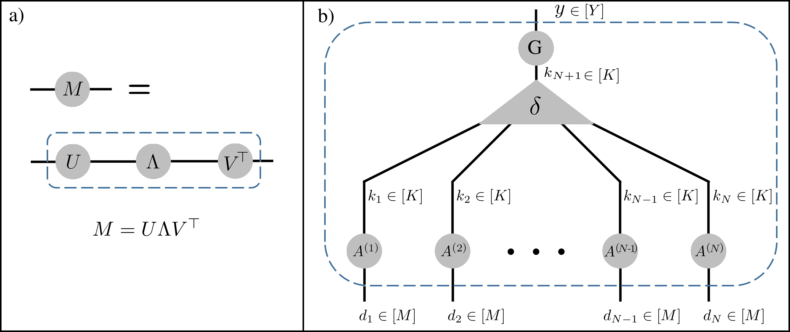
The role of the $\delta$ tensor in eq. 14 can be observed as ‘forcing’ the $k^{th}$ row of any matrix $A^{(j)}$ to be multiplied only by $k^{th}$ rows of the other matrices which in effect enforces same channel pooling⁶⁶ 6 If one were to switch the $\delta_{k_{1}...k_{N}}$ in eq. 14 by a general tensor ${\mathcal{G}}_{k_{1}...k_{N}}\in{\mathbb{R}}^{K\times\cdots\times K}$, a TN equivalent of an additional acclaimed decomposition would be attained, namely the Tucker decomposition. Similar to other tensor decompositions, the Tucker decomposition is more commonly given in an outer product form: ${\mathcal{A}}=\sum_{k_{1},...,k_{N}=1}^{K}{\mathcal{G}}_{k_{1}...k_{N}}{\mathbf{a}}^{k_{1},1}\otimes\cdots\otimes{\mathbf{a}}^{k_{N},N}$. .

We describe below a TN corresponding to the deep ConvAC calculation, which is presented in eq. 12. The ConvAC calculation is constructed as an inner-product between two tensors: ${\mathcal{A}}^{y}_{d_{1}...d_{N}}$ holding the weights of the network and ${\mathcal{A}}_{d_{1}...d_{N}}^{\textrm{(rank 1)}}({\mathbf{x}}_{1},\ldots,{\mathbf{x}}_{N})$ which is a rank-$1$ tensor holding the $N\cdot M$ values of the representation layer ($M$ representation functions applied on $N$ input patches).

Fig. 5 displays in full the TN for an $N=8$ ConvAC calculation. The upper block separated by a dashed line is the TN representing ${\mathcal{A}}_{d_{1}...d_{8}}$ whereas the lower block represents the rank-$1$ inputs tensor. Considering the upper block, it is worth noting that it is not a sketch of a TN but the actual full description complaint with the graph notations described in sec. 5.1. Accordingly, the two legged nodes represent matrices, where each matrix $A^{(l,j)}\in{\mathbb{R}}^{r_{l}\times r_{l-1}}$ (with $r_{-1}:=M$) is constructed such that it holds the convolutional weight vector ${\mathbf{a}}^{l,j,\gamma}\in{\mathbb{R}}^{r_{l-1}},\gamma\in[r_{l}]$ in its $\gamma^{th}$ row. The triangle node appearing between levels $l-1$ and $l$ represents an order $3$ tensor $\delta\in{\mathbb{R}}^{r_{l-1}\times r_{l-1}\times r_{l-1}}$, obeying eq. 13. The $\delta$ tensor is the element which dictates the same channel pooling in this TN construction.

As mentioned above, the lower block in fig. 5 is the TN representing ${\mathcal{A}}_{d_{1}...d_{8}}^{\textrm{(rank 1)}}({\mathbf{x}}_{1},\ldots,{\mathbf{x}}_{8})$. This simple TN is merely a single outer product of $N=8$ vectors ${\mathbf{v}}^{(0,j)}\in{\mathbb{R}}^{M},j\in[N]$ composing the representation layer presented in sec. 2.2, holding the values $v^{(0,j)}_{d_{j}}=f_{\theta_{d_{j}}}({\mathbf{x}}_{j})$. In compliance with the analogy between the function realized by the ConvAC and the projection of a many-body wave function onto a product state shown in eq. 8, the form ${\mathcal{A}}_{d_{1}...d_{8}}^{\textrm{(rank 1)}}$ assumes is exactly the form the coefficients tensor of a product state assumes when represented as a TN. As can be seen in fig. 5, a final contraction of the indices $d_{1},...,d_{8}$ results in the class scores vector calculated by the ConvAC, ${\mathbf{h}}_{y}({\mathbf{x}}_{1},...,{\mathbf{x}}_{8})$.

In appendix A, we present a recursive definition for the TN representing the a deep ConvAC of a general size (s.t. ${\textrm{log}}_{2}N\in{\mathbb{N}}$). As is demonstrated in appendix A, a contraction of a TN in an incremental fashion, starting with the input layer and moving up the network, exactly reproduces the computation preformed level-by-level along the network given in fig. 1. A generalization to a ConvAC with any pooling scheme is straightforward, where the size of the pooling window is translated into the number of edges incident to the $\delta$ tensors from below.

To conclude this section, we have presented a translation of the computation performed by a ConvAC to a TN. The convolutional weights are arranged as matrices (two legged nodes) placed along the network, and the same channel pooling characteristic is made available due to three legged $\delta$ tensors in a deep network, and an $N+1$ legged $\delta$ tensor in a shallow network. Finally, and most importantly for our upcoming analysis, the bond dimension of each level in the TN representing the ConvAC is equal to $r_{l}$, which is the number of feature maps (i.e. the number of channels) comprising that level in the corresponding ConvAC architecture. As we shall see in the following sections, this last equivalence will allow us to provide prescriptions regarding the number of channels in each level, when attempting to fit the correlations modeled by the network to the input correlations.

Convolutional networks, though often presented by graphical schemes that include nodes and edges which represent activation functions and weights, cannot be readily used as well-defined objects in graph theory. A general TN, on the other hand, is naturally represented by an underlying undirected graph describing its connectivity and a function that assigns a bond dimension to each edge. In this section we describe the TN we constructed in sec. 6.2 in graph-theoretic terminology.

The ability to represent a deep convolutional network (ConvAC) as a ‘legal’ graph, is a key accomplishment that the Tensor Networks tool brings forth. Our main results rely on this graph-theoretic description and tie the expressiveness of a ConvAC to a minimal cut in the graph characterizing it, via the connection to quantum entanglement measures. This is in fact a utilization of the ‘Quantum min-cut max-flow’ concept presented by Cui et al. (2016). Essentially, the quantum max-flow between $A$ and $B$ is a measure of the ability of the TN to model correlations between $A$ and $B$, and the quantum min-cut is a quantity that bounds this ability and can be directly inferred from the graph defining it — that of the corresponding TN.

As noted in sec. 6.2, the TN that describes the calculation of a ConvAC, i.e. a network that receives as inputs the $M$ representation channels and outputs $Y$ labels, is the result of an inner-product of two tensors ${\mathcal{A}}^{y}_{d_{1}...d_{N}}$ holding the weights of the network and ${\mathcal{A}}_{d_{1}...d_{N}}^{\textrm{(rank 1)}}({\mathbf{x}}_{1},\ldots,{\mathbf{x}}_{N})$ which is a rank-$1$ tensor holding the ‘input’ of $N$ vectors ${\mathbf{v}}^{(0,j)}\in{\mathbb{R}}^{M},j\in[N]$ composing the representation layer. In this section we focus on the TN that describes ${\mathcal{A}}^{y}_{d_{1}...d_{N}}$, which is the upper block of fig. 5 and is also reproduced as a stand-alone TN in fig. 6, referred to as the ‘ConvAC-weights TN’ and denoted by $\phi$. The TN $\phi$ has $N$ open edges with bond dimension $M$ that are to be contracted with the inputs ${\mathbf{v}}^{(0,j)}\in{\mathbb{R}}^{M},\ j\in[N]$ and one open edge with bond dimension $Y$ representing the values ${\mathcal{A}}^{y}_{d_{1}...d_{N}},\ y\in[Y]$ upon such a contraction, as is shown in fig 5.

To turn $\phi$ into a graph we do the following. First, we remove the open edge associated with the output. As our analysis is going to be based on flow between groups of input vertices, no flow can pass through that open edge therefore removing it does not influence our analysis. Second, we add $N$ virtual vertices incident to the open edges associated with the input. Those virtual vertices are the only vertices whose degree is equal to $1$ (see fig. 6). The TN $\phi$ is now described below using graph terminology:

• •

  An undirected graph $G(V,E)$, with a set of vertices $V$ and a set of edges $E$. The set of nodes is divided into two subsets $V=V^{\textrm{tn}}\mathbin{\mathaccent 0{\cdot}\cup}V^{\textrm{inputs}}$, where $V^{\textrm{inputs}}$ are the $N$ degree-$1$ virtual vertices and $V^{\textrm{tn}}$ corresponds to tensors of the TN.

• •

  A function $c~:~E\rightarrow{\mathbb{N}}$, associating a number $r\in{\mathbb{N}}$ with each edge in the graph, that equals to the bond dimension of the corresponding edge in the TN.

Having described the object representing the ConvAC-weights TN $\phi$, let us define an edge-cut set with respect to a partition of the $N$ nodes of $V^{\textrm{inputs}}$, and then introduce a cut weight associated with such a set. An edge-cut set with respect to the partition $V^{A}\mathbin{\mathaccent 0{\cdot}\cup}V^{B}=V^{\textrm{inputs}}$ is a set of edges $C$ s.t. there exists a partition $\tilde{V}^{A}\mathbin{\mathaccent 0{\cdot}\cup}\tilde{V}^{B}=V$ with $V^{A}\subset\tilde{V}^{A}~,~V^{B}\subset\tilde{V}^{B}$, and $C=\{(u,v)\in E:u\in\tilde{V}^{A},v\in\tilde{V}^{B}\}$. We note that this is a regular definition of an edge-cut set in a graph $G$ with respect to the partition of vertices $(V^{A},V^{B})$. Let $C=\{e_{1},...,e_{|C|}\}$ be such a set, we define its multiplicative cut weight as:

The weight definition given in eq. 15 is simply a multiplication of the bond dimensions of all the edges in a cut. Fig. 7 shows a pictorial demonstration of this weight definition, which is at the center of our results to come. In the following section, we use a max-flow / min-cut analysis on $\phi$ to obtain new results on the expressivity of the corresponding deep ConvAC via measures of entanglement w.r.t. a bi-partition of its input patches, and relate them to the number of channels in each layer of the ConvAC.

In claim 1 below, we provide an upper bound on the ability of a deep ConvAC to model correlations of its inputs, as measured by the Schmidt entanglement measure (see sec. 4.1). This claim is closely related to attributes of TNs that are known in different forms in the literature.

Claim 1 states that a measure of the ability of the TN $\phi$ (that models the ConvAC-weights) to represent correlations between two parts of its input, cannot be higher than the minimal weight over all the possible cuts in the network that separate between these two parts. Thus, if one wishes to construct a deep ConvAC that is expressive enough to model an intricate correlation structure according to some partition, it is advisable to verify that the convolutional network is able to support such correlations, by ensuring there is no cut separating these two parts in the corresponding TN that has a low weight. We will elaborate on such practical considerations in sec. 7.3.

The upper bound provided above, alerts us when a deep ConvAC is too weak to model a desired correlation structure, according to the number of channels in each layer. Below, we provide a lower bound similar in spirit to a bound shown in Cui et al. (2016). Their claim is applicable for a TN with general tensors (no $\delta$ tensors), and we adapt it to the ConvAC-weights TN (that has $\delta$ tensors) which in effect ensures us that the entanglement measure cannot fall below a certain value for any specific arrangement of channels per layer.

Theorem 2 above implies that the upper bound given in Claim 1 is saturated when all of the channel numbers in a deep ConvAC architecture are powers of some integer $p$. For a general arrangement of channel numbers, the upper bound is not tight and theorem 2 guarantees that the rank will not be lower than that of any ConvAC architecture with channel numbers which are powers of some integer $p$ yet are not higher than the original ConvAC channel numbers. Even though this is the lower bound we prove, we have a reason to believe the actual lower bound is much tighter. In appendix D, we show simulations which indicate that deviations from the upper bound are actually quite rare and unsubstantial in value.

When physicists choose a TN to represent the coefficients tensor of a certain wave function, the entanglement characterizing the wave function is taken into consideration, and a network which can best model it is chosen. Thus, understanding the correlations characteristics of the wave function serves as a prior knowledge that helps restrict the hypothesis space to a suitable TN architecture. In accordance with the analogies discussed above, we will draw inspiration from this approach in the analysis of our results from the previous section, as it represents a ‘healthy’ process of first quantifying the key correlations that the network is required to model, and then constructing it appropriately. This is in effect a control over the inductive bias of the network.

Accordingly, the bounds shown in the previous section not only provide us with theoretical observations regarding the role that the number of channels in each layer fulfils in the overall expressiveness of a deep ConvAC, but also entail practical implications for the construction of a deep network architecture when there is prior knowledge regarding the input. To get a feeling of what can be understood from the theoretical results, consider one-dimensional partitions similar in essence to the left-right partition and the interleaved partition depicted in fig 2. For a TN representing the ConvAC-weights with pooling windows of size $2$, $N$ input patches and $L={\textrm{log}}_{2}N$ layers (an $N=8$ example is shown in fig. 6), it is simple to see that the minimal weight of a cut with respect to the left-right partition obeys:

whereas the minimal weight of a cut w.r.t. the interleaved partition is guaranteed to be exponential in $N$ and obeys:

These are two examples that bring forth indications for the following ‘rule of thumb’. If one is interested in modeling elaborate correlations between pixels from opposite ends of an image, such as the ones characterizing face images for example, we see from the expression in eq. 16 that a small number of channels in deep layers can create an undesired ‘shortcut’ which harms the expressiveness of the network in a way that prevents it form modeling the required correlations. In this case, it is advisable to keep more parameters in the deeper layers in order to obtain a higher entanglement measure for the required partition. However, if one is interested in modeling only short ranged correlations, and knows that the typical input to the network will not exhibit relevant long ranged correlations, it is advisable to concentrate more parameters (in the form of more channels) in the lower levels, as it raises the entanglement measure w.r.t the partition which corresponds to short ranged correlations.

The two partitions analyzed above represent two extreme cases of the shortest and longest ranged correlations. However, the min-cut results shown in sec. 7.2 apply to any partition of the inputs, so that implications regarding the channel numbers can be drawn for any intermediate length-scale of correlations. The relevant layers that contribute to the min-cut between partitions $(A,B)$ for which both $A$ and $B$ have contiguous segments of a certain length $\xi$ can be pictorially identified, see for example fig. 8 for $\xi=3$. The minimal cut with respect to such a partition $(A,B)$ may only include the channel numbers $M,r_{0},...,r_{\left\lceil{{\textrm{log}}_{2}\xi}\right\rceil}$. This is in fact a generalization of the treatment above with $\xi=1$ for the interleaved partition and $\xi=N/2$ for the left-right partition. Any cut which includes edges in higher levels is guaranteed to have a higher weight than the minimal cut, as it will have to additionally include a cut of edges in the lower levels in order for a separation between $A$ and $B$ to actually take place. This can be understood by flow considerations in the graph underlying the TN — a cut that is located above a certain sub-branch can not assist in cutting the flow between $A$ and $B$ vertices that reside in that sub-branch.

For a data-set with features of a characteristic size $D$ (e.g. in a two-dimensional digit classification task it is the size of digits that are to be classified), such partitions of length scales $\xi<D$ are guaranteed to separate between different parts of a feature placed in any input location. However, in order to perform the classification task of this feature correctly, an elaborate function modeling a strong dependence between different parts of it must be realized by the network. As discussed above, this means that a high measure of entanglement with respect to this partition must be supported by the network, and now we are able to describe this measure of entanglement in terms of a min-cut in the TN graph. Concluding the above arguments, for a ConvAC with pooling windows of size $2$, if the characteristic features size is $D$ then the channel numbers up to layer $l=\left\lceil{{\textrm{log}}_{2}D}\right\rceil$ are more important than those of deeper layers. This understanding is verified and extended in section 8, where we present experiments exemplifying that the theoretical findings established above for the deep ConvAC, apply to a regular ConvNet architecture which involves the more common ReLU activations and average or max pooling. In natural images it may be hard to point out a single most important length scale $D$, however the conclusions presented in this section can be viewed as an incentive to better characterize the input correlations which are most relevant to the task at hand.

The exponential depth efficiency result shown in Cohen et al. (2016b), can be straightforwardly reproduced by similar graph-theoretic considerations. In appendix C, we show an upper bound on the rank of matricization of the convolutional weights tensor for a case of a general pooling window. The bound implies that any amount of edges in a cut that are connected to the same $\delta$ tensor will contribute their bond dimension only once to the multiplicative weight of this cut, thus effectively reducing the upper bound when many cut edges belong to the same $\delta$ tensor. This does not affect our analysis of the deep network above, as the $\delta$ tensors in that network are only three legged (see fig. 5). Therefore, a cut containing more than one $\delta$ tensor leg can be replaced by an equivalent cut containing only one leg of that $\delta$ tensor, and the value of $\min_{C}W_{C}$ is unchanged.

Observing fig.  4(b) which shows the TN corresponding to the shallow ConvAC architecture, the central positioning of a single $\delta$ tensor implies that under any partition of the inputs $(A,B)$, the minimal cut will obey $W_{C}^{\textrm{min}}={\textrm{min}}(M^{{\textrm{min}}(|A|,|B|)},k)$. Thus, in order to reach the exponential in $N$ measure of entanglement w.r.t. the interleaved partition that was obtained in eq. 17 for the deep network, the number of channels in the single hidden layer of the shallow network $k$, must grow exponentially with $N$. Therefore, one must exponentially enlarge the size of the shallow network in order to achieve the expressiveness that a polynomially sized deep network achieves, and an exponential depth efficiency is shown.

Overall, the conclusions regarding the architecture of a deep ConvAC drawn in this section are motivated by physical understandings of the role of correlations, and their connection to Tensor Networks. We have seen how the description of a deep ConvAC in terms of a valid graph enables the analysis of the effect that the number of channels in each of its layers has on the correlations it is able to model, through the tool of a minimal cut in the graph. In the following section, we demonstrate by experiments that the results and conclusions drawn above also hold in the more common setting of a ConvNet with ReLU activations and average or max pooling.

References

- Argyriou et al. [2005] Andreas Argyriou, Mark Herbster, and Massimiliano Pontil. Combining graph laplacians for semi-supervised learning. In NIPS, pages 67–74, 2005.
- Ballani et al. [2013] Jonas Ballani, Lars Grasedyck, and Melanie Kluge. Black box approximation of tensors in hierarchical tucker format. Linear algebra and its applications, 438(2):639–657, 2013.
- Bény [2013] Cédric Bény. Deep learning and the renormalization group. arXiv preprint arXiv:1301.3124, 2013.
- Blum and Mitchell [1998] Avrim Blum and Tom Mitchell. Combining labeled and unlabeled data with co-training. In Proceedings of the eleventh annual conference on Computational learning theory, pages 92–100. ACM, 1998.
- Blum et al. [2004] Avrim Blum, John Lafferty, Mugizi Robert Rwebangira, and Rajashekar Reddy. Semi-supervised learning using randomized mincuts. In Proceedings of the twenty-first international conference on Machine learning, page 13. ACM, 2004.
- Bruna et al. [2013] Joan Bruna, Wojciech Zaremba, Arthur Szlam, and Yann LeCun. Spectral networks and locally connected networks on graphs. arXiv preprint arXiv:1312.6203, 2013.
- Calegari et al. [2010] Danny Calegari, Michael Freedman, and Kevin Walker. Positivity of the universal pairing in 3 dimensions. Journal of the American Mathematical Society, 23(1):107–188, 2010.
- Carleo and Troyer [2017] Giuseppe Carleo and Matthias Troyer. Solving the quantum many-body problem with artificial neural networks. Science, 355(6325):602–606, 2017.
- Chen et al. [2017] Jing Chen, Song Cheng, Haidong Xie, Lei Wang, and Tao Xiang. On the equivalence of restricted boltzmann machines and tensor network states. arXiv preprint arXiv:1701.04831, 2017.
- Cohen and Shashua [2016] Nadav Cohen and Amnon Shashua. Convolutional rectifier networks as generalized tensor decompositions. International Conference on Machine Learning (ICML), 2016.
- Cohen and Shashua [2017] Nadav Cohen and Amnon Shashua. Inductive bias of deep convolutional networks through pooling geometry. In 5th International Conference on Learning Representations (ICLR), 2017.
- Cohen et al. [2016a] Nadav Cohen, Or Sharir, and Amnon Shashua. Deep simnets. IEEE Conference on Computer Vision and Pattern Recognition (CVPR), 2016a.
- Cohen et al. [2016b] Nadav Cohen, Or Sharir, and Amnon Shashua. On the expressive power of deep learning: A tensor analysis. Conference On Learning Theory (COLT), 2016b.
- Cui et al. [2016] Shawn X Cui, Michael H Freedman, Or Sattath, Richard Stong, and Greg Minton. Quantum max-flow/min-cut. Journal of Mathematical Physics, 57(6):062206, 2016.
- Dantzig and Fulkerson [1956] G Bv Dantzig and DR Fulkerson. On the min cut max flow theorem of networks. Annals of Mathematical Study, 38:215–222, 1956.
- Dasarathy et al. [2015] Gautam Dasarathy, Robert D Nowak, and Xiaojin Zhu. S2: An efficient graph based active learning algorithm with application to nonparametric classification. In COLT, pages 503–522, 2015.
- Deng et al. [2016] Dong-Ling Deng, Xiaopeng Li, and S Das Sarma. Exact machine learning topological states. arXiv preprint arXiv:1609.09060, 2016.
- Deng et al. [2017] Dong-Ling Deng, Xiaopeng Li, and S Das Sarma. Quantum entanglement in neural network states. arXiv preprint arXiv:1701.04844, 2017.
- Elias et al. [1956] Peter Elias, Amiel Feinstein, and Claude Shannon. A note on the maximum flow through a network. IRE Transactions on Information Theory, 2(4):117–119, 1956.
- Ford and Fulkerson [1956] Lester R Ford and Delbert R Fulkerson. Maximal flow through a network. Canadian journal of Mathematics, 8(3):399–404, 1956.
- Gu and Han [2012] Quanquan Gu and Jiawei Han. Towards active learning on graphs: An error bound minimization approach. In Data Mining (ICDM), 2012 IEEE 12th International Conference on, pages 882–887. IEEE, 2012.
- Guillory and Bilmes [2009] Andrew Guillory and Jeff A Bilmes. Label selection on graphs. In Advances in Neural Information Processing Systems, pages 691–699, 2009.
- Hackbusch [2012] Wolfgang Hackbusch. Tensor Spaces and Numerical Tensor Calculus, volume 42 of Springer Series in Computational Mathematics. Springer Science & Business Media, Berlin, Heidelberg, February 2012.
- Hall [2013] Brian C Hall. Quantum theory for mathematicians. Springer, 2013.
- He et al. [2015] Kaiming He, Xiangyu Zhang, Shaoqing Ren, and Jian Sun. Deep residual learning for image recognition. arXiv preprint arXiv:1512.03385, 2015.
- Henaff et al. [2015] Mikael Henaff, Joan Bruna, and Yann LeCun. Deep convolutional networks on graph-structured data. arXiv preprint arXiv:1506.05163, 2015.
- Huang and Wang [2017] Li Huang and Lei Wang. Accelerated monte carlo simulations with restricted boltzmann machines. Physical Review B, 95(3):035105, 2017.
- Janzamin et al. [2015] Majid Janzamin, Hanie Sedghi, and Anima Anandkumar. Beating the Perils of Non-Convexity: Guaranteed Training of Neural Networks using Tensor Methods. CoRR abs/1506.08473, 2015.
- Krizhevsky et al. [2012] Alex Krizhevsky, Ilya Sutskever, and Geoffrey E Hinton. ImageNet Classification with Deep Convolutional Neural Networks. Advances in Neural Information Processing Systems, pages 1106–1114, 2012.
- LeCun et al. [1998] Yann LeCun, Corinna Cortes, and Christopher JC Burges. The mnist database of handwritten digits, 1998.
- LeCun et al. [2015] Yann LeCun, Yoshua Bengio, and Geoffrey Hinton. Deep learning. Nature, 521(7553):436–444, May 2015.
- Lin and Tegmark [2016a] Henry W Lin and Max Tegmark. Critical behavior from deep dynamics: A hidden dimension in natural language. arXiv preprint arXiv:1606.06737, 2016a.
- Lin and Tegmark [2016b] Henry W Lin and Max Tegmark. Why does deep and cheap learning work so well? arXiv preprint arXiv:1608.08225, 2016b.
- Mehta and Schwab [2014] Pankaj Mehta and David J Schwab. An exact mapping between the variational renormalization group and deep learning. arXiv preprint arXiv:1410.3831, 2014.
- Menger [1927] Karl Menger. Zur allgemeinen kurventheorie. Fundamenta Mathematicae, 10(1):96–115, 1927.
- Niepert et al. [2016] Mathias Niepert, Mohamed Ahmed, and Konstantin Kutzkov. Learning convolutional neural networks for graphs. In Proceedings of the 33rd annual international conference on machine learning. ACM, 2016.
- Orús [2014] Román Orús. A practical introduction to tensor networks: Matrix product states and projected entangled pair states. Annals of Physics, 349:117–158, 2014.
- Oseledets [2011] Ivan V Oseledets. Tensor-train decomposition. SIAM Journal on Scientific Computing, 33(5):2295–2317, 2011.
- Oseledets and Tyrtyshnikov [2009] Ivan V Oseledets and Eugene E Tyrtyshnikov. Breaking the curse of dimensionality, or how to use svd in many dimensions. SIAM Journal on Scientific Computing, 31(5):3744–3759, 2009.
- Östlund and Rommer [1995] Stellan Östlund and Stefan Rommer. Thermodynamic limit of density matrix renormalization. Physical review letters, 75(19):3537, 1995.
- Pfeifer et al. [2014] Robert NC Pfeifer, Glen Evenbly, Sukhwinder Singh, and Guifre Vidal. Ncon: A tensor network contractor for matlab. arXiv preprint arXiv:1402.0939, 2014.
- Plenio and Virmani [2005] Martin B Plenio and Shashank Virmani. An introduction to entanglement measures. arXiv preprint quant-ph/0504163, 2005.
- Preskill [1998] John Preskill. Lecture notes for physics 229: Quantum information and computation. California Institute of Technology, 16, 1998.
- Sedghi and Anandkumar [2016] Hanie Sedghi and Anima Anandkumar. Training input-output recurrent neural networks through spectral methods. arXiv preprint arXiv:1603.00954, 2016.
- Sharir and Shashua [2017] Or Sharir and Amnon Shashua. On the expressive power of overlapping operations of deep networks. arXiv preprint arXiv:1703.02065, 2017.
- Sharir et al. [2016] Or Sharir, Ronen Tamari, Nadav Cohen, and Amnon Shashua. Tensorial mixture models. arXiv preprint arXiv:1610.04167, 2016.
- Simonyan and Zisserman [2014] Karen Simonyan and Andrew Zisserman. Very deep convolutional networks for large-scale image recognition. arXiv preprint arXiv:1409.1556, 2014.
- Stoudenmire and Schwab [2016] E Miles Stoudenmire and David J Schwab. Supervised learning with quantum-inspired tensor networks. arXiv preprint arXiv:1605.05775, 2016.
- Szegedy et al. [2015] Christian Szegedy, Wei Liu, Yangqing Jia, Pierre Sermanet, Scott Reed, Dragomir Anguelov, Dumitru Erhan, Vincent Vanhoucke, and Andrew Rabinovich. Going Deeper with Convolutions. CVPR, 2015.
- Szegedy et al. [2016] Christian Szegedy, Vincent Vanhoucke, Sergey Ioffe, Jon Shlens, and Zbigniew Wojna. Rethinking the inception architecture for computer vision. In Proceedings of the IEEE Conference on Computer Vision and Pattern Recognition, pages 2818–2826, 2016.
- Torlai and Melko [2016] Giacomo Torlai and Roger G Melko. Learning thermodynamics with boltzmann machines. Physical Review B, 94(16):165134, 2016.
- Verstraete and Cirac [2004] Frank Verstraete and J Ignacio Cirac. Renormalization algorithms for quantum-many body systems in two and higher dimensions. arXiv preprint cond-mat/0407066, 2004.
- Vidal [2007] Guifre Vidal. Entanglement renormalization. Physical review letters, 99(22):220405, 2007.
- Vidal [2008] Guifré Vidal. Class of quantum many-body states that can be efficiently simulated. Physical review letters, 101(11):110501, 2008.
- Vidal [2009] Guifre Vidal. Entanglement renormalization: an introduction. arXiv preprint arXiv:0912.1651, 2009.
- White [1992] Steven R White. Density matrix formulation for quantum renormalization groups. Physical review letters, 69(19):2863, 1992.
Appendix A A Recursive Construction of the Deep ConvAC Tensor Network
The calculation performed by a one-dimensional ConvAC for a general (s.t. ), is given by the recursively defined TN representation shown in fig. 11. is a vector of actual activations generated during a computation across in the level of the network shown in fig. 1. Recall that , and that is a vector in the representation layer (see fig. 5). To demonstrate that this TN indeed defines the calculations performed by a ConvAC, we conjecture that the equality in fig. 11 holds, namely that for the component of each such activations vector is given in terms of the vectors in the preceding layer by: