Long-range Interactions and Network Synchronization
Abstract.
The dynamical behavior of networked complex systems is shaped not only by the direct links among the units, but also by the long-range interactions occurring through the many existing paths connecting the network nodes. In this work, we study how synchronization dynamics is influenced by these long-range interactions, formulating a model of coupled oscillators that incorporates this type of interactions through the use of path Laplacian matrices. We study synchronizability of these networks by the analysis of the Laplacian spectra, both theoretically and numerically, for real-world networks and artificial models. Our analysis reveals that in all networks long-range interactions improve network synchronizability with an impact that depends on the original structure, for instance it is greater for graphs having a larger diameter. We also investigate the effects of edge removal in graphs with long-range interactions and, as a major result, find that the removal process becomes more critical, since also the long-range influence of the removed link disappears.
1. Introduction
The fact that most of complex systems are networked has made complex networks an important paradigm for studying such systems [51, 9, 20]. A complex network is a graph that represents the skeleton of such complex systems, ranging from biological and ecological to social and infrastructural ones. Representing such a variety of systems by a single mathematical object can be considered as a drastic simplification. However, complex networks have been very useful in explaining many properties of complex systems, which has been empirically validated their use for this purpose. In order to fill the gaps left by this simplified representation of complex systems a few extensions beyond the simple graph have been proposed. They include the use of hypergraphs, multiplexes and multilayer networks [16, 32], temporal graphs [29] and more recently the use of simplicial complexes [14, 22].
The previously mentioned extensions of complex systems representations try to ameliorate the emphasis paid by graphs on binary relations only. Then, in either of the previously developed representations of complex systems—hypergraphs, multiplexes, simplicial complexes—the binary relation is replaced by a unified -ary one, in which the individual is replaced by the group. Just to illustrate one example, in the hypergraph the binary relation between individuals is replaced by the -ary hyperedges in which nodes are assumed to be identical in their connectivity inside this group. Then, an important missing aspect of these representations is how to capture the influence of nodes in a network in a way that gradually decays with the separation of these nodes in the graph.
Recently, such approach has been proposed to account for long-range influences in a network by using extensions of the graph-theoretic concepts of adjacency and connectivity [23, 21]. In these works, a new paradigm is developed in which a node in a network is not only influenced by its nearest neighbours but by any other node in the graph. However, such influence is gradually tuned by the shortest path distance at which the influencers are from the influencee. It is obvious that this type of representation is not general for any kind of complex systems, as there are cases where such long-range influence does not exists. However, in the case of social systems such kind of long-range influence is certainly manifested in the so-called indirect peers pressure. Individuals in a social group are not only directly influenced by those connected to them but also by those socially close to them.
The approach proposed in [23, 21] is here applied to study how the long-range influences affect synchronization of the network nodes. In fact, when the units of a network are dynamical systems (for instance, periodic or chaotic oscillators), a collective phenomenon, characterized by the emergence of a common rhythm in all the units and observed in many natural and artificial systems, may emerge as the result of the interactions [61]. In this context it is known that the topology of the connections plays a fundamental role in determining the characteristics of the synchronous motion, its onset and stability [6]. Most of the works on the subject, however, consider interactions as only dictated by direct links, whereas, in this paper, we take into account influences through paths of length grater than one. Other studies [59, 42, 5, 36] have considered the case of oscillators embedded on a geometrical space and coupled with an intensity decaying with the geometric distance between them. In our paper, instead, the oscillators are viewed as the nodes of a network and the intensity of the interactions is weighted by considering the distance of the oscillators as measured by the length of the shortest path connecting them. This scenario has been modelled through the use of path Laplacian matrices, whose spectra are shown to determine the synchronizability of the system. In particular, we prove how increasingly weighting the long-range interactions always leads to the best scenario possible for synchronization and verify the result on network models and real-world structures. The quantitative impact of the long-range interactions depends on the network topology and on its specific properties such as the diameter, the density and the degree distribution. Finally, we study the effect of edge removal in networks with and without long-range interactions and, as a major finding, observe that it is more critical in the presence of such interactions, still exhibiting a higher synchronizability in this case than when the long-range interactions are not present.
2. Intuition and Mathematical formulation
In this section we formulate the general mathematical equations for considering long-range interactions (LRIs) in a system of coupled dynamical units. Let be a simple, undirected graph without self-loops having nodes and edges. Let us now write the equations of coupled dynamical units on a graph. Let us consider identical oscillators coupled with a coupling constant , where the oscillator has state variables . Then,
| (2.1) |
where represents the uncoupled dynamics, and the coupling function.
In matrix form Eqs. (2.1) can be written as follow
| (2.2) |
where , , indicates the identity matrix of order , and . The entries of the node-to-edges incidence matrix of the graph are defined as
| (2.3) |
We recall that the matrix is known as the Laplacian matrix of the graph and has entries
| (2.4) |
where is the degree of the node , the number of nodes adjacent to it. It is worth noting that the Laplacian matrix is related to the adjacency matrix of the graph via: , where is the diagonal matrix of degrees and the adjacency matrix has entries
| (2.5) |
Now, let us consider the following scenario of oscillators which are coupled according to a graph with a coupling strength . Consider that the oscillators can also couple in a weaker way if they are separated at a shortest path distance two. Let be the strength of the coupling between those oscillators, such that . In a similar way we can consider that oscillators at a given shortest path distance can couple together with a coupling strength which depends on their separation in the network. For instance, pairs of oscillators at distance three can couple with strength . This situation may well represents social scenarios as illustrated in Figure 2.1. In a social network, individuals are connected by certain social ties, such as friendship, collaboration, etc. Then, two individual directly connected to each other can influence each other in a relatively strong way. However, an individual in this network can also receive certain influence from others which are not directly connected to her. This influence is supposed to be smaller than the ones received from direct acquaintances, but not one that can be discarded at all. Let us consider a simple example of a scientific collaboration network. Two individuals are connected in this network if they have collaborated on a certain topic, e.g., they have published a paper together. It is clear that they have influenced each other in terms of their scientific styles. However, these two scientists are also influenced by individuals which are close to their topic of research although they have not collaborated together. This closeness is reflected in the fact that they are relatively close in this collaboration network in terms of shortest path distance. An individual from a completely different field is expected to be far from them in terms of the shortest path distance, and so to have a lower influence in their scientific styles.
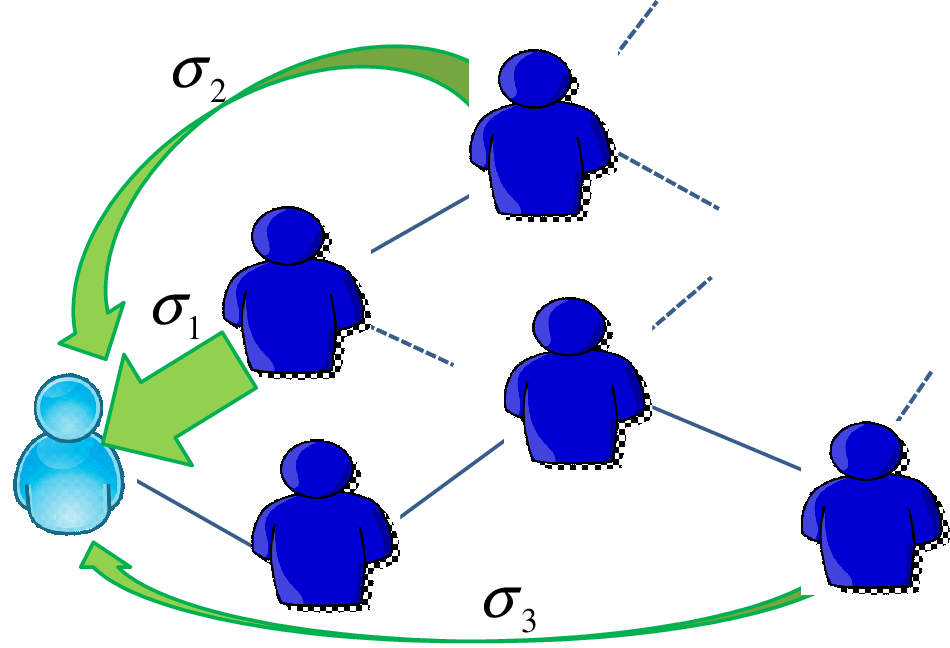
In mathematical terms this intuition can be formulated as follows. Let account for the strength of the cupling between pairs of oscillators separated by shortest path distances of one, two, and so forth up to the diameter of the graph, . Then, we can write
| (2.6) |
The simplest way to account for these long-range influences is by considering that the coupling strength between individuals decays as certain law of the shortest path distance. That is, if we consider a power-law decay of the strength of coupling with the distance we get, assuming that and that the rest are just a fraction of it,
| (2.7) |
Similarly, if we assume an exponential decay we obtain
| (2.8) |
We call these equations the Mellin and Laplace transforms, respectively, of the coupled dynamical units on a graph.
Let us now define the -path incidence matrices which account for these coupling of non-nearest-neighbours in the graph. Let denote a shortest path of length between and . The nodes and are called the endpoints of the path . Because there could be more than one shortest path of length between the nodes and we introduce the following concept. The irreducible set of shortest paths of length in the graph is the set in which the endpoints of every shortest path in the set are different. Every shortest path in this set is called an irreducible shortest path. Let be the graph diameter, i.e., the maximum shortest path distance in the graph.
Definition 1.
Let . The -path incidence matrix, denoted by , of a connected graph of nodes and irreducible shortest paths of length is defined as:
| (2.9) |
Obviously Let us now rewrite our Mellin and Laplace transformed equations, respectively, in matrix-vector form using the -path incidence matrix as follow
| (2.10) |
| (2.11) |
The parameters and account for the strength of the coupling of the oscillators at a given distance. The smallest the values of these parameters the stronger the coupling between the oscillators at a given distance. For instance when () there is a very weak influence of non-nearest neighbours and we recover the classical model in which there is no long-range coupling. When () the strength of the coupling between oscillators at any distance is the same, which corresponds to the situation of the classical model of coupled oscillators on a complete graph . Thus, in every case we always recover the original model of coupled oscillators on graphs for large values of the parameters in the transforms of the -path incidence matrices and we approach the coupling on a complete graph when these parameters tend to zero.
Note that in our approach the coupling strength depends on the shortest path distance. This differs from the notion of accessability matrix [35], which accounts for the existence of paths of arbitrary length between the nodes with unitary weights.
2.1. Example. Long-range interactions in the Kuramoto model
In this section we particularize the equations for the coupled system to the case of phase oscillators, so that to consider LRIs in the Kuramoto model [58]. Let us consider phase oscillators on graph coupled with an identical coupling constant , where the oscillator has phase and intrinsic frequency . Then,
| (2.12) |
or in matrix form
| (2.13) |
The consideration of LRIs in the way we have described previously will give rise to the following transforms of the Kuramoto model:
| (2.14) |
for the Mellin transform, and
| (2.15) |
for the Laplace transform. In matrix-vector form they are given by
| (2.16) |
for the Mellin transform, and
| (2.17) |
for the Laplace transform. Here again when () the coupling between oscillators at distance larger than one is almost zero and we recover the classical Kuramoto model where there is no LRIs. On the other hand, when () the strength of the coupling between oscillators at any distance is the same and we obtain the Kuramoto model on a complete graph .
3. Synchronizability and Laplacian Spectra
The Laplacian matrix of the graph is positive semi-definite with eigenvalues denoted by: . If the network is connected, the multiplicity of the zero eigenvalue is equal to one, i.e., , and the smallest nontrivial eigenvalue is known as the algebraic connectivity of the network. It is now well known that there are two types of networks with bounded and unbounded synchronization regions in the parameter space. One large class of dynamic networks have an unbounded synchronized region specified by
| (3.1) |
where constant depends only on the node dynamics, a bigger spectral gap implies a better network synchronizability, namely a smaller coupling strength is needed [12, 17, 18, 39].
Another large class of dynamic networks have a bounded synchronized region specified by
| (3.2) |
where constants depend only on the node dynamics as well, and a bigger eigenratio implies a better network synchronizability, which likewise means a smaller coupling strength is needed [54, 30].
Here we only consider the latter criterion while the former can be discussed similarly. As introduced, in this scenario the synchronizability of the graph depends on the eigenratio of the second smallest and the largest eigenvalues of the Laplacian matrix:
| (3.3) |
Now, we have generalized the Laplacian matrix to the so-called -path Laplacian matrices which are defined as follow.
Definition 2.
Let . The -path Laplacian matrix, denoted by , of a connected graph of nodes is defined as:
| (3.4) |
where is the number of irreducible shortest paths of length that are originated at node , i.e., its -path degree. It is straightforward to realize that in a similar way as it happens for the graph Laplacian.
We now extend the notion of a connected component of a graph to the -connected component.
Definition 3.
Let be a simple graph and let . A -connected component of is a subgraph , , , such that for all there is a shortest path of length . If the -connected component includes all the vertices and edges of , the graph is said to be -connected.
The following is an important property of the -path Laplacian matrix proved by Estrada in 2012 [19].
Theorem 4.
Let be a simple graph and let . The matrix is positive semidefinite. Moreover, the multiplicity of the zero eigenvalue of is equal to the number of -connected components of the graph.
The previous result has an important implication for the study of synchronization on graphs using the -path Laplacian matrix. Although a graph can be connected in the usual way—here it should be said 1-connected—it not necessarily should be -connected. Then, a synchronization process taking place between agents separated at distance in that graph may not give rise to a unique synchronized state. For instance, a synchronization process taking place on the pairs of nodes separated at distance 2 in the pentagon gives rise to a unique synchronized state because the graph is -connected, but a similar process on the hexagon conduces to two synchronized states because there are two -connected components in this graph. Then, the use of the Mellin and Laplace transformed dynamical systems, like the ones introduced in this work, require a transformation of the -path Laplacian matrices such that they account for the decay of the influence of oscillators separated at different distances in the graph. Then, we have the following.
Definition 5.
Let be a simple connected graph and let . The Mellin and Laplace transformed -path Laplacian matrices of are given by
| (3.5) |
Now, we can interpret the LRI-model in the following way. Consider a simple connected graph and the following transformation: , such that and is a surjective mapping that assigns a weight to each of the elements of . The weights are given by the Mellin or Laplace transforms and they are specific for each graph, that is or for , and for connected pairs of nodes. The main consequence of this is that we can generalize the synchronizability definition (3.3) to:
| (3.6) |
where and are the largest and second smallest eigenvalues of the transformed -path Laplacian matrices. The most important consequence of this new formulation is that when the weighted graph tends to the original graph . In addition, when the weighted graph tends to the complete graph with nodes, . It is known that the Laplacian eigenvalues of are all equal to but one which is equal to zero. Then, the following result holds.
Lemma 6.
Let and let be the Mellin or Laplace transformed -path Laplacian of the graph. Then, we have the following behavior of the generalized eigenratio
| (3.7) |
Similarly, for networks of dynamical units with unbounded synchronized region, if one considers synchronizability as measured by the smallest non-zero eigenvalue of the -path Laplacian normalized by the number of nodes, i.e., , the following lemma holds.
Lemma 7.
Let and let be the Mellin or Laplace transformed -path Laplacian of the graph. Then, we have the following behavior of the normalized smallest eigenvalue
| (3.8) |
In addition, the following Lemma characterizes the behavior of the smallest non-zero eigenvalue and of the largest eigenvalue of the transformed -path Laplacian with respect to the transform parameter ( for the Mellin transform or for the Laplace transform).
Lemma 8.
Let be a simple graph and let be the transformed -path Laplacian of with parameter where (Mellin) and for (Laplace). Let be the largest eigenvalue of . Then, if (Mellin) or (Laplace) we have that and . That is, and are non-increasing with or
Proof.
Let be a nontrivial vector. Using the Rayleigh-Ritz theorem we have that
and
Let us select a normalized vector for the sake of simplicity. Then,
| (3.9) |
| (3.10) |
Then, for a fixed vector , a decrease of the parameter i.e., increase of the parameters or , makes that and decay or remain at their previous value, so in general they are non-increasing with or . ∎
Based on these considerations and on the fact that , one could expect that is also increasing on average when or are decreasing. Numerical results, which are shown in the next section, along with the fitting functions, show that, in addition, the decay is monotonic. This implies that for any network of coupled oscillators, independently of its topology and the unit dynamics, the increase of the long-range coupling between oscillators, i.e., , produces the best possible synchronizability.
We illustrate this result by calculating and for Erdős-Renyi (ER) random graphs with and for increasing values of the parameters and of the -path Laplacian matrices. Fig. 3.1 clearly shows that for the best possible synchronizability is obtained, whereas for the synchronizability of the original graph is recovered.


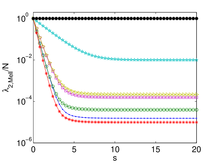
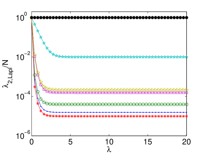
A note of caution should be written here. The fact that for the network behaves like a complete graph does not mean that the current results are trivial in the sense that we replace the graph under study by a complete graph. If we consider values of close but not exactly equal to zero, the synchronizability of the networks approach the best possible value, but (and this is an important but) it still depends on the topology of the network. In order to illustrate this fact we investigate next how the values of and change with or for a few different types of graphs. In particular, we have done the calculations for a series of graphs: the star topology, the triangular and square lattices, the ring, the Barbell graph and the path graph. For each of these graphs we have applied the Mellin and the Laplace transform and computed the synchronizability measures for different values of or . The results, shown in Fig. 3.2, include as reference the synchronizability of the complete graph, which clearly does not depend on the transform parameters. The curves clearly show that the synchronizability tends to one for all the graphs as LRIs are increasingly weighted (), but the impact of LRIs is a function of the graph topology.


To further corroborate our finding, we considered a dataset of 54 real-world networks (see Appendix for descriptions of the networks) and calculated and without and with LRIs. Fig. 3.3(a) shows the results of the change of —the results for are very similar—with the parameter of the Mellin transform. This confirms our previous result that the rate of change of the spectral ratio with the parameters of the transforms used in the synchronization models depends on the topology of the network. Just to give a clear example of the meaning of this finding, when there are networks (such as SoftwareMysql, network 17 of Table 1 in Appendix) for which the relative value of is approximately 30% of the best possible value while for others (such as Skipwith, network 29 of Table 1 in Appendix) it approaches 60%. This demonstrates that the topology of the network continues to play a fundamental role in the synchronizability of the system even when the long-range influence of the nodes is very high. Knowing how the network topology influences the rate of change of the spectral parameters and consequently of their synchronizability is an important open question that should be further investigated. Some insights on this is provided by the following considerations on how to fit the data of Fig. 3.3(a). To illustrate this, let us first consider the star topology. For this network we have been able to find a closed formula for the eigenvalues of the -path transformed Laplacian matrix. Let , , and indicate the -th eigenvalue of the original Laplacian matrix, of the -path transformed Laplacian matrix (here, for simplicity we consider only the Mellin transform, but similar results hold for the Laplace one) and of the Laplacian matrix of the complete graph. For the star topology, we have:
| (3.11) |
with (this expression has been analytically checked up to and numerically verified for larger ).
We have then generalized this formula for an arbitrary network as follows:
| (3.12) |
where now is a fitting parameter (one for each eigenvalue to fit) that depends on the topology we are investigating. Note that for we have and for we have (the eigenvalues of the original network).
Finally we propose to fit as:
| (3.13) |
An example for three real-world networks is shown in Fig. 3.3(b). This fitting provides an approximate formula describing how changes with . Noticeably, the formula depends on the characteristics of the topology through the eigenvalues and of the original network Laplacian and some fitting parameters and .


In the case of the Kuramoto model we show some further results confirming the beneficial effect of LRIs. For this model, in fact, it is known that plays a fundamental role. In particular, for identical oscillators, it is known that the synchronization time scales with the inverse of . Based on this and on the result of Lemma 7, we thus expect that LRIs in the Kuramoto model promote synchronization. For the numerical simulations, we considered two different network topologies, ER and scale-free (SF) random graphs [4], and monitored synchronization by measuring the order parameter , defined as
| (3.14) |
where is a sufficiently large averaging window. Values of close to one indicates a high degree of synchronization, while low values (close to zero) the absence of coherence among the oscillators. Fig. 3.4(a) shows the behavior of the order parameter vs. the coupling for an ER network with and different values of . As expected, decreasing favors synchronization. Similar results are obtained for SF networks (Fig. 3.4(b)). The results are illustrated for Mellin transformed -path Laplacian matrices, but also hold when the Laplace transform is considered.


4. How does network topology influence the role of LRIs?
The analysis of the effects of LRIs on the synchronizability of real-world networks has revealed that the quantitative impact of LRIs varies from network to network. In this section we study how the effects of LRIs on synchronizability depend on some network characteristics by considering a series of artificial networks with controlled attributes.
To begin, we start investigating how the effects of LRIs depend on network diameter. To this aim, we have considered the Watts-Strogatz model generating small-world networks through a rewiring process applied to a pristine regular graph [65]. More specifically, we started from a ring with 4-nearest neighbors and then rewired the links with a progressively increasing rewiring probability, labeled as . This produces networks with the same number of nodes and links, but with a different diameter (large for , small for ). Figs. 4.1(a) and (d) illustrate the results. LRIs always lead to enhancement of synchronizability, but the larger is the diameter the larger are the (beneficial) effects of LRIs.
We have then studied how the effects of LRIs are influenced by the average degree . To this aim, we have considered networks with the same number of nodes and a growing number of links. The ER model is adopted. Figs. 4.1(b) and (e) shows that the smaller is the average degree the larger are the effects of LRIs on synchronizability, so that we conclude that LRIs are more important in networks with smaller degree.
Finally, we have investigated the effect of degree heterogeneity by simulating networks with the same number of nodes, number of links and diameter, but different degree distributions. These are obtained by using the network model described in [28], which parameterizes with the tuning from one network type to the other ( corresponds to a SF network, while to an ER network). Fig. 4.1(c) and (f) shows that the effects on poorly depend on the topology, but those on the ratio are much more important on SF networks rather than in ER structures. So, SF networks receive more benefits from the inclusion of LRIs.


5. Critical edges for synchronization
To further study the interplay between synchronizablity and structure, in this section we investigate the effect of the edge removal on synchronization in the absence and in the presence of LRIs. More specifically, edge removal is performed according to different strategies; we consider either the removal of links chosen at random or according to some criterion ranking the edges. Since synchronization occurs through the exchange, among the network nodes, of the information on their dynamical state, those links in which information traffic is larger should be considered as the most critical. To account for this, we considered different measures of edge centrality.
The first one is edge degree calculated as , where and are the node degrees of and . The larger is the edge degree the more critical is the edge, so first we remove edges with larger edge degree.
Edge degree, however, only considers one-hop information exchanges, whereas information in a network is transmitted through the many existing paths from node to node. If one limits to consider shortest paths, edge centrality can be measured by edge betweeness centrality (EBC) defined as
| (5.1) |
where is the number of shortest paths from node to passing through and the total number of shortest paths between nodes and . The larger is the value of the EBC, the more critical is the edge and so has to be removed first.
If information is assumed to flow not only through shortest paths, then one can takes into account two other measures of edge centrality as recently introduced in [24]: the communicability function and the communicability angle. The first is defined as
| (5.2) |
The communicability function is calculated for the network edges, that is, where , providing a measure to rank them: the smaller is the poorer is the communicability between and , so the more critical is the edge. Therefore, if one wants to remove the critical edges according to this measure, those edges with small values of should be removed first.
Finally, the communicability angle is defined as
| (5.3) |
Restricting the analysis to the network edges, one has where . The larger is the poorer is the communicability between and , so the more critical is the edge. Edges with high values of should be then removed first.
Given a graph , for each of the edge centralities considered, we have ranked the edges in decreasing order and removed a percentage of those that do not disconnect the graph, creating a graph with the same nodes of and edges . We have then compared the synchronization measures ( and ) for network and that of the original network . We have then considered LRIs in both and and again compared the synchronization measures for these graphs. The analysis has been performed for each of the 54 real-world networks of the dataset.
Fig. 5.1 shows how the synchronizability of real-world networks, measured by the normalized parameters (Fig. 5.1(a)-(c)) and (Fig. 5.1(d)-(f)), is affected by LRIs (here, and indicate the values of and for the network after removing the edges). To facilitate the visualization, the networks have been ordered according to the descending values of , where the removal of the links has been done according to decreasing values of the communicability angle.
We observe that the edge removal affects more significantly synchronization in graphs with LRI than in the no-LRI scheme due to the fact that, when a “physical” link is removed, then also its long-range influence is removed. Synchronizability of the network without the removed edges is still larger if LRIs are allowed than if it is not, which means that the system can work better after the edge removal if such long-range interactions are present than if not. Finally, comparing the different edge removal methods, we notice that edge degree does not identify important edges, as the removal by this index leaves the networks almost unaffected in terms of the synchronizability. On the contrary, it seems that the best identifiers of critical edges are those accounting for effects going beyond nearest neighbors interactions, that is, the edge betweenness (shortest paths) and the communicability angle (all walks), because the removal by them affected the most the synchronizability.


6. Conclusions
In this work we have studied the impact of long-range interactions (LRIs) on synchronization. To account for LRIs, oscillators are coupled through path Laplacian matrices into a model that generalizes the traditional one, based on the classical Laplacian of a graph, and includes it as a special case for . As network synchronizability is essentially determined by the spectra of the Laplacian, and in particular by the smallest non-zero eigenvalue or by the ratio between the smallest non-zero eigenvalue and the largest one, we have thus studied these quantities for the graphs with LRIs.
Our theoretical considerations led to the conclusion that, increasing the weight of LRIs, any network of coupled oscillators, independently of the topology and the dynamics of the units, approaches the best possible scenario for synchronization. The specific path towards this limit condition depends on the network properties. We have performed numerical simulations both on real-world examples and on network models, and found results in perfect agreement with the theoretical expectations.
A significant result is the dependence of the impact of LRIs on some topological properties of interest, such as the diameter, the density and the degree distribution. We have found that a larger diameter, a smaller average degree or a higher heterogeneity in the degree distribution are all factors contributing to increase the positive impact of LRIs on synchronizability with respect to the scenario without LRIs.
Finally, we have studied the effects of the removal of critical edges in the absence and in the presence of LRIs, where criticality has been measured according to different topological measures of edge centrality. This analysis, carried out on real-world networks of different sizes and characteristics, points out scenarios common to all the examples considered. First of all, we have found that edge removal has a larger impact on the synchronizability of networks with LRIs rather than on the structures without LRIs. This is due to the fact that, when a physical link is removed, then also the long-range interactions it allowed are affected. However, synchronizability of the networks without the removed edges is still larger if LRIs are allowed than if not, confirming the general result that the presence of long-range interactions always favors synchronizability. Finally, we have observed that the most critical edges for synchronization are those having high values of the edge betweenness or of the communicability angles, i.e., are ranked according to measures taking into account effects going beyond nearest neighbors interactions.
The current approach can be extended to directed graphs. The first step in doing so is to generalize the -path Laplacian matrices for such graphs. In this case there are two kinds of -path Laplacians, namely the in- and the out-degree -path Laplacians. That is, we should first generalize the in- and out-degrees to account for the indirect influence of nodes. The generalization is, however, straightforward. We only need to consider the number of directed shortest paths of length from the node to any other node in the graph to account for the out--degree of the node . Similarly, we can define the in--degree of the node by taking the number of directed shortest paths of length from any node in the graph to the node . For the synchronization dynamics we should consider the out-degree -path Laplacians in a similar way as we have done in the current work for the undirected graphs. For directed graphs synchronizability has to be checked in the complex plane as the Laplacian eigenvalues are in general complex. However, provided that the graph is strongly connected, the generalization of -path Laplacian matrix accounting for oriented paths still yields for () a complete graph, thus favoring synchronizability. The mathematical properties of these in- and the out-degree -path Laplacians are not trivial and deserve to be considered in a separate work.
Appendix A Real-world network dataset
The real-world networks used in this paper belong to different domains: ecological (includes food webs and ecosystems), social (networks of friendships, communication networks, corporate relationships), technological (internet, transport, software development networks), informational (vocabulary networks, citations) and biological (protein-protein interaction networks, transcriptional regulation networks). The dataset comprises networks of different sizes, ranging from to nodes. The networks are listed in Table 1.
| No. | Dataset | Domain | N | m | Ref. | |
|---|---|---|---|---|---|---|
| 1 | ReefSmall | ecological | 50 | 524 | 0.9904 | [53] |
| 2 | StMartin | ecological | 44 | 218 | 0.6589 | [43] |
| 3 | Internet-1998 | technological | 3522 | 6324 | 0.6503 | [25] |
| 4 | Trans-urchin | biological | 45 | 80 | 0.5974 | [47] |
| 5 | KSHV | biological | 50 | 122 | 0.5143 | [63] |
| 6 | ODLIS | informational | 2898 | 16381 | 0.4696 | [2] |
| 7 | Software Abi | technological | 1035 | 1736 | 0.4036 | [50] |
| 8 | Internet-1997 | technological | 3015 | 5156 | 0.3488 | [25] |
| 9 | USA Air 97 | technological | 332 | 2126 | 0.3095 | [2] |
| 10 | Sawmill | social | 36 | 62 | 0.2802 | [46] |
| 11 | Grassland | ecological | 75 | 113 | 0.2789 | [44] |
| 12 | World-trade | informational | 80 | 875 | 0.2726 | [8] |
| 13 | Trans-Ecoli | biological | 328 | 456 | 0.2715 | [47] |
| 14 | Neurons | biological | 280 | 1973 | 0.2122 | [66] |
| 15 | Ythan1 | ecological | 134 | 597 | 0.2102 | [31] |
| 16 | Hpyroli | biological | 710 | 1396 | 0.1978 | [37] |
| 17 | Software Mysql | technological | 1480 | 4221 | 0.1850 | [50] |
| 18 | YeastS | biological | 2224 | 7049 | 0.1736 | [10] |
| 19 | Geom | social | 3621 | 9461 | 0.1666 | [8] |
| 20 | Chesapeake | ecological | 33 | 72 | 0.1664 | [13] |
| 21 | Benguela | ecological | 29 | 191 | 0.1490 | [67] |
| 22 | Software Digital | technological | 150 | 198 | 0.1470 | [50] |
| 23 | Hi-tech | social | 33 | 91 | 0.1420 | [33] |
| 24 | Zackar | social | 34 | 78 | 0.1375 | [69] |
| 25 | PRISON-Sym | social | 67 | 142 | 0.1309 | [41] |
| 26 | ScotchBroom | ecological | 154 | 370 | 0.1269 | [45] |
| 27 | PIN Ecoli | biological | 230 | 695 | 0.1231 | [11] |
| 28 | Roget | informational | 994 | 3641 | 0.1171 | [3] |
| 29 | Skipwith | ecological | 35 | 364 | 0.1098 | [68] |
| 30 | StMarks | ecological | 48 | 221 | 0.1011 | [27] |
| 31 | social3 | social | 32 | 80 | 0.1002 | [70] |
| 32 | Malaria PIN | biological | 229 | 604 | 0.0999 | [34] |
| 33 | Canton | ecological | 108 | 708 | 0.0943 | [62] |
| 34 | Drugs | social | 616 | 2012 | 0.0917 | [1] |
| 35 | BridgeBrook | ecological | 75 | 547 | 0.0896 | [55] |
| 36 | Stony | ecological | 112 | 832 | 0.0844 | [7] |
| 37 | Dolphins | social | 62 | 159 | 0.0826 | [40] |
| 38 | ElVerde | ecological | 156 | 1441 | 0.0813 | [57] |
| 39 | PIN Human | biological | 2783 | 6438 | 0.0733 | [60] |
| 40 | electronic2 | technological | 252 | 399 | 0.0730 | [48] |
| 41 | Software-VTK | technological | 771 | 1369 | 0.0717 | [50] |
| 42 | Transc-yeast | biological | 662 | 1062 | 0.0668 | [47] |
| 43 | CorporatePeople | social | 1586 | 13126 | 0.0654 | [15] |
| 44 | electronic3 | technological | 512 | 819 | 0.0595 | [48] |
| 45 | Software-XMMS | technological | 971 | 1809 | 0.0471 | [50] |
| 46 | electronic1 | technological | 122 | 189 | 0.0463 | [48] |
| 47 | SmallW | informational | 233 | 994 | 0.0422 | [2] |
| 48 | Shelf | ecological | 81 | 1476 | 0.0356 | [38] |
| 49 | Coachella | ecological | 30 | 261 | 0.0300 | [64] |
| 50 | Power grid | technological | 4941 | 6594 | 0.0067 | [65] |
| 51 | ColoSPG | social | 324 | 347 | [56] | |
| 52 | Drosophila PIN | biological | 3039 | 3715 | [26] | |
| 53 | Pin- Bsubtilis | biological | 84 | 98 | [52] | |
| 54 | PIN-Afulgidus | biological | 32 | 38 | [49] |
References
- [1] Data for this project were provided, in part, by NIH grants DA12831 and HD41877, 2001.
- [2] Pajek datasets, 2001.
- [3] Roget’s thesaurus of english words and phrases, project gutenberg, 2002.
- [4] Réka Albert, Hawoong Jeong, and Albert-László Barabási. Error and attack tolerance of complex networks. nature, 406(6794):378–382, 2000.
- [5] Celia Anteneodo, Sandro E de S Pinto, Antônio M Batista, and Ricardo L Viana. Analytical results for coupled-map lattices with long-range interactions. Physical Review E, 68(4):045202, 2003.
- [6] Alex Arenas, Albert Díaz-Guilera, Jurgen Kurths, Yamir Moreno, and Changsong Zhou. Synchronization in complex networks. Physics Reports, 469(3):93–153, 2008.
- [7] Daniel Baird and Robert E Ulanowicz. The seasonal dynamics of the chesapeake bay ecosystem. Ecological monographs, 59(4):329–364, 1989.
- [8] Vladimir Batagelj and Andrej Mrvar. Analysis of large networks. 2006.
- [9] Stefano Boccaletti, Vito Latora, Yamir Moreno, Martin Chavez, and D-U Hwang. Complex networks: Structure and dynamics. Physics reports, 424(4):175–308, 2006.
- [10] Dongbo Bu, Yi Zhao, Lun Cai, Hong Xue, Xiaopeng Zhu, Hongchao Lu, Jingfen Zhang, Shiwei Sun, Lunjiang Ling, Nan Zhang, et al. Topological structure analysis of the protein–protein interaction network in budding yeast. Nucleic acids research, 31(9):2443–2450, 2003.
- [11] Gareth Butland, José Manuel Peregrín-Alvarez, Joyce Li, Wehong Yang, Xiaochun Yang, Veronica Canadien, Andrei Starostine, Dawn Richards, Bryan Beattie, Nevan Krogan, et al. Interaction network containing conserved and essential protein complexes in escherichia coli. Nature, 433(7025):531–537, 2005.
- [12] Guanrong Chen and Zhisheng Duan. Network synchronizability analysis: A graph-theoretic approach. Chaos: An Interdisciplinary Journal of Nonlinear Science, 18(3):037102, 2008.
- [13] Robert R Christian and Joseph J Luczkovich. Organizing and understanding a winter’s seagrass foodweb network through effective trophic levels. Ecological modelling, 117(1):99–124, 1999.
- [14] Owen T Courtney and Ginestra Bianconi. Generalized network structures: The configuration model and the canonical ensemble of simplicial complexes. Physical Review E, 93(6):062311, 2016.
- [15] Gerald F Davis, Mina Yoo, and Wayne E Baker. The small world of the american corporate elite, 1982-2001. Strategic organization, 1(3):301–326, 2003.
- [16] Manlio De Domenico, Albert Solé-Ribalta, Emanuele Cozzo, Mikko Kivelä, Yamir Moreno, Mason A Porter, Sergio Gómez, and Alex Arenas. Mathematical formulation of multilayer networks. Physical Review X, 3(4):041022, 2013.
- [17] Zhisheng Duan, Guanrong Chen, and Lin Huang. Complex network synchronizability: Analysis and control. Physical Review E, 76(5):056103, 2007.
- [18] Zhisheng Duan, Chao Liu, and Guanrong Chen. Network synchronizability analysis: The theory of subgraphs and complementary graphs. Physica D: Nonlinear Phenomena, 237(7):1006–1012, 2008.
- [19] Ernesto Estrada. Path laplacian matrices: introduction and application to the analysis of consensus in networks. Linear Algebra and its Applications, 436(9):3373–3391, 2012.
- [20] Ernesto Estrada. The structure of complex networks: theory and applications. Oxford University Press, 2012.
- [21] Ernesto Estrada, Ehsan Hameed, Naomichi Hatano, and Matthias Langer. Path laplacian operators and superdiffusive processes on graphs. i. one-dimensional case. Linear Algebra and its Applications, 523:307–334, 2017.
- [22] Ernesto Estrada and Grant Ross. Centralities in simplicial complexes. arXiv preprint arXiv:1703.03641, 2017.
- [23] Ernesto Estrada and Eusebio Vargas-Estrada. How peer pressure shapes consensus, leadership, and innovations in social groups. Scientific Reports, 2013.
- [24] Ernesto Estrada, Eusebio Vargas-Estrada, and Hiroyasu Ando. Communicability angles reveal critical edges for network consensus dynamics. Physical Review E, 92(5):052809, 2015.
- [25] Michalis Faloutsos, Petros Faloutsos, and Christos Faloutsos. On power-law relationships of the internet topology. In ACM SIGCOMM computer communication review, volume 29, pages 251–262. ACM, 1999.
- [26] Loic Giot, Joel S Bader, C Brouwer, Amitabha Chaudhuri, Bing Kuang, Y Li, YL Hao, CE Ooi, Brian Godwin, E Vitols, et al. A protein interaction map of drosophila melanogaster. science, 302(5651):1727–1736, 2003.
- [27] Lloyd Goldwasser and Jonathan Roughgarden. Construction and analysis of a large caribbean food web. Ecology, 74(4):1216–1233, 1993.
- [28] Jesús Gómez-Gardeñes and Yamir Moreno. From scale-free to erdos-rényi networks. Physical Review E, 73(5):056124, 2006.
- [29] Petter Holme and Jari Saramäki. Temporal networks. Physics reports, 519(3):97–125, 2012.
- [30] Liang Huang, Qingfei Chen, Ying-Cheng Lai, and Louis M Pecora. Generic behavior of master-stability functions in coupled nonlinear dynamical systems. Physical Review E, 80(3):036204, 2009.
- [31] M Huxham, S Beaney, and D Raffaelli. Do parasites reduce the chances of triangulation in a real food web? Oikos, pages 284–300, 1996.
- [32] Mikko Kivelä, Alex Arenas, Marc Barthelemy, James P Gleeson, Yamir Moreno, and Mason A Porter. Multilayer networks. Journal of complex networks, 2(3):203–271, 2014.
- [33] David Krackhardt. The ties that torture: Simmelian tie analysis in organizations. Research in the Sociology of Organizations, 16(1):183–210, 1999.
- [34] Douglas J LaCount, Marissa Vignali, Rakesh Chettier, Amit Phansalkar, Russell Bell, Jay R Hesselberth, Lori W Schoenfeld, Irene Ota, Sudhir Sahasrabudhe, Cornelia Kurschner, et al. A protein interaction network of the malaria parasite plasmodium falciparum. Nature, 438(7064):103–107, 2005.
- [35] Hartmut HK Lentz, Thomas Selhorst, and Igor M Sokolov. Unfolding accessibility provides a macroscopic approach to temporal networks. Physical Review Letters, 110(11):118701, 2013.
- [36] Xiang Li. Phase synchronization in complex networks with decayed long-range interactions. Physica D: Nonlinear Phenomena, 223(2):242–247, 2006.
- [37] Chung-Yen Lin, Chia-Ling Chen, Chi-Shiang Cho, Li-Ming Wang, Chia-Ming Chang, Pao-Yang Chen, Chen-Zen Lo, and Chao A Hsiung. hp-dpi: Helicobacter pylori database of protein interactomesembracing experimental and inferred interactions. Bioinformatics, 21(7):1288–1290, 2005.
- [38] Jason Link. Does food web theory work for marine ecosystems? Marine ecology progress series, 230:1–9, 2002.
- [39] Jinhu Lu, Xinghuo Yu, Guanrong Chen, and Daizhan Cheng. Characterizing the synchronizability of small-world dynamical networks. IEEE Transactions on Circuits and Systems I: Regular Papers, 51(4):787–796, 2004.
- [40] David Lusseau, Karsten Schneider, Oliver J Boisseau, Patti Haase, Elisabeth Slooten, and Steve M Dawson. The bottlenose dolphin community of doubtful sound features a large proportion of long-lasting associations. Behavioral Ecology and Sociobiology, 54(4):396–405, 2003.
- [41] Duncan MacRae. Direct factor analysis of sociometric data. Sociometry, 23(4):360–371, 1960.
- [42] Mate Marodi, Francesco d’Ovidio, and Tamas Vicsek. Synchronization of oscillators with long range interaction: Phase transition and anomalous finite size effects. Physical Review E, 66(1):011109, 2002.
- [43] Neo D Martinez. Artifacts or attributes? effects of resolution on the little rock lake food web. Ecological Monographs, 61(4):367–392, 1991.
- [44] Neo D Martinez, Bradford A Hawkins, Hassan Ali Dawah, and Brian P Feifarek. Effects of sampling effort on characterization of food-web structure. Ecology, 80(3):1044–1055, 1999.
- [45] J Memmott, ND Martinez, and JE Cohen. Predators, parasitoids and pathogens: species richness, trophic generality and body sizes in a natural food web. Journal of Animal Ecology, 69(1):1–15, 2000.
- [46] Judd H Michael and Joseph G Massey. Modeling the communication network in a sawmill. Forest Products Journal, 47(9):25, 1997.
- [47] Ron Milo, Shalev Itzkovitz, Nadav Kashtan, Reuven Levitt, Shai Shen-Orr, Inbal Ayzenshtat, Michal Sheffer, and Uri Alon. Superfamilies of evolved and designed networks. Science, 303(5663):1538–1542, 2004.
- [48] Ron Milo, Shai Shen-Orr, Shalev Itzkovitz, Nadav Kashtan, Dmitri Chklovskii, and Uri Alon. Network motifs: simple building blocks of complex networks. Science, 298(5594):824–827, 2002.
- [49] Michael Motz, Ingo Kober, Charles Girardot, Eva Loeser, Ulrike Bauer, Michael Albers, Gerd Moeckel, Eric Minch, Hartmut Voss, Christian Kilger, et al. Elucidation of an archaeal replication protein network to generate enhanced pcr enzymes. Journal of Biological Chemistry, 277(18):16179–16188, 2002.
- [50] Christopher R Myers. Software systems as complex networks: Structure, function, and evolvability of software collaboration graphs. Physical Review E, 68(4):046116, 2003.
- [51] Mark EJ Newman. The structure and function of complex networks. SIAM review, 45(2):167–256, 2003.
- [52] Philippe Noirot and Marie-Françoise Noirot-Gros. Protein interaction networks in bacteria. Current opinion in microbiology, 7(5):505–512, 2004.
- [53] Silvia Opitz. Trophic interactions in Caribbean coral reefs, volume 1085. WorldFish, 1996.
- [54] Louis M Pecora and Thomas L Carroll. Master stability functions for synchronized coupled systems. Physical Review Letters, 80(10):2109, 1998.
- [55] Gary A Polis. Complex trophic interactions in deserts: an empirical critique of food-web theory. The American Naturalist, 138(1):123–155, 1991.
- [56] John J Potterat, L Phillips-Plummer, Stephen Q Muth, RB Rothenberg, DE Woodhouse, TS Maldonado-Long, HP Zimmerman, and JB Muth. Risk network structure in the early epidemic phase of hiv transmission in colorado springs. Sexually transmitted infections, 78(suppl 1):i159–i163, 2002.
- [57] Douglas P Reagan and Robert B Waide. The food web of a tropical rain forest. University of Chicago Press, 1996.
- [58] Francisco A Rodrigues, Thomas K DM Peron, Peng Ji, and Jürgen Kurths. The kuramoto model in complex networks. Physics Reports, 610:1–98, 2016.
- [59] Jeffrey L Rogers and Luc T Wille. Phase transitions in nonlinear oscillator chains. Physical Review E, 54(3):R2193, 1996.
- [60] Jean-François Rual, Kavitha Venkatesan, Tong Hao, Tomoko Hirozane-Kishikawa, Amélie Dricot, Ning Li, Gabriel F Berriz, Francis D Gibbons, Matija Dreze, Nono Ayivi-Guedehoussou, et al. Towards a proteome-scale map of the human protein–protein interaction network. Nature, 437(7062):1173–1178, 2005.
- [61] Steven Strogatz. Sync: The emerging science of spontaneous order. Penguin UK, 2004.
- [62] CR Townsend. Disturbance, resource supply, and food-web architecture in streams. Ecology Letters, 1:200–209, 1998.
- [63] Peter Uetz, Yu-An Dong, Christine Zeretzke, Christine Atzler, Armin Baiker, Bonnie Berger, Seesandra V Rajagopala, Maria Roupelieva, Dietlind Rose, Even Fossum, et al. Herpesviral protein networks and their interaction with the human proteome. Science, 311(5758):239–242, 2006.
- [64] Philip H Warren. Spatial and temporal variation in the structure of a freshwater food web. Oikos, pages 299–311, 1989.
- [65] Duncan J Watts and Steven H Strogatz. Collective dynamics of ’small-world’ networks. nature, 393(6684):440–442, 1998.
- [66] John G White, Eileen Southgate, J Nichol Thomson, and Sydney Brenner. The structure of the nervous system of the nematode caenorhabditis elegans. Philos Trans R Soc Lond B Biol Sci, 314(1165):1–340, 1986.
- [67] Peter Yodzis. Diffuse effects in food webs. Ecology, 81(1):261–266, 2000.
- [68] Peter Yodzis. Diffuse effects in food webs. Ecology, 81(1):261–266, 2000.
- [69] Wayne W Zachary. An information flow model for conflict and fission in small groups. Journal of anthropological research, 33(4):452–473, 1977.
- [70] Leslie D Zeleny. Adaptation of research findings in social leadership to college classroom procedures. Sociometry, 13(4):314–328, 1950.