One loop amplitude from null string

When one compares the calculations of Feynman diagrams in field theory with those of the corresponding correlation functions in string theory, one would realize that a conceptual simplification occurs in the latter which reduces the number of diagrams involved. Of course, to make the comparison manifest, one has to take the $\alpha^{\prime}\rightarrow 0$ limit in the string theory. On the other hand, in a series of remarkable papers [1, 2, 3], Cachazo, He and Yuan formulated the tree-level scattering amplitudes of massless particles in field theory in terms of 2d chiral conformal field theories. The main ingredient of the CHY formulation is the on-shell scattering equation,

$$\sum_{j\neq i}\frac{k_{i}\cdot k_{j}}{z_{i}-z_{j}}=0\text{ .}$$

It now appears that this formalism is a consequence of the ambitwistor string theory [4]. This is rather surprising since the ambitwistor string theory is a tensionless (or null) string theory which corresponds to the limit opposite to the usual string-particle equivalence one $\alpha\textexclamdown\textasciimacron\rightarrow 0$. However, cf. [5] for an explanation. Keeping this underlying string theory in mind, it is natural to ask the question of how to generalize the tree level formulation to one- and multi-loop cases.

Ideas in such direction have recently been explored by several authors [6, 7, 8, 9, 10, 11], see also [12, 13] for a different approach. Two new elements are found to get involved in the scattering equatons. One is the loop momentum which is the zero mode of the spacetime field, and the other one is the elliptic function $\theta_{1}$. It turns out that one does not need to solve the scattering equations on the torus involving $\theta_{1}$. Rather, via integration by parts the problem is reduced to solving some equations on Riemann sphere obtained by taking the $\tau_{2}\to\infty$ limit. These lead to the following off-shell scattering equations

$$\frac{\ell\cdot k_{i}}{z_{i}}+\sum_{j\neq i}\frac{k_{i}\cdot k_{j}}{z_{i}-z_{j}}=0\text{ .}$$

Unlike the on-shell external momenta $k_{i},\ \ k_{i}^{2}=0$, the off-shell loop momentum $\ell,\ \ell^{2}\neq 0$ is an integration variable. The off-shell scattering equation is one of the main ingredients of the ambitwistor string theory. In the field theory limit, the off-shell tree diagrams can be obtained from the relevant loop diagrams by cutting off any internal lines in the loop, leaving two punctures on the sphere. Conversely, starting from such tree diagrams, one can recover the loop amplitude by sewing together the two punctures represented by the off-shell momenta. The off-shell scattering equations just tell one how to determine the structure of such tree diagrams, which perhaps explains the usage of the terminology “off-shell”.

However, there are many subtle issues, e.g. modular invariance, which remain to be addressed in the generalization of the CHY formalism to higher genus Riemann surfaces. In this paper, we present our approach for extending the CHY formalism to the calculation of the one-loop amplitude without the need of worrying about the modular invariance. From the string theory point of view, the scattering amplitude is just the vacuum expectation value of physical vertex operator insertions. The difference between tree-level and loop-level amplitudes lies in the difference of their corresponding vacuum states. One might expect that the loop vacuum state inherits the modular invariance originated from the torus topology of the string world-sheet. However, in this paper we shall argue that the modular invariance of the ordinary string theory would not survive in the case of the ambitwistor string theory. To see this let us start with the null string theory, which is equivalent to the chiral ambitwistor string formulation under certain conditions. The advantage of the null string theory is that it can be seen as the ultra-relativistic limit of the string theory, in which the spacetime coordinates are expanded linearly in worldsheet time direction $\tau$ (not to be confused with the modular parameter $\tau$ on the torus) like $e^{2\pi n(\mathrm{i}\sigma+\tau)}\sim e^{2\pi n(\mathrm{i}\sigma)}(1+2\pi n\tau)$. The zero modes are already linear in time direction even before the ultra-relativistic limit is taken, so their contribution to the partition function on the torus remains intact, $Z_{0}=\int e^{\mathrm{i}2\pi(\tau-\bar{\tau})\ell^{2}}d^{d}\ell\sim(\tau-\bar{\tau})^{-d/2}$, here $\tau$ is the modular parameter of the torus. However the non-zero modes coming from both left and right moving parts combine to form a chiral theory after the limit is taken, so their contributions become $Z_{\text{osc}}\sim(\prod_{n=1}^{\infty}(1-q^{n}))^{-2d}$, with $q=\exp(2\pi\mathrm{i}\tau)$. Taking all these into account, we expect that the partition function looks like

	$\displaystyle Z(\tau,\bar{\tau})$	$\displaystyle=Z_{0}\,Z_{\text{osc}}$
		$\displaystyle\sim(\tau-\bar{\tau})^{-d/2}\left(\prod_{n=1}^{\infty}(1-q^{n})\right)^{-2d}\text{ .}$

Since $Z_{\text{osc}}$ is holomorphic in $\tau$ while $Z_{0}$ is not, the combined partition function $Z=Z_{0}Z_{\text{osc}}$ is invariant under the $T$ modular transformation, $\tau\rightarrow\tau+1$, but not under the $S$ modular transformation $\tau\rightarrow-1/\tau$. Of course the full partition function should also have contribution from ghosts, but that would only change the chiral part at most. Without $S$ modular invariance, the integration in modular space in our formalism is carried out over the half infinite cylinder $\tau_{1}\in[-1/2,1/2]$, $\tau_{2}\in(0,\infty)$.¹¹ 1 The author in [14] showed that the moduli space for the ambitwistor string is cotangent to the moduli space of Riemann surfaces, but did not specify the moduli integration limits. It is clear from this simple example, that upon integration over $\tau_{1}$, we project out all the (non-zero mode) oscillator contributions and come back to point particle theory, where $\tau_{2}$ plays the role of the Schwinger parameter. Consequently we can choose to first integrate either the loop momentum $\ell$ or the Schwinger parameter $\tau_{2}$, exactly as what one does in point particle field theory. The integration over $\tau_{1}$ just plays the role of projecting to the oscillator zero modes. We can further assume that there is a one to one correspondence between higher loop Feynman diagrams in field theory and correlators in null string theory on Riemann surfaces. On the field theory side, we assume three point interactions and consider general multi-loop Feynman diagrams. Let $n$ be the number of external momenta, $m$ the number of propagators and $g$ the number of loop momenta to be integrated. Then we find the following simple relation

	$\displaystyle m$	$\displaystyle=3(g-1)+n,\qquad{\rm for}~~g>1,$
	$\displaystyle m$	$\displaystyle=g+n-1,\qquad\quad\,{\rm for}~~g=1,$
	$\displaystyle m$	$\displaystyle=g+n-3,\qquad\quad\,{\rm for}~~g=0\text{ .}$

It follows that $m$ coincides exactly with the dimension of the modular space of genus $g$ Riemann surface with $n$ punctures. With each propagator we can associate a Schwinger parameter. Intuitively the Schwinger parameter would become the imaginary part of the modular parameter in our null string theory. Although it is known that Schwinger parameters are the origin of modular space in ordinary string theory [15], it is remarkable that there exists also such an exact correspondence in the case of the ambitwistor string theory.

Null string, or tensionless string, is a class of strings with the action

$$S=\int\mathrm{d}^{2}\sigma\,V^{\alpha}V^{\beta}\partial_{\alpha}Y\cdot\partial_{\beta}Y\text{ ,}$$

(1)

which is known as the Lindström-Sundborg-Theodoris [16, 17] (LST) tensionless string action. In this paper, we choose the so-called HSZ gauge in Siegel’s paper [18, 19, 20]. Then the action becomes

$$S=\int\mathrm{d}z\mathrm{d}\bar{z}\,(\bar{\partial}Y)^{2}\text{ ,}$$

(2)

where we have dropped the Lorentz index for convenience and adopted the complex coordinates. The equation of motion reads

$$\bar{\partial}^{2}Y=0\text{ ,}$$

and its solution on the cylinder is

$$Y(z,\bar{z})=X(z)+(\bar{z}-z)P(z)\text{ .}$$

There are two different vacua for the tensionless string. One is the high-spin string vacuum which can be derived from the tensionless limit of the ordinary bosonic string [21, 22, 23]. The other [24] conforms with the ambitwistor string [5]. See also [25]. For the second vacuum, the behavior of the $XP$-system is the same as the $\gamma,\beta$ fields with conformal weight (0,0) and (1,0) respectively. We set $z=\sigma+\mathrm{i}\tau$, where $\sigma\in[-1/2,1/2]$ and $\tau\in\mathbb{R}$ are the coordinates of the cylinder. On the cylinder, we have the following mode expansion,

	$\displaystyle X(z)$	$\displaystyle=\sum_{n\in\mathbb{Z}}x_{n}e^{-2\pi\mathrm{i}nz}\text{ ,}$		(3)
	$\displaystyle P(z)$	$\displaystyle=2\pi\mathrm{i}\sum_{n\in\mathbb{Z}}p_{n}e^{-2\pi\mathrm{i}nz}\text{ ,}$		(4)
	$\displaystyle[p_{n},x_{m}]$	$\displaystyle=\delta_{n+m,0}\text{ ,}$		(5)

where we have introduced the factor $2\pi\mathrm{i}$ in $P(z)$ for later convenience. The 2-point function on the cylinder can be calculated as

$$\langle 0|P(z)X(z^{\prime})|0\rangle=2\pi\mathrm{i}\sum_{n\geq 0}\left(\frac{e^{2\pi\mathrm{i}z^{\prime}}}{e^{2\pi\mathrm{i}z}}\right)^{n}=\frac{2\pi\mathrm{i}e^{2\pi\mathrm{i}z}}{e^{2\pi\mathrm{i}z}-e^{2\pi\mathrm{i}z^{\prime}}}=\pi\left(\cot\pi(z-z^{\prime})+\mathrm{i}\right).$$

(6)

We will ignore the regular term in $\langle PX\rangle$ since such a term is irrelevant for our purpose. In such case we have $\langle 0|P(z)X(z^{\prime})|0\rangle=-\langle 0|X(z)P(z^{\prime})|0\rangle$. Then we obtain the correlator of $Y$’s, namely the Green function on the infinite cylinder

$$G(z-z^{\prime},\bar{z}-\bar{z}^{\prime})\equiv\langle Y(z,\bar{z})Y(z^{\prime},\bar{z}^{\prime})\rangle=[(\bar{z}-\bar{z}^{\prime})-(z-z^{\prime})]\pi\cot\pi(z-z^{\prime})\text{ ,}$$

(7)

which obviously satisfies the Green equation

$$\bar{\partial}^{2}G(z,z^{\prime})=2\pi\sum_{n\in\mathbb{Z}}\delta^{2}(z-z^{\prime}+n).$$

(8)

This argument verifies that $X(z)$ and $P(z)$ are pair of bosonic $\gamma\beta$ system on the cylinder, with conformal weight $0,\ \ 1$ respectively. The physical states are the same as in the ambitwistor string theory and given by $p^{\mu}_{-1}p^{\nu}_{-1}|0\rangle$, $(p^{\mu}_{-1}x^{\nu}_{-1}-x^{\mu}_{-1}p^{\nu}_{-1})|0\rangle$, and $p_{-1}^{\mu}p_{-1}^{\mu}|0\rangle$, where $x^{\mu}_{n}$ and $p_{n}^{\mu}$ are respectively the operator coefficients of the mode expansion of $X(z)$ and $P(z)$. Accordingly, we shall see that the one-loop amplitude, at least in our simple example, can be calculated by introducing propagators on the torus.

In path integral formalism, the scattering amplitude is just one special case of the generating functional

	$\displaystyle Z[J]$	$\displaystyle=\left\langle\exp\left(\mathrm{i}\int\mathrm{d}^{2}\sigma\,J(\sigma)\cdot Y(\sigma)\right)\right\rangle$
		$\displaystyle=\int[\mathrm{d}Y]\exp\left(-\int\mathrm{d}^{2}\sigma\,Y(\sigma)DY(\sigma)+\mathrm{i}J(\sigma)\cdot Y(\sigma)\right)\text{ ,}$		(9)

where $D$ is certain kind of differential operator. For example, for the bosonic string $D$ is the Laplacian $\nabla^{2}$. However, for the action we are considering, the operator $D$ is $\bar{\partial}^{2}$ in complex coordinates. No matter what $D$ is, the path integral is Gaussian. So the result of integration is

$$Z[J]=C\delta^{d}(J^{0})\left(\det\nolimits^{\prime}\frac{D}{2\pi}\right)^{-d/2}\exp\left(-\frac{1}{2}\int\mathrm{d}^{2}\sigma\int\mathrm{d}^{2}\sigma^{\prime}\,J(\sigma)\cdot J(\sigma^{\prime})G(\sigma,\sigma^{\prime})\right)\text{ .}$$

(10)

Here $d$ is the spacetime dimension of the theory we are considering, $\delta^{d}(J^{0})$ come from the zero modes of the operator $D$, the primed determinant means that the zero eigenvalues are excluded, $G(\sigma,\sigma^{\prime})$ is the Green’s function of the operator $D$, and $C$ is an overall constant. Once the base manifold is specified, what we need to calculate is the determinant and the Green’s function of $D$ on this manifold. For our purpose, the manifold is a torus and the operator $D$ is $\bar{\partial}^{2}$. It is convenient to rewrite Eq.(10) as

$$Z[J]=C\delta^{d}(J^{0})\left(\det\nolimits^{\prime}\frac{D}{2\pi}\right)^{-d/2}\exp\left(-\frac{1}{2}\sum_{i\neq j}k_{i}\cdot k_{j}G(\sigma_{i},\sigma_{j})\right)\mathcal{I}(\tau,\{z_{i}\})\text{ ,}$$

(11)

where $\exp(\sum k_{i}\cdot k_{j}G)$ comes from the contraction $\langle:e^{\mathrm{i}k_{1}\cdot Y(z_{1})}:\cdots:e^{\mathrm{i}k_{n}\cdot Y(z_{n})}:\rangle$. The reason that we isolate such terms is that they are associated with the $\bar{z}_{i}$ coordinates, integration upon which will yield the scattering equation. The other parts are holomorphic in $z_{i}$ coordinates, which are evaluated according to the solutions of the scattering equation. However, instead of integrating out $\bar{z}_{i}$’s to obtain the scattering equation as Siegel did in [18], in this paper we choose to deal with such terms in a different way at the one-loop level.

The Green’s function can be viewed as the inverse of the operator $D$. For our purpose, $D=\bar{\partial}^{2}$, thus the equation satisfied by the Green’s function is

$$\bar{\partial}^{2}G=2\pi\delta^{2}(z)\text{ .}$$

(12)

On the infinite cylinder, its solution is given by

$$G(z)=(\bar{z}-z)\pi\cot(\pi z)\text{ .}$$

(13)

However, on torus we have to take into account the background charge, which gives rise to the following Green’s equation

$$\bar{\partial}^{2}G=2\pi\delta^{2}(z)-\frac{\pi}{\tau_{2}}.$$

(14)

Its solution can be shown to be

$$G(z)=(\bar{\tau}-\tau)\partial_{\tau}\ln\theta_{1}(z|\tau)+(\bar{z}-z)\partial_{z}\ln\theta_{1}(z|\tau)+\frac{\pi\mathrm{i}}{\bar{\tau}-\tau}(\bar{z}-z)^{2}+f(\tau,\bar{\tau})\text{ ,}$$

(15)

where

$$\theta_{1}(z|\tau)=-\mathrm{i}\sum_{n=-\infty}^{\infty}(-1)^{n}q^{(n-1/2)^{2}/2}e^{2\mathrm{i}\pi z(n-1/2)}\text{ .}$$

The function $f(\tau,\bar{\tau})$ is determined by the fact that $G(z)\sim\bar{z}/z$ as $z\rightarrow 0$, but its contribution to the amplitude vanishes due to the momentum conservation, so we do not need to concern ourselves with its exact form. It is straightforward to check the two periods of the Green function (15)

$$z\rightarrow z+1\text{, \ \ \ \ }z\rightarrow z+\tau\text{,}$$

(16)

In the remainder of this article, we will ignore the term $f(\tau,\bar{\tau})$ since it has no contribution to the amplitudes concerned. We will give an intuitive derivation of this Green function in the appendix.

Now, let us consider the simplest case $J=0$, that is, there is no vertex operator insertion in the path integral. The result is also known as the partition function, denoted as $Z(\tau)$. According to Eq. (11), for $d=1$, the partition function is just the determinant of the operator $\bar{\partial}^{2}$, so we have

$$Z(\tau)=\sqrt{A}\prod_{n}\left(\frac{2\pi}{\lambda_{n}}\right)^{1/2}\text{ ,}$$

(17)

where $A$, coming from the zero mode integration, is the area of the torus and $\lambda_{n}$ are the nonzero eigenvalues of the operator $\bar{\partial}^{2}$ [26].

The eigen equation of $\bar{\partial}^{2}$ is

$$\bar{\partial}^{2}f=\lambda_{n}f\text{ ,}$$

(18)

so we obtain the eigen function

	$\displaystyle f$	$\displaystyle=\exp\left(2m\pi\mathrm{i}\frac{z-\bar{z}}{\tau-\bar{\tau}}\right)\exp\left(2n\pi\mathrm{i}\left(\frac{z}{\tau}-\frac{\bar{z}}{\bar{\tau}}\right)\frac{1}{1/\tau-1/\bar{\tau}}\right)$
		$\displaystyle=\exp\left(2\pi\mathrm{i}z\frac{\left(m-n\bar{\tau}\right)}{\tau-\bar{\tau}}\right)\exp\left(2\pi\mathrm{i}\bar{z}\frac{-m+n\tau}{\tau-\bar{\tau}}\right)$

and eigenvalues

$$\lambda_{n}=\left(2\pi\mathrm{i}\frac{m-n\tau}{\tau-\bar{\tau}}\right)^{2}\text{ .}$$

(19)

Then the partition function becomes

	$\displaystyle Z(\tau)$	$\displaystyle=\sqrt{A}\prod_{m,n}\left(2\pi\left(\mathrm{i}\frac{m-n\tau}{\tau-\bar{\tau}}\right)^{2}\right)^{-1/2}$
		$\displaystyle=\sqrt{A}\prod_{m,n}\frac{\sqrt{2}\tau_{2}}{\sqrt{\pi}}\frac{1}{m+n\tau}\text{ .}$		(20)

We use the $\zeta$-function regularization technique and define

$$G(s)\equiv\sum\nolimits^{\prime}\left(\frac{\sqrt{2}\tau_{2}}{\sqrt{\pi}}\frac{1}{m+n\tau}\right)^{s}\text{ ,}$$

(21)

where the primed sum means that the zero eigenvalues are excluded. The partition function is then formally expressed as

$$Z(\tau)=\sqrt{A}\exp G^{\prime}(0)\text{ .}$$

(22)

Now we compute $G(s)$. It is convenient to express it as

	$\displaystyle\left(\frac{\sqrt{\pi}}{\sqrt{2}\tau_{2}}\right)^{s}G(s)$	$\displaystyle=\sum\nolimits^{\prime}\left(\frac{1}{m+n\tau}\right)^{s}$
		$\displaystyle=(1+(-1)^{-s})\zeta(s)+\sum_{n}\nolimits^{\prime}\left(\sum_{m}\frac{1}{\left(m+n\tau\right)^{s}}\right)$		(23)

where $\zeta(s)$ is the Riemann $\zeta$-function. The second term on the r.h.s of Eq. (23) is a periodic function of $n\tau$ with unit period and may therefore be Fourier expanded

	$\displaystyle\quad\sum_{m}\frac{1}{\left(m+n\tau\right)^{s}}$	$\displaystyle=\sum_{p}e^{2\mathrm{i}\pi pn\tau_{1}}\int_{0}^{1}\mathrm{d}y\,e^{-2\pi\mathrm{i}py}\sum_{m}\frac{1}{\left(m+y+\mathrm{i}n\tau_{2}\right)^{s}}$
		$\displaystyle=\sum_{p}e^{2\mathrm{i}\pi pn\tau_{1}}\int_{-\infty}^{\infty}\mathrm{d}y\,e^{-2\pi\mathrm{i}py}\frac{1}{\left(y+\mathrm{i}n\tau_{2}\right)^{s}}$		(24)

Now, we consider the integral

$$\sum_{n\neq 0}\sum_{p}\int_{-\infty}^{\infty}\mathrm{d}y\,e^{2\mathrm{i}\pi p(n\tau_{1}-y)}\frac{1}{\left(y+\mathrm{i}n\tau_{2}\right)^{s}}\text{ .}$$

This sum can be decomposed into five parts: (i) $p>0$ and $n>0$, (ii) $p>0$ and $n<0$, (iii) $p<0$ and $n>0$, (iv) $p<0$ and $n<0$, (v) $p=0$. When $p$ is less than zero, we can close the contour in the upper half plane. Then the part with $n>0$ has no contribution since the branch point is at $-\mathrm{i}n\tau_{2}$. Similarly, when $p>0$, we close the contour in the lower half plane and only the part with $n>0$ contributes. Thus, apart from the case $p=0$, we just need to consider the integration

$$\sum_{n<0}\sum_{p<0}\int_{-\infty}^{\infty}\mathrm{d}y\,e^{-2\mathrm{i}\pi py}\frac{1}{\left(y+\mathrm{i}n\tau_{2}\right)^{s}}+\sum_{n>0}\sum_{p>0}\int_{-\infty}^{\infty}\mathrm{d}y\,e^{-2\mathrm{i}\pi py}\frac{1}{\left(y+\mathrm{i}n\tau_{2}\right)^{s}}\text{ .}$$

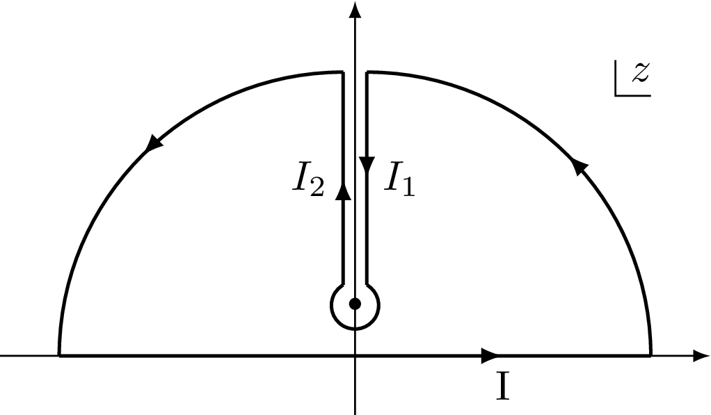
We choose the integration contour for the first term as depicted in the Fig 1. Applying the Cauchy integral formula

$$\int_{-\infty}^{\infty}\mathrm{d}y\,e^{-2\mathrm{i}\pi py}\frac{1}{\left(y+\mathrm{i}n\tau_{2}\right)^{s}}=I=-I_{1}-I_{2}\qquad(\text{for }p<0\text{ and }n<0)\text{ ,}$$

(25)

where

	$\displaystyle I_{1}$	$\displaystyle=\mathrm{i}\int_{\infty}^{-n\tau_{2}}\mathrm{d}x\,e^{2\pi px}\frac{e^{-\mathrm{i}\pi s/2}}{(x+n\tau_{2})^{s}}=-\mathrm{i}e^{-\mathrm{i}\pi s/2}e^{-2np\pi\tau_{2}}(-p)^{s-1}(2\pi)^{s-1}\Gamma(1-s)$
	$\displaystyle I_{2}$	$\displaystyle=\mathrm{i}\int_{-n\tau_{2}}^{\infty}\mathrm{d}x\,e^{2\pi px}\frac{e^{\mathrm{i}3\pi s/2}}{(x+n\tau_{2})^{s}}=\mathrm{i}e^{\mathrm{i}3\pi s/2}e^{-2np\pi\tau_{2}}(-p)^{s-1}(2\pi)^{s-1}\Gamma(1-s)\text{ .}$

So we get

$$I=-e^{\mathrm{i}\pi(1-s)/2}(e^{2\mathrm{i}\pi s}-1)e^{-2np\pi\tau_{2}}(-2p\pi)^{s-1}\Gamma(1-s)\text{ .}$$

Similarly for $n>0$ and $p>0$, we obtain

$$\int_{-\infty}^{\infty}\mathrm{d}y\,e^{-2\mathrm{i}\pi py}\frac{1}{\left(y+\mathrm{i}n\tau_{2}\right)^{s}}=-e^{-\mathrm{i}\pi(1-s)/2}(e^{-2\mathrm{i}\pi s}-1)e^{-2np\pi\tau_{2}}(2\pi p)^{s-1}\Gamma(1-s)\text{ .}$$

(26)

For the case $p=0$, the direct evaluation of the first line of eq.(24) yields,

	$\displaystyle\tilde{I}(\tau_{2},s)$	$\displaystyle\equiv\int_{0}^{1}\mathrm{d}y\,\sum_{m}\frac{1}{\left(m+y+\mathrm{i}n\tau_{2}\right)^{s}}$
		$\displaystyle=\frac{1}{1-s}\left(\sum_{m}\frac{1}{(m+1+\mathrm{i}n\tau_{2})^{s-1}}-\sum_{m}\frac{1}{(m+\mathrm{i}n\tau_{2})^{s-1}}\right)=0\text{ .}$

Thus, Eq. (24) yields

		$\displaystyle\sum_{n>0}\sum_{p>0}-e^{-\mathrm{i}\pi(1-s)/2}(e^{-2\mathrm{i}\pi s}-1)e^{-2np\pi\tau_{2}}(2\pi p)^{s-1}\Gamma(1-s)e^{2\mathrm{i}\pi pn\tau_{1}}$
		$\displaystyle\qquad\qquad+\sum_{n<0}\sum_{p<0}-e^{\mathrm{i}\pi(1-s)/2}(e^{2\mathrm{i}\pi s}-1)e^{-2np\pi\tau_{2}}(-2p\pi)^{s-1}\Gamma(1-s)e^{2\mathrm{i}\pi pn\tau_{1}}$
		$\displaystyle\qquad=\sum_{n>0}\sum_{p>0}\frac{2}{(2\pi)^{1-s}}\left(\cos(\frac{\pi(1-s)}{2})-\cos(\frac{\pi(1+3s)}{2})\right)e^{-2np\pi\tau_{2}}p^{s-1}\Gamma(1-s)e^{2\mathrm{i}\pi pn\tau_{1}}$
		$\displaystyle\qquad=2s\sum_{n>0}\sum_{p>0}(p)^{-1}e^{2\mathrm{i}\pi pn\tau}+O(s^{2})$
		$\displaystyle\qquad=-2s\ln\prod_{n>0}(1-q^{n})+O(s^{2})\text{ .}$

Putting them all together we can now write Eq.(23) as

$$G(s)=\left(\frac{\sqrt{\pi}}{\sqrt{2}\tau_{2}}\right)^{-s}\left[(1+(-1)^{-s})\zeta(s)-2s\ln\prod_{n>0}(1-q^{n})\right]+O(s^{2})\text{ .}$$

(27)

We thus obtain the partition function

	$\displaystyle Z(\tau)$	$\displaystyle=\sqrt{A}\exp G^{\prime}(0)=\sqrt{\tau_{2}}(-1)^{1/2}\frac{1}{\sqrt{8\pi}\tau_{2}}\prod_{n>0}(1-q^{n})^{-2}$
		$\displaystyle=\frac{\mathrm{i}}{\sqrt{8\pi\tau_{2}}}\prod_{n>0}(1-q^{n})^{-2}\text{ .}$		(28)

We now integrate out variable $\tau$ in the expression (28). To carry out this integration, we shall integrate first over $\tau_{1}$. Since only the infinite product has dependence on $\tau_{1}$, this integral simplifies to

	$\displaystyle Z(\tau_{2})$	$\displaystyle=\int_{-1/2}^{1/2}\mathrm{d}\tau_{1}\,Z(\tau)=\frac{\mathrm{i}}{\sqrt{8\pi\tau_{2}}}\int_{-1/2}^{1/2}\mathrm{d}\tau_{1}\,\prod_{n>0}(1-q^{n})^{-2}$
		$\displaystyle=\frac{\mathrm{i}}{\sqrt{8\pi\tau_{2}}}\int_{-1/2}^{1/2}\mathrm{d}\tau_{1}\,\left(\sum_{n=0}^{\infty}p(n)q^{n}\right)^{2}\text{ ,}$		(29)

where $p(n)$ is the partition number of $n$. Since for $|q|<1$, the power series on the r.h.s. of eq.(29) converges, we have, for any nonzero integer $m$,

$$\int_{-1/2}^{1/2}\mathrm{d}\tau_{1}\,q^{m}=\int_{-1/2}^{1/2}\mathrm{d}\tau_{1}\,e^{2m\pi i\tau_{1}}e^{-2m\pi\tau_{2}}=0\text{ .}$$

(30)

So we obtain the zero point one-loop amplitude for the null string

$$A_{\text{one-loop}}=\int_{0}^{\infty}(Z(\tau_{2}))^{d}\mathrm{d}\tau_{2}=\int_{0}^{\infty}\mathrm{d}\tau_{2}\,(\frac{\mathrm{i}}{\sqrt{8\pi\tau_{2}}})^{d}\text{ .}$$

(31)

For comparison, we also give the partition function for massless particles. As mentioned in the beginning of this section, the partition function for this case is just the one-loop vacuum bubble, given by

	$\displaystyle A(\text{vac bubble})$	$\displaystyle=\int\frac{\mathrm{d}^{d}k}{(2\pi)^{d}}\frac{1}{k^{2}}=\int\frac{\mathrm{d}^{d}k}{(2\pi)^{d}}\int_{0}^{\infty}\mathrm{d}l\exp(-k^{2}l)$
		$\displaystyle=\mathrm{i}\int_{0}^{\infty}\mathrm{d}l\,(2\pi l)^{-d/2}\text{ ,}$		(32)

where we have used the method of Schwinger proper time, and the factor $\mathrm{i}$ in front of the last line arises form the Wick rotation. This can be considered as the sum over all particle paths with the topology of a circle, $l$ being the length of the circle.

We find, apart from some adjustable constant factors, the zero point one-loop amplitude (31) for the null string is the same as that for the massless particles. This strongly supports that $\tau_{2}$ is identical to the Schwinger proper time in point particle field theory.

It was shown in [9] that for supergravity the factor $\mathcal{I}(\tau,\{z_{i}\})$ in eq.(11) is independent of $z_{i}$ and $\tau$ when $n=4$, as in conventional string theory. For simplicity, we choose $\mathcal{I}=1$ in this case.

In fact it is not easy to solve the scattering equations on the torus. In the previous section, we have shown that the partition function can be simplified by first integrating out the $\tau_{1}$ variable. We expect that the same kind of simplification will occur in the computation of amplitudes. Before proceeding, we specify the domain of $z$-integration to be $\left|\operatorname{Re}z\right|<1/2$ and $0<\operatorname{Im}z<\tau_{2}$, so that the integration over $\tau_{1}$ is straightforward. Using the infinite product form of $\theta_{1}$,

$$\theta_{1}(z|\tau)=2q^{1/8}\sin(\pi z)\prod_{m=1}^{\infty}(1-q^{m})(1-e^{2\pi iz}q^{m})(1-e^{-2\pi iz}q^{m})$$

we find that $G(z)$ can be written as

	$\displaystyle G(z)$	$\displaystyle=(\bar{\tau}-\tau)\partial_{\tau}\ln\theta_{1}(z|\tau)+(\bar{z}-z)\partial_{z}\ln\theta_{1}(z|\tau)+\frac{\pi\mathrm{i}}{\bar{\tau}-\tau}(\bar{z}-z)^{2}$
		$\displaystyle=\frac{\pi\tau_{2}}{2}+(\bar{z}-z)\pi\cot(\pi z)-\frac{\pi}{2\tau_{2}}(\bar{z}-z)^{2}+O(q)\text{.}$		(33)

Integrating out $\tau_{1}$ first, we get the expression for the partial amplitude

$$A(k_{1},\cdots,k_{n})=C\int_{0}^{\infty}\mathrm{d}\tau_{2}(\tau_{2})^{-d/2}\prod_{\mu=2}^{n}\int\mathrm{d}z_{\mu}\mathrm{d}\bar{z}_{\mu}\exp(-\sum_{i<j}^{n}k_{i}\cdot k_{j}\tilde{G}_{ij})$$

(34)

where

$$\tilde{G}_{ij}=\frac{\pi\tau_{2}}{2}+(\bar{z}_{ij}-z_{ij})\pi\cot(\pi z_{ij})-\frac{\pi}{2\tau_{2}}(\bar{z}_{ij}-z_{ij})^{2}\text{ ,}$$

(35)

$C$ is an overall constant, $z_{ij}\equiv z_{i}-z_{j}$ and $n=4$ for the present example. Note that the first term on the r.h.s. of the eq.(35) actually has no contribution to the amplitude since $\sum_{ij}k_{i}\cdot k_{j}=0$.

We can set $z_{1}=0$ by making use of the two conformal Killing vectors on the torus. Then there are three possible ways in dividing the integration region up to topological equivalence: (i) $0=\operatorname{Im}z_{1}<\operatorname{Im}z_{2}<\operatorname{Im}z_{3}<\operatorname{Im}z_{4}<\tau_{2}$, (ii) $0=\operatorname{Im}z_{1}<\operatorname{Im}z_{2}<\operatorname{Im}z_{4}<\operatorname{Im}z_{3}<\tau_{2}$, and (iii) $0=\operatorname{Im}z_{1}<\operatorname{Im}z_{4}<\operatorname{Im}z_{2}<\operatorname{Im}z_{3}<\tau_{2}$. (As a matter of fact, there are six ways to split the integration region, but the other three cases give the same contributions as those three mentioned above, as will become clear in what follows.) Since the difference among the cases (i), (ii) and (iii) is just the interchange of the momentum indices, it is sufficient to consider only the case (i). Note that, $\tilde{G}_{ij}$ is regular at $z_{i}=z_{j}$, since it is suppressed by $\operatorname{Im}z_{i}-\operatorname{Im}z_{j}$, so that the multi-integral in eq.(34) is well defined. We will show that Eq. (34) give the amplitude for the Feynman diagrams in Fig.2. More precisely, the case (i) corresponds to figure (a), the case (ii) to figure (b), and the case (iii) to figure (c). In what follows, we will focus on the case (i).

Before doing the integration in Eq. (34), let us review the Schwinger parametrization in field theory. In terms of Schwinger parameters $s_{i}$ ($i=1,2,3,4$) the amplitude for massless particles represented by figure (a) can be written as

		$\displaystyle\int\frac{\mathrm{d}^{d}p}{(2\pi)^{d}}\frac{1}{p^{2}(p+k_{1})^{2}(p+k_{1}+k_{2})^{2}(p-k_{4})^{2}}$
		$\displaystyle\qquad=\int\frac{\mathrm{d}^{d}p}{(2\pi)^{d}}\int_{0}^{\infty}\mathrm{d}s_{1}\cdots\int_{0}^{\infty}\mathrm{d}s_{4}$
		$\displaystyle\qquad\quad\exp\left[-s_{4}p^{2}-s_{1}(p+k_{1})^{2}-s_{2}(p+k_{1}+k_{2})^{2}-s_{3}(p-k_{4})^{2}\right]$
		$\displaystyle\qquad=C_{1}\prod_{i=1}^{4}\int_{0}^{1}\mathrm{d}\alpha_{i}\,\delta\left(\sum_{i=1}^{4}\alpha_{i}-1\right)\int_{0}^{\infty}\mathrm{d}\tau_{2}(\tau_{2})^{3-d/2}\exp\left[\tau_{2}(\ell^{2}-2\alpha_{2}k_{1}\cdot k_{2})\right]\text{ ,}$		(36)

with

	$\displaystyle\ell$	$\displaystyle=k_{1}(\alpha_{1}+\alpha_{2}+\alpha_{3})+k_{2}(\alpha_{2}+\alpha_{3})+k_{3}\alpha_{3}\text{ ,}$		(37)
	$\displaystyle\tau_{2}$	$\displaystyle=s_{1}+s_{2}+s_{3}+s_{4}\text{ ,}$		(38)
	$\displaystyle\alpha_{i}$	$\displaystyle=\frac{s_{i}}{\tau_{2}}\text{ ,}\qquad\quad i=1,2,3,4\text{ ,}$		(39)
	$\displaystyle k_{i}^{2}$	$\displaystyle=0\text{ ,}\qquad\quad i=1,2,3,4\text{ .}$

Here $C_{1}$ is the integration constant, and we have eliminated $k_{4}$ by the conservation of momentum. In this formalism, the geometric meaning of each parameter is clear. $\tau_{2}$ is the proper time of the whole loop, and $\alpha_{i}\tau_{2}$ is the proper time of the world line connecting the point $i$ and the point $i+1$. We use the same parameter $\tau_{2}$ as what is used in the string theory because they play the same role. In what follows we will show the connection between $\alpha_{i}$ and coordinates $z_{i}$ of the vertex operators, or more specifically, the connection between $\alpha_{i}$ and $\operatorname{Im}z_{i}$.

We now turn to the integration in Eq. (34). For our purpose, we should integrate over $\operatorname{Re}z_{i}$ first. It is convenient to define $\sigma_{i}=\exp(2\pi\mathrm{i}z_{i})$. We denote the phase argument of $\sigma_{i}$ as $\phi_{i}$, $\operatorname{Re}z_{i}$ as $x_{i}$, and $\operatorname{Im}z_{i}$ as $y_{i}$, respectively. In terms of $\sigma_{i}$, Eq. (34) reads

$$A(k_{1},\cdots,k_{n})=C\int_{0}^{\infty}\mathrm{d}\tau_{2}(\tau_{2})^{-d/2}\prod_{\mu=2}^{4}\int\frac{\mathrm{d}\phi_{i}\mathrm{d}\left|\sigma_{i}\right|}{4\pi^{2}\left|\sigma_{i}\right|}\exp\left(-\sum_{i<j}k_{i}\cdot k_{j}\tilde{G}_{ij}\right)\text{ ,}$$

(40)

where

$$\tilde{G}_{ij}=\frac{1}{2}\ln\left|\frac{\sigma_{i}}{\sigma_{j}}\right|^{2}\frac{\sigma_{i}+\sigma_{j}}{\sigma_{i}-\sigma_{j}}-\frac{\pi}{2\tau_{2}}\left(\frac{1}{2\pi\mathrm{i}}\ln\left|\frac{\sigma_{i}}{\sigma_{j}}\right|^{2}\right)^{2}\text{ .}$$

(41)

The integrations over $x_{i}$’s are equivalent to those over $\phi_{i}$, so we just need to consider the first term on the r.h.s. of Eq.(41). In the case (i), for any $i<j$, we have $y_{i}<y_{j}$ and hence $|\sigma_{i}|>|\sigma_{j}|$, thus we obtain the power series expression for the first term of $\tilde{G}_{ij}$:

$$\frac{\sigma_{i}+\sigma_{j}}{\sigma_{i}-\sigma_{j}}=1+2\sum_{n=1}^{\infty}\left|\frac{\sigma_{j}}{\sigma_{i}}\right|^{n}e^{\mathrm{i}n(\phi_{j}-\phi_{i})}\text{ .}$$

Integrating out $\phi_{i}$’s we derive the reduced effective Green functions

$$\tilde{G}_{ij}^{\text{eff}}=\frac{1}{2}\ln\left|\frac{\sigma_{i}}{\sigma_{j}}\right|^{2}-\frac{\pi}{2\tau_{2}}\left(\frac{1}{2\pi\mathrm{i}}\ln\left|\frac{\sigma_{i}}{\sigma_{j}}\right|^{2}\right)^{2}\text{ .}$$

Note that $\tilde{G}_{ij}^{\text{eff}}$ are not symmetric with respect to indices $i$ and $j$ any longer - the order of indices is now important.

Now after integrating out the coordinates $x_{i}$’s in Eq. (34), we get

	$\displaystyle A(k_{1},\cdots,k_{n})$	$\displaystyle=C\int_{0}^{\infty}\mathrm{d}\tau_{2}(\tau_{2})^{-d/2}$
		$\displaystyle\quad\times\prod_{\mu=2}^{4}\int_{0}^{\tau_{2}}\mathrm{d}y_{\mu}\exp\left(-\sum_{i<j}k_{i}\cdot k_{j}\left[y_{ij}+\frac{1}{\tau_{2}}(y_{ij})^{2}\right]2\pi\right)\prod_{i}\theta(y_{i+1,i})\text{ ,}$		(42)

where step function $\theta(s)$ has the value $+1$ for $s>0$ and $0$ for $s<0$ and $y_{ij}\equiv y_{i,j}\equiv y_{i}-y_{j}$. For comparison with the Schwinger form in field theory, it is convenient to make some variable substitutions. First, rescaling the $y_{i}$’s by a factor of $\tau_{2}$, we get

	$\displaystyle A(k_{1},\cdots,k_{n})=$	$\displaystyle C\int_{0}^{\infty}\mathrm{d}\tau_{2}(\tau_{2})^{-d/2+3}$
		$\displaystyle\times\prod_{\mu=2}^{4}\int_{0}^{1}\mathrm{d}y_{\mu}\exp\left(-\sum_{i<j}k_{i}\cdot k_{j}\left[y_{ij}+(y_{ij})^{2}\right]2\pi\tau_{2}\right)\prod_{i}\theta(y_{i+1,i})\text{ .}$		(43)

Next, rescaling $\tau_{2}$ by a factor of $1/2\pi$, this gives an extra factor $(2\pi)^{4-d/2}$ which can be absorbed into the overall constant $C$. Then we obtain the final result of the amplitude

	$\displaystyle A(k_{1},\cdots,k_{n})=$	$\displaystyle C\int_{0}^{\infty}\mathrm{d}\tau_{2}(\tau_{2})^{-d/2+n-1}$
		$\displaystyle\times\prod_{\mu=2}^{n}\int_{0}^{1}\mathrm{d}y_{\mu}\exp\left(-\sum_{i<j}k_{i}\cdot k_{j}\left[y_{ij}+(y_{ij})^{2}\right]\tau_{2}\right)\prod_{i}\theta(y_{i+1,i})\text{ ,}$		(44)

with $n=4$. Up to an overall constant, Eqs. (36) and (44) are equal after identifying the string variables $y_{ij}$ to the particle variables $\alpha_{i}$:

$$\alpha_{i}=y_{i+1}-y_{i},\quad i=1,\cdots,n,\quad\text{letting}\quad y_{n+1}=1\text{ ,}$$

(45)

here we specify ourselves to the case $n=4$. Using the identification (45) in Eq. (44), and eliminating $k_{4}$ by the conservation of momentum $\sum k_{i}=0$, $k_{2}\cdot k_{3}$ by the Mandelstam relation $k_{1}\cdot k_{2}+k_{1}\cdot k_{3}+k_{2}\cdot k_{3}=0$, we obtain the expression for the amplitude corresponding to figure (a) in Fig.2

	$\displaystyle A(k_{1},\cdots,k_{n})$	$\displaystyle=C\int_{0}^{\infty}\mathrm{d}\tau_{2}(\tau_{2})^{-d/2+3}\prod_{i=1}^{4}\int_{0}^{1}\mathrm{d}\alpha_{i}\,\delta\left(\sum_{i=1}^{4}\alpha_{i}-1\right)$
		$\displaystyle\quad\exp\left\{\left[\left((\alpha_{1}+\alpha_{2})(\alpha_{2}+\alpha_{3})-\alpha_{2}\right)2k_{1}\cdot k_{2}+2\alpha_{1}\alpha_{3}k_{1}\cdot k_{3}\right]\tau_{2}\right\}\text{ .}$		(46)

It is clear now that if we specify the order of $y_{i}$’s along the integration interval, we can obtain the amplitude for the associated Feynman diagram. There are six different orders for $z_{i}$ since the coordinate $z_{1}$ is fixed. These six different orders reduce to three Feynman diagrams up to the topological equivalence.

References

- (1) F. Cachazo, S. He and E. Y. Yuan, Scattering of massless particles in arbitrary dimensions, Phys.Rev.Lett. 113 (2014) 171601, [arXiv:1307.2199].
- (2) F. Cachazo, S. He and E. Y. Yuan, Scattering of massless particles: scalars, gluons and gravitons, JHEP 2014 (2014) 33, [arXiv:1309.0885].
- (3) F. Cachazo, S. He and E. Y. Yuan, Scattering equations and kawai-lewellen-tye orthogonality, Phys. Rev. D90 (2014) 065001, [arXiv:1306.6575].
- (4) L. Mason and D. Skinner, Ambitwistor strings and the scattering equations, JHEP 2014 (2014) 48, [arXiv:1311.2564].
- (5) E. Casali and P. Tourkine, On the null origin of the ambitwistor string, JHEP 2016 (2016) 36, [arXiv:1606.05636].
- (6) T. Adamo, E. Casali and D. Skinner, Ambitwistor strings and the scattering equations at one loop, JHEP 2014 (2014) 104, [arXiv:1312.3828].
- (7) Y. Geyer, L. Mason, R. Monteiro and P. Tourkine, One-loop amplitudes on the riemann sphere, JHEP 2016 (2016) 114, [arXiv:1511.06315].
- (8) Y. Geyer, L. Mason, R. Monteiro and P. Tourkine, Loop integrands for scattering amplitudes from the riemann sphere, Phys.Rev.Lett. 115 (2015) 121603, [arXiv:1507.00321].
- (9) E. Casali and P. Tourkine, Infrared behaviour of the one-loop scattering equations and supergravity integrands, JHEP 2015 (2015) 13, [arXiv:1412.3787].
- (10) S. He and E. Y. Yuan, One-loop scattering equations and amplitudes from forward limit, Phys. Rev. D92 (2015) 105004, [arXiv:1508.06027].
- (11) F. Cachazo, S. He and E. Y. Yuan, One-loop corrections from higher dimensional tree amplitudes, JHEP 2016 (2016) 8, [arXiv:1512.05001].
- (12) C. Baadsgaard, N. E. J. Bjerrum-Bohr, J. L. Bourjaily, P. H. Damgaard and B. Feng, Integration rules for loop scattering equations, JHEP 2015 (2015) 80, [arXiv:1508.03627].
- (13) C. Baadsgaard, N. E. J. Bjerrum-Bohr, J. L. Bourjaily, S. Caron-Huot, P. H. Damgaard and B. Feng, New representations of the perturbative matrix, Phys. Rev. Lett. 116 (2016) 061601, [arXiv:1509.02169].
- (14) K. Ohmori, Worldsheet geometries of ambitwistor string, arXiv:1504.02675v2.
- (15) Z. Bern and D. A. Kosower, The computation of loop amplitudes in gauge theories, Nucl. Phys. B379 (1992) 451–561.
- (16) A. Karlhede and U. Lindstrom, The Classical Bosonic String in the Zero Tension Limit, Class. Quant. Grav. 3 (1986) L73-L75.
- (17) U. Lindström, B. Sundborg and G. Theodoridis, The zero tension limit of the superstring, Phys. Lett. B253 (1991) 319–323.
- (18) W. Siegel, Amplitudes for left-handed strings, arXiv:1512.02569.
- (19) O. Hohm, W. Siegel and B. Zwiebach, Doubled -geometry, JHEP 2014 (2014) 65, [arXiv:1306.2970].
- (20) Y. Li and W. Siegel, Chiral superstring and chy amplitude, arXiv:1702.07332.
- (21) F. Lizzi, B. Rai, G. Sparano and A. Srivastava, Quantization of the null string and absence of critical dimensions, Phys. Lett. B182 (1986) 326–330.
- (22) J. Gamboa, C. Ramírez and M. Ruiz-Altaba, Null spinning strings, Nucl. Phys. B338 (1990) 143–187.
- (23) J. Isberg, U. Lindström, B. Sundborg and G. Theodoridis, Classical and quantized tensionless strings, Nucl. Phys. B411 (1994) 122-156. [arXiv:hep-th/9307108].
- (24) J. Gamboa, C. Ramírez and M. Ruiz-Altaba, Quantum null (super)strings, Phys. Lett. B225 (1989) 335-339.
- (25) Y.-t. Huang, W. Siegel and E. Y. Yuan, Factorization of chiral string amplitudes, JHEP 2016 (2016) 101, [arXiv:1603.02588].
- (26) P. Francesco, P. Mathieu and D. Sénéchal, Conformal field theory. Springer Science & Business Media, 2012.
- (27) M. Yu, C. Zhang and Y.-Z. Zhang, Operator formalism for null string at one loop, to appear .