Blind Signal Detection in Massive MIMO: Exploiting the Channel Sparsity

The remainder of this paper is organized as follows. In Section II, we introduce a sparse channel model for the massive MIMO system. In Section III, we present upper and lower bounds of the capacity of the massive MIMO system. In Section IV, we analyze the DoF of the proposed scheme. In Section V, we develop a message-passing based detection algorithm to jointly detect the data of users and the channel matrix. Numerical results are presented in Section VI to verify the effectiveness of our proposed scheme. Finally, we conclude the paper in Section VII.

Regular letters, lowercase bold letters, and capital bold letters represent scalars, vectors, and matrices, respectively. $\mathbb{C}$ denotes the complex field; the superscripts $(\cdot)^{\text{H}}$, $(\cdot)^{*}$, $(\cdot)^{\text{T}}$, and $(\cdot)^{-1}$ represent the conjugate transpose, conjugate, transpose, and the inverse of a matrix, respectively; $|\cdot|,\|\cdot\|_{1},\|\cdot\|_{2}$, and $\|\cdot\|_{F}$ represent the absolute value, the $\ell_{1}$-norm, the $\ell_{2}$-norm, and the Frobenius norm, respectively; $\mathsf{E}[\cdot]$, $\det(\cdot)$, and $\log(\cdot)$ represents the expectation, the determinant, and the logarithm function; $\text{diag}\{\mathbf{a}\}$ represents the diagonal matrix with the diagonal specified by $\mathbf{a}$; $\lceil a\rceil$ represents the minimum integer larger than $a$. For an integer $N$, $\mathcal{I}_{N}$ denotes the set of integers from $1$ to $N$. The notation $\propto$ denotes equality up to a constant scaling factor. The notation $a\lesssim b$ means $\limsup_{b\rightarrow\infty}\frac{a}{b}\leq c$, where $c>0$ is a constant. Similarly, $a\gtrsim b$ means $\limsup_{a\rightarrow\infty}\frac{b}{a}\leq c$.

We now present a sparse channel model for massive MIMO systems by following the approach in [21]. Consider a massive MIMO channel with $K$ single-antenna transmitters and a receiver deployed with uniform linear array (ULA) of $N$ antennas. By massive MIMO, we assume $N\gg K\gg 1$. This setting arises in practical scenarios, e.g., when a base station that deploys an array of a few hundred antennas communicates with tens of users. Let $L_{r}$ be the normalized length of the ULA.¹¹ 1 This means, the actual length of the ULA is $\lambda_{c}L_{r}$, where $\lambda_{c}$ is the wavelength. Then, the normalized interval between any two adjacent receive antennas is $\Delta_{r}=L_{r}/N$. Denote by $L_{k}$ the number of physical paths between transmitter $k$ and the receiver, by $\alpha_{l,k}$ the path gain of the $l$th path of transmit $k$, and by $\theta_{l,k}$ the AoA of the $l$th path of transmitter $k$. Then, the physical channel of a nonselective MIMO channel from transmitter $k$ to the receiver can be modeled by

where

represents the array steering vector for receiving a signal from transmitter $k$ in the direction given by $\theta_{k,l}$, and $\mathsf{j}=\sqrt{-1}$. By using the virtual representation method in [21], we can rewrite (1) as

where $\mathbf{A}_{r}=\left[\mathbf{a}_{r}\left(\arccos\frac{0}{L_{r}}\right),\ldots,\mathbf{a}_{r}\left(\arccos\frac{N-1}{L_{r}}\right)\right]\in\mathbb{C}^{N\times N}$ is a unitary matrix, and $\mathbf{h}_{k}$ is the $k$th column of $\mathbf{H}$ in (8). From (3), $\mathbf{h}_{k}=[h_{1,k},\cdots,h_{N,k}]^{\text{T}}$ can be treated as an equivalent channel of user $k$ in the angular domain, where $h_{n,k}$ is the aggregated gain of the physical paths of user $k$ within the resolution bin centered around $\arccos\frac{n}{L_{r}}$ in the angular domain. Denote by $\tilde{\mathbf{H}}=[\tilde{\mathbf{h}}_{1},\cdots,\tilde{\mathbf{h}}_{K}]$ the overall channel matrix. Then

where $\mathbf{H}=[\mathbf{h}_{1},\cdots,\mathbf{h}_{K}]$ is the projection of the channel in the angular domain.

We now describe the sparsity of $\mathbf{H}$ for massive MIMO systems. Recall that each $h_{n,k}$ is the aggregated channel gain of the physical paths of transmit terminal $k$ whose AoAs are within the $n$th resolution bin in the angular domain. It has been previously discussed in [15, 16, 18, 19] that a large portion of the elements of $\mathbf{H}$ are very close to zero, since the number of resolution bins of a massive antenna array usually far exceeds the number of physical paths of each user $k$, i.e., $N\gg L_{k}$. An example is illustrated in Fig. 1. These near-zero elements of $\mathbf{H}$ correspond to weak channel links, and can be essentially ignored in the transceiver design of a massive MIMO system.

Based on the above discussions, we henceforth assume that the massive MIMO channel is sparse, i.e., the sparsity level $\rho$ satisfies

where $\mathcal{S}$ is the support of the non-zero elements of $\mathbf{H}$, i.e.

and $|\mathcal{S}|$ represents the cardinality of the set $\mathcal{S}$.

The signal model of the massive MIMO system is presented as follows. The channel is assumed to be block-fading, i.e., the channel remains unchanged within the coherence time $T$. Then, for each transmission block of duration $T$, the received signal matrix is represented by

where $\tilde{\mathbf{Y}}\in\mathbb{C}^{N\times T}$ is the received signal over $T$ time slots, $\mathbf{X}\in\mathbb{C}^{K\times T}$ is the transmitted signal from all the $K$ transmit terminals, and $\tilde{\mathbf{W}}\in\mathbb{C}^{N\times T}$ is the additive white Gaussian noise with each element independently drawn from $\mathcal{CN}(0,\sigma^{2})$.

By left-multiplying $\tilde{\mathbf{Y}}$ with $\mathbf{A}_{r}^{\text{H}}$, we obtain the projection of the received signal in the angular domain as

where $\mathbf{Y}=\tilde{\mathbf{Y}}\mathbf{A}_{r}^{\text{H}}\in\mathbb{C}^{N\times T}$, and $\mathbf{W}=\tilde{\mathbf{W}}\mathbf{A}_{r}^{\text{H}}\in\mathbb{C}^{N\times T}$. Note that the elements of $\mathbf{W}$ are still independent and identically distributed Gaussian random variables with zero mean and variance $\sigma^{2}$. Let $\mathbf{x}_{k}\in\mathbb{C}^{T\times 1}$ be the transpose of the $k$th row of $\mathbf{X}$. We assume that the average transmission power of each transmit terminal is given by $\alpha_{k}P$, i.e.

where $\alpha_{k}\geq 0$ for $k\in\mathcal{I}_{K}$ satisfy $\sum_{k=1}^{K}\alpha_{k}=1$, and $P$ is the total power budget.

The system capacity of a massive MIMO system is given by

where the signal-to-noise ratio (SNR) is defined by $\mathsf{SNR}=\frac{P}{\sigma^{2}}$ and the maximization is taken over the distribution of $\mathbf{X}$, denoted by $p_{\mathbf{X}}(\mathbf{X})$, subject to the power constraint in (9).

We start with a capacity upper bound. Ideally, when the CSI is perfectly known at the receiver, the capacity of the channel (8) is given by the following theorem [32].

Lemma 1 gives a performance upper bound for the considered massive MIMO system. We will show that, with channel sparsity, the ideal capacity can be closely approached, especially in the high SNR regime.

We now introduce lower bounds to the system capacity in (10). In general, every realizable detection scheme for the system in (8) provides a lower bound to the system capacity in (10). As aforementioned, all the existing schemes for massive MIMO perform very far away from the ideal capacity given in Lemma 1, or in other words, the lower bounds provided by these schemes are very loose.

In this paper, we propose a blind detection scheme to directly estimate $\mathbf{H}$ and $\mathbf{X}$ from the observed signal matrix $\mathbf{Y}$ following the maximum a posteriori probability (MAP) principle. From the probability theory, the joint posterior probability density of $\mathbf{H}$ and $\mathbf{X}$ given $\mathbf{Y}$ is given by

where step $(a)$ follows from the Bayes’ rule and the fact that $\mathbf{H}$ and $\mathbf{X}$ are independent; the notation $\propto$ in step $(b)$ denotes equality up to a constant scaling factor; $p_{\mathbf{W}}(\cdot)$ in step $(c)$ denotes the probability density function (PDF) of noise $\mathbf{W}$; step $(d)$ follows from the fact that the elements of $\mathbf{W}$ are independently drawn from $\mathcal{CN}(0,\sigma^{2})$. Then, the MAP estimates of $\mathbf{H}$ and $\mathbf{X}$, denoted respectively by $\hat{\mathbf{H}}$ and $\hat{\mathbf{X}}$, are given by

The mutual information between $\hat{\mathbf{X}}$ and $\mathbf{X}$, denoted by $I(\hat{\mathbf{X}};\mathbf{X})$, provides a lower bound to the capacity in (10). The corresponding DoF lower bound is given by

The problem in (14) is in general difficult to solve, since the observed signal $\mathbf{Y}$ is a bilinear function of $\mathbf{H}$ and $\mathbf{X}$. Later, we will present a message-passing based algorithm to approximately solve (14), and will show that the lower bound provided by (14) is much tighter than the existing bounds.

To reveal the fundamental impact of channel sparsity on the DoF of a massive MIMO channel, we simplify (14) by ignoring $p_{\mathbf{X}}(\mathbf{X})$ (which is irrelevant to the channel sparsity) and replacing $p_{\mathbf{H}}(\mathbf{H})$ with a Laplace distribution $\exp\Big(-\frac{\lambda}{\sigma^{2}}\|\mathbf{H}\|_{1}\Big)$ (by following [33, 26, 35]), yielding²² 2 In (16), the $\ell_{1}$-norm of $\mathbf{H}$ is used as the penalty term in the optimization problem. This is widely used in the area of machine learning to find a sparse solution [35]. Note that $\lambda\|\mathbf{H}\|_{1}$ in (16b) implies a Laplace prior of $\mathbf{H}$. This explains why we choose a Laplace distribution for $p_{\mathbf{H}}(\mathbf{H})$ in (16a).

where $\lambda$ is a regularization parameter that controls the tradeoff between the channel sparsity and the signal detection quality. Note that $l_{1}$-norm minimization is a common practice to deal with signal sparsity in the area of sparse signal recovery [26, 30, 34, 33].

Similarly to (14), $I(\hat{\mathbf{X}};\mathbf{X})$ with $\hat{\mathbf{X}}$ given by (16) gives a lower bound to the capacity in (10) with corresponding achievable DoF given by (15). In the next section, we will analyze the DoF of the massive MIMO system based on the simplified problem in (16).

Note that whether a detection method is blind solely depends on the choice of the prior distribution $p_{\mathbf{X}}(\mathbf{X})$. For example, if a portion of the entries of $\mathbf{X}$ are perfectly known to the receiver, these entries are called pilot symbols and the corresponding scheme is training-based. Otherwise, $\mathbf{X}$ is said to be partially known to the receiver if $\mathbf{X}$ follows a certain distribution with a non-zero mean. In this paper, we focus on blind detection, in which $\mathbf{X}$ is unknown to the receiver. In other words, $\mathbf{X}$ is a random matrix following a zero-mean distribution.

The blind detection problem formulated in (16) suffers from ambiguities in signal estimation. Specifically, the objective function in (16) is invariant to phase shifts and permutations of the rows of $\mathbf{X}$. Denote by $\mathbf{\Sigma}$ a diagonal matrix with phase shifts in the diagonal and by $\mathbf{\Pi}$ a permutation matrix. Then, the ambiguities are caused by the fact that if $(\hat{\mathbf{H}},\hat{\mathbf{X}})$ is a solution to (16), then $(\hat{\mathbf{H}}^{\prime}=\hat{\mathbf{H}}\mathbf{\Pi}^{-1}\mathbf{\Sigma}^{-1},\hat{\mathbf{X}}^{\prime}=\mathbf{\Sigma}\mathbf{\Pi}\hat{\mathbf{X}})$ is also a valid solution to (16). These ambiguities need to be appropriately handled in the transceiver design, as detailed in the subsequent sections.

Besides the above ambiguities, there is another ambiguity inherent to blind detection. Denote by $\mathcal{S}_{k}$ and $\mathcal{S}_{k^{\prime}}$ the supports of the non-zero elements of $\mathbf{h}_{k}$ and $\mathbf{h}_{k^{\prime}}$, respectively. We refer to $\mathcal{S}_{k}$ as the sparsity pattern of transmitter $k$. We now describe the sparsity-pattern collision problem by assuming $\mathcal{S}_{k}=\mathcal{S}_{k^{\prime}}$. Denote by $\mathbf{H}_{\{k,k^{\prime}\}}=[\mathbf{h}_{k},\mathbf{h}_{k^{\prime}}]$ and by $\mathbf{X}_{\{k,k^{\prime}\}}=[\mathbf{x}_{k},\mathbf{x}_{k^{\prime}}]^{\text{T}}$ the channel matrix and the signal matrix of transmitters $k$ and $k^{\prime}$, respectively. Then, the noise-free received signal, denoted by $\mathbf{Y}_{\{k,k^{\prime}\}}$, is given by

We construct an alternative factorization of $\mathbf{Y}_{\{k,k^{\prime}\}}$ as

where

and $a$ and $b$ are numbers with $a+b\neq 1$. Since the two users have a common support, i.e., $\mathcal{S}_{k}=\mathcal{S}_{k^{\prime}}$, we have $\|\tilde{\mathbf{H}}_{\{k,k^{\prime}\}}\|_{1}=\|\mathbf{H}_{\{k,k^{\prime}\}}\|_{1}$ in general. Together with (18), we conclude that the solution of (16) is not unique in the sense that if $\mathbf{H}_{\{k,k^{\prime}\}}$ and $\mathbf{X}_{\{k,k^{\prime}\}}$ is a solution to (16), then $\tilde{\mathbf{H}}_{\{k,k^{\prime}\}}$ and $\tilde{\mathbf{X}}_{\{k,k^{\prime}\}}$ is also a solution to (16). This problem is referred to as sparsity-pattern collision. In practice, sparsity-pattern collision arises when the sparsity patterns of two or more users are close to each other, resulting in a non-zero probability of detection failure. We will see in the next section that, the failure probability can be made arbitrarily small in the high SNR regime if $N$ is sufficiently large and the channel is sufficiently sparse.

In this section, we analyze the achievable DoF of the proposed blind detection scheme for the massive MIMO system. As aforementioned, the DoF of the massive MIMO system without exploiting the channel sparsity is given by $K(1-\frac{K}{T})$ [11, 14]. Intuitively, each receive antenna receives a signal mixture from $K$ transmit terminals, and therefore needs to use $K$ time slots to identify $K$ channel coefficients, which contributes to the fractional DoF gap of $\frac{K}{T}$ from the ideal DoF. The compressed-sensing based training schemes [21] can reduce the fractional DoF gap to $c\frac{K}{T}$, where $c$ is a constant coefficient between zero and one determined by the channel sparsity level $\rho$. In the following, we will show that the proposed blind detection scheme can further reduce the fractional DoF gap to $\frac{1}{T}$, which brings forward a significant step towards the understanding of the fundamental capacity of the massive MIMO system with channel sparsity.

Our analysis is based on the problem formulation in (16). The DoF characterizes the behaviour of the minimizer $(\hat{\mathbf{H}},\hat{\mathbf{X}})$ when the SNR goes to infinity, or equivalently, when the noise level $\sigma^{2}$ goes to zero. This means that we need to understand how a small perturbation of the additive noise $\mathbf{W}$ affects the minimizer $\hat{\mathbf{H}}$ and $\hat{\mathbf{X}}$, and how the system parameters, such as $N$, $K$, $T$, and $\rho$, interact with each other to guarantee the existence of the minimizer $(\hat{\mathbf{H}},\hat{\mathbf{X}})$ around the ground truth of $(\mathbf{H},\mathbf{X})$. Moreover, in the analysis, we need to appropriately handle the phase and permutation ambiguities as well as the sparsity pattern collision problem described in Section III-C.

We start with some regularity conditions.

Assumption 1 (Coefficient independence):

Assumption 2 (Coefficient boundedness):

where $\mathsf{P}(\cdot)$ represents the probability function.

The assumption in (21a) is reasonable since in practical systems the channel coefficients with $|h_{n,k}|<\epsilon$ can be ignored without compromising the system performance, provided that $\epsilon$ is sufficiently small. As for the assumption in (21b), the length of the channel vector $\mathbf{h}_{k}$ for each transmitter $k$ is uniformly bounded since the received signal power from each transmitter is always bounded due to channel attenuation.

Assumption 3 (Noise boundedness):

where $\mathbf{w}_{n}$ denotes the transpose of the $n$th row of $\mathbf{W}$.

This assumption can be approximately satisfied by the Gaussian noise drawn from $\mathcal{CN}(0,\sigma^{2})$. For example, for $M_{w}=\sqrt{3T\sigma^{2}}$, $\mathsf{P}\left(\|\mathbf{w}_{n}\|_{2}>M_{w}\right)$ is only $0.00135$. In fact, with an appropriately chosen $M_{w}$, $\mathsf{P}\left(\|\mathbf{w}_{n}\|_{2}>M_{w}\right)$ can be made arbitrarily small and thus can be ignored from a practical point of view.

The main results of the paper are presented here and their proofs are given in the next subsection.

Remark 1: In (23), $e^{-\eta}$ can be understood as the detection failure probability. The sparsity-pattern collision discussed in Section III-C is one factor to cause detection failure. Intuitively, in practical massive MIMO systems, the sparsity-pattern collision arises when users are geographically close to each other. Signals from co-located users undergo similar scattering, leading to similar AoAs at the receive antenna array and hence similar sparsity patterns in the angular domain. Increasing the number of antennas improves the AoA resolution of an antenna array, and therefore reduces the probability of sparsity-pattern collision as well as the detection failure probability $e^{-\eta}$. This explains why in Theorem 1 a larger $N$ allows a larger $\eta$ (and hence a smaller detection failure probability $e^{-\eta}$). The DoF lower bound in (23) can approach $K\left(1-\frac{1}{T}\right)$ arbitrarily closely provided that $N$ is sufficiently large.

Remark 2: From Theorem 1, our scheme achieves a DoF arbitrarily close to $K(1-1/T)$, provided that $N$ is sufficiently large and the channel is sufficiently sparse. Compared with the ideal case in (12), our scheme has a fractional DoF loss of $1/T$. This loss is caused by the phase ambiguity of $\mathbf{H}$ and $\mathbf{X}$ discussed in Section III-C. In other words, a fraction $1/T$ of DoF is required to eliminate the ambiguity. We emphasize that the fractional DoF loss $1/T$ is independent of $K$, which is the key advantage of the proposed blind detection scheme compared with other existing counterparts.

For simplicity, we assume that $\alpha_{1}=\alpha_{2}=\cdots=\alpha_{K}=1/K$, and that the elements of $\mathbf{X}$ are independently drawn from $\mathcal{CN}(0,P/K)$. The optimization of the power coefficients $\{\alpha_{k}\}$ and the distribution of $\mathbf{X}$ may lead to a better performance, but is out of the scope of this paper.

We focus on the lower bound in (16). From (16), we see that, if $(\hat{\mathbf{H}},\hat{\mathbf{X}})$ is a solution to (16), then any $(\hat{\mathbf{H}}\mathbf{\Pi}^{-1}\mathbf{\Sigma}^{-1},\mathbf{\Sigma}\mathbf{\Pi}\hat{\mathbf{X}})$ is also a valid solution to (16) with $\mathbf{\Sigma}$ being a diagonal matrix for phase ambiguity and $\mathbf{\Pi}$ being a permutation matrix for permutation ambiguity. By considering these inherent ambiguities, an estimate $\hat{\mathbf{X}}$ for (16) can be modeled by

where the estimation error $\mathbf{\Delta}$ is zero-mean and uncorrelated with $\mathbf{X}$. Note that $\mathbf{\Sigma}$ and $\mathbf{\Pi}$ are regarded as deterministic parameters unknown to the receiver. We have the following result.

From Lemma 2, we have $N\gtrsim(TK^{3}+\eta K^{2})\left(\frac{1}{\delta}\cdot\frac{M_{w}}{M_{h}}\right)^{2}$ and $\|\mathbf{\Delta}\|_{F}^{2}<\delta^{2}$, yielding

We now describe how to determine the diagonal matrix $\mathbf{\Sigma}$ in (24). We use one symbol in each $\mathbf{x}_{k}$ to estimate $\mathbf{\Sigma}$.³³ 3 For ease of analysis, we assume coherent detection for each $\mathbf{x}_{k}$ in the proof. That is, one symbol in each $\mathbf{x}_{k}$ is used to estimate $\Sigma_{k}$, and the estimated $\Sigma_{k}$ is then used to detect the rest of $\mathbf{x}_{k}$. We emphasize that non-coherent detection can also be used here. For example, differential coding can be used to remove the phase uncertainty caused by $\Sigma_{k}$. We conjecture that coherent and non-coherent detections achieve the same DoF, as motivated by the result in [14]. Without loss of generality, we assume that $x_{k,1}=\sqrt{\frac{P}{K}},k\in\mathcal{I}_{K}$ is known to the receiver, where $x_{k,1}$ is the first entry of $\mathbf{x}_{k}$. Denote by $\boldsymbol{\delta}_{k}$ the transpose of the $k$th row of $\mathbf{\Delta}$. Then, from (24), we obtain

where $\hat{x}_{k,1}$ denotes the $(k,1)$th element of $\hat{\mathbf{X}}$, $\Sigma_{k}$ represents the $k$th diagonal element of $\mathbf{\Sigma}$, $\pi(\cdot)$ is the permutation function corresponding to $\mathbf{\Pi}$, and $\delta_{\pi(k),1}$ is the first entry of $\boldsymbol{\delta}_{\pi(k)}$. Then, an estimate of $\Sigma_{k}$, denoted by $\hat{\Sigma}_{k}$, is given by

The corresponding estimation error is given by

Denote by $\tilde{\mathbf{x}}_{k}\triangleq[x_{k,2},\cdots,x_{k,T}]^{\text{T}}\in\mathbb{C}^{(T-1)\times 1}$, $\hat{\tilde{\mathbf{x}}}_{k}\triangleq[\hat{x}_{k,2},\cdots,\hat{x}_{k,T}]^{\text{T}}\in\mathbb{C}^{(T-1)\times 1}$, and $\tilde{\boldsymbol{\delta}}_{k}=[\delta_{k,2},\cdots,\delta_{k,T}]^{\text{T}}\in\mathbb{C}^{(T-1)\times 1}$. From (24), we have

where $\mathbf{v}_{k}\triangleq(\Sigma_{k}-\hat{\Sigma}_{k})\tilde{\mathbf{x}}_{\pi(k)}+\Sigma_{k}\tilde{\boldsymbol{\delta}}_{\pi(k)}$. The average variance of the entries of $\mathbf{v}_{k}$ is given by

where $\sigma_{\delta_{k}}^{2}$ is the average variance of the entries of $\boldsymbol{\delta}_{k}$, defined by

In (30), step $(a)$ follows from the fact that $\mathbf{X}$ and $\mathbf{\Delta}$ are zero-mean and uncorrelated; step $(b)$ follows from (31); step $(c)$ follows from (28). In general, $\mathbf{v}_{k}$ is correlated with the signal $\hat{\Sigma}_{k}\tilde{\mathbf{x}}_{\pi(k)}$, and is not necessarily Gaussian. From [37], the mutual information between $\hat{\tilde{\mathbf{x}}}_{k}$ and $\tilde{\mathbf{x}}_{k}$ is lower bounded by the case when $\mathbf{v}_{k}$ is independent and Gaussian. Then

where step $(a)$ follows from (27) and (29); step $(b)$ follows from (30); and step $(c)$ follows from the high SNR approximation. Then, we have

where step (a) follows from $\prod_{k=1}^{K}\sigma_{\delta_{\pi(k)}}^{2}\leq\left(\frac{\mathsf{E}[\|\mathbf{\Delta}\|_{F}^{2}]}{KT}\right)^{K}$ for $\sum_{k=1}^{K}\sigma_{\delta_{\pi(k)}}^{2}=\frac{\mathsf{E}[\|\mathbf{\Delta}\|_{F}^{2}]}{T}$, with the equality holds for $\sigma_{\delta_{1}}^{2}=\cdots=\sigma_{\delta_{K}}^{2}=\frac{\mathsf{E}[\|\mathbf{\Delta}\|_{F}^{2}]}{KT}$.

We now consider the impact of permutation $\mathbf{\Pi}$ in (24). From (29), we see that the receiver decodes each $\tilde{\mathbf{x}}_{\pi(k)}$ from $\hat{\tilde{\mathbf{x}}}_{\pi(k)}$. Since $\mathbf{\Pi}$ is unknown, the receiver needs to associate each decoded codeword to the corresponding transmitter. This can be done by inserting a transmitter label into each codeword. To identify $K$ transmitters, each label costs $\lceil\log K\rceil$ bits. Thus, an achievable rate of the system in (8) is given by

From (25), with a probability of at least $1-e^{-\eta}$, we obtain

Thus, we have

where

Since $M_{h}^{2}$ is a constant and $M_{w}^{2}$ is proportional to $\sigma^{2}$ (from Assumption 3 and the discussions therein), the DoF of the proposed scheme is bounded by

which completes the proof of Theorem 1.

In this section, we present a blind detection algorithm to realize the DoF advantage promised by our analysis in practical system settings. We focus on the problem in (14), which is in general difficult to solve optimally. As aforementioned, the blind detection problem under concern is very similar to the matrix factorization problem in sparse dictionary learning [26]. In the context of dictionary learning, the blind detection problem can be rephrased as to learn the dictionary $\mathbf{X}$ and the corresponding sparse representation $\mathbf{H}$. Dictionary learning algorithms, such as the K-SVD algorithm [28], the SPAMS algorithm [29], and the BiG-AMP algorithm [31], can be potentially applied to approximately solve (14). However, there is a notable difference in the system configuration between the massive MIMO system and a typical dictionary learning problem. In dictionary learning, the dictionary $\mathbf{X}$ is usually overcomplete, i.e., $T\leq K$, so as to allow more flexible dictionaries and richer data representation. However, in massive MIMO, the setting of $T>K$ is of more relevance since the coherence time $T$ is usually in hundreds and the number of users is usually in tens.

It is known that BiG-AMP is a state-of-the-art dictionary learning algorithm. However, when applied to solve (14), BiG-AMP does not perform well in practical systems where $T>K$. To address this issue, we propose to preprocess the observed signal matrix $\mathbf{Y}$ by projecting it onto the signal space $\mathbf{X}$ and then apply BiG-AMP to the image of the projection. In addition, we describe how to eliminate the phase and permutation ambiguities. The resulting algorithm, referred to as P-BiG-AMP, is presented in the following subsections. Note that we always assume $T>K$ in the subsequent discussions. For the case of $T\leq K$, we simply skip the signal projection operation and directly apply BiG-AMP to solve (14).

From (8), the noise-free received signal $\mathbf{HX}$ has the same row space as $\mathbf{X}$ does. Thus, the row space of $\mathbf{X}$ can be estimated based on $\mathbf{Y}$ as follows.

Let the singular value decomposition (SVD) of $\mathbf{Y}$ be

where $\mathbf{U}\in\mathbb{C}^{N\times N}$ and $\mathbf{V}\in\mathbb{C}^{T\times T}$ are unitary matrices, and $\mathbf{D}\in\mathbb{R}^{N\times T}$ is a diagonal matrix with diagonal elements arranged in a descend order. Then, we partition $\mathbf{V}$ as

where $\mathbf{V}_{1}\in\mathbb{C}^{T\times K}$ corresponds to the largest $K$ singular values, and $\mathbf{V}_{2}\in\mathbb{C}^{T\times(T-K)}$ corresponds to the other singular values. Note that the column space of $\mathbf{V}_{1}$ gives an estimate of the row space of $\mathbf{X}$.

We then project the observed signal $\mathbf{Y}$ onto the column space of $\mathbf{V}_{1}$, yielding

where $\mathbf{X}^{\prime}\triangleq\mathbf{X}\mathbf{V}_{1}\in\mathbb{C}^{K\times K}$ and $\mathbf{W}^{\prime}\triangleq\mathbf{W}\mathbf{V}_{1}\in\mathbb{C}^{N\times K}$. After projection, the average transmission power constraint for $\mathbf{X}^{\prime}$ is given by

where $\mathbf{x}_{k}^{\prime}\in\mathbb{C}^{K\times 1}$ is the transpose of the $k$th row of $\mathbf{X}^{\prime}$.

The next step is to factorize $\mathbf{Y}^{\prime}$ to obtain $\mathbf{H}$ and $\mathbf{X}^{\prime}$. Denote by $p_{\mathbf{X}^{\prime}}(\mathbf{X}^{\prime})$ the prior distribution of $\mathbf{X}^{\prime}$. Then, similar to (14), the blind detection problem can be written as

The BiG-AMP algorithm can then be directly used to solve the problem in (43).

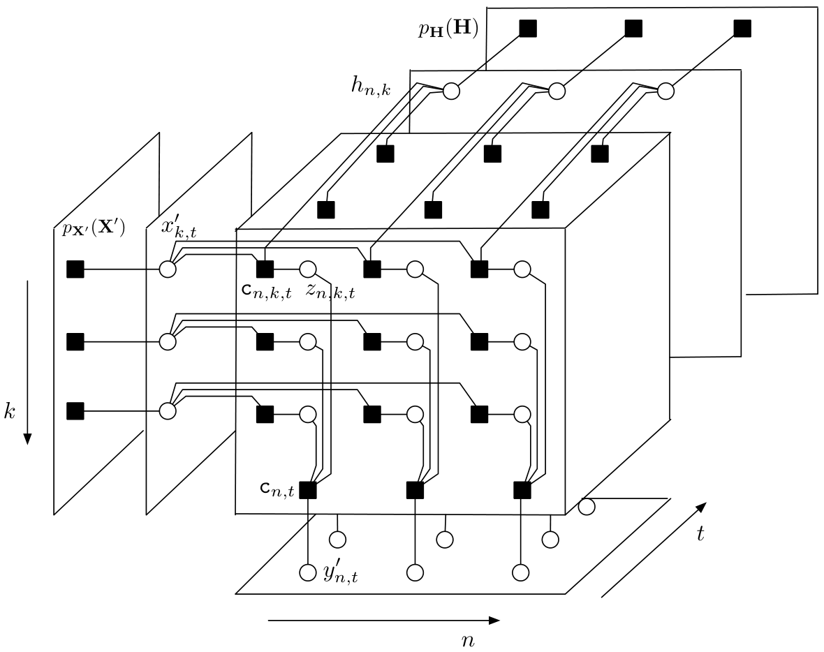
For completeness, we describe the BiG-AMP algorithm as follows. We start with the factor graph representation associated with the problem in (43). Denote by $y_{n,t}^{\prime}$ the $(n,t)$th element of $\mathbf{Y}^{\prime}$. Then, the system model (41) can be equivalently written as

where

with $x_{k,t}^{\prime}$ and $w_{n,t}^{\prime}$ are the $(k,t)$th and $(n,t)$th element of $\mathbf{X}^{\prime}$ and $\mathbf{W}^{\prime}$, respectively. With (44) and (45), we construct a factor graph illustrated in Fig. 2. The factor graph consists of two types of nodes: variable nodes and check nodes. Variable nodes include $\{h_{n,k}\}$, $\{x_{k,t}^{\prime}\}$, $\{z_{n,k,t}\}$, and $\{y_{n,t}^{\prime}\}$; check nodes include the $(n,t)$th equation in (44) (denoted by $\mathtt{c}_{n,t}$) for all $n\in\mathcal{I}_{N}$ and $t\in\mathcal{I}_{K}$, the $(n,k,t)$th equation in (45) (denoted by $\mathtt{c}_{n,k,t}$) for all $n\in\mathcal{I}_{N}$, $k\in\mathcal{I}_{K}$, and $t\in\mathcal{I}_{K}$, and also the prior distributions $p_{\mathbf{H}}(\mathbf{H})$ and $p_{\mathbf{X}^{\prime}}(\mathbf{X}^{\prime})$. In Fig. 2, all variable nodes appear as white circles and all check nodes appear as black boxes. There is an edge connection between a variable node and a check node when the variable node appears in the equation corresponding to the check node.

References

- [1] E. G. Larsson, O. Edfors, F. Tufvesson, and T. L. Marzetta, “Massive MIMO for next generation wireless systems,” IEEE Commun. Mag., vol. 52, no. 2, pp. 186-195, Feb. 2014.
- [2] T. L. Marzetta, “Noncooperative cellular wireless with unlimited numbers of base station antennas,” IEEE Trans. Wireless Commun., vol. 9, no. 11, pp. 3590-3600, Nov. 2010.
- [3] H. Q. Ngo, E. G. Larsson, and T. L. Marzetta, “Energy and spectral efficiency of very large multiuser MIMO systems,” IEEE Trans. Commun., vol. 61, no. 4, pp. 1436-1449, Apr. 2013.
- [4] J. Hoydis, S. T. Brink, and M. Debbah, “Massive MIMO in the UL/DL of cellular networks: How many antennas do we need?” IEEE J. Sel. Areas Commun., vol. 31, no. 2, pp. 160-171, Feb. 2013.
- [5] G. Geraci, R. Couillet, J. Yuan, M. Debbah, and I. B. Collings, “Large system analysis of linear precoding in MISO broadcast channels with confidential messages,” IEEE J. Sel. Areas Commun., vol. 31, no. 9, pp. 1660-1671, Sept. 2013.
- [6] Z. Fang, X. Yuan, X. Wang, and C. Li, “Nonregenerative cellular two-way relaying with large-scale antenna arrays,” IEEE Trans. on Veh. Technology, vol. 65, no. 7, pp. 4959-4972, Jul. 2016.
- [7] M.2083 : IMT Vision, “Framework and overall objectives of the future development of IMT for 2020 and beyond,” Sep. 2015.
- [8] C. Wang, F. Haider, X. Gao, X. You, Y. Yang, D. Yuan, H. Aggoune, H. Haas, S. Fletcher, and E. Hepsaydir, “Cellular architecture and key technologies for 5G wireless communication networks,” IEEE Communications Magazine, vol. 52, no. 2, pp. 122-130, Feb. 2014.
- [9] M. Coldrey (Tapio) and P. Bohlin, “Training-based MIMO systems-part I: performance comparison,” IEEE Trans. Signal Process., vol. 55, no. 11, pp. 5464-5476, Nov. 2007.
- [10] X. Yuan, C. Fan, and Y. Zhang, “Fundamental limits of training-based multiuser MIMO systems,” available at: http://arxiv.org/abs/1511.08977.
- [11] B. Hassibi and B. Hochwald, “How much training is needed in multiple antenna wireless links?” IEEE Trans. Inf. Theory, vol. 49, no. 4, pp. 951-963, Apr. 2003.
- [12] B. Muquet, M. De Courville, and P. Duhamel, “Subspace-based blind and semi-blind channel estimation for OFDM systems,” IEEE Trans. Signal Process., vol. 50, no. 7, pp. 1699-1712, Jul. 2002.
- [13] H. Q. Ngo and E. G. Larsson, “EVD-based channel estimation in multicell multiuser MIMO systems with very large antenna arrays,” in Proc. IEEE Int. Conf. Acoust. Speech Signal Process. (ICASSP), 2012, pp. 3249-3252.
- [14] L. Zheng, and D. N. C. Tse, “Communication on the Grassmann manifold: A geometric approach to the noncoherent multiple-antenna channel,” IEEE Trans. Inf. Theory, vol. 48, no. 2, pp. 359-383, Feb. 2002.
- [15] Z. Yan, M. Herdin, A. M. Sayeed, and E. Bonek, “Experimental study of MIMO channel statistics and capacity via the virtual channel representation,” Univ. Wisconsin-Madison, Madison, Tech. Rep., Feb. 2007.
- [16] A. M. Sayeed, “Deconstructing multiantenna fading channels,” IEEE Trans. Signal Process., vol. 50, no. 10, pp. 2563-2579. Oct. 2002.
- [17] M. K. Samimi and T. S. Rappaport, “3-d millimeter-wave statistical channel model for 5G wireless system design,” IEEE Trans. Microwave Theory and Techniques, vol. 64, no. 7, pp. 2007-2225, Jul. 2016.
- [18] L. Vuokko, V.-M. Kolmonen, J. Salo, and P. Vainikainen, “Measurement of large-scale cluster power characteristics for geometric channel models,” IEEE Trans. Antennas and Propagation, vol. 55, no. 11, pp. 3361-3365, Nov. 2007.
- [19] N. Czink, X. Yin, H. Ozcelik, M. Herdin, E. Bonek, and B. H. Fleury, “Cluster characteristics in a MIMO indoor propagation environment,” IEEE Trans. Wireless Commun., vol. 6, no. 4, pp. 1465-1475, Apr. 2007.
- [20] H. Yin, D. Gesbert, M. Filippou, and Y. Liu, “A coordinated approach to channel estimation in large-scale multiple antenna systems,” IEEE J. Sel. Areas Commun., vol. 31, no. 2, pp. 264-273, Feb. 2013.
- [21] W. U. Bajwa, J. Haupt, A. M. Sayeed, and R. Nowak, “Compressed channel sensing: A new approach to estimating sparse multipath channels,” IEEE Proceedings, vol. 98, no. 6, pp. 1058-1076, Jun. 2010.
- [22] X. Rao, and V. K. N. Lau, “Distributed compressive CSIT estimation and feedback for FDD multi-user massive MIMO systems,” IEEE Trans. Signal Process., vol. 62, no. 12, pp. 3261-3271, Jun. 2014.
- [23] M. Masood, L. H. Afify, and T. Y. Al-Naffouri, “Efficient coordinated recovery of sparse channels in massive MIMO,” IEEE Trans. Signal Process., vol. 63, no. 1, pp. 104-118, Jan. 2015.
- [24] R. R. Muller, L. Cottatellucci, and M. Vehkapera, “Blind pilot decontamination,” IEEE J. Sel. Topics Signal Process., vol. 8, no. 5, pp. 773-786, Oct. 2014.
- [25] A. Mezghani and A. L. Swindlehurst, “Blind estimation of sparse multi-user massive MIMO channels,” arXiv:1612.00131v1, Dec. 2016.
- [26] J. Sun, Q. Qu, and J. Wright, “Complete dictionary recovery over the sphere I: Overview and the geometric picture,” IEEE Trans. Inform. Theory, vol. 63, no. 2, pp. 853-884, Feb. 2017.
- [27] Y. Koren, R. Bell, and C. Volinsky, “Matrix factorization techniques for recommender systems,” Computer, vol. 42, no. 8, Aug. 2009.
- [28] M. Aharon, M. Elad, and A. Bruckstein, “K-SVD: An algorithm for designing overcomplete dictionaries for sparse representation,” IEEE Trans. Signal Process., vol. 54, no. 11, pp. 4311-4322, 2006.
- [29] J. Mairal, F. Bach, J. Ponce, and G. Sapiro, “Online learning for matrix factorization and sparse coding,” J. Mach. Learn. Res., vol. 11, pp. 19-60, 2010.
- [30] D. Spielman and H. Wang and J. Wright, “Exact recovery of sparsely-used dictionaries,” preprint, available at: http://www.columbia.edu/ jw2966, 2012.
- [31] J. T. Parker, P. Schniter, and V. Cevher, “Bilinear generalized approximate message passing – Part I: Derivation,” IEEE Trans. Signal Process., vol. 62, no. 22, pp. 5839-5853, Nov. 2014.
- [32] I. Telatar, “Capacity of multi-antenna Gaussian channels,” European Trans. Telecommun., vol.10, pp. 585-595, Nov. 1999.
- [33] D. L. Donoho, A. Maleki, and A. Montanari, “Message-passing algorithms for compressed sensing,” Proceedings of the National Academy of Sciences of the United States of America, vol. 106, no. 45, pp. 18914-18919, 2010.
- [34] E. J. Candes and Y. Plan, “Near-ideal model selection by minimization,” Ann. Statist., vol. 37, no. 5A, pp. 2145-2177, 2009.
- [35] T. Hastie, R. Tibshirani, and J. Friedman, The elements of statistical learning, 2nd Edition, Springer Series in Statistics, 2008.
- [36] R. Gribonval, R. Jenatton, and F. Bach, “Sparse and spurious: Dictionary learning with noise and outliers,” IEEE Trans. Inf. Theory, vol. 61, no. 11, pp. 6298-6319, Nov. 2015.
- [37] M. Medard, “The effect upon channel capacity in wireless communications of perfect and imperfect knowledge of the channel,” IEEE Trans. Inf. Theory, vol. 46, no. 3, pp. 933-946, May 2000.
- [38] Y. Selen and E. G. Larsson, “RAKE receiver for channels with a sparse impulse response,” IEEE Trans. Wireless Commun., vol. 6, no. 9, pp. 3175-3180, Sep. 2007.