Three dimensional canonical singularity and five dimensional SCFT
Abstract
We conjecture that every three dimensional canonical singularity defines a five dimensional SCFT. Flavor symmetry can be found from singularity structure: non-abelian flavor symmetry is read from the singularity type over one dimensional singular locus. The dimension of Coulomb branch is given by the number of compact crepant divisors from a crepant resolution of singularity. The detailed structure of Coulomb branch is described as follows: a): A chamber of Coulomb branch is described by a crepant resolution, and this chamber is given by its Nef cone and the prepotential is computed from triple intersection numbers; b): Crepant resolution is not unique and different resolutions are related by flops; Nef cones from crepant resolutions form a fan which is claimed to be the full Coulomb branch.
1 Introduction
One can define higher dimensional superconformal field theory (SCFT) in various ways. If our theory has a conformal manifold, it might be possible to find a weakly coupled gauge theory description: one can describe our theory by specifying matter contents and gauge groups, and the coordinates of conformal manifold are identified with gauge couplings. This method works for four dimensional Super Yang-Mills theory and four dimensional SCFTs. These gauge theory descriptions are often not unique and one can have very interesting duality property.
Another way of defining a SCFT is as follows [1]: consider the Coulomb branch of a four dimensional theory, and there might be a locus where some extra massive BPS particles become massless, and one can get a SCFT if these extra massless particles are mutually non-local. Argyres-Douglas theory [2] was found in this way, and a very general argument for the existence of such SCFT is given in [3]. These extra massless degree of freedoms make the description of physics singular at this particular point, and such singularities can often be made geometrical [4]. One can actually define a SCFT by simply specifying the geometrical singularity, and this idea has been used to engineer a large class of new four dimensional SCFTs [1, 5, 6] .
Our focus in this paper is to use singularity approach to study five dimensional SCFT [7]. This type of SCFT has no SUSY preserving exact marginal deformations [8], therefore one can not write down a weakly coupled gauge theory description with conformal gauging. One can still define 5d SCFT [7] by going to a locus of Coulomb branch where one has extra massless particles including W bosons, instanton particles and tensionless strings 11 1 We want to emphasize that it is not sufficient to define a 5d SCFT by just specifying non-abelian gauge theory description on certain locus of Coulomb branch, and one need to also specify other massive degree frames such as instanton particles and strings which become massless or tensionless at the SCFT point.. Again, instead of specifying extra massless degree of freedoms, we may use a geometric singularity to define a 5d SCFT. Such method has been used in [9, 10] to study 5d SCFT and the main purpose of this paper is to provide a more systematic treatment.
The basic idea of engineering 5d SCFT is using M theory on a 3-fold singularity [9, 10]. Then the first question that we would like to answer is that what kind of singularity will lead to a five dimensional SCFT? The main conjecture of this paper is
Conjecture 1
M theory on a 3d canonical singularity defines a 5d SCFT.
Familiar examples of 3d canonical singularity include toric Gorenstein singularity, quotient singularity with a finite subgroup of , and certain class of hypersurface singularities. One of basic argument for this conjecture is that this is the class of singularities that would appear in the degeneration limit of Calabi-Yau manifold [11]. Two dimensional canonical singularity has a ADE classification, and this leads to a remarkable ADE classification of six dimensional SCFT [12].
The two very basic numeric invariants associated with a 5d SCFT are the rank of flavor symmetry , and the rank of the Coulomb branch . Finer information such as the enhancement of flavor symmetry, chamber structure and prepotential of Coulomb branch are also desired. One can derive many of these important physical results from the following geometric properties of singularity :
- •
The non-abelian flavor symmetry can be read from the ADE type over one dimensional singular locus. The rank of other abelian flavor symmetry is read from the rank of local divisor class group of the singularity.
- •
The Coulomb branch is given by crepant resolution of the singularity , and different crepant resolutions describe different chambers of the Coulomb branch. These different resolutions are related by flops, and the rank of Coulomb branch is constant across different chambers.
- •
Given a crepant resolution, let’s choose a basis of generators of local divisor class group, and the preopotential is given by following formula [10]:
(1) Here is the triple intersection number for divisors. If is compact (resp. non-compact), the corresponding parameter is regarded as Coulomb branch (mass) parameter. The range of real numbers is determined by Nef cone. Inside Nef cone, one have an abelian gauge theory description in the IR. The co-dimensional one face of Nef cone describes the place where an extra massive particle becomes massless. At the intersection of these faces, more massive particles become massless, and sometimes one can have a non-abelian gauge theory description.
- •
For crepant resolution related by a flop, the corresponding Nef cones share a face. Nef cones from all crepant resolutions form a fan which is identified as the full Coulomb branch.
This paper is organized as follows: section 2 reviews some basic facts of 5d SCFT and 5d gauge theory; Section 3 describes the classification of 3-fold canonical singularity. Section 4 discusses in detail the SCFT associated with toric canonical singularity; Section 5 and 6 describe SCFTs associated with quotient and hypersurface singularity; Finally a conclusion is given in section 7.
2 Generality of 5d SCFT
5d superconformal algera consists of conformal group , symmetry group , and possibly global symmetry group . Representation theory of five dimensional superconformal algebra is studied in [8, 13], and a general multiplet is labeled as , here are spins and scaling dimension, and is quantum number. Short representations are classified in [8, 13], and one important class is called , with the relation . Flavor currents is contained in multiplet .
For 5d SCFT, the only SUSY preserving relevant deformation is the mass deformation, and there is no exact marginal deformation. One can have a different kind of SUSY preserving deformation by turning on expectation value of certain operators, and we could have continuous space of vacua called moduli space. The moduli space consists of various branches:
- •
There could be a Higgs branch which can be parameterized by the expectation value of operators , and the symmetry acts non-trivially on this branch. We would like to determine the full chiral ring relation of the Higgs branch, from which we can read the non-abelian flavor symmetry . The simplest data we’d like to determine is the rank of the flavor group .
- •
There could be a Coulomb branch which is parameterized by the real numbers . Unlike four dimensional theory, we can not parameterize it by expectation value of BPS operators. The Coulomb branch is not lifted by turning on mass deformations with mass parameters , but the low energy physics is changed. At generic point, the low energy theory could be described by abelian gauge theory with gauge group , and the important question is to determine the rank and the prepotential which is a cubic function of vector multiplet and mass parameter:
(2) We have , and . A particular intriguing feature of 5d SCFT is that there might be many chambers of Coulomb branch and each chamber has different prepotentials. The BPS particle has central charge , and one also has tensile strings whose tension is given by with the dual coordinates.
- •
One could also have the mixed branch which is a direct product of a Coulomb and Higgs factor.
Five dimensional SCFT can be constructed as follows:
- 1.
- 2.
- 3.
five brane webs in type IIB string theory [18], and some of SCFTs can be engineered in this way.
Many aspects of 5d SCFTs such as the verification of enhanced flavor symmetry, superconformal inex, etc have been recently studied in [19, 20, 21, 22, 23, 24, 25, 26, 27, 28, 29, 30, 31, 32, 33, 34, 35, 36, 37, 38, 39, 40, 41, 42, 43, 44, 45, 46, 47, 48, 49, 50, 51, 52, 53, 54].
2.1 5d Gauge theory and enhanced flavor symmetry
Along some sub-locus of Coulomb branch, the low energy theory can be described by a non-abelian gauge theory. Part of enhanced flavor symmetry might be derived by analyzing the instanton operators [39, 40, 41, 42, 48], and here we review the basic result. In this subsection, all the gauge groups are taken as and we only consider bi-fundamental matter. Consider a single gauge group coupled with hypermultiplets in fundamental representation, one can turn on Chern-Simons term with level satisfying the constraint
| (3) |
We use to denote the classical gauge coupling. Part of coulomb branch can be parameterized by the real numbers with the constraint . Using Weyl invariance, we can take . At , the prepotential reads
| (4) |
The manifest flavor symmetry is , where is associated with the instanton current . The SCFT point might be achieved by taking , gauge couplings, and masses to be zero 22 2 To completely specify the SCFT, we need to specify other BPS particles which become massless at SCFT point besides the W bosons., and the flavor symmetry at the SCFT point could be further enhanced.
We will also consider a linear quiver with gauge group . We also have the Chern-Simons level on each gauge group , and we put further constraints on :
| (5) |
here is the number of flavors on th gauge group. The manifest flavor symmetry is , with and from the fundamental flavors on two ends of quiver, and s from instanton current and flavor of bi-fundamentals. The enhanced flavor symmetry can be found as follows. Consider two Dynkin diagrams , and for , we color th node of black if the following identity holds
| (6) |
Similarly, color th node of black if we have
| (7) |
The flavor symmetry from is , here is the length of th connected sub-diagram whose vertices are black. Similarly, one can read the enhanced flavor symmetry from . If we have the quiver tail , we replace the quiver as and apply the above rule again. The overall flavor symmetry for the linear quiver is
| (8) |
The flavor symmetry might be further enhanced.
3 Canonical singularity and five dimensional SCFT
3.1 Three dimensional canonical singularity
We conjectured in the introduction that 3-fold canonical singularities would lead to 5d SCFT. In this section, we will review the relevant facts about 3-fold canonical singularity [55, 56, 57]. Let’s start with the definition:
Definition 1
A variety is said to have canonical singularity if its is normal and the following two conditions are satisfied
- •
the Weil divisor 33 3 is the canonical divisor associated with X. is Q-Cartier, i.e. is a Cartier divisor 44 4 A Cartier divisor implies that it can be used to define a line bundle.. Here is called index of the singularity.
- •
for any resolution 55 5 Given an irreducible variety , a resolution of singularities of is a morphism such that: a : is smooth and irreducible. b : is proper. c : induces an isomorphism of varieties . Furthermore, is a projective resolution if is a projective morphism. of singularities , with exceptional divisors , the rational numbers satisfying
(9) are nonnegative. The numbers are called the discrepancies of at ; if they are all positive is said to have terminal singularities. If , the corresponding prime exceptional divisor is called crepant divisor.
Two dimensional canonical singularity is completely classified and is also called Du Val singularity. There is a ADE classification, and it can be characterized by the following three ways:
- •
They are described by the following hypersurface singularity:
(10) - •
They are defined as the quotient singularity with a finite subgroup of .
- •
For type canonical singularity, one has a toric description.
Let’s first introduce the concept of crepant resolution. Let X be a variety with canonical singularities. A partial resolution of X is a proper birational morphism from a normal variety. The morphism is said to be crepant if
| (11) |
Two dimensional canonical singularity actually has a crepant resolution where is smooth.
Three dimensional canonical singularity is not completely classified, but a lot of general properties have been studied by Reid [55, 56, 57]. There are some useful properties for 3-fold canonical singularities:
- 1.
Canonical singularity implies Du Val singularities in codimension 2. This implies that the singularity type over a one dimensional singular locus has to be of ADE type.
- 2.
Every canonical singularity can be written as with an index one canonical singularity. The index one canonical singularity is also called rational Gorenstein singularity.
- 3.
There exists partial crepant resolution of a canonical singularity:
Theorem 1
Let X be an algebraic 3-fold with canonical singularities. Then there exists a crepant projective morphism , which is an isomorphism in codimension 1, from a 3-fold Y with Q-factorial terminal singularities.
A Q-factorial terminal singularity means that every Weil divisor is a Q-Cartier divisor. Such crepant resolution is not unique, and different resolutions are related by flop. The crucial fact is that the number of crepant divisors are independent of the choice of crepant resolution. In the following, by crepant resolution we always mean above crepant morphism.
3.1.1 Classification of rational Gorenstein singularity
Since an index canonical singularity can be covered using an index one canonical singularity, we will focus on index one canonical singularity which is also called rational Gorenstein singularity. To a rational Gorenstein 3-fold singularity, the general hyperplane section through the singularity is a two dimensional rational or elliptic Gorenstein singularity [55]. Two dimensional rational Gorenstein singularity is nothing but the ADE singularity, and elliptic Gorenstein singularity is next simplest surface singularity. The above two class of surface singularities are quite rigid which makes the classification much simpler. In fact, use the minimal resolution of surface singularity, one can attach a natural integer for each 3-fold rational Gorenstein singuarlity. We have [55]:
- •
, the singularity is a cDV point, i.e. the singularity can be written as follows
(12) here denotes the Du Val singularity.
, the general section through the singularity has an elliptic Gorenstein singularity with invariant k:
- •
If , then .
- •
If , then is equal to the embedding dimension . if , then is isomorphic to a hypersurface given by with a sum of monomials with degree bigger than 4. If , then then is isomorphic to a hypersurface given by with and (respectively ) is a sum of monomials of degree (respectively ).
- •
If , the singularity is given by a hypersurface.
- •
If , then is given by a complete intersection defined by two polynomials .
- •
For , the classification is incomplete.
Once we classify the rational Gorenstein singularity, the next step is to find out which cyclic quotient would lead to a general canonical singularity.
Other class of familiar examples include the toric Gorenstein singularity which will be studied in next section, and the quotient singularity with a finite subgroup of .
3.1.2 Classification of terminal singularity
The 3-fold terminal singularity has been completely classified. Terminal singularity is important as they appear at the end of partial crepant resolution. A 3-fold singularity is called cDV singularity if it can be written as the following form
| (13) |
Here is the two dimensional Du Val singularity. Index one terminal singularity is classified by isolated cDV singularity.
Other terminal singularities are found as the cyclic quotient of the isolated cDV singularity, and is classified by Mori [58]. The major result is that terminal singularities belong to 6 families listed in table. 1.
| Type | Conditions | |||
|---|---|---|---|---|
| (1) | ||||
| (2) | 4 | |||
| or | ||||
| (3) | 2 | |||
| (4) | 3 | |||
| or | ||||
| (5) | 2 | or | ||
| or | ||||
| or | ||||
| (6) | 2 |
It is also proven in [59] that every isolated singularity in above list is terminal. If we start with a smooth point (case (1) in table. 1), then the terminal singularity is classified as follows:
Theorem 2
X is terminal if and only if (up to permutations of and symmetries of ) of type with coprime to , where is the cyclic group of order .
3.2 Physics and geometry
Flavor symmetry: The flavor symmetry of SCFT can be read from the singularity structure. The non-abelian flavor symmetry can be read as follows: since our singularity is normal, the singular locus is at most one dimensional, and one has Du Val ADE surface singularity over one dimensional singular locus. Using the fact that one get ADE gauge symmetry by putting M theory on ADE singularity, and since the singular locus is non-compact (affine), one get a corresponding ADE flavor group for each one dimensional component . One also have abelian flavor symmetry associated with the local divisor class group, whose rank is denoted as . The full flavor symmetry is then
| (14) |
Here is the corresponding flavor symmetry associated with th component of singular locus. The flavor symmetry might be further enhanced. We also use to denote the rank of G.
Partial resolution and non-abelian gauge theory description: Let’s start with a canonical singularity, and it might be possible to find a partial crepant resolution such that has one dimensional singular compact locus whose singular type is one of ADE type. According to the similar M theory argument we used for finding flavor symmetry, we get ADE gauge symmetry. It is also possible to get a non-abelian gauge theory description with Lagrangian description.
Coulomb branch and crepant resolution: Starting with canonical singularity, one can find crepant partial resolutions , here has Q-factorial terminal singularity. For rational Gorenstein singularity, such partial resolution can be found by first using sequence of standard blow-up for . For or , we use the following weighted blow up, and one affine piece of which is given by setting:
| (15) |
After these blow-ups, we end-up with a variety with cDV singularity. We can further blow-up the one-dimensional Du Val singularity so that we get an isolated cDV singularity. One can further perform small resolution on non Q-factorial isolated cDV singularity, and the end result is that we get an variety Y with Q-factorial terminal singularity. Using the cyclic cover construction, one can construct such crepant resolution for every canonical singularity.
Such crepant resolutions are not unique, but these different resolutions are all related by a sequence flops! Let’s briefly introduce the concept of flops using the conifold singularity : . This singularity has two crepant resolutions and where the exceptional locus is a curve, we say that and are related by flop: first a curve in shrinks to zero size so we get singularity , we then resolve in a different way to get another variety where the exceptional locus is another curve .
Let’s now fix a crepant resolution , and one can define the Mori cone and Nef cone. A divisor is called Nef if
| (16) |
for all complete curve . All such Nef divisors form a cone and is called Nef-Cone. Its dual cone is called Mori cone, which can also be defined using the complete curve. Our major conjecture is that the range of Coulomb branch is just the Nef Cone.
Let’s denote the compact crepant divisors as , and non-compact crepant divisors as , and further choose a basis of non-compact divisors which generates the local class group of original singularity. The Coulomb branch deformation is related to the compact divisors , while the mass deformation is related to . The prepotential takes the following form
| (17) |
Here is the triple intersection form (Here we use s to denote all the divisors).
One can do the similar computation for the Nef-cone and prepotential of different crepant partial resolutions. Since different crepant partial resolution is related by flop, and their Nef cones form a fan, which might be called Nef fan, our main conjecture in this paper is that
Conjecture 2
The Coulomb branch of 5d SCFT is the Nef fan.
The BPS spectrum can be described as follows: Let’s start with the generators of Mori cone, and a M2 brane can wrap on those curves and form primitive BPS particles. On the other hand, M5 brane can wrap on the compact exceptional divisors and one get tensile strings. All these massive objects become massless in the SCFT limit.
4 Toric singularity
An important and useful class of 3-fold canonical singularity can be defined using toric method [60], and we call them toric singularity. Toric singularity can be defined in a combinatorial way and various of its properties such as crepant resolutions can be described explicitly, which makes many computations possible. We will describe these toric singularities which are also canonical singularity.
We first briefly review how to define a toric variety, for more details, see [60]. Let’s start with a tree dimensional standard lattice , and its dual lattice . A rational convex polyhedral cone in is defined by a set of lattice vectors as follows:
| (18) |
Here ray generator of is a lattice vector such that it is not a multiple of another lattice vector. Its dual cone is defined by the set in such that
| (19) |
here we used standard pairing between lattices and . From , one can define a semigroup , and the affine variety associated with is
| (20) |
We have the following further constraints on the cones:
- •
A strongly rational convex polyhedral cone (s.r.c.p.c) is a convex cone such that .
- •
A simplicial s.r.c.p.c is a cone whose generators form a basis of .
A fan with respect to a lattice is a finite collection of of rational convex polyhedral cones in such that
- •
any face of belongs to .
- •
for , the intersection is a face of both and .
A fan is called simplicial if all the cones are simplicial. By one denotes the support and the set of all dimensional cones of fan .
There is an important cone-orbit correspondence for toric variety: for each dimensional cone, one can associate a dimensional toric invariant orbit in . In particular, the toric divisors are determined by one dimensional cone, which is also specified by the ray generator .
We are interested in affine toric singularity which is defined by a single cone . The singular locus of affine toric singularity is given by the sub-cone whose generators do not form a Z-basis, and the singular locus corresponds to the orbit which is determined by . For 3-fold toric singularity, the maximal dimension of singular locus is one dimensional which is then formed by a two dimensional sub-cone in .
A toric singularity is Q-Gorenstein if one can find a vector in 66 6 denotes points in with rational coordinates. such that for all the one dimensional generator of . A toric singularity is Gorenstein if one can find a vector in such that for all . Equivalently, one can choose a hyperplane in such that all the ray generators lie on it. For a 3-fold Q-Gorenstein singularity with index , we take the hyperplane as , and the ray generators form a two dimensional convex polygon . Our 3-fold Q-Gorenstein toric singularity is then specified by a index and a two dimensional convex polygon at plane.
Let’s start with a 3-fold Q-Gorenstein toric singularity. The classification of 3-fold canonical and terminal singularity is given as follows:
- •
The cone of 3-fold canonical singularity has the following property: there is no lattice points in between the origin and the polygon . In particular, toric Gorenstein singularity is canonical.
- •
The cone of 3-fold terminal singularity is characterized as follows: there is no lattice points in between the origin and the polygon , and furthermore there is no internal lattice points for .
Among toric terminal singularities, the Q-factorial terminal singularity is specified by smooth point and the quotient singularity of the type , with , here and are co-prime. Smooth point is the only factorial Gorenstein terminal singularity. There is only one kind of non Q-factorial Gorenstein terminal singularity: the conifold singularity which is defined by the equation: .
4.1 Toric Gorenstein singularity
We focus on toric Gorenstein 3-fold singularity which is specified by a convex polygon (It is often called toric diagram.). The only terminal singularity is the smooth point whose associated convex polygon is a triangle with no internal lattice points and no boundary lattice points. We denote the number of lattice points on the boundary of as , and the number of internal lattice points as .
4.1.1 Flavor symmetry
The enhancement of flavor symmetry is determined by the ADE type of one dimensional singular locus, which in the toric case, is associated with the two dimensional cone in . The two dimensional cone in is specified by boundary edges of . For a one dimensional boundary in , it is easy to determine the singularity type: the only toric ADE singularity is type, and the corresponding singularity type for a boundary edge with internal points is , and the flavor symmetry has the following type
| (21) |
The local divisor class group has rank , which is equal to the number of vertices of minus three. So the rank of the mass parameter is given by the following formula
| (22) |
Example: Let’s see figure. 1 for a toric diagram, and the flavor symmetry is
| (23) |
We also write down a gauge theory description for it. Using the instanton method reviewed in section II (see [42] and use the fact that the two gauge groups connected with gauge groups have CS level .), we see that field theory result and geometric result agree.

4.1.2 Partial resolution and gauge theory description
One can consider partial resolution which is formed by adding edges connecting the vertices of . Those internal edges represent non-abelian gauge group of type if there are internal points on extra edges. Those internal edges will cut into various smaller convex polygons . The physical interpretation is following: one have a non-abelian gauge theory description: each represents a matter system, and each added internal edge connecting two smaller polygons represents a gauge group coupled to two matter systems represented by and . Sometimes we also have non-trivial CS term too.
For some convex polygon , it is possible to find above type of subdivision of such that each subsystem carries no internal lattice points. Those could be interpreted as free matter, and one would have a non-abelian Lagrangian description.
Often one could find more than one type of such decompositions of , and one have different Lagrangian descriptions. It might be tempting to call these different descriptions as some kind of duality. However, we would like to avoid that because the description of non-abelian gauge theory itself does not define a SCFT.
4.1.3 Crepant resolution and Coulomb branch solution
The resolution of toric singularity can be described in following explicit way: one construct a new fan from the cone by adding rays inside . The crepant resolution is given by the uni-modular triangulation of the lattice polygon . Such triangulation is easily found by using the lattice points in polygon 77 7 For a two dimensional lattice polygon, its area is given by the formula , here is the boundary lattice points, and is the internal points. Uni-modular triangulation implies that all the triangles in the triangulation has area . This is achieved by a triangle with no internal lattice points and no other boundary points except three vertices. . The final toric variety is smooth as the only Q-factorial toric Gorenstein singularity is smooth. Obviously, such triangulations are not unique, but they can all be related by the flops, see figure. 2.

Exceptional divisors Let’s choose a crepant triangulation of . The exceptional divisors corresponding to the internal and boundary lattice points of which are not vertices. The number of such divisors is a constant and is independent of choice of crepant resolution. The local divisor class group of is generated by the ray generators subject to following relations
| (24) |
Here is the corresponding divisor from , and is the standard basis of and we used the bracket to denote the standard paring between and . So there are three equations and the number of independent divisors are . The above relation is independent of the triangulation and only depend on polygon . The topology of these divisors are follows: a): The divisors from internal lattice points are compact; b): The divisors from vertices of the lattice polygon are non-compact, i.e. of the form ; c): The divisors from other boundary lattice points are semi-compact, i.e. of the form .
Triple intersection number: Consider a quadrilateral in the triangulation whose vertices have coordinates . We assume that the diagonal connects and . The coordinates of quadrilateral’s vertices satisfy the relation:
| (25) |
Since the coordinate of s are all 1, we have . The only non-trivial triple intersection numbers involving the curve are
| (26) |
We have following solutions (see figure. 3):
| (27) |

Notice that only case 1 allows the flop. Using above formula, we can compute all the triple intersection number involving at least one compact divisors . The self-intersection number for a compact divisor can be computed as follows: we always have a relation between divisors
| (28) |
and one can get using the known triple intersection number. In fact only the divisors connected to contribute to . Other intersection numbers involving no compact divisors can be computed using three relations between the divisors and above known intersection numbers involving at least one compact divisor 88 8 Those numbers are not really the usual intersection number: usually one consider the restriction of a Cartier divisor on a complete curve and then compute the degree of the corresponding line bundle on which is denoted as . In our case, is defined as the intersection of two divisors so we have a triple intersection number. We do not have above interpretation of triple intersection number involving three non-compact divisor, and these numbers are coming from the consistent condition on the divisor relations..
Mori cone: Mori cone is an important structure of a algebraic variety. It is described in the toric case as the following simple set:
| (29) |
here is the complete curve corresponding to a wall of a crepant resolution . These walls are represented by the internal edges of . The generators of Mori cone can be found as follows. For each internal edge which is a diagonal edge of a quadrilateral, we have the following relations for the four generators corresponding to the vertices of quadrilateral:
| (30) |
Not all of these relations are independent. Now a curve is the generator of Mori cone if the corresponding relation can not be written as the sum of other relations with positive coefficients. There are a total of generators, and the Mori cone is just once we identify those generators.
Nef cone: A divisor is called Nef if it satisfies the following condition
| (31) |
for all irreducible complete curve . The space of Nef divisors form a cone and called Nef cone. This cone is dual to the Mori cone, and is defined as
| (32) |
Here is the basis of the divisors, is the generator of Mori cone. So each generator of Mori cone defines a hypersurface in the space of divisors, and this hypersurface gives a co-dimension one surface of the Nef cone.
Prepotential: Each crepant resolution and its Nef cone gives a chamber of Coulomb branch, and the prepotential in this chamber is given by
| (33) |
Here is a general point in Nef cone and denote the basis of the divisors. To compare our result with the formula from the gauge theory, we need to use following expression from gauge theory. Let’s denote with . Consider SYM theory with CS term and fundamental flavors, we have (assume gauge coupling is zero):
| (34) |
Flop: Different crepant resolutions are related by flops, see figure. 2. Now consider a quadrilateral and the corresponding flop, we have two relations for two curves:
| (35) |
The constraint on the dual Nef cone is
| (36) |
So they define the same hypersurface in the space of divisors, but the two chamber is living on different sides of this hypersurface. In fact, this hypersurface is shared by two Nef cones corresponding to these two crepant resolutions related by above flop!
Example 1: Consider the toric diagram and its unique triangulation shown in figure. 4. The divisor class group is generated by torus invariant divisors associated with the ray generators of the fan. These divisors satisfy the relations:
| (37) |
and we have:
| (38) |
The triple intersection numbers are
| (39) |

There are three complete curve , and they are equal due to the divisor relations, i.e. . The Mori cone is generated by and is just the positive real line. The Nef cone is computed as follows
| (40) |
Now for a point in Nef cone, the prepotential is
| (41) |
The effective coupling constant is
| (42) |

Example 2: We will compute the Coulomb branch of three toric diagrams listed in figure. 5.
A: Consider toric diagram A in figure. 5 and its unique crepant resolution shown in figure. 6. The relations between the divisors are:
| (43) |
The triple intersection numbers are .

The complete curves are . They have the relations and . So the Mori cone is generated by and . Let’s take and as the basis of divisor class. The Nef cone is defined as
| (44) |
The prepotential is then
| (45) |
We change the coordinate to make the contact with the gauge theory result. The effective gauge coupling is
| (46) |
Remark 1: It is interesting to note that the range of . One gauge theory description is valid in the range and (We choose a different Weyl chamber from the usual one where and are both non-negative.). In the other region we have a different gauge theory theory description.
Remark 2: The boundary of the Coulomb branch corresponds to the locus where there is extra massless particle. In our case, we know that it corresponds to shrink one of the cycle or , and we get a pure gauge theory description. We interpret the boundary defined by the equation ( and is vanishing) as the indication that a W boson become massless, and the boundary defined by the equation ( and is vanishing ) indicates that a instanton particle carry 2 electric charge and one instanton charge become massless.
B: Next let’s consider toric diagram B in figure. 5 and its crepant resolution shown in figure. 7. We have the relation for the divisors:
| (47) |

The basis of the divisors are and . We have the triple intersection number . The complete curves are:
| (48) |
The Mori cone is generated by and . The Nef cone is defined as
The prepotential can be written as
| (50) |
Here . The range of coordinates is
| (51) |
The coupling constant is .
Remark: The prepotential of this example takes the exact same form as the above case. However, there are two important differences. First, the range of the Coulomb branch is different. Second, we still have a massless W boson at the boundary ( with vanishing), but on the other boundary we have a particle with quantum number ( with vanishing) which carries no electric charge and one instanton charge to become massless. We do not see a gauge theory description on the other boundary. In the literature [30], it is argued that this SCFT and the theory studied in last case describe the same SCFT. Our analysis of Coulomb branch indicates that they are different theories.

C: Next let’s consider toric diagram C shown in figure. 5 and its crepant resolution shown in left of figure. 8. We have the following relation of the divisors
| (52) |
The basis of the divisor can be taken as and . The triple intersection numbers are . The complete curves are
| (53) |
and are the generators for the Mori cone. The Nef cone is defined as:
| (54) |
The prepotential is
| (55) |
For this chamber at the boundary ( or ), we have vanishing, and we have a gauge theory description. At other boundary defined by , we have another particle with BPS mass formula to become massless. This is clearly different from the case and .
For the other resolution shown in the right of figure. 8, the triple intersection numbers are . We have complete curves
| (56) |
The Nef-cone is defined as:
The prepotential in this chamber is
| (58) |
One boundary of this chamber is defined as which gives the same BPS particle from the first chamber. There is another boundary defined by (corresponds to vanishing). The full Coulomb branch is shown in figure. 9.

Example 3: Consider four toric diagrams and their resolutions shown in figure. 10, and let’s consider only compact divisors. The prepotential is
| (59) |
The data for intersection numbers is shown in table. 2:
| A | 8 | 8 | -4 | 2 |
| B | 8 | 8 | -3 | 1 |
| C | 8 | 8 | -2 | 0 |
| D | 8 | 8 | -1 | -1 |

For the prepotential for gauge theory with and CS level , we get
| (60) |
If , the prepotential is invariant under the change . Comparing above formula and the formula 59, we can write down the CS level for the corresponding toric diagrams in figure. 10. We leave the detailed study of the Coulomb branch to the interested reader.
Example 4: Let’s consider the toric diagram and one of its crepant resolution shown in left of figure. 11. The relations 99 9 Here the notation of divisors indicate their coordinates, one should not confuse it with the relations between divisors. for the complete curves are
| (61) |

We take as the generator for the Mori cones, and other curves are expressed as:
| (62) |
We get a quiver gauge theory if are vanishing. Now let’s compute the Nef cone (let’s take the mass parameters to be zero.), we have
| (63) |
and we get the constraints:
| (64) |
So this chamber is defined by the equations and . It is interesting to note that not all of the Coulomb branch of the gauge theory can be probed! The prepotential in this chamber is
| (65) |
Next let’s compute the Mori cone and Nef cone for the resolution shown on the right of figure. 11. The relation for the complete curves are
| (66) |
The generators for the Mori cone are , and the other curves are expressed as
| (67) |
One also has the quiver gauge theory description when vanish. The Nef cone is again defined as
| (68) |
and we have the constraints:
| (69) |
The corresponding cone is shown in figure. 11, and one of the boundary corresponds to vanishing of (one find a gauge group here), while the other boundary corresponds to vanishing of and . The prepotential in this chamber is
| (70) |
Remark: It was argued in [9, 10] that the UV limit of a quiver gauge theory does not define a SCFT since the prepotential can not be convex in the whole Coulomb branch of gauge theory which is identified with the Weyl Chamber. Our computation above shows that actually the range of Coulomb branch is not the naive Weyl chamber of the gauge theory.
4.1.4 Relation to web and gauge theory construction
Given a crepant resolution of a toric Gorenstein singularity, one can construct a dual diagram: put a trivalent vertex inside a triangle with edges perpendicular to the boundaries of triangle, and one get a web by connecting those trivalent vertices. So a web is completely equivalent to a toric Gorenstein singularity.
As we see from above example, given a crepant resolution and it is possible to find a non-abelian gauge theory at certain sub-locus of the Coulomb branch. However, the SCFT is not completely characterized by the non-abelian gauge theory description as SCFT has other massless particles from the boundary of the Coulomb branch which can not be determined by the gauge theory.
4.1.5 Classification: lower rank theory
For toric Gorenstein singularity, the classification is reduced to the classification of two dimensional convex lattice polygone up to following integral unimodular affine transformation on the plane:
| (71) |
here are integers and . It is easy to check the number of boundary points, internal points and the area of the polygon is not changed under above transformation. There are also some interesting facts about the convex lattice polygon, and here we collect two of the useful ones:
- 1.
The area of a lattice polygon is given by the Pick’s formula
(72) Here is the number of boundary points and is the number of interior points.
- 2.
The boundary points are constrained by the interior points, i.e.
(73) and for .
Rank zero theory The rank zero theory is classified by the convex polygon without any interior point. They were classified in [61]. By TRIANG(p,h) we denote the triangle whose vertices are , and . By TRAP(p,q,h) we denote the trapezoid whose vertices are and . Then we have the following classification: if K is a convex lattice polygon with (g denotes the number of interior point), then K is lattice equivalent to one of the following polygons
- 1.
TRIANG(p,1), where is any positive integer. The flavor symmetry is . We interpret this theory as “zero” flavor of group.
- 2.
TRIANG(2,2). The flavor symmetry is . We interpret this theory as the tri-fundamental of SU(2) groups.
- 3.
TRAP(p,q,1), where and are any positive integers. The flavor symmetry is . This is the bi-fundamental for .
See figure. 12 for some examples.

With the field theory interpretation of these rank one zero toric diagram, one can easily write down the gauge theory descriptions from the partial resolution of the general toric Gorenstein singularity.
Example: See figure. 13 for an example, and we list four gauge theory descriptions.

Rank one theory The rank one theory is classified by the convex polygon with only one interior point, see figure. 14. We also show the partial resolution and the interested reader can write down the gauge theory description.

Rank two theory The rank two theory is classified by the convex polygon with two interior points [62], see figure. 15 and figure. 16. We also write down one partial resolutions for them.


4.2 Toric Q-Gorenstein singularity
One can also consider Q-Gorenstein toric singularity, and the computation of Mori and Nef cones are similar. The major interesting new feature is that the generic point of Coulomb branch has an interacting part described by the Q-factorial terminal toric singularity. It would be interesting to further study the theories defined by those singularities.
5 Quotient singularity
Another important class of 3-fold canonical singularity is quotient singularity where is a finite subgroup of . All such finite subgroups have been listed in [63]. If is abelian, such singularity is also toric, and we can use the toric method to study them. For more general class of singularities, We would like to point out some important properties associated with such singularities:
- •
Flavor symmetry: Let be a small subgroup, let . Then the singular locus of is . Since we are interested in finite subgroup of , the singular locus is at least co-dimension two. The singularity over such one dimensional singular locus is two dimensional singularity, and they give the corresponding non-abelian flavor symmetries.
In fact, three dimensional quotient singularity is isolated if and only if is an abelian subgroup and is not an eigenvalue of for every nontrivial element of in .
- •
Crepant resolution: There exists crepant resolution for the quotient singularity [64], and the number of crepant divisors are related to the representation theory of finite group .
6 Hypersurface singularity
A third class of 3-fold canonical singularity can be defined by a single equation and we call them hypersurface singularity. Let’s consider a hypersurface singularity , and further impose the condition that is isolated, i.e. equations and have a unique solution at the origin. We also impose the condition that has a action
| (74) |
The rational condition imposes the constraint on :
| (75) |
Since hypersurface singularity is Gorenstein, so the above rational condition also implies that it is canonical! The partial crepant resolution for these singularities can be found using the blow-up method. We’d like to compute the local divisor class group and the number of crepant divisors.
We could consider more general isolated hypersurface singularity. Let’s consider an isolated hypersurface singularity . Isolated singularity implies that equations and have a unique solution at the origin. We may represent such an isolated singularity by a polynomial
| (76) |
We set
| (77) |
Let be a face of , set . A polynomial is called Newton non-degenerate if the critical points of do not consist of points in (points with all coordinates non-zero) for all the faces in . We may further assume that is convenient in the sense that its support intersects with the coordinate axis, and this assumption does not change any generality.
Given a Newton non-degenerate singularity , one can define a Newton order on the polynomial ring . For th dimensional face of , one can define a action such that . For a monomial , we define its weight as
| (78) |
We notice that if is in cone . For a polynomial in , we define
| (79) |
For such an singularity, we can define two algebras called Milnor algebra and Tjurina algebra :
| (80) |
These two algebras are finite dimensional since defines an isolated singularity. is called Milnor number and is called Tjurina number. Obviously , and if and only if the singularity is quasi-homogeneous (or semi-quasihomogeneous).
Example: Given an isolated singularity , the newton polyheron is shown in figure. 17. The Milnor number and Tjurina number are . The actions from and are and . For a monomial , we have , so .
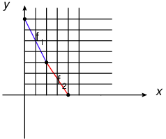
Let’s focus on 3 dimensional singularity from now on, i.e. . Given a Newton non-degenerate singularity, one can define a singularity spectrum using the Newton filtration defined above. For the quasi-homogeneous singularity, the singularity spectrum can be found easily. Let’s take a monomial basis of the Jacobian algebra , the spectrum is given by the following formula
| (81) |
We can denote the spectrum as an ordered set , and rational condition implies , which implies 1010 10 Since is always the generator of with minimal weight, and we have .
For general Newton non-degenerate singularity, it is possible also to find a regular monomial basis of such that the singularity spectrum is given by
| (82) |
Here denotes the exponent of the monomial basis, and denotes the vector . Rational condition implies that . The divisor class group can be expressed [65] as follows
| (83) |
namely we count the number of ones in singularity spectrum .
Remark: These 3d canonical quasi-homogeneous singularity has been used in [1] to study four dimensional SCFT. In that context, the weights with value in singularity spectrum give the mass parameters.
Let’s define a crepant weighting as the weights (here the weighting has positive integral weights on coordinates). We denote all such weighting as . The number of crepant divisors are found as [65]:
| (84) |
where denotes the face of corresponding to .
7 Conclusion
We argue that every 3-fold canonical singularity defines a five dimensional SCFT. We can read off the non-abelian flavor symmetry from the singularity structure, and the Coulomb branch is described by the crepant resolutions of the singularity. For each crepant resolution, one can compute Nef cone which describes a chamber of Coulomb branch. The faces of Nef cone correspond to the locus where an extra massless particle appears. Different resolutions are related by flops, and these Nef cones form a fan which is claimed to be the full Coulomb branch.
We have given a description for the Coulomb branch of several simple theories defined by toric singularity. Detailed computations for prepotential and Coulomb branch structure for other interesting toric theories will appear elsewhere. The non-toric example would be also interesting to study too, i.e. complex cone over Fano orbifolds should be interesting to study.
It would be interesting to study other properties of these theories such as superconformal index and Seiberg-Witten curve for 5d theory on circle.
Acknowledgements
DX would like to thank H.C Kim, P. Jefferson, K. Yonekura for helpful discussions. DX would like to thank Korea Institute for Advanced Study, University of Cincinatti, Aspen center for physics for hospitality during various stages of this work. The work of S.T Yau is supported by NSF grant DMS-1159412, NSF grant PHY- 0937443, and NSF grant DMS-0804454. The work of DX is supported by Center for Mathematical Sciences and Applications at Harvard University, and in part by the Fundamental Laws Initiative of the Center for the Fundamental Laws of Nature, Harvard University.
References
- (1) D. Xie and S.-T. Yau, “4d N=2 SCFT and singularity theory Part I: Classification,” arXiv:1510.01324 [hep-th].
- (2) P. C. Argyres and M. R. Douglas, “New phenomena in SU(3) supersymmetric gauge theory,” Nucl. Phys. B448 (1995) 93–126, arXiv:hep-th/9505062 [hep-th].
- (3) P. C. Argyres, M. R. Plesser, N. Seiberg, and E. Witten, “New N=2 superconformal field theories in four-dimensions,” Nucl. Phys. B461 (1996) 71–84, arXiv:hep-th/9511154 [hep-th].
- (4) S. Gukov, C. Vafa, and E. Witten, “CFT’s from Calabi-Yau four folds,” Nucl. Phys. B584 (2000) 69–108, arXiv:hep-th/9906070 [hep-th]. [Erratum: Nucl. Phys.B608,477(2001)].
- (5) B. Chen, D. Xie, S.-T. Yau, S. S. T. Yau, and H. Zuo, “4d N=2 SCFT and singularity theory Part II: Complete intersection,” arXiv:1604.07843 [hep-th].
- (6) Y. Wang, D. Xie, S. S. T. Yau, and S.-T. Yau, “4d N=2 SCFT from Complete Intersection Singularity,” arXiv:1606.06306 [hep-th].
- (7) N. Seiberg, “Five-dimensional SUSY field theories, nontrivial fixed points and string dynamics,” Phys. Lett. B388 (1996) 753–760, arXiv:hep-th/9608111 [hep-th].
- (8) C. Cordova, T. T. Dumitrescu, and K. Intriligator, “Deformations of Superconformal Theories,” arXiv:1602.01217 [hep-th].
- (9) D. R. Morrison and N. Seiberg, “Extremal transitions and five-dimensional supersymmetric field theories,” Nucl. Phys. B483 (1997) 229–247, arXiv:hep-th/9609070 [hep-th].
- (10) K. A. Intriligator, D. R. Morrison, and N. Seiberg, “Five-dimensional supersymmetric gauge theories and degenerations of Calabi-Yau spaces,” Nucl. Phys. B497 (1997) 56–100, arXiv:hep-th/9702198 [hep-th].
- (11) C.-L. Wang, “On the incompleteness of the weil-petersson metric along degenerations of calabi-yau manifolds,” Mathematical Research Letters 4 (1997) 157–172.
- (12) E. Witten, “Some comments on string dynamics,” in Future perspectives in string theory. Proceedings, Conference, Strings’95, Los Angeles, USA, March 13-18, 1995, pp. 501–523. 1995. arXiv:hep-th/9507121 [hep-th].
- (13) M. Buican, J. Hayling, and C. Papageorgakis, “Aspects of Superconformal Multiplets in ,” arXiv:1606.00810 [hep-th].
- (14) E. Witten, “Phase transitions in M theory and F theory,” Nucl. Phys. B471 (1996) 195–216, arXiv:hep-th/9603150 [hep-th].
- (15) M. R. Douglas, S. H. Katz, and C. Vafa, “Small instantons, Del Pezzo surfaces and type I-prime theory,” Nucl. Phys. B497 (1997) 155–172, arXiv:hep-th/9609071 [hep-th].
- (16) N. C. Leung and C. Vafa, “Branes and toric geometry,” Adv. Theor. Math. Phys. 2 (1998) 91–118, arXiv:hep-th/9711013 [hep-th].
- (17) S. Katz, P. Mayr, and C. Vafa, “Mirror symmetry and exact solution of 4-D N=2 gauge theories: 1.,” Adv. Theor. Math. Phys. 1 (1998) 53–114, arXiv:hep-th/9706110 [hep-th].
- (18) O. Aharony, A. Hanany, and B. Kol, “Webs of (p,q) five-branes, five-dimensional field theories and grid diagrams,” JHEP 01 (1998) 002, arXiv:hep-th/9710116 [hep-th].
- (19) A. Iqbal and C. Vafa, “BPS Degeneracies and Superconformal Index in Diverse Dimensions,” Phys. Rev. D90 (2014) no. 10, 105031, arXiv:1210.3605 [hep-th].
- (20) H.-C. Kim, J. Kim, and S. Kim, “Instantons on the 5-sphere and M5-branes,” arXiv:1211.0144 [hep-th].
- (21) B. Assel, J. Estes, and M. Yamazaki, “Wilson Loops in 5d N=1 SCFTs and AdS/CFT,” Annales Henri Poincare 15 (2014) 589–632, arXiv:1212.1202 [hep-th].
- (22) D. Rodríguez-Gómez and G. Zafrir, “On the 5d instanton index as a Hilbert series,” Nucl. Phys. B878 (2014) 1–11, arXiv:1305.5684 [hep-th].
- (23) O. Bergman, D. Rodríguez-Gómez, and G. Zafrir, “5d superconformal indices at large N and holography,” JHEP 08 (2013) 081, arXiv:1305.6870 [hep-th].
- (24) H.-C. Kim, S. Kim, S.-S. Kim, and K. Lee, “The general M5-brane superconformal index,” arXiv:1307.7660 [hep-th].
- (25) L. Bao, V. Mitev, E. Pomoni, M. Taki, and F. Yagi, “Non-Lagrangian Theories from Brane Junctions,” JHEP 01 (2014) 175, arXiv:1310.3841 [hep-th].
- (26) O. Bergman, D. Rodríguez-Gómez, and G. Zafrir, “Discrete and the 5d superconformal index,” JHEP 01 (2014) 079, arXiv:1310.2150 [hep-th].
- (27) H. Hayashi, H.-C. Kim, and T. Nishinaka, “Topological strings and 5d partition functions,” JHEP 06 (2014) 014, arXiv:1310.3854 [hep-th].
- (28) M. Taki, “Notes on Enhancement of Flavor Symmetry and 5d Superconformal Index,” arXiv:1310.7509 [hep-th].
- (29) O. Bergman, D. Rodríguez-Gómez, and G. Zafrir, “5-Brane Webs, Symmetry Enhancement, and Duality in 5d Supersymmetric Gauge Theory,” JHEP 03 (2014) 112, arXiv:1311.4199 [hep-th].
- (30) M. Taki, “Seiberg Duality, 5d SCFTs and Nekrasov Partition Functions,” arXiv:1401.7200 [hep-th].
- (31) C. Hwang, J. Kim, S. Kim, and J. Park, “General instanton counting and 5d SCFT,” JHEP 07 (2015) 063, arXiv:1406.6793 [hep-th]. [Addendum: JHEP04,094(2016)].
- (32) G. Zafrir, “Duality and enhancement of symmetry in 5d gauge theories,” JHEP 12 (2014) 116, arXiv:1408.4040 [hep-th].
- (33) M. Esole, S.-H. Shao, and S.-T. Yau, “Singularities and Gauge Theory Phases,” Adv. Theor. Math. Phys. 19 (2015) 1183–1247, arXiv:1402.6331 [hep-th].
- (34) M. Esole, S.-H. Shao, and S.-T. Yau, “Singularities and Gauge Theory Phases II,” Adv. Theor. Math. Phys. 20 (2016) 683–749, arXiv:1407.1867 [hep-th].
- (35) H. Hayashi and G. Zoccarato, “Exact partition functions of Higgsed 5d theories,” JHEP 01 (2015) 093, arXiv:1409.0571 [hep-th].
- (36) O. Bergman and G. Zafrir, “Lifting 4d dualities to 5d,” JHEP 04 (2015) 141, arXiv:1410.2806 [hep-th].
- (37) V. Mitev, E. Pomoni, M. Taki, and F. Yagi, “Fiber-Base Duality and Global Symmetry Enhancement,” JHEP 04 (2015) 052, arXiv:1411.2450 [hep-th].
- (38) D. Gaiotto and H.-C. Kim, “Surface defects and instanton partition functions,” JHEP 10 (2016) 012, arXiv:1412.2781 [hep-th].
- (39) N. Lambert, C. Papageorgakis, and M. Schmidt-Sommerfeld, “Instanton Operators in Five-Dimensional Gauge Theories,” JHEP 03 (2015) 019, arXiv:1412.2789 [hep-th].
- (40) Y. Tachikawa, “Instanton operators and symmetry enhancement in 5d supersymmetric gauge theories,” PTEP 2015 (2015) no. 4, 043B06, arXiv:1501.01031 [hep-th].
- (41) G. Zafrir, “Instanton operators and symmetry enhancement in 5d supersymmetric USp, SO and exceptional gauge theories,” JHEP 07 (2015) 087, arXiv:1503.08136 [hep-th].
- (42) K. Yonekura, “Instanton operators and symmetry enhancement in 5d supersymmetric quiver gauge theories,” JHEP 07 (2015) 167, arXiv:1505.04743 [hep-th].
- (43) H. Hayashi and G. Zoccarato, “Topological vertex for Higgsed 5d TN theories,” JHEP 09 (2015) 023, arXiv:1505.00260 [hep-th].
- (44) S.-S. Kim, M. Taki, and F. Yagi, “Tao Probing the End of the World,” PTEP 2015 (2015) no. 8, 083B02, arXiv:1504.03672 [hep-th].
- (45) G. Zafrir, “Brane webs and -planes,” JHEP 03 (2016) 109, arXiv:1512.08114 [hep-th].
- (46) O. Bergman and G. Zafrir, “5d fixed points from brane webs and O7-planes,” JHEP 12 (2015) 163, arXiv:1507.03860 [hep-th].
- (47) D. Gaiotto and H.-C. Kim, “Duality walls and defects in 5d N=1 theories,” arXiv:1506.03871 [hep-th].
- (48) O. Bergman and D. Rodriguez-Gomez, “A Note on Instanton Operators, Instanton Particles, and Supersymmetry,” JHEP 05 (2016) 068, arXiv:1601.00752 [hep-th].
- (49) J. Qiu and M. Zabzine, “Review of localization for 5d supersymmetric gauge theories,” 2016. arXiv:1608.02966 [hep-th]. http://inspirehep.net/record/1480393/files/arXiv:1608.02966.pdf.
- (50) C.-M. Chang, O. Ganor, and J. Oh, “An index for ray operators in 5d SCFTs,” JHEP 02 (2017) 018, arXiv:1608.06284 [hep-th].
- (51) E. D’Hoker, M. Gutperle, and C. F. Uhlemann, “Holographic duals for five-dimensional superconformal quantum field theories,” Phys. Rev. Lett. 118 (2017) no. 10, 101601, arXiv:1611.09411 [hep-th].
- (52) E. D’Hoker, M. Gutperle, and C. F. Uhlemann, “Warped in Type IIB supergravity II: Global solutions and five-brane webs,” arXiv:1703.08186 [hep-th].
- (53) M. Esole, P. Jefferson, and M. J. Kang, “Euler Characteristics of Crepant Resolutions of Weierstrass Models,” arXiv:1703.00905 [math.AG].
- (54) H. Hayashi and K. Ohmori, “5d/6d DE instantons from trivalent gluing of web diagrams,” arXiv:1702.07263 [hep-th].
- (55) M. Reid, Canonical 3-folds. University of WArwick, 1979.
- (56) M. Reid, “Minimal models of canonical 3-folds,” Adv. Stud. Pure Math 1 (1983) 131–180.
- (57) M. Reid, “Young personÕs guide to canonical singularities,” Algebraic geometry, Bowdoin 46 (1985) 345–414.
- (58) S. Mori, “On 3-dimensional terminal singularities,” Nagoya Mathematical Journal 98 (1985) 43–66.
- (59) J. Kollár and N. I. Shepherd-Barron, “Threefolds and deformations of surface singularities,” Inventiones mathematicae 91 (1988) no. 2, 299–338.
- (60) D. A. Cox, J. B. Little, and H. K. Schenck, Toric varieties. American Mathematical Soc., 2011.
- (61) S. Rabinowitz, “A census of convex lattice polygons with at most one interior lattice point,” Ars Combin 28 (1989) 83–96.
- (62) X. Wei and R. Ding, “Lattice polygons with two interior lattice points,” Mathematical Notes 91 (2012) no. 5-6, 868–877.
- (63) S. S.-T. Yau and Y. Yu, Gorenstein quotient singularities in dimension three, vol. 505. American Mathematical Soc., 1993.
- (64) S.-S. Roan, “Minimal resolutions of gorenstein orbifolds in dimension three,” Topology 35 (1996) no. 2, 489–508.
- (65) M. CAIBAR, “On the divisor class group of 3-fold singularities,” International Journal of Mathematics 14 (2003) no. 01, 105–117.
- (66) H. Flenner, “Divisorenklassengruppen quasihomogener singularitäten.,” Journal für die reine und angewandte Mathematik 328 (1981) 128–160.