跳到论文正文
W Papers独立论文阅读器 arXiv:1704.00666 论文正文 计算阅读时间 · 0%
引用这篇论文根据当前论文元数据生成,正式投稿前建议核对。


License: arXiv.org perpetual non-exclusive license
arXiv:1704.00666v3 [stat.ME] 15 Jul 2022

Causal inference with observational studies trimmed by the estimated propensity scores

Shu Yang ††thanks: Department of Statistics, North Carolina State University, Raleigh, North Carolina 27695, U.S.A.    Peng Ding ††thanks: Department of Statistics, University of California, Berkeley, California 94720, U.S.A.
Abstract

Causal inference with observational studies often relies on the assumptions of unconfoundedness and overlap of covariate distributions in different treatment groups. The overlap assumption is violated when some units have propensity scores close to zero or one, and therefore both theoretical and practical researchers suggest dropping units with extreme estimated propensity scores. We advance the literature in three directions. First, we clarify a conceptual issue of sample trimming by defining causal parameters based on a target population without extreme propensity score. Second, we propose a procedure of smooth weighting, which approximates the existing sample trimming but has better asymptotic properties. The new weighting estimator is asymptotically linear and the bootstrap can be used to construct confidence intervals. Third, we extend the theory to the average treatment effect on the treated, suggesting trimming samples with estimated propensity scores close to one.

Some key words: Bootstrap; Lack of overlap; Non-smoothness; Potential outcome; Unconfoundedness.

1 Introduction

Under the potential outcomes framework (Rubin, 1974), causal effects are comparisons of the potential outcomes corresponding to different treatments. There is an extensive literature on estimating average treatment effects based on the assumption of unconfoundedness and sufficient overlap in the covariate distributions (Rosenbaum and Rubin, 1983; Imbens and Rubin, 2015). Unfortunately, in many applications it is common to have limited overlap in covariates between the treatment and control groups, i.e., there are regions of the covariate space with low probability of receiving treatment or control. Lack of overlap affects the credibility of all methods attempting to estimate causal effects for the common population. A consequence in weighting (Rosenbaum and Rubin, 1983; Imbens and Rubin, 2015) is that extreme propensity scores induce substantively large weights, which can result in a large variance and poor finite sample properties (Kang and Schafer, 2007; Khan and Tamer, 2010). In this case, it is desirable to modify the estimand to averaging only over the part of the covariate space with all treatment probabilities away from zero. For example, Crump et al. (2009) suggested dropping subjects from the analysis with estimated propensity score close to zero and one, which generally alters the estimand by changing the reference population (Li et al., 2016). In the current practice, researchers often first trim the samples based on the estimated propensity scores, and then characterize the target population and estimand based on the sample estimates. This ad hoc definition of the treatment effect is problematic, because using different samples may change the target estimand.

The objective of this article is to clarify a conceptual issue of sample trimming, which arises frequently in practice, leading to unambiguous definitions of causal parameters based on a well-defined target population. The non-smooth nature of trimming makes inference complicated. Therefore, instead of making binary decisions to include or exclude subjects from analysis, we propose to use a smooth weighting function so that all subjects are weighted continuously. This smooth weighting approximates the existing sample trimming, but allows us to derive the asymptotic properties of the corresponding causal estimators using conventional linearization methods for two-step statistics. We formally show that the new weighting estimator is asymptotically linear and the bootstrap can be used to construct confidence intervals. Moreover, by smoothing the indicator function, the resulting estimators gain precision, as demonstrated in the asymptotic analysis and simulation study. In addition to the average treatment effect, we extend Crump et al. (2009) to develop an optimal rule to select subpopulation for which the average treatment effect on the treated can be estimated most precisely, and establish asymptotic inference when support reduction is based estimated propensity scores.

2 Notation

For each subject ii, the treatment is Ai∈{0,1}A_{i}\in\{0,1\}, where 00 and 11 are labels for control and treatment. There are two potential outcomes, one for treatment and the other for control, denoted by Yi​(1)Y_{i}(1) and Yi​(0)Y_{i}(0), respectively. The observed outcome is Yi=Yi​(Ai)Y_{i}=Y_{i}(A_{i}). Let XiX_{i} be the observed pre-treatment confounders. We assume that {Ai,Xi,Yi​(1),Yi​(0)}i=1N\{A_{i},X_{i},Y_{i}(1),Y_{i}(0)\}_{i=1}^{N} are independent draws from the distribution of {A,X,Y⁡(1),Y⁡(0)}\{A,X,Y(1),Y(0)\}. Given the observed confounders XX, the conditional average causal effect is τ⁡(X)=E⁡{Y⁡(1)−Y⁡(0)∣X}\tau(X)=E\{Y(1)-Y(0)\mid X\}. The average treatment effect is τ=E​{τ⁡(X)}\tau=E\{\tau(X)\}, where the expectation is taken with respect to the whole population. The common assumptions to identify τ\tau are as follows (Rosenbaum and Rubin, 1983).

Assumption 1 (Unconfoundedness)

Y⁡(a)⊥A|XY(a)\bot A\mid X for a=0,1a=0,1.

Assumption 2 (Sufficient overlap)

There exist constants c1c_{1} and c2c_{2} such that with probability 11, 0<c1≤e⁡(X)≤c2<10<c_{1}\leq e(X)\leq c_{2}<1, where e⁡(X)=pr⁡(A=1∣X)e(X)=\mathrm{pr}(A=1\mid X) is the propensity score.

Assumption 3

E​{Y​(a)2}<∞E\{Y(a)^{2}\}<\infty, for a=0,1a=0,1.

In observational studies the propensity score is not known and therefore has to be estimated from data. Following Rosenbaum and Rubin (1983) and most of the empirical literature, we assume that the propensity score is correctly specified by a generalized linear model e⁡(X)=e⁡(X′​θ∗)e(X)=e(X^{\prime}\theta^{*}). Let θ^\hat{\theta} be the maximum likelihood estimator of θ∗\theta^{*}. Our method is also applicable to other asymptotically linear estimators of θ\theta. Then, a simple weighting estimator of τ\tau is N−1​∑i=1Nτ^​(Xi)N^{-1}\sum_{i=1}^{N}\hat{\tau}(X_{i}), where

τ^​(Xi)=Ai​Yie⁡(Xi′​θ^)−(1−Ai)​Yi1−e⁡(Xi′​θ^).\hat{\tau}(X_{i})=\frac{A_{i}Y_{i}}{e(X_{i}^{\prime}\hat{\theta})}-\frac{(1-A_{i})Y_{i}}{1-e(X_{i}^{\prime}\hat{\theta})}. (1)

The augmented weighting estimator (Lunceford and Davidian, 2004; Bang and Robins, 2005) augments the simple weighting estimator by further estimating μ⁡(a,X)=E⁡(Y∣A=a,X)\mu(a,X)=E(Y\mid A=a,X) by μ^​(a,X)\hat{\mu}(a,X), and using N−1​∑i=1Nτ^aug​(Xi),N^{-1}\sum_{i=1}^{N}\hat{\tau}^{\mathrm{aug}}(X_{i}), where

τ^aug​(Xi)=[Ai​Yie⁡(Xi′​θ^)+{1−Aie⁡(Xi′​θ^)}​μ^​(1,Xi)]−[(1−Ai)​Yi1−e⁡(Xi′​θ^)+{1−1−Ai1−e⁡(Xi′​θ^)}​μ^​(0,Xi)].\hat{\tau}^{\mathrm{aug}}(X_{i})=\left[\frac{A_{i}Y_{i}}{e(X_{i}^{\prime}\hat{\theta})}+\left\{1-\frac{A_{i}}{e(X_{i}^{\prime}\hat{\theta})}\right\}\hat{\mu}(1,X_{i})\right]\\ -\left[\frac{(1-A_{i})Y_{i}}{1-e(X_{i}^{\prime}\hat{\theta})}+\left\{1-\frac{1-A_{i}}{1-e(X_{i}^{\prime}\hat{\theta})}\right\}\hat{\mu}(0,X_{i})\right]. (2)

The augmented weighting estimator features a double robustness property in the sense that under Assumptions 1–3, if either e⁡(X)e(X) or μ⁡(a,X)\mu(a,X) is correctly specified, τ^aug\hat{\tau}^{\mathrm{aug}} is consistent for τ\tau.

The weighting estimators suffer from large variability especially when Assumption 2 is violated or close to be violated. In the presence of lack of overlap, define the set with sufficient overlap to be 𝒪={x∣α≤e⁡(x)≤1−α}\mathcal{O}=\{x\mid\alpha\leq e(x)\leq 1-\alpha\}, where α\alpha is a fixed cut-off value, e.g., a rule of thumb is α=0.1\alpha=0.1, as suggested by Crump et al. (2009). The target population is then represented by 𝒪\mathcal{O}, and the estimand of interest becomes τ⁡(𝒪)=E⁡{τ⁡(X)∣X∈𝒪}\tau(\mathcal{O})=E\{\tau(X)\mid X\in\mathcal{O}\}. This estimand does not depend on the sample, which is more straightforward to interpret.

In existing sampling trimming, the inclusion weight is

ω(Xi′θ^)=1{Xi∈𝒪^}=1{α≤e(Xi′θ^)≤1−α},\omega(X_{i}^{\prime}\hat{\theta})=1_{\{X_{i}\in\hat{\mathcal{O}}\}}=1_{\{\alpha\leq e(X_{i}^{\prime}\hat{\theta})\leq 1-\alpha\}}, (3)

where 1{⋅}1_{\{\cdot\}} being the indicator function, and 𝒪^={x∣α≤e⁡(x′​θ^)≤1−α}\hat{\mathcal{O}}=\{x\mid\alpha\leq e(x^{\prime}\hat{\theta})\leq 1-\alpha\} is the trimmed sample based on the estimated propensity scores. The weighting estimators of τ⁡(𝒪)\tau(\mathcal{O}) become

τ^​(θ^)={∑i=1Nω⁡(Xi′​θ^)}−1​∑i=1Nω⁡(Xi′​θ^)​τ^​(Xi),\hat{\tau}(\hat{\theta})=\left\{\sum_{i=1}^{N}\omega(X_{i}^{\prime}\hat{\theta})\right\}^{-1}\sum_{i=1}^{N}\omega(X_{i}^{\prime}\hat{\theta})\hat{\tau}(X_{i}), (4)
τ^aug​(θ^)={∑i=1Nω⁡(Xi′​θ^)}−1​∑i=1Nω⁡(Xi′​θ^)​τ^aug​(Xi),\hat{\tau}^{\mathrm{aug}}(\hat{\theta})=\left\{\sum_{i=1}^{N}\omega(X_{i}^{\prime}\hat{\theta})\right\}^{-1}\sum_{i=1}^{N}\omega(X_{i}^{\prime}\hat{\theta})\hat{\tau}^{\mathrm{aug}}(X_{i}), (5)

where τ^​(Xi)\hat{\tau}(X_{i}) and τ^aug​(Xi)\hat{\tau}^{\mathrm{aug}}(X_{i}) are defined in (1) and (2), respectively. We write τ^=τ^​(θ^)\hat{\tau}=\hat{\tau}(\hat{\theta}) and τ^aug=τ^aug​(θ^)\hat{\tau}^{\mathrm{aug}}=\hat{\tau}^{\mathrm{aug}}(\hat{\theta}) in shorthand.

The main question addressed in this article is how the estimated support affects the inference. To study the asymptotic behaviors of τ^\hat{\tau} and τ^aug\hat{\tau}^{\mathrm{aug}}, we need to take into account of first the sampling variability in θ^\hat{\theta}, which induces variability of the estimated set 𝒪^\hat{\mathcal{O}} and second the sampling variability in τ^\hat{\tau} and τ^aug\hat{\tau}^{\mathrm{aug}}. We can not directly apply conventional asymptotic linearization methods because the weight function (3) is non-smooth. To avoid this difficulty, we consider a smoothed version of the weight function

ωϵ​(Xi′​θ^)=Φϵ​{e⁡(Xi′​θ^)−α}​Φϵ​{1−α−e⁡(Xi′​θ^)},\omega_{\epsilon}(X_{i}^{\prime}\hat{\theta})=\Phi_{\epsilon}\left\{e(X_{i}^{\prime}\hat{\theta})-\alpha\right\}\Phi_{\epsilon}\left\{1-\alpha-e(X_{i}^{\prime}\hat{\theta})\right\}, (6)

where Φϵ​(z)\Phi_{\epsilon}(z) is a normal cumulative distribution with mean zero and variance ϵ\epsilon. The new weight function imposes a soft threshold, instead of a hard threshold which results in weights either zero or one, for the estimated propensity scores close to α\alpha and 1−α1-\alpha. An important issue regarding this weight function is the choice of ϵ\epsilon. As ϵ→0\epsilon\rightarrow 0, the smooth weight function (6) coverages to the indicator weight function (3); see Figure S1 in the Supplementary Material for visualization of the weight functions. Therefore, for small ϵ\epsilon, the behaviors of the estimators (4) and (5) with the smooth weight function (6) are similar to those with the indicator weight function (3). We derive the asymptotic results for the smoothed estimators.

3 Main Results

Based on data {(Ai,Xi)}i=1N\{(A_{i},X_{i})\}_{i=1}^{N}, let the score function and the Fisher information matrix of θ\theta be

S⁡(θ)=1N​∑i=1NXi​Ai−e⁡(Xi′​θ)e⁡(Xi′​θ)​{1−e⁡(Xi′​θ)}​f​(Xi′​θ),ℐθ=E⁡[f​(X′​θ)2e⁡(X′​θ)​{1−e⁡(X′​θ)}​X​X′],S(\theta)=\frac{1}{N}\sum_{i=1}^{N}X_{i}\frac{A_{i}-e(X_{i}^{\prime}\theta)}{e(X_{i}^{\prime}\theta)\{1-e(X_{i}^{\prime}\theta)\}}f(X_{i}^{\prime}\theta),\quad\mathcal{I}_{\theta}=E\left[\frac{f(X^{\prime}\theta)^{2}}{e(X^{\prime}\theta)\{1-e(X^{\prime}\theta)\}}XX^{\prime}\right],

respectively, where f⁡(t)=d​e​(t)/d​tf(t)=\mathrm{d}e(t)/\mathrm{d}t. Because θ^\hat{\theta} is the solution to the score equation S⁡(θ)=0S(\theta)=0, under certain regularity conditions, θ^−θ∗=ℐθ∗−1S(θ∗)+op(N−1/2).\hat{\theta}-\theta^{*}=\mathcal{I}_{\theta^{*}}^{-1}S(\theta^{*})+o_{p}(N^{-1/2}). Let σ2​(a,X)=var⁡(Y∣A=a,X)\sigma^{2}(a,X)=\mathrm{var}(Y\mid A=a,X), for a=0,1a=0,1. Denote τ^ϵ\hat{\tau}_{\epsilon} to be the weighting estimator (4) with the smooth weight function (6), and τϵ=E⁡{ωϵ​(X′​θ∗)​τ​(X)}\tau_{\epsilon}=E\{\omega_{\epsilon}(X^{\prime}\theta^{*})\tau(X)\}.

Theorem 1

Under Assumptions 1 and 3, τ^ϵ\hat{\tau}_{\epsilon} is asymptotically linear. Moreover,

N1/2​(τ^ϵ−τϵ)→𝒩⁡(0,σϵ2+b1,ϵ′​ℐθ∗−1​b1,ϵ−b2,ϵ′​ℐθ∗−1​b2,ϵ),N^{1/2}(\hat{\tau}_{\epsilon}-\tau_{\epsilon})\rightarrow\mathcal{N}\left(0,\sigma_{\epsilon}^{2}+b_{1,\epsilon}^{\prime}\mathcal{I}_{\theta^{*}}^{-1}b_{1,\epsilon}-b_{2,\epsilon}^{\prime}\mathcal{I}_{\theta^{*}}^{-1}b_{2,\epsilon}\right),

in distribution, as N→∞N\rightarrow\infty, where

b1,ϵ=E⁡{∂∂θ​[ωϵ​(X′​θ∗)E⁡{ωϵ​(X′​θ∗)}]​τ​(X)},b_{1,\epsilon}=E\left\{\frac{\partial}{\partial\theta}\left[\frac{\omega_{\epsilon}(X^{\prime}\theta^{*})}{E\{\omega_{\epsilon}(X^{\prime}\theta^{*})\}}\right]\tau(X)\right\}, (7)
b2,ϵ=1E⁡{ωϵ​(X′​θ∗)}​E​{ωϵ​(X′​θ∗)​f​(X′​θ∗)​[E​{X​μ​(1,X)∣e⁡(X)}e⁡(X)+E​{X​μ​(0,X)∣e⁡(X)}1−e⁡(X)]},b_{2,\epsilon}=\frac{1}{E\{\omega_{\epsilon}(X^{\prime}\theta^{*})\}}E\left\{\omega_{\epsilon}(X^{\prime}\theta^{*})f(X^{\prime}\theta^{*})\left[\frac{E\{X\mu(1,X)\mid e(X)\}}{e(X)}+\frac{E\{X\mu(0,X)\mid e(X)\}}{1-e(X)}\right]\right\},
σϵ2\displaystyle\sigma_{\epsilon}^{2} =\displaystyle= 1E​{ωϵ​(X′​θ∗)}2​var​{ωϵ​(X′​θ∗)​τ​(X)}\displaystyle\frac{1}{E\{\omega_{\epsilon}(X^{\prime}\theta^{*})\}^{2}}\mathrm{var}\left\{\omega_{\epsilon}(X^{\prime}\theta^{*})\tau(X)\right\}
+1E​{ωϵ​(X′​θ∗)}2​E​{ωϵ​(X′​θ∗)2​[{1−e⁡(X)e⁡(X)}1/2​μ​(1,X)+{e⁡(X)1−e⁡(X)}1/2​μ​(0,X)]2}\displaystyle+\frac{1}{E\{\omega_{\epsilon}(X^{\prime}\theta^{*})\}^{2}}E\left\{\omega_{\epsilon}(X^{\prime}\theta^{*})^{2}\left[\left\{\frac{1-e(X)}{e(X)}\right\}^{1/2}\mu(1,X)+\left\{\frac{e(X)}{1-e(X)}\right\}^{1/2}\mu(0,X)\right]^{2}\right\}
+1E​{ωϵ​(X′​θ∗)}2​E​[ωϵ​(X′​θ∗)2​{σ2​(1,X)e⁡(X)+σ2​(0,X)1−e⁡(X)}].\displaystyle+\frac{1}{E\{\omega_{\epsilon}(X^{\prime}\theta^{*})\}^{2}}E\left[\omega_{\epsilon}(X^{\prime}\theta^{*})^{2}\left\{\frac{\sigma^{2}(1,X)}{e(X)}+\frac{\sigma^{2}(0,X)}{1-e(X)}\right\}\right].
Remark 1

The term b1,ϵ′​ℐθ∗−1​b1,ϵb_{1,\epsilon}^{\prime}\mathcal{I}_{\theta^{*}}^{-1}b_{1,\epsilon} is the increased variability due to estimating the support. We now show that this term is close to zero for small ϵ\epsilon. We note

∂∂θ​[ωϵ​(X′​θ∗)E⁡{ωϵ​(X′​θ∗)}]=ω˙ϵ​(X′​θ∗)​E​{ωϵ​(X′​θ∗)}−E⁡{ω˙ϵ​(X′​θ∗)}​ωϵ​(X′​θ∗)[E⁡{ωϵ​(X′​θ∗)}]2,\frac{\partial}{\partial\theta}\left[\frac{\omega_{\epsilon}(X^{\prime}\theta^{*})}{E\{\omega_{\epsilon}(X^{\prime}\theta^{*})\}}\right]=\frac{\dot{\omega}_{\epsilon}(X^{\prime}\theta^{*})E\{\omega_{\epsilon}(X^{\prime}\theta^{*})\}-E\{\dot{\omega}_{\epsilon}(X^{\prime}\theta^{*})\}\omega_{\epsilon}(X^{\prime}\theta^{*})}{[E\{\omega_{\epsilon}(X^{\prime}\theta^{*})\}]^{2}}, (8)

where

ω˙ϵ​(X′​θ∗)\displaystyle\dot{\omega}_{\epsilon}(X^{\prime}\theta^{*}) =\displaystyle= ∂∂θ​[Φϵ​{e⁡(X′​θ∗)−α}​Φϵ​{1−α−e⁡(X′​θ∗)}]\displaystyle\frac{\partial}{\partial\theta}\left[\Phi_{\epsilon}\left\{e(X^{\prime}\theta^{*})-\alpha\right\}\Phi_{\epsilon}\left\{1-\alpha-e(X^{\prime}\theta^{*})\right\}\right]
=\displaystyle= ϕϵ​{e⁡(X′​θ∗)−α}​Φϵ​{1−α−e⁡(X′​θ∗)}​f​(X′​θ∗)​X\displaystyle\phi_{\epsilon}\left\{e(X^{\prime}\theta^{*})-\alpha\right\}\Phi_{\epsilon}\left\{1-\alpha-e(X^{\prime}\theta^{*})\right\}f(X^{\prime}\theta^{*})X
−Φϵ​{e⁡(X′​θ∗)−α}​ϕϵ​{1−α−e⁡(X′​θ∗)}​f​(X′​θ∗)​X,\displaystyle-\Phi_{\epsilon}\left\{e(X^{\prime}\theta^{*})-\alpha\right\}\phi_{\epsilon}\left\{1-\alpha-e(X^{\prime}\theta^{*})\right\}f(X^{\prime}\theta^{*})X,

and ϕϵ​(x)=d​Φϵ​(x)/d​x\phi_{\epsilon}(x)=\mathrm{d}\Phi_{\epsilon}(x)/\mathrm{d}x. As ϵ→0\epsilon\rightarrow 0, because ϕϵ​(x)→0\phi_{\epsilon}(x)\rightarrow 0, the right hand side of (8), and therefore b1,ϵb_{1,\epsilon}, go to zero. The increased variability due to the estimated support is close to zero with small ϵ\epsilon.

Remark 2

The term −b2,ϵ′​ℐθ−1​b2,ϵ-b_{2,\epsilon}^{\prime}\mathcal{I}_{\theta}^{-1}b_{2,\epsilon} implies that the estimated propensity score increases the precision of the simple weighting estimator of τ\tau based on the true propensity score, which has been demonstrated in the missing data and causal literature; see, e.g., Rubin and Thomas (1992) and Abadie and Imbens (2016).

Remark 3

Assuming that τ⁡(X)\tau(X) is integrable, by the Dominated Convergence Theorem, τϵ\tau_{\epsilon} converges to τ⁡(𝒪)\tau(\mathcal{O}) as ϵ→0\epsilon\rightarrow 0. This implies that our inference based on τ^ϵ\hat{\tau}_{\epsilon}, by choosing a small ϵ\epsilon, can be drawn for the target population represented by 𝒪\mathcal{O}.

Let τ^ϵaug\hat{\tau}_{\epsilon}^{\mathrm{aug}} be the weighting estimator (5) with the smooth weight function (6).

Theorem 2

Under Assumptions 1 and 3, τ^ϵaug\hat{\tau}_{\epsilon}^{\mathrm{aug}} is asymptotically linear. Moreover,

N1/2​(τ^ϵaug−τϵ)→𝒩⁡{0,σ~ϵ2+b1​ϵ′​ℐθ∗​b1​ϵ+(C0+C1)′​ℐθ∗​(C0+C1)+B~′​(C0−C1)},N^{1/2}(\hat{\tau}_{\epsilon}^{\mathrm{aug}}-\tau_{\epsilon})\rightarrow\mathcal{N}\left\{0,\tilde{\sigma}_{\epsilon}^{2}+b_{1\epsilon}^{\prime}\mathcal{I}_{\theta^{*}}b_{1\epsilon}+(C_{0}+C_{1})^{\prime}\mathcal{I}_{\theta^{*}}(C_{0}+C_{1})+\tilde{B}^{\prime}(C_{0}-C_{1})\right\},

in distribution, as N→∞N\rightarrow\infty, where b1,ϵb_{1,\epsilon} is defined in (7),

σ~ϵ2\displaystyle\tilde{\sigma}_{\epsilon}^{2} =\displaystyle= 1E​{ωϵ​(X′​θ∗)}2​var​{ωϵ​(X′​θ∗)​τ​(X)}\displaystyle\frac{1}{E\{\omega_{\epsilon}(X^{\prime}\theta^{*})\}^{2}}\mathrm{var}\left\{\omega_{\epsilon}(X^{\prime}\theta^{*})\tau(X)\right\}
+1E​{ωϵ​(X′​θ∗)}2​E​[ωϵ​(X′​θ∗)2​{σ2​(1,X)e⁡(X)+σ2​(0,X)1−e⁡(X)}],\displaystyle+\frac{1}{E\{\omega_{\epsilon}(X^{\prime}\theta^{*})\}^{2}}E\left[\omega_{\epsilon}(X^{\prime}\theta^{*})^{2}\left\{\frac{\sigma^{2}(1,X)}{e(X)}+\frac{\sigma^{2}(0,X)}{1-e(X)}\right\}\right],
C0=E⁡{X​ωϵ​(X′​θ∗)​f​(X′​θ∗)​μ~​(0,X)−μ​(0,X)1−e⁡(X)},C_{0}=E\left\{X\omega_{\epsilon}(X^{\prime}\theta^{*})f(X^{\prime}\theta^{*})\frac{\tilde{\mu}(0,X)-\mu(0,X)}{1-e(X)}\right\},
C1=E⁡{X​ωϵ​(X′​θ∗)​f​(X′​θ∗)​μ~​(1,X)−μ​(1,X)e⁡(X)},C_{1}=E\left\{X\omega_{\epsilon}(X^{\prime}\theta^{*})f(X^{\prime}\theta^{*})\frac{\tilde{\mu}(1,X)-\mu(1,X)}{e(X)}\right\},

with μ^​(a,X)→μ~​(a,X)\hat{\mu}(a,X)\rightarrow\tilde{\mu}(a,X) in probability, for a=0,1a=0,1, and B~=b1,ϵ−C0−C1\tilde{B}=b_{1,\epsilon}-C_{0}-C_{1}.

Remark 4

The term b1,ϵ′​ℐθ∗−1​b1,ϵb_{1,\epsilon}^{\prime}\mathcal{I}_{\theta^{*}}^{-1}b_{1,\epsilon} can be made small by choosing a small ϵ\epsilon, as shown in Remark 1. If the outcome model is correctly specified, μ~​(a,X)=μ​(a,X)\tilde{\mu}(a,X)=\mu(a,X), and consequently, C0=C1=0C_{0}=C_{1}=0. The asymptotic variance of τ^ϵaug\hat{\tau}_{\epsilon}^{\mathrm{aug}} reduces to σ~ϵ2+b1​ϵ′​ℐθ∗​b1​ϵ\tilde{\sigma}_{\epsilon}^{2}+b_{1\epsilon}^{\prime}\mathcal{I}_{\theta^{*}}b_{1\epsilon}, which is more efficient than τ^ϵ\hat{\tau}_{\epsilon}. Intuitively, this occurs because by regressing YY on XX and AA, we are essentially using the residual as the new outcome, which in general has smaller variance than YY.

Remark 5

Because τ^ϵ\hat{\tau}_{\epsilon} and τ^ϵaug\hat{\tau}_{\epsilon}^{\mathrm{aug}} are asymptotically linear, the bootstrap can be used to estimate the variances of τ^ϵ\hat{\tau}_{\epsilon} and τ^ϵaug\hat{\tau}_{\epsilon}^{\mathrm{aug}} (Shao and Tu, 2012). Let 𝒮={x∣e(x′θ∗)=α\mathcal{S}=\{x\mid e(x^{\prime}\theta^{*})=\alpha or 1−α}1-\alpha\}. If pr⁡(X∈𝒮)=0\mathrm{pr}(X\in\mathcal{S})=0, we conjecture that the bootstrap works for the weighting estimator with the indicator function. This is demonstrated in the simulation study.

4 Average treatment effect on the treated

Another estimand of interest is the average treatment effect for the treated τATT=E⁡{Y⁡(1)−Y⁡(0)∣A=1}=E⁡{τ⁡(X)∣A=1}\tau_{\mathrm{ATT}}=E\{Y(1)-Y(0)\mid A=1\}=E\{\tau(X)\mid A=1\} (Rubin, 1977; Hirano and Imbens, 2001). The outcome distribution for the treated is empirically identifiable E⁡{Y⁡(1)∣A=1}=E⁡(Y∣A=1)E\{Y(1)\mid A=1\}=E(Y\mid A=1), and therefore Assumptions 1 and 2 can be weakened (Heckman et al., 1997).

Assumption 4

Y⁡(0)⊥A|XY(0)\bot A\mid X.

Assumption 5

There exists a constant c2c_{2} such that with probability 11, e⁡(X)≤c2<1e(X)\leq c_{2}<1.

A simple weighting estimator of τATT\tau_{\mathrm{ATT}} (Hirano et al., 2003) is

τ^ATT=∑i=1NAi​Yi∑i=1Ne⁡(Xi′​θ^)−∑i=1N(1−Ai)​Yi​e​(Xi′​θ^)/{1−e⁡(Xi′​θ^)}∑i=1Ne⁡(Xi′​θ^)=∑i=1Ne⁡(Xi′​θ^)​τ^​(Xi)∑i=1Ne⁡(Xi′​θ^).\hat{\tau}_{\mathrm{ATT}}=\frac{\sum_{i=1}^{N}A_{i}Y_{i}}{\sum_{i=1}^{N}e(X_{i}^{\prime}\hat{\theta})}-\frac{\sum_{i=1}^{N}(1-A_{i})Y_{i}e(X_{i}^{\prime}\hat{\theta})/\{1-e(X_{i}^{\prime}\hat{\theta})\}}{\sum_{i=1}^{N}e(X_{i}^{\prime}\hat{\theta})}=\frac{\sum_{i=1}^{N}e(X_{i}^{\prime}\hat{\theta})\hat{\tau}(X_{i})}{\sum_{i=1}^{N}e(X_{i}^{\prime}\hat{\theta})}. (9)

By the above expression, τ^ATT\hat{\tau}_{\mathrm{ATT}} is a special case of the weighting estimator (4) by choosing ω⁡(Xi′​θ^)=e⁡(Xi′​θ^)\omega(X_{i}^{\prime}\hat{\theta})=e(X_{i}^{\prime}\hat{\theta}). Analogously, we propose the augmented weighting estimator of τATT\tau_{\mathrm{ATT}},

τ^ATTaug\displaystyle\hat{\tau}_{\mathrm{ATT}}^{\mathrm{aug}} =\displaystyle= ∑i=1Ne⁡(Xi′​θ^)​τ^aug​(Xi)∑i=1Ne⁡(Xi′​θ^).\displaystyle\frac{\sum_{i=1}^{N}e(X_{i}^{\prime}\hat{\theta})\hat{\tau}^{\mathrm{aug}}(X_{i})}{\sum_{i=1}^{N}e(X_{i}^{\prime}\hat{\theta})}. (10)

There is a limited literature dealing with the lack of overlap for τATT\tau_{\mathrm{ATT}} when Assumption 5 may not hold. Similar to Crump et al. (2009), assuming that σ2​(1,X)=σ2​(0,X)\sigma^{2}(1,X)=\sigma^{2}(0,X), we can show that the optimal overlap for estimating τATT\tau_{\mathrm{ATT}} is of the form 𝒪={x∣1−e⁡(x)≥α}\mathcal{O}=\{x\mid 1-e(x)\geq\alpha\} for some α\alpha, for which the estimators have smallest asymptotic variance. Intuitively, for the treated subjects with e⁡(X)e(X) close to one, there are no similar subjects in the control group that can provide adequate information to infer Y⁡(0)Y(0) for these treated subjects. Statistically, the control subjects with e⁡(X)e(X) close to one contribute to large weights. Therefore, it is reasonable to drop these subjects with e⁡(X)e(X) close to one. By restricting the focus to the optimal set, the estimand of interest becomes τATT(𝒪)=E{τ(X)∣A=1,X∈𝒪}\tau_{\mathrm{ATT}}(\mathcal{O})=E\{\tau(X)\mid A=1,X\in\mathcal{O}\}, for which we propose two estimators with smooth inclusion weights as

τ^ATT,ϵ\displaystyle\hat{\tau}_{\mathrm{ATT},\epsilon} =\displaystyle= ∑i=1NΦϵ​{1−α−e⁡(Xi′​θ^)}​e​(Xi′​θ^)​τ^​(Xi)∑i=1NΦϵ​{1−α−e⁡(Xi′​θ^)}​e​(Xi′​θ^),\displaystyle\frac{\sum_{i=1}^{N}\Phi_{\epsilon}\{1-\alpha-e(X_{i}^{\prime}\hat{\theta})\}e(X_{i}^{\prime}\hat{\theta})\hat{\tau}(X_{i})}{\sum_{i=1}^{N}\Phi_{\epsilon}\{1-\alpha-e(X_{i}^{\prime}\hat{\theta})\}e(X_{i}^{\prime}\hat{\theta})},
τ^ATT,ϵaug\displaystyle\hat{\tau}_{\mathrm{ATT},\epsilon}^{\mathrm{aug}} =\displaystyle= ∑i=1NΦϵ​{1−α−e⁡(Xi′​θ^)}​e​(Xi′​θ^)​τ^aug​(Xi)∑i=1NΦϵ​{1−α−e⁡(Xi′​θ^)}​e​(Xi′​θ^).\displaystyle\frac{\sum_{i=1}^{N}\Phi_{\epsilon}\{1-\alpha-e(X_{i}^{\prime}\hat{\theta})\}e(X_{i}^{\prime}\hat{\theta})\hat{\tau}^{\mathrm{aug}}(X_{i})}{\sum_{i=1}^{N}\Phi_{\epsilon}\{1-\alpha-e(X_{i}^{\prime}\hat{\theta})\}e(X_{i}^{\prime}\hat{\theta})}.

The asymptotic properties can be derived similarly as in Theorems 1 and 2 by recognizing ωϵ​(X′​θ^)=Φϵ​{1−α−e⁡(Xi′​θ^)}​e​(Xi′​θ^)\omega_{\epsilon}(X^{\prime}\hat{\theta})=\Phi_{\epsilon}\{1-\alpha-e(X_{i}^{\prime}\hat{\theta})\}e(X_{i}^{\prime}\hat{\theta}) for τ^ATT,ϵ\hat{\tau}_{\mathrm{ATT},\epsilon} and τ^ATT,ϵaug\hat{\tau}_{\mathrm{ATT},\epsilon}^{\mathrm{aug}}. In particular, the asymptotic linearity enables the bootstrap for inference. See the Supplementary Material for details. Similar discussion applies to estimating the average treatment effect on the control.

5 Simulation study

We assess the performance of the new weighting estimators of the average treatment effect over a target population. We consider six covariates XjX_{j} (j=1,…,6)(j=1,\ldots,6), where X1X_{1}, X2X_{2}, and X3X_{3} are multivariate normal with means (0,0,0)(0,0,0), variances (2,1,1)(2,1,1) and covariances (1,−1,−0.5)(1,-1,-0.5), X4∼Uniform⁡[−3,3]X_{4}\sim\mathrm{Uniform}[-3,3], X5∼χ12X_{5}\sim\chi_{1}^{2}, and X6∼Bernoulli⁡(0.5)X_{6}\sim\mathrm{Bernoulli}(0.5). Let X=(X1,X2,X3,X4,X5,X6)′X=(X_{1},X_{2},X_{3},X_{4},X_{5},X_{6})^{\prime} be the 6-component vector of covariates. The treatment indicator AA is generated from a Bernoulli distribution with probability e⁡(X)e(X). We consider four propensity score deigns:

(P1)

e⁡(X)=logit⁡{0.1×(X1+X2+X3+X4+X5+X6)}e(X)=\mathrm{logit}\{0.1\times(X_{1}+X_{2}+X_{3}+X_{4}+X_{5}+X_{6})\}.

(P2)

e⁡(X)=logit⁡{0.8×(X1+X2+X3+X4+X5+X6)}e(X)=\mathrm{logit}\{0.8\times(X_{1}+X_{2}+X_{3}+X_{4}+X_{5}+X_{6})\}.

(P3)

e⁡(X)=logit⁡{0.1×(X1+X22+X32+X4+X5+X6)}e(X)=\mathrm{logit}\{0.1\times(X_{1}+X_{2}^{2}+X_{3}^{2}+X_{4}+X_{5}+X_{6})\}.

(P4)

e⁡(X)=logit⁡{0.8×(X1+X22+X32+X4+X5+X6)}e(X)=\mathrm{logit}\{0.8\times(X_{1}+X_{2}^{2}+X_{3}^{2}+X_{4}+X_{5}+X_{6})\}.

(P1) and (P3) represent week separations of propensity score distributions between the treatment and control groups; (P2) and (P4) represent strong separations. See Figure S.2 in the Supplementary Material for visualization of propensity score distributions. We consider two outcome designs:

(O1)

Y⁡(a)=a⁡(X1+X2+X3−X4+X5+X6)+ηY(a)=a(X_{1}+X_{2}+X_{3}-X_{4}+X_{5}+X_{6})+\eta, with η∼𝒩⁡(0,1)\eta\sim\mathcal{N}(0,1), for a=0,1a=0,1.

(O2)

Y⁡(a)=a​(X1+X2+X3)2+ηY(a)=a(X_{1}+X_{2}+X_{3})^{2}+\eta, with η∼𝒩⁡(0,1)\eta\sim\mathcal{N}(0,1), for a=0,1a=0,1.

(O1) is a linear case, and (O2) is a non-linear case. The sample size is set to be N=500N=500. The target population is represented by 𝒪={x∣α<e⁡(x)<1−α}\mathcal{O}=\{x\mid\alpha<e(x)<1-\alpha\} with α=0.1\alpha=0.1, and the estimand of interest τ⁡(𝒪)\tau(\mathcal{O}) is the average treatment effect over the target population.

We consider the weighting estimators with indicator weight function and smooth weight function, and τ(𝒪)=(∑i=1N1{Xi∈𝒪})−1∑i=1N1{Xi∈𝒪}{Yi(1)−Yi(0)}\tau(\mathcal{O})=(\sum_{i=1}^{N}1_{\{X_{i}\in\mathcal{O}\}})^{-1}\sum_{i=1}^{N}1_{\{X_{i}\in\mathcal{O}\}}\{Y_{i}(1)-Y_{i}(0)\} for benchmark comparison. The propensity scores are estimated by a logistic regression model with linear predictors XX. Therefore, the propensity score model is correctly specified under (P1) and (P2), but it is misspecified under (P3) and (P4). For the augmented weighting estimators, μ⁡(a,X)\mu(a,X) is estimated by a simple regression of YY on XX, separately for A=aA=a (a=0,1a=0,1). Therefore, the outcome regression model is correctly specified under (O1) but misspecified under (O2).

Table 1: Results: mean, variance (var), and variance estimate (ve) by 100100 bootstrapping under eight combinations of outcome design and propensity score design: c indicates the corresponding model is correctly specified , and w indicates the corresponding model is incorrectly specified
Scenario i (OD1c, PSD1c) ii (OD1c, PSD2c) iii (OD1c, PSD3w) iv (OD1c, PSD4w)
ϵ\epsilon mean var ve mean var ve mean var ve mean var ve
τ⁡(𝒪)\tau(\mathcal{O}) 1.46 1.33 1.44 1.37
τ^​(θ^)\hat{\tau}(\hat{\theta}) – 1.45 0.0341 0.0336 1.33 0.0471 0.0518 1.48 0.0285 0.0282 1.45 0.0399 0.0405
τ^aug​(θ^)\hat{\tau}^{\mathrm{aug}}(\hat{\theta}) – 1.46 0.0282 0.0267 1.32 0.0343 0.0342 1.50 0.0263 0.0253 1.49 0.0331 0.0315
τ^ϵ​(θ^)\hat{\tau}_{\epsilon}(\hat{\theta}) 10−410^{-4} 1.45 0.0333 0.0331 1.33 0.0445 0.0474 1.48 0.0284 0.0278 1.45 0.0386 0.0382
τ^ϵaug​(θ^)\hat{\tau}_{\epsilon}^{\mathrm{aug}}(\hat{\theta}) 10−410^{-4} 1.46 0.0280 0.0267 1.33 0.0339 0.0333 1.50 0.0263 0.0252 1.49 0.0327 0.0308
τ^ϵ​(θ^)\hat{\tau}_{\epsilon}(\hat{\theta}) 10−510^{-5} 1.45 0.0339 0.0331 1.33 0.0464 0.0503 1.48 0.0285 0.0281 1.45 0.0394 0.0397
τ^aug​(θ^)\hat{\tau}^{\mathrm{aug}}(\hat{\theta}) 10−510^{-5} 1.46 0.0282 0.0267 1.32 0.0343 0.0342 1.50 0.0263 0.0253 1.49 0.0331 0.0315
v (OD2w, PSD1c) vi (OD2w, PSD2c) vii (OD2w, PSD3w) viii (OD2w, PSD4w)
τ⁡(𝒪)\tau(\mathcal{O}) 7.58 6.69 7.62 5.96
τ^​(θ^)\hat{\tau}(\hat{\theta}) – 7.58 0.9400 0.8912 6.69 0.8983 0.9811 8.75 0.9201 0.9122 8.93 1.4198 1.3808
τ^aug​(θ^)\hat{\tau}^{\mathrm{aug}}(\hat{\theta}) – 7.59 0.8538 0.7652 6.67 0.7919 0.8417 8.82 0.8493 0.7925 9.06 1.2260 1.0958
τ^ϵ​(θ^)\hat{\tau}_{\epsilon}(\hat{\theta}) 10−410^{-4} 7.57 0.8861 0.8408 6.70 0.8528 0.8967 8.75 0.9106 0.8828 8.94 1.3418 1.2842
τ^ϵaug​(θ^)\hat{\tau}_{\epsilon}^{\mathrm{aug}}(\hat{\theta}) 10−410^{-4} 7.58 0.8268 0.7473 6.68 0.7663 0.7941 8.82 0.8441 0.7839 9.07 1.1896 1.0554
τ^ϵ​(θ^)\hat{\tau}_{\epsilon}(\hat{\theta}) 10−510^{-5} 7.57 0.9203 0.8732 6.69 0.8879 0.9525 8.75 0.9192 0.9020 8.93 1.3997 1.3479
τ^ϵaug​(θ^)\hat{\tau}_{\epsilon}^{\mathrm{aug}}(\hat{\theta}) 10−510^{-5} 7.59 0.8405 0.7591 6.68 0.7868 0.8249 8.82 0.8474 0.7896 9.06 1.2171 1.0824

Table 1 shows the simulation results. Under Scenarios i, ii, v and vi when the propensity score model is correctly specified, the weighting estimators are unbiased of τ⁡(𝒪)\tau(\mathcal{O}), and the augmented weighting estimators therefore improve the precision. However, under Scenarios iii, iv, vii and viii when the propensity score model is misspecified, all estimators are biased even when the outcome regression model is correctly specified for the augmented weighting estimators. The augmented weighting estimators are not doubly robust in this case, because selecting samples corresponding to the target population relies on correct specification of the propensity score model. We further address the misspecification of propensity score model in the discussion section. The weighting estimators with smooth inclusion weights, τ^ϵ\hat{\tau}_{\epsilon} and τ^ϵaug\hat{\tau}_{\epsilon}^{\mathrm{aug}}, show slightly smaller variances than the counterparts with indicator inclusion weights, τ^\hat{\tau} and τ^aug\hat{\tau}^{\mathrm{aug}}. Moreover, as ϵ\epsilon becomes smaller, the performances of τ^ϵ\hat{\tau}_{\epsilon} and τ^ϵaug\hat{\tau}_{\epsilon}^{\mathrm{aug}} become closer to those of τ^\hat{\tau} and τ^aug\hat{\tau}^{\mathrm{aug}}. The bootstrap works well with variance estimates close to the true variances for all estimators including the weighting estimators with indicator inclusion weights.

In addition, we illustrate our method using two real-life data sets, presented in the Supplementary Material.

6 Discussion

The propensity score model is critical for our weighting estimators. The majority of the literature used a parametric logistic regression model to estimate propensity score. When the propensity score model is misspecified, the weighting estimators are not consistent to the causal effect defined on the target population 𝒪={x∣α<e⁡(x)<1−α}\mathcal{O}=\{x\mid\alpha<e(x)<1-\alpha\}. However, our estimators can still be helpful to inform treatment effects for the population defined as 𝒪∗={x∣α<e⁡(x′​θ∗)<1−α}\mathcal{O}^{*}=\{x\mid\alpha<e(x^{\prime}\theta^{*})<1-\alpha\}, where e⁡(x′​θ∗)e(x^{\prime}\theta^{*}) is the propensity score projected to the generalized linear model family. In this case, the smooth weighting estimators are still asymptotically linear and the bootstrap can be used for constructing confidence intervals. See the Supplementary Material for details. Alternatively, we can consider robust nonparametric methods for propensity score estimation such as power series (Hirano et al., 2003), boosting trees, and random forest (Lee et al., 2010).

References

  • Abadie and Imbens (2016) Abadie, A. and Imbens, G. W. (2016). Matching on the estimated propensity score, Econometrica 84: 781–807.
  • Bang and Robins (2005) Bang, H. and Robins, J. M. (2005). Doubly robust estimation in missing data and causal inference models, Biometrics 61: 962–973.
  • Crump et al. (2009) Crump, R. K., Hotz, V. J., Imbens, G. W. and Mitnik, O. A. (2009). Dealing with limited overlap in estimation of average treatment effects, Biometrika 96: 187–199.
  • Dehejia and Wahba (1999) Dehejia, R. H. and Wahba, S. (1999). Causal effects in nonexperimental studies: Reevaluating the evaluation of training programs, J Am Stat Assoc 94: 1053–1062.
  • Hainmueller (2012) Hainmueller, J. (2012). Entropy balancing for causal effects: A multivariate reweighting method to produce balanced samples in observational studies, Political Analysis 20: 25–46.
  • Heckman et al. (1997) Heckman, J. J., Ichimura, H. and Todd, P. E. (1997). Matching as an econometric evaluation estimator: Evidence from evaluating a job training programme, The Review of Economic Studies 64: 605–654.
  • Hirano and Imbens (2001) Hirano, K. and Imbens, G. W. (2001). Estimation of causal effects using propensity score weighting: An application to data on right heart catheterization, Health Services and Outcomes Research Methodology 2: 259–278.
  • Hirano et al. (2003) Hirano, K., Imbens, G. W. and Ridder, G. (2003). Efficient estimation of average treatment effects using the estimated propensity score, Econometrica 71: 1161–1189.
  • Hsu and Small (2013) Hsu, J. Y. and Small, D. S. (2013). Calibrating sensitivity analyses to observed covariates in observational studies, Biometrics 69: 803–811.
  • Imbens and Rubin (2015) Imbens, G. W. and Rubin, D. B. (2015). Causal Inference in Statistics, Social, and Biomedical Sciences, Cambridge University Press, Cambridge UK.
  • Kang and Schafer (2007) Kang, J. D. and Schafer, J. L. (2007). Demystifying double robustness: A comparison of alternative strategies for estimating a population mean from incomplete data, Statist. Sci. 22: 523–539.
  • Khan and Tamer (2010) Khan, S. and Tamer, E. (2010). Irregular identification, support conditions, and inverse weight estimation, Econometrica 78: 2021–2042.
  • LaLonde (1986) LaLonde, R. J. (1986). Evaluating the econometric evaluations of training programs with experimental data, The American economic review pp. 604–620.
  • Lee et al. (2010) Lee, B. K., Lessler, J. and Stuart, E. A. (2010). Improving propensity score weighting using machine learning, Stat Med 29: 337–346.
  • Li et al. (2016) Li, F., Morgan, K. L. and Zaslavsky, A. M. (2016). Balancing covariates via propensity score weighting, J Am Stat Assoc p. DOI:10.1080/01621459.2016.1260466.
  • Lunceford and Davidian (2004) Lunceford, J. K. and Davidian, M. (2004). Stratification and weighting via the propensity score in estimation of causal treatment effects: a comparative study, Stat Med 23: 2937–2960.
  • Rosenbaum and Rubin (1983) Rosenbaum, P. R. and Rubin, D. B. (1983). The central role of the propensity score in observational studies for causal effects, Biometrika 70: 41–55.
  • Rubin (1974) Rubin, D. B. (1974). Estimating causal effects of treatments in randomized and nonrandomized studies., J Educ Psychol 66: 688–701.
  • Rubin (1977) Rubin, D. B. (1977). Assignment to treatment group on the basis of a covariate, Journal of Educational and Behavioral statistics 2: 1–26.
  • Rubin and Thomas (1992) Rubin, D. B. and Thomas, N. (1992). Affinely invariant matching methods with ellipsoidal distributions, Ann. Statist. 20: 1079–1093.
  • Shao and Tu (2012) Shao, J. and Tu, D. (2012). The Jackknife and Bootstrap, Springer, New York.

Supplementary Material

Supplementary material includes proofs of Theorems 1 and 2, optimal support for the average treatment effect on the treated, asymptotic linearity under model misspecification, two applications, and figures.

S7 Proof of Theorem 1

We write

τ^ϵ\displaystyle\hat{\tau}_{\epsilon} =\displaystyle= τ^ϵ​(θ^)\displaystyle\hat{\tau}_{\epsilon}(\hat{\theta}) (S1)
≅\displaystyle\cong τ^ϵ​(θ∗)+E⁡{∂τ^ϵ​(θ∗)∂θ′}​(θ^−θ∗)\displaystyle\hat{\tau}_{\epsilon}(\theta^{*})+E\left\{\frac{\partial\hat{\tau}_{\epsilon}(\theta^{*})}{\partial\theta^{\prime}}\right\}(\hat{\theta}-\theta^{*})
≅\displaystyle\cong 1N​∑i=1Nωϵ​(Xi′​θ∗)E⁡{ωϵ​(X′​θ∗)}​{Ai​Yie⁡(Xi′​θ∗)−(1−Ai)​Yi1−e⁡(Xi′​θ∗)}\displaystyle\frac{1}{N}\sum_{i=1}^{N}\frac{\omega_{\epsilon}(X_{i}^{\prime}\theta^{*})}{E\{\omega_{\epsilon}(X^{\prime}\theta^{*})\}}\left\{\frac{A_{i}Y_{i}}{e(X_{i}^{\prime}\theta^{*})}-\frac{(1-A_{i})Y_{i}}{1-e(X_{i}^{\prime}\theta^{*})}\right\}
+E⁡{∂τ^ϵ​(θ∗)∂θ′}​ℐθ∗−1​S​(θ∗)\displaystyle+E\left\{\frac{\partial\hat{\tau}_{\epsilon}(\theta^{*})}{\partial\theta^{\prime}}\right\}\mathcal{I}_{\theta^{*}}^{-1}S(\theta^{*}) (S2)
=\displaystyle= 1N​∑i=1Nωϵ​(Xi′​θ∗)E⁡{ωϵ​(X′​θ∗)}​{Ai​Yie⁡(Xi′​θ∗)−(1−Ai)​Yi1−e⁡(Xi′​θ∗)}\displaystyle\frac{1}{N}\sum_{i=1}^{N}\frac{\omega_{\epsilon}(X_{i}^{\prime}\theta^{*})}{E\{\omega_{\epsilon}(X^{\prime}\theta^{*})\}}\left\{\frac{A_{i}Y_{i}}{e(X_{i}^{\prime}\theta^{*})}-\frac{(1-A_{i})Y_{i}}{1-e(X_{i}^{\prime}\theta^{*})}\right\}
+B′1N∑i=1NXiAi−e⁡(Xi′​θ∗)e⁡(Xi′​θ∗)​{1−e⁡(Xi′​θ∗)}f(Xi′θ∗),\displaystyle+B^{\prime}\frac{1}{N}\sum_{i=1}^{N}X_{i}\frac{A_{i}-e(X_{i}^{\prime}\theta^{*})}{e(X_{i}^{\prime}\theta^{*})\{1-e(X_{i}^{\prime}\theta^{*})\}}f(X_{i}^{\prime}\theta^{*}),

where C≅DC\cong D means C=D+Op(N−1/2)C=D+O_{p}(N^{-1/2}), (S1) follows from the Taylor expansion, (S2) follows from the fact that θ^−θ∗≅ℐθ∗−1​S​(θ∗)\hat{\theta}-\theta^{*}\cong\mathcal{I}_{\theta^{*}}^{-1}S(\theta^{*}), and

B′=E⁡{∂τ^ϵ​(θ∗)∂θ′}​ℐθ∗−1.B^{\prime}=E\left\{\frac{\partial\hat{\tau}_{\epsilon}(\theta^{*})}{\partial\theta^{\prime}}\right\}\mathcal{I}_{\theta^{*}}^{-1}. (S3)

Therefore, the asymptotic linearity of τ^ϵ\hat{\tau}_{\epsilon} follows. Moreover,

N1/2​(τ^ϵ−τϵ)\displaystyle N^{1/2}(\hat{\tau}_{\epsilon}-\tau_{\epsilon})
≅\displaystyle\cong N−1/2∑i=1Nωϵ​(Xi′​θ∗)E⁡{ωϵ​(Xi′​θ∗)}[Ai​{Yi−μ⁡(Ai,Xi)}e⁡(Xi′​θ∗)−(1−Ai)​{Yi−μ⁡(Ai,Xi)}1−e⁡(Xi′​θ∗)]\displaystyle N^{-1/2}\sum_{i=1}^{N}\frac{\omega_{\epsilon}(X_{i}^{\prime}\theta^{*})}{E\{\omega_{\epsilon}(X_{i}^{\prime}\theta^{*})\}}\left[\frac{A_{i}\{Y_{i}-\mu(A_{i},X_{i})\}}{e(X_{i}^{\prime}\theta^{*})}-\frac{(1-A_{i})\{Y_{i}-\mu(A_{i},X_{i})\}}{1-e(X_{i}^{\prime}\theta^{*})}\right]
+N−1/2∑i=1Nωϵ​(Xi′​θ∗)E⁡{ωϵ​(Xi′​θ∗)}({Ai−e⁡(Xi′​θ∗)}​[μ⁡(Ai,Xi)−μ⁡{Ai,e⁡(Xi′​θ∗)}]e⁡(Xi′​θ∗)​{1−e⁡(Xi′​θ∗)})\displaystyle+N^{-1/2}\sum_{i=1}^{N}\frac{\omega_{\epsilon}(X_{i}^{\prime}\theta^{*})}{E\{\omega_{\epsilon}(X_{i}^{\prime}\theta^{*})\}}\left(\frac{\{A_{i}-e(X_{i}^{\prime}\theta^{*})\}[\mu(A_{i},X_{i})-\mu\{A_{i},e(X_{i}^{\prime}\theta^{*})\}]}{e(X_{i}^{\prime}\theta^{*})\{1-e(X_{i}^{\prime}\theta^{*})\}}\right)
+N−1/2∑i=1Nωϵ​(Xi′​θ∗)E⁡{ωϵ​(Xi′​θ∗)}[{Ai−e⁡(Xi′​θ∗)}​μ​{Ai,e⁡(Xi′​θ∗)}e⁡(Xi′​θ∗)​{1−e⁡(Xi′​θ∗)}−τ{e(Xi′θ∗)}]\displaystyle+N^{-1/2}\sum_{i=1}^{N}\frac{\omega_{\epsilon}(X_{i}^{\prime}\theta^{*})}{E\{\omega_{\epsilon}(X_{i}^{\prime}\theta^{*})\}}\left[\frac{\{A_{i}-e(X_{i}^{\prime}\theta^{*})\}\mu\{A_{i},e(X_{i}^{\prime}\theta^{*})\}}{e(X_{i}^{\prime}\theta^{*})\{1-e(X_{i}^{\prime}\theta^{*})\}}-\tau\{e(X_{i}^{\prime}\theta^{*})\}\right]
+N−1/2∑i=1N[ωϵ​(Xi′​θ∗)E⁡{ωϵ​(Xi′​θ∗)}τ{e(Xi′θ∗)}−τϵ]\displaystyle+N^{-1/2}\sum_{i=1}^{N}\left[\frac{\omega_{\epsilon}(X_{i}^{\prime}\theta^{*})}{E\{\omega_{\epsilon}(X_{i}^{\prime}\theta^{*})\}}\tau\{e(X_{i}^{\prime}\theta^{*})\}-\tau_{\epsilon}\right]
+N−1/2∑i=1NB′XiAi−e⁡(Xi′​θ∗)e⁡(Xi′​θ∗)​{1−e⁡(Xi′​θ∗)}f(Xi′θ∗),\displaystyle+N^{-1/2}\sum_{i=1}^{N}B^{\prime}X_{i}\frac{A_{i}-e(X_{i}^{\prime}\theta^{*})}{e(X_{i}^{\prime}\theta^{*})\{1-e(X_{i}^{\prime}\theta^{*})\}}f(X_{i}^{\prime}\theta^{*}),
=\displaystyle= T0+T1+T2+T3,\displaystyle T_{0}+T_{1}+T_{2}+T_{3},

where τ⁡{e⁡(X′​θ∗)}=E⁡{Y⁡(1)−Y⁡(0)∣e⁡(X′​θ∗)}\tau\{e(X^{\prime}\theta^{*})\}=E\{Y(1)-Y(0)\mid e(X^{\prime}\theta^{*})\}, and by grouping different terms,

T0\displaystyle T_{0} =\displaystyle= N−1/2∑i=1N[ωϵ​(Xi′​θ∗)E⁡{ωϵ​(Xi′​θ∗)}τ{e(Xi′θ∗)}−τϵ],\displaystyle N^{-1/2}\sum_{i=1}^{N}\left[\frac{\omega_{\epsilon}(X_{i}^{\prime}\theta^{*})}{E\{\omega_{\epsilon}(X_{i}^{\prime}\theta^{*})\}}\tau\{e(X_{i}^{\prime}\theta^{*})\}-\tau_{\epsilon}\right],
T1\displaystyle T_{1} =\displaystyle= N−1/2∑i=1Nωϵ​(Xi′​θ∗)E⁡{ωϵ​(Xi′​θ∗)}[{Ai−e⁡(Xi′​θ∗)}​μ​{Ai,e⁡(Xi′​θ∗)}e⁡(Xi′​θ∗)​{1−e⁡(Xi′​θ∗)}−τ{e(Xi′θ∗)}]\displaystyle N^{-1/2}\sum_{i=1}^{N}\frac{\omega_{\epsilon}(X_{i}^{\prime}\theta^{*})}{E\{\omega_{\epsilon}(X_{i}^{\prime}\theta^{*})\}}\left[\frac{\{A_{i}-e(X_{i}^{\prime}\theta^{*})\}\mu\{A_{i},e(X_{i}^{\prime}\theta^{*})\}}{e(X_{i}^{\prime}\theta^{*})\{1-e(X_{i}^{\prime}\theta^{*})\}}-\tau\{e(X_{i}^{\prime}\theta^{*})\}\right]
+N−1/2∑i=1NB′E{Xi∣e(Xi′θ∗)}Ai−e⁡(Xi′​θ)e⁡(Xi′​θ)​{1−e⁡(Xi′​θ)}f(Xi′θ∗),\displaystyle+N^{-1/2}\sum_{i=1}^{N}B^{\prime}E\{X_{i}\mid e(X_{i}^{\prime}\theta^{*})\}\frac{A_{i}-e(X_{i}^{\prime}\theta)}{e(X_{i}^{\prime}\theta)\{1-e(X_{i}^{\prime}\theta)\}}f(X_{i}^{\prime}\theta^{*}),
T2\displaystyle T_{2} =\displaystyle= N−1/2∑i=1Nωϵ​(Xi′​θ∗)E⁡{ωϵ​(Xi′​θ∗)}({Ai−e⁡(Xi′​θ∗)}​[μ⁡(Ai,Xi)−μ⁡{Ai,e⁡(Xi′​θ∗)}]e⁡(Xi′​θ∗)​{1−e⁡(Xi′​θ∗)})\displaystyle N^{-1/2}\sum_{i=1}^{N}\frac{\omega_{\epsilon}(X_{i}^{\prime}\theta^{*})}{E\{\omega_{\epsilon}(X_{i}^{\prime}\theta^{*})\}}\left(\frac{\{A_{i}-e(X_{i}^{\prime}\theta^{*})\}[\mu(A_{i},X_{i})-\mu\{A_{i},e(X_{i}^{\prime}\theta^{*})\}]}{e(X_{i}^{\prime}\theta^{*})\{1-e(X_{i}^{\prime}\theta^{*})\}}\right)
+N−1/2∑i=1NB′[Xi−E{Xi∣e(Xi′θ∗)}]Ai−e⁡(Xi′​θ∗)e⁡(Xi′​θ∗)​{1−e⁡(Xi′​θ∗)}f(Xi′θ∗),\displaystyle+N^{-1/2}\sum_{i=1}^{N}B^{\prime}[X_{i}-E\{X_{i}\mid e(X_{i}^{\prime}\theta^{*})\}]\frac{A_{i}-e(X_{i}^{\prime}\theta^{*})}{e(X_{i}^{\prime}\theta^{*})\{1-e(X_{i}^{\prime}\theta^{*})\}}f(X_{i}^{\prime}\theta^{*}),
T3=N−1/2∑i=1Nωϵ​(Xi′​θ∗)E⁡{ωϵ​(Xi′​θ∗)}[Ai​{Yi−μ⁡(Ai,Xi)}e⁡(Xi′​θ∗)−(1−Ai)​{Yi−μ⁡(Ai,Xi)}1−e⁡(Xi′​θ∗)].T_{3}=N^{-1/2}\sum_{i=1}^{N}\frac{\omega_{\epsilon}(X_{i}^{\prime}\theta^{*})}{E\{\omega_{\epsilon}(X_{i}^{\prime}\theta^{*})\}}\left[\frac{A_{i}\{Y_{i}-\mu(A_{i},X_{i})\}}{e(X_{i}^{\prime}\theta^{*})}\right.\\ -\left.\frac{(1-A_{i})\{Y_{i}-\mu(A_{i},X_{i})\}}{1-e(X_{i}^{\prime}\theta^{*})}\right]. (S4)

Define

ℱ0={X1′​θ∗,…,XN′​θ∗},ℱ1={A1,…,AN,X1′​θ∗,…,XN′​θ∗},\mathcal{F}_{0}=\left\{X_{1}^{\prime}\theta^{*},\ldots,X_{N}^{\prime}\theta^{*}\right\},\ \mathcal{F}_{1}=\left\{A_{1},\ldots,A_{N},X_{1}^{\prime}\theta^{*},\ldots,X_{N}^{\prime}\theta^{*}\right\},
ℱ2={A1,…,AN,X1′​θ∗,…,XN′​θ∗,X1,…,XN}.\mathcal{F}_{2}=\left\{A_{1},\ldots,A_{N},X_{1}^{\prime}\theta^{*},\ldots,X_{N}^{\prime}\theta^{*},X_{1},\ldots,X_{N}\right\}.

By the conditioning argument, we have E⁡(T0)=0E(T_{0})=0, for k=1,…,3k=1,\ldots,3, E⁡(Tk)=E⁡{E⁡(Tk∣ℱk−1)}=0E(T_{k})=E\{E(T_{k}\mid\mathcal{F}_{k-1})\}=0, and for k=1,…,3k=1,\ldots,3,

cov⁡(T0,Tk)\displaystyle\mathrm{cov}(T_{0},T_{k}) =\displaystyle= cov⁡{E⁡(T0∣ℱ0),E⁡(Tk∣ℱ0)}+E⁡{cov⁡(T0,Tk∣ℱ0)}\displaystyle\mathrm{cov}\{E(T_{0}\mid\mathcal{F}_{0}),E(T_{k}\mid\mathcal{F}_{0})\}+E\{\mathrm{cov}(T_{0},T_{k}\mid\mathcal{F}_{0})\}
=\displaystyle= cov⁡{E⁡(T0∣ℱ0),0}+E⁡{0}=0,\displaystyle\mathrm{cov}\{E(T_{0}\mid\mathcal{F}_{0}),0\}+E\{0\}=0,

for k=2,3k=2,3,

cov⁡(T1,Tk)\displaystyle\mathrm{cov}(T_{1},T_{k}) =\displaystyle= cov⁡{E⁡(T1∣ℱ1),E⁡(Tk∣ℱ1)}+E⁡{cov⁡(T1,Tk∣ℱ1)}\displaystyle\mathrm{cov}\{E(T_{1}\mid\mathcal{F}_{1}),E(T_{k}\mid\mathcal{F}_{1})\}+E\{\mathrm{cov}(T_{1},T_{k}\mid\mathcal{F}_{1})\}
=\displaystyle= cov⁡{E⁡(T1∣ℱ1),0}+E⁡{0}=0,\displaystyle\mathrm{cov}\{E(T_{1}\mid\mathcal{F}_{1}),0\}+E\{0\}=0,

and

cov⁡(T2,T3)\displaystyle\mathrm{cov}(T_{2},T_{3}) =\displaystyle= cov⁡{E⁡(T2∣ℱ2),E⁡(T3∣ℱ2)}+E⁡{cov⁡(T2,T3∣ℱ2)}\displaystyle\mathrm{cov}\{E(T_{2}\mid\mathcal{F}_{2}),E(T_{3}\mid\mathcal{F}_{2})\}+E\{\mathrm{cov}(T_{2},T_{3}\mid\mathcal{F}_{2})\}
=\displaystyle= cov⁡{E⁡(T2∣ℱ2),0}+E⁡{0}=0.\displaystyle\mathrm{cov}\{E(T_{2}\mid\mathcal{F}_{2}),0\}+E\{0\}=0.

Also, we calculate the variances of TiT_{i}, for i=0,…,3i=0,\ldots,3, as follows. For T0T_{0},

var⁡(T0)=E⁡(T02)=1E​{ωϵ​(X′​θ∗)}2​var​[ωϵ​(X′​θ∗)​τ​{e⁡(X′​θ∗)}].\mathrm{var}(T_{0})=E(T_{0}^{2})=\frac{1}{E\{\omega_{\epsilon}(X^{\prime}\theta^{*})\}^{2}}\mathrm{var}\left[\omega_{\epsilon}(X^{\prime}\theta^{*})\tau\{e(X^{\prime}\theta^{*})\}\right].

For T1T_{1},

var⁡(T1)\displaystyle\mathrm{var}(T_{1}) =\displaystyle= E⁡{var⁡(T1∣ℱ0)}=E⁡{E⁡(T12∣ℱ0)}\displaystyle E\{\mathrm{var}(T_{1}\mid\mathcal{F}_{0})\}=E\{E(T_{1}^{2}\mid\mathcal{F}_{0})\}
=\displaystyle= 1E​{ωϵ​(X′​θ∗)}2E{ωϵ(X′θ∗)2[{1−e⁡(X′​θ∗)e⁡(X′​θ∗)}1/2μ{1,e(X′θ∗)}\displaystyle\frac{1}{E\{\omega_{\epsilon}(X^{\prime}\theta^{*})\}^{2}}E\{\omega_{\epsilon}(X^{\prime}\theta^{*})^{2}\left[\left\{\frac{1-e(X^{\prime}\theta^{*})}{e(X^{\prime}\theta^{*})}\right\}^{1/2}\mu\{1,e(X^{\prime}\theta^{*})\}\right.
+{e⁡(X′​θ∗)1−e⁡(X′​θ∗)}1/2μ{0,e(X′θ∗)}]2\displaystyle+\left.\left\{\frac{e(X^{\prime}\theta^{*})}{1-e(X^{\prime}\theta^{*})}\right\}^{1/2}\mu\{0,e(X^{\prime}\theta^{*})\}\right]^{2}
+\displaystyle+ 21E⁡{ωϵ​(X′​θ∗)}B′E{ωϵ(X′θ∗)E{X∣e(X′θ∗)}\displaystyle 2\frac{1}{E\{\omega_{\epsilon}(X^{\prime}\theta^{*})\}}B^{\prime}E\{\omega_{\epsilon}(X^{\prime}\theta^{*})E\{X\mid e(X^{\prime}\theta^{*})\}
×[μ⁡{1,e⁡(X′​θ∗)}e⁡(X′​θ∗)+μ⁡{0,e⁡(X′​θ∗)}1−e⁡(X′​θ∗)]f(X′θ∗)}\displaystyle\times\left[\frac{\mu\{1,e(X^{\prime}\theta^{*})\}}{e(X^{\prime}\theta^{*})}+\frac{\mu\{0,e(X^{\prime}\theta^{*})\}}{1-e(X^{\prime}\theta^{*})}\right]f(X^{\prime}\theta^{*})\}
+\displaystyle+ B′​E​[f​(X′​θ∗)2​E⁡{X∣e⁡(X′​θ∗)}​E​{X′∣e⁡(X′​θ∗)}e⁡(X′​θ∗)​{1−e⁡(X′​θ∗)}]​B.\displaystyle B^{\prime}E\left[f(X^{\prime}\theta^{*})^{2}\frac{E\{X\mid e(X^{\prime}\theta^{*})\}E\{X^{\prime}\mid e(X^{\prime}\theta^{*})\}}{e(X^{\prime}\theta^{*})\{1-e(X^{\prime}\theta^{*})\}}\right]B.

For T2T_{2},

var⁡(T2)\displaystyle\mathrm{var}(T_{2}) =\displaystyle= E⁡{var⁡(T2∣ℱ1)}=E⁡{E⁡(T22∣ℱ1)}\displaystyle E\{\mathrm{var}(T_{2}\mid\mathcal{F}_{1})\}=E\{E(T_{2}^{2}\mid\mathcal{F}_{1})\}
=\displaystyle= 1E​{ωϵ​(X′​θ∗)}2​E​{ωϵ​(X′​θ∗)2​[σ2​{1,e⁡(X′​θ∗)}e⁡(X′​θ∗)+σ2​{0,e⁡(X′​θ∗)}1−e⁡(X′​θ∗)]}\displaystyle\frac{1}{E\{\omega_{\epsilon}(X^{\prime}\theta^{*})\}^{2}}E\left\{\omega_{\epsilon}(X^{\prime}\theta^{*})^{2}\left[\frac{\sigma^{2}\{1,e(X^{\prime}\theta^{*})\}}{e(X^{\prime}\theta^{*})}+\frac{\sigma^{2}\{0,e(X^{\prime}\theta^{*})\}}{1-e(X^{\prime}\theta^{*})}\right]\right\}
+21E⁡{ωϵ​(X′​θ∗)}B′E{ωϵ(X′θ∗)f(X′θ∗)[cov{X,μ(1,X)∣e(X′θ∗)}e⁡(X′​θ∗)\displaystyle+2\frac{1}{E\{\omega_{\epsilon}(X^{\prime}\theta^{*})\}}B^{\prime}E\left\{\omega_{\epsilon}(X^{\prime}\theta^{*})f(X^{\prime}\theta^{*})\left[\frac{\mathrm{cov}\{X,\mu(1,X)\mid e(X^{\prime}\theta^{*})\}}{e(X^{\prime}\theta^{*})}\right.\right.
+cov{X,μ(0,X)∣e(X′θ∗)}1−e⁡(X′​θ∗)]}\displaystyle+\left.\left.\frac{\mathrm{cov}\{X,\mu(0,X)\mid e(X^{\prime}\theta^{*})\}}{1-e(X^{\prime}\theta^{*})}\right]\right\}
+B′​E​[f​(X′​θ∗)2​var⁡{X∣e⁡(X′​θ∗)}e⁡(X′​θ∗)​{1−e⁡(X′​θ∗)}]​B.\displaystyle+B^{\prime}E\left[f(X^{\prime}\theta^{*})^{2}\frac{\mathrm{var}\{X\mid e(X^{\prime}\theta^{*})\}}{e(X^{\prime}\theta^{*})\{1-e(X^{\prime}\theta^{*})\}}\right]B.

For T3,T_{3},

var⁡(T3)\displaystyle\mathrm{var}(T_{3}) =\displaystyle= E⁡{var⁡(T3∣ℱ2)}=E⁡{E⁡(T32∣ℱ2)}\displaystyle E\{\mathrm{var}(T_{3}\mid\mathcal{F}_{2})\}=E\{E(T_{3}^{2}\mid\mathcal{F}_{2})\}
≅\displaystyle\cong 1E​{ωϵ​(X′​θ∗)}2​E​[ωϵ​(X′​θ∗)2​{σ12​(X)e⁡(X′​θ∗)+σ02​(X)1−e⁡(X′​θ∗)}].\displaystyle\frac{1}{E\{\omega_{\epsilon}(X^{\prime}\theta^{*})\}^{2}}E\left[\omega_{\epsilon}(X^{\prime}\theta^{*})^{2}\left\{\frac{\sigma_{1}^{2}(X)}{e(X^{\prime}\theta^{*})}+\frac{\sigma_{0}^{2}(X)}{1-e(X^{\prime}\theta^{*})}\right\}\right].

Because

∂τ^ϵ​(θ∗)∂θ′\displaystyle\frac{\partial\hat{\tau}_{\epsilon}(\theta^{*})}{\partial\theta^{\prime}} =\displaystyle= 1N​∑i=1N∂∂θ′​[ωϵ​(Xi′​θ∗)E⁡{ωϵ​(Xi′​θ∗)}]​{Ai​Yie⁡(Xi′​θ∗)−(1−Ai)​Yi1−e⁡(Xi′​θ∗)}\displaystyle\frac{1}{N}\sum_{i=1}^{N}\frac{\partial}{\partial\theta^{\prime}}\left[\frac{\omega_{\epsilon}(X_{i}^{\prime}\theta^{*})}{E\{\omega_{\epsilon}(X_{i}^{\prime}\theta^{*})\}}\right]\left\{\frac{A_{i}Y_{i}}{e(X_{i}^{\prime}\theta^{*})}-\frac{(1-A_{i})Y_{i}}{1-e(X_{i}^{\prime}\theta^{*})}\right\}
−1N∑i=1Nωϵ​(Xi′​θ∗)E⁡{ωϵ​(Xi′​θ∗)}[Ai​Yie​(Xi′​θ∗)2+(1−Ai)​Yi{1−e⁡(Xi′​θ∗)}2]f(Xi′θ∗)Xi,\displaystyle-\frac{1}{N}\sum_{i=1}^{N}\frac{\omega_{\epsilon}(X_{i}^{\prime}\theta^{*})}{E\{\omega_{\epsilon}(X_{i}^{\prime}\theta^{*})\}}\left[\frac{A_{i}Y_{i}}{e(X_{i}^{\prime}\theta^{*})^{2}}+\frac{(1-A_{i})Y_{i}}{\{1-e(X_{i}^{\prime}\theta^{*})\}^{2}}\right]f(X_{i}^{\prime}\theta^{*})X_{i},

we have

E​{∂τ^ϵ​(θ∗)∂θ}\displaystyle E\left\{\frac{\partial\hat{\tau}_{\epsilon}(\theta^{*})}{\partial\theta}\right\} =\displaystyle= E(∂∂θ[ωϵ​(X′​θ∗)E⁡{ωϵ​(X′​θ∗)}]τ(X))−1E⁡{ωϵ​(X′​θ∗)}E{ωϵ(X′θ∗)f(X′θ∗)\displaystyle E\left(\frac{\partial}{\partial\theta}\left[\frac{\omega_{\epsilon}(X^{\prime}\theta^{*})}{E\{\omega_{\epsilon}(X^{\prime}\theta^{*})\}}\right]\tau(X)\right)-\frac{1}{E\{\omega_{\epsilon}(X^{\prime}\theta^{*})\}}E\left\{\omega_{\epsilon}(X^{\prime}\theta^{*})f(X^{\prime}\theta^{*})\vphantom{\frac{E}{1-e}}\right.
×[E{X,μ(1,X)∣e(X′θ∗)}e⁡(X′​θ∗)+E{X,μ(0,X)∣e(X′θ∗)}1−e⁡(X′​θ∗)]}\displaystyle\times\left.\left[\frac{E\{X,\mu(1,X)\mid e(X^{\prime}\theta^{*})\}}{e(X^{\prime}\theta^{*})}+\frac{E\{X,\mu(0,X)\mid e(X^{\prime}\theta^{*})\}}{1-e(X^{\prime}\theta^{*})}\right]\right\}
=\displaystyle= b1,ϵ−b2,ϵ,\displaystyle b_{1,\epsilon}-b_{2,\epsilon},

where b1,ϵb_{1,\epsilon} and b2,ϵb_{2,\epsilon} are defined in Theorem 1. Therefore, according to (S3), B=(b1,ϵ−b2,ϵ)′​ℐθ−1B=(b_{1,\epsilon}-b_{2,\epsilon})^{\prime}\mathcal{I}_{\theta}^{-1}. As a result,

var⁡(T0)+var⁡(T1)+var⁡(T2)+var⁡(T3)\displaystyle\mathrm{var}(T_{0})+\mathrm{var}(T_{1})+\mathrm{var}(T_{2})+\mathrm{var}(T_{3}) (S5)
=\displaystyle= 1E​{ωϵ​(X′​θ∗)}2​var​[ωϵ​(X′​θ∗)​τ​{e⁡(X′​θ∗)}]\displaystyle\frac{1}{E\{\omega_{\epsilon}(X^{\prime}\theta^{*})\}^{2}}\mathrm{var}\left[\omega_{\epsilon}(X^{\prime}\theta^{*})\tau\{e(X^{\prime}\theta^{*})\}\right]
+1E​{ωϵ​(X′​θ∗)}2E{ωϵ(X′θ∗)2[{1−e⁡(X′​θ∗)e⁡(X′​θ∗)}1/2μ{1,e(X′θ∗)}\displaystyle+\frac{1}{E\{\omega_{\epsilon}(X^{\prime}\theta^{*})\}^{2}}E\left\{\omega_{\epsilon}(X^{\prime}\theta^{*})^{2}\left[\left\{\frac{1-e(X^{\prime}\theta^{*})}{e(X^{\prime}\theta^{*})}\right\}^{1/2}\mu\{1,e(X^{\prime}\theta^{*})\}\right.\right.
+{e⁡(X′​θ∗)1−e⁡(X′​θ∗)}1/2μ{0,e(X′θ∗)}]2}\displaystyle+\left.\left.\left\{\frac{e(X^{\prime}\theta^{*})}{1-e(X^{\prime}\theta^{*})}\right\}^{1/2}\mu\{0,e(X^{\prime}\theta^{*})\}\right]^{2}\right\}
+1E​{ωϵ​(X′​θ∗)}2​E​{ωϵ​(X′​θ∗)2​[σ2​{1,e⁡(X′​θ∗)}e⁡(X′​θ∗)+σ2​{0,e⁡(X′​θ∗)}1−e⁡(X′​θ∗)]}\displaystyle+\frac{1}{E\{\omega_{\epsilon}(X^{\prime}\theta^{*})\}^{2}}E\left\{\omega_{\epsilon}(X^{\prime}\theta^{*})^{2}\left[\frac{\sigma^{2}\{1,e(X^{\prime}\theta^{*})\}}{e(X^{\prime}\theta^{*})}+\frac{\sigma^{2}\{0,e(X^{\prime}\theta^{*})\}}{1-e(X^{\prime}\theta^{*})}\right]\right\}
+1E​{ωϵ​(X′​θ∗)}2​E​[ωϵ​(X′​θ∗)2​{σ2​(1,X)e⁡(X′​θ∗)+σ2​(0,X)1−e⁡(X′​θ∗)}]\displaystyle+\frac{1}{E\{\omega_{\epsilon}(X^{\prime}\theta^{*})\}^{2}}E\left[\omega_{\epsilon}(X^{\prime}\theta^{*})^{2}\left\{\frac{\sigma^{2}(1,X)}{e(X^{\prime}\theta^{*})}+\frac{\sigma^{2}(0,X)}{1-e(X^{\prime}\theta^{*})}\right\}\right] (S6)
+21E⁡{ωϵ​(X′​θ∗)}B′E{ωϵ(X′θ∗)f(X′θ∗)[E⁡{X​μ​(1,X)∣e⁡(X′​θ∗)}e⁡(X′​θ∗)\displaystyle+2\frac{1}{E\{\omega_{\epsilon}(X^{\prime}\theta^{*})\}}B^{\prime}E\left\{\omega_{\epsilon}(X^{\prime}\theta^{*})f(X^{\prime}\theta^{*})\left[\frac{E\{X\mu(1,X)\mid e(X^{\prime}\theta^{*})\}}{e(X^{\prime}\theta^{*})}\right.\right.
+E⁡{X​μ​(0,X)∣e⁡(X′​θ∗)}1−e⁡(X′​θ∗)]}+B′ℐθ∗B\displaystyle+\left.\left.\frac{E\{X\mu(0,X)\mid e(X^{\prime}\theta^{*})\}}{1-e(X^{\prime}\theta^{*})}\right]\right\}+B^{\prime}\mathcal{I}_{\theta^{*}}B
=\displaystyle= σϵ2+b1,ϵ′​ℐθ∗−1​b1,ϵ−b2,ϵ′​ℐθ∗−1​b2,ϵ,\displaystyle\sigma_{\epsilon}^{2}+b_{1,\epsilon}^{\prime}\mathcal{I}_{\theta^{*}}^{-1}b_{1,\epsilon}-b_{2,\epsilon}^{\prime}\mathcal{I}_{\theta^{*}}^{-1}b_{2,\epsilon},

where σϵ2\sigma_{\epsilon}^{2} is defined as the terms from (S5) to (S6), and the last equality follows by plugging the expression of BB,

2​B′​b2,ϵ+B′​ℐθ∗​B\displaystyle 2B^{\prime}b_{2,\epsilon}+B^{\prime}\mathcal{I}_{\theta^{*}}B =\displaystyle= 2​b1,ϵ′​ℐθ∗−1​b2,ϵ−2​b2,ϵ′​ℐθ∗−1​b2,ϵ+(b1,ϵ+b2,ϵ)′​ℐθ∗−1​(b1,ϵ+b2,ϵ)\displaystyle 2b_{1,\epsilon}^{\prime}\mathcal{I}_{\theta^{*}}^{-1}b_{2,\epsilon}-2b_{2,\epsilon}^{\prime}\mathcal{I}_{\theta^{*}}^{-1}b_{2,\epsilon}+(b_{1,\epsilon}+b_{2,\epsilon})^{\prime}\mathcal{I}_{\theta^{*}}^{-1}(b_{1,\epsilon}+b_{2,\epsilon})
=\displaystyle= b1,ϵ′​ℐθ∗−1​b1,ϵ−b2,ϵ′​ℐθ∗−1​b2,ϵ.\displaystyle b_{1,\epsilon}^{\prime}\mathcal{I}_{\theta^{*}}^{-1}b_{1,\epsilon}-b_{2,\epsilon}^{\prime}\mathcal{I}_{\theta^{*}}^{-1}b_{2,\epsilon}.

Moreover, σϵ2\sigma_{\epsilon}^{2} can be further simplified as

σϵ2\displaystyle\sigma_{\epsilon}^{2} =\displaystyle= 1E​{ωϵ​(X′​θ∗)}2​var​{ωϵ​(X′​θ∗)​τ​(X)}\displaystyle\frac{1}{E\{\omega_{\epsilon}(X^{\prime}\theta^{*})\}^{2}}\mathrm{var}\left\{\omega_{\epsilon}(X^{\prime}\theta^{*})\tau(X)\right\} (S7)
+1E​{ωϵ​(X′​θ∗)}2E{ωϵ(X′θ∗)2[{1−e⁡(X′​θ∗)e⁡(X′​θ∗)}1/2μ(1,X)2\displaystyle+\frac{1}{E\{\omega_{\epsilon}(X^{\prime}\theta^{*})\}^{2}}E\left\{\omega_{\epsilon}(X^{\prime}\theta^{*})^{2}\left[\left\{\frac{1-e(X^{\prime}\theta^{*})}{e(X^{\prime}\theta^{*})}\right\}^{1/2}\mu(1,X)^{2}\right.\right.
+{e⁡(X′​θ∗)1−e⁡(X′​θ∗)}1/2μ(0,X)]2}\displaystyle+\left.\left.\left\{\frac{e(X^{\prime}\theta^{*})}{1-e(X^{\prime}\theta^{*})}\right\}^{1/2}\mu(0,X)\right]^{2}\right\}
+1E​{ωϵ​(X′​θ∗)}2​E​[ωϵ​(X′​θ∗)2​{σ2​(1,X)e⁡(X′​θ∗)+σ2​(0,X)1−e⁡(X′​θ∗)}].\displaystyle+\frac{1}{E\{\omega_{\epsilon}(X^{\prime}\theta^{*})\}^{2}}E\left[\omega_{\epsilon}(X^{\prime}\theta^{*})^{2}\left\{\frac{\sigma^{2}(1,X)}{e(X^{\prime}\theta^{*})}+\frac{\sigma^{2}(0,X)}{1-e(X^{\prime}\theta^{*})}\right\}\right]. (S8)

In addition, Assumption 3 is the moment condition for the Central Limit Theorem. Therefore,

N1/2​(τ^ϵ−τϵ)→𝒩⁡(0,σϵ2+b1,ϵ′​ℐθ∗−1​b1,ϵ−b2,ϵ′​ℐθ∗−1​b2,ϵ),N^{1/2}(\hat{\tau}_{\epsilon}-\tau_{\epsilon})\rightarrow\mathcal{N}\left(0,\sigma_{\epsilon}^{2}+b_{1,\epsilon}^{\prime}\mathcal{I}_{\theta^{*}}^{-1}b_{1,\epsilon}-b_{2,\epsilon}^{\prime}\mathcal{I}_{\theta^{*}}^{-1}b_{2,\epsilon}\right),

in distribution, as N→∞N\rightarrow\infty.

S8 Proof of Theorem 2

Let μ^​(Ai,Xi)\hat{\mu}(A_{i},X_{i}) converge to μ~​(Ai,Xi)\tilde{\mu}(A_{i},X_{i}) as N→∞N\rightarrow\infty. If the model for μ⁡(Ai,Xi)\mu(A_{i},X_{i}) is correctly specified, μ~​(Ai,Xi)=μ⁡(Ai,Xi)\tilde{\mu}(A_{i},X_{i})=\mu(A_{i},X_{i}). Write

τ^ϵaug\displaystyle\hat{\tau}_{\epsilon}^{\mathrm{aug}} =\displaystyle= τ^ϵaug​(θ^)≅τ^ϵaug​(θ∗)+E⁡{∂τ^ϵaug​(θ∗)∂θ′}​(θ^−θ∗)\displaystyle\hat{\tau}_{\epsilon}^{\mathrm{aug}}(\hat{\theta})\cong\hat{\tau}_{\epsilon}^{\mathrm{aug}}(\theta^{*})+E\left\{\frac{\partial\hat{\tau}_{\epsilon}^{\mathrm{aug}}(\theta^{*})}{\partial\theta^{\prime}}\right\}(\hat{\theta}-\theta^{*})
≅\displaystyle\cong 1N​∑i=1Nωϵ​(Xi′​θ∗)E⁡{ωϵ​(X′​θ∗)}​τ^dr​(Xi)+E⁡{∂τ^ϵaug​(θ∗)∂θ′}​ℐθ∗−1​S​(θ∗)\displaystyle\frac{1}{N}\sum_{i=1}^{N}\frac{\omega_{\epsilon}(X_{i}^{\prime}\theta^{*})}{E\{\omega_{\epsilon}(X^{\prime}\theta^{*})\}}\hat{\tau}^{\mathrm{dr}}(X_{i})+E\left\{\frac{\partial\hat{\tau}_{\epsilon}^{\mathrm{aug}}(\theta^{*})}{\partial\theta^{\prime}}\right\}\mathcal{I}_{\theta^{*}}^{-1}S(\theta^{*})
≅\displaystyle\cong 1N​∑i=1Nωϵ​(Xi′​θ∗)E⁡{ωϵ​(X′​θ∗)}​[Ai​Yie⁡(Xi)+{1−Aie⁡(Xi)}​μ~​(1,Xi)]\displaystyle\frac{1}{N}\sum_{i=1}^{N}\frac{\omega_{\epsilon}(X_{i}^{\prime}\theta^{*})}{E\{\omega_{\epsilon}(X^{\prime}\theta^{*})\}}\left[\frac{A_{i}Y_{i}}{e(X_{i})}+\left\{1-\frac{A_{i}}{e(X_{i})}\right\}\tilde{\mu}(1,X_{i})\right]
−1N∑i=1Nωϵ​(Xi′​θ∗)E⁡{ωϵ​(X′​θ∗)}[(1−Ai)​Yi1−e⁡(Xi)+{1−1−Ai1−e⁡(Xi)}μ~(0,Xi)]\displaystyle-\frac{1}{N}\sum_{i=1}^{N}\frac{\omega_{\epsilon}(X_{i}^{\prime}\theta^{*})}{E\{\omega_{\epsilon}(X^{\prime}\theta^{*})\}}\left[\frac{(1-A_{i})Y_{i}}{1-e(X_{i})}+\left\{1-\frac{1-A_{i}}{1-e(X_{i})}\right\}\tilde{\mu}(0,X_{i})\right]
+B~′1N∑i=1NXiAi−e⁡(Xi′​θ∗)e⁡(Xi′​θ∗)​{1−e⁡(Xi′​θ∗)}f(Xi′θ∗),\displaystyle+\tilde{B}^{\prime}\frac{1}{N}\sum_{i=1}^{N}X_{i}\frac{A_{i}-e(X_{i}^{\prime}\theta^{*})}{e(X_{i}^{\prime}\theta^{*})\{1-e(X_{i}^{\prime}\theta^{*})\}}f(X_{i}^{\prime}\theta^{*}),

where

B~′=E⁡{∂τ^ϵaug​(θ∗)∂θ′}​ℐθ∗−1.\tilde{B}^{\prime}=E\left\{\frac{\partial\hat{\tau}_{\epsilon}^{\mathrm{aug}}(\theta^{*})}{\partial\theta^{\prime}}\right\}\mathcal{I}_{\theta^{*}}^{-1}. (S9)

Therefore, the asymptotic linearity of τ^ϵaug\hat{\tau}_{\epsilon}^{\mathrm{aug}} follows. Moreover,

N1/2​(τ^ϵaug−τϵ)\displaystyle N^{1/2}(\hat{\tau}_{\epsilon}^{\mathrm{aug}}-\tau_{\epsilon})
≅\displaystyle\cong N−1/2∑i=1Nωϵ​(Xi′​θ∗)E⁡{ωϵ​(Xi′​θ∗)}[Ai​{Yi−μ⁡(Ai,Xi)}e⁡(Xi′​θ∗)−(1−Ai)​{Yi−μ⁡(Ai,Xi)}1−e⁡(Xi′​θ∗)]\displaystyle N^{-1/2}\sum_{i=1}^{N}\frac{\omega_{\epsilon}(X_{i}^{\prime}\theta^{*})}{E\{\omega_{\epsilon}(X_{i}^{\prime}\theta^{*})\}}\left[\frac{A_{i}\{Y_{i}-\mu(A_{i},X_{i})\}}{e(X_{i}^{\prime}\theta^{*})}-\frac{(1-A_{i})\{Y_{i}-\mu(A_{i},X_{i})\}}{1-e(X_{i}^{\prime}\theta^{*})}\right]
+N−1/2∑i=1N[ωϵ​(Xi′​θ∗)E⁡{ωϵ​(Xi′​θ∗)}τ(Xi)−τϵ]\displaystyle+N^{-1/2}\sum_{i=1}^{N}\left[\frac{\omega_{\epsilon}(X_{i}^{\prime}\theta^{*})}{E\{\omega_{\epsilon}(X_{i}^{\prime}\theta^{*})\}}\tau(X_{i})-\tau_{\epsilon}\right]
+N−1/2∑i=1NB~′XiAi−e⁡(Xi′​θ∗)e⁡(Xi′​θ∗)​{1−e⁡(Xi′​θ∗)}f(Xi′θ∗),\displaystyle+N^{-1/2}\sum_{i=1}^{N}\tilde{B}^{\prime}X_{i}\frac{A_{i}-e(X_{i}^{\prime}\theta^{*})}{e(X_{i}^{\prime}\theta^{*})\{1-e(X_{i}^{\prime}\theta^{*})\}}f(X_{i}^{\prime}\theta^{*}),
+N−1/2∑i=1Nωϵ​(Xi′​θ∗)E⁡{ωϵ​(X′​θ∗)}{1−Aie⁡(Xi)}{μ~(1,Xi)−μ(1,Xi)}\displaystyle+N^{-1/2}\sum_{i=1}^{N}\frac{\omega_{\epsilon}(X_{i}^{\prime}\theta^{*})}{E\{\omega_{\epsilon}(X^{\prime}\theta^{*})\}}\left\{1-\frac{A_{i}}{e(X_{i})}\right\}\{\tilde{\mu}(1,X_{i})-\mu(1,X_{i})\}
+N−1/2∑i=1Nωϵ​(Xi′​θ∗)E⁡{ωϵ​(X′​θ∗)}{1−1−Ai1−e⁡(Xi)}{μ~(0,Xi)−μ(0,Xi)}\displaystyle+N^{-1/2}\sum_{i=1}^{N}\frac{\omega_{\epsilon}(X_{i}^{\prime}\theta^{*})}{E\{\omega_{\epsilon}(X^{\prime}\theta^{*})\}}\left\{1-\frac{1-A_{i}}{1-e(X_{i})}\right\}\{\tilde{\mu}(0,X_{i})-\mu(0,X_{i})\}
=\displaystyle= T~3+T~0+T~1+T~2,\displaystyle\tilde{T}_{3}+\tilde{T}_{0}+\tilde{T}_{1}+\tilde{T}_{2},

where T~3=T3\tilde{T}_{3}=T_{3} is defined in (S4),

T~0\displaystyle\tilde{T}_{0} =\displaystyle= N−1/2∑i=1N[ωϵ​(Xi′​θ∗)E⁡{ωϵ​(Xi′​θ∗)}τ(Xi)−τϵ],\displaystyle N^{-1/2}\sum_{i=1}^{N}\left[\frac{\omega_{\epsilon}(X_{i}^{\prime}\theta^{*})}{E\{\omega_{\epsilon}(X_{i}^{\prime}\theta^{*})\}}\tau(X_{i})-\tau_{\epsilon}\right],
T~1=N−1/2∑i=1NB~′XiAi−e⁡(Xi′​θ)e⁡(Xi′​θ)​{1−e⁡(Xi′​θ)}f(Xi′θ∗),\tilde{T}_{1}=N^{-1/2}\sum_{i=1}^{N}\tilde{B}^{\prime}X_{i}\frac{A_{i}-e(X_{i}^{\prime}\theta)}{e(X_{i}^{\prime}\theta)\{1-e(X_{i}^{\prime}\theta)\}}f(X_{i}^{\prime}\theta^{*}),

and

T~2\displaystyle\tilde{T}_{2} =\displaystyle= N−1/2∑i=1Nωϵ​(Xi′​θ∗)E⁡{ωϵ​(X′​θ∗)}{1−Aie⁡(Xi)}{μ~(1,Xi)−μ(1,Xi)}\displaystyle N^{-1/2}\sum_{i=1}^{N}\frac{\omega_{\epsilon}(X_{i}^{\prime}\theta^{*})}{E\{\omega_{\epsilon}(X^{\prime}\theta^{*})\}}\left\{1-\frac{A_{i}}{e(X_{i})}\right\}\{\tilde{\mu}(1,X_{i})-\mu(1,X_{i})\}
+N−1/2∑i=1Nωϵ​(Xi′​θ∗)E⁡{ωϵ​(X′​θ∗)}{1−1−Ai1−e⁡(Xi)}{μ~(0,Xi)−μ(0,Xi)}.\displaystyle+N^{-1/2}\sum_{i=1}^{N}\frac{\omega_{\epsilon}(X_{i}^{\prime}\theta^{*})}{E\{\omega_{\epsilon}(X^{\prime}\theta^{*})\}}\left\{1-\frac{1-A_{i}}{1-e(X_{i})}\right\}\{\tilde{\mu}(0,X_{i})-\mu(0,X_{i})\}.

By the same argument as in the proof of Theorem 1, E⁡(T~j)=0E(\tilde{T}_{j})=0, for j=0,…,3j=0,\ldots,3, and cov⁡(T~j,T~k)=0\mathrm{cov}(\tilde{T}_{j},\tilde{T}_{k})=0 for all j≠kj\neq k expect cov⁡(T~1,T~2)\mathrm{cov}(\tilde{T}_{1},\tilde{T}_{2}). Moreover,

var⁡(T~3)+var⁡(T~0)+var⁡(T~1)+var⁡(T~2)+2​c​o​v​(T~1,T~2)\displaystyle\mathrm{var}(\tilde{T}_{3})+\mathrm{var}(\tilde{T}_{0})+\mathrm{var}(\tilde{T}_{1})+\mathrm{var}(\tilde{T}_{2})+2\mathrm{cov}(\tilde{T}_{1},\tilde{T}_{2})
=\displaystyle= 1E​{ωϵ​(X′​θ∗)}2​E​[ωϵ​(X′​θ∗)2​{σ2​(1,X)e⁡(X′​θ∗)+σ2​(0,X)1−e⁡(X′​θ∗)}]\displaystyle\frac{1}{E\{\omega_{\epsilon}(X^{\prime}\theta^{*})\}^{2}}E\left[\omega_{\epsilon}(X^{\prime}\theta^{*})^{2}\left\{\frac{\sigma^{2}(1,X)}{e(X^{\prime}\theta^{*})}+\frac{\sigma^{2}(0,X)}{1-e(X^{\prime}\theta^{*})}\right\}\right]
+1E​{ωϵ​(X′​θ∗)}2​var​{ωϵ​(X′​θ∗)​τ​(X)}+B~′​ℐθ∗​B~\displaystyle+\frac{1}{E\{\omega_{\epsilon}(X^{\prime}\theta^{*})\}^{2}}\mathrm{var}\left\{\omega_{\epsilon}(X^{\prime}\theta^{*})\tau(X)\right\}+\tilde{B}^{\prime}\mathcal{I}_{\theta^{*}}\tilde{B}
+1E​{ωϵ​(X′​θ∗)}2E{ωϵ(X′θ∗)2[{1−e⁡(X′​θ∗)e⁡(X′​θ∗)}1/2{μ~(1,X)−μ(1,X)}\displaystyle+\frac{1}{E\{\omega_{\epsilon}(X^{\prime}\theta^{*})\}^{2}}E\left\{\omega_{\epsilon}(X^{\prime}\theta^{*})^{2}\left[\left\{\frac{1-e(X^{\prime}\theta^{*})}{e(X^{\prime}\theta^{*})}\right\}^{1/2}\{\tilde{\mu}(1,X)-\mu(1,X)\}\right.\right.
−{e⁡(X′​θ∗)1−e⁡(X′​θ∗)}1/2{μ~(0,X)−μ(0,X)}]2}\displaystyle-\left.\left.\left\{\frac{e(X^{\prime}\theta^{*})}{1-e(X^{\prime}\theta^{*})}\right\}^{1/2}\{\tilde{\mu}(0,X)-\mu(0,X)\}\right]^{2}\right\}
+1E⁡{ωϵ​(X′​θ∗)}​B~′​E​[ωϵ​(X′​θ∗)​X​f​(X′​θ∗)​{−μ~​(1,Xi)−μ⁡(1,Xi)e⁡(Xi)}]\displaystyle+\frac{1}{E\{\omega_{\epsilon}(X^{\prime}\theta^{*})\}}\tilde{B}^{\prime}E\left[\omega_{\epsilon}(X^{\prime}\theta^{*})Xf(X^{\prime}\theta^{*})\left\{-\frac{\tilde{\mu}(1,X_{i})-\mu(1,X_{i})}{e(X_{i})}\right\}\right]
+1E⁡{ωϵ​(X′​θ∗)}​B~′​E​[ωϵ​(X′​θ∗)​X​f​(X′​θ∗)​{μ~​(0,X)−μ​(0,X)1−e⁡(Xi)}]\displaystyle+\frac{1}{E\{\omega_{\epsilon}(X^{\prime}\theta^{*})\}}\tilde{B}^{\prime}E\left[\omega_{\epsilon}(X^{\prime}\theta^{*})Xf(X^{\prime}\theta^{*})\left\{\frac{\tilde{\mu}(0,X)-\mu(0,X)}{1-e(X_{i})}\right\}\right]
=\displaystyle= σ~ϵ2+B~′​ℐθ∗​B~+B~′​(C0−C1)\displaystyle\tilde{\sigma}_{\epsilon}^{2}+\tilde{B}^{\prime}\mathcal{I}_{\theta^{*}}\tilde{B}+\tilde{B}^{\prime}(C_{0}-C_{1})
=\displaystyle= σ~ϵ2+b1​ϵ′​ℐθ∗​b1​ϵ+(C0+C1)′​ℐθ∗​(C0+C1)+B~′​(C0−C1)\displaystyle\tilde{\sigma}_{\epsilon}^{2}+b_{1\epsilon}^{\prime}\mathcal{I}_{\theta^{*}}b_{1\epsilon}+(C_{0}+C_{1})^{\prime}\mathcal{I}_{\theta^{*}}(C_{0}+C_{1})+\tilde{B}^{\prime}(C_{0}-C_{1})

where σ~ϵ2\tilde{\sigma}_{\epsilon}^{2}, C0C_{0} and C1C_{1} are defined in Theorem 2. Because

∂τ^ϵaug​(θ∗)∂θ\displaystyle\frac{\partial\hat{\tau}_{\epsilon}^{\mathrm{aug}}(\theta^{*})}{\partial\theta} =\displaystyle= 1N​∑i=1N∂∂θ​[ωϵ​(Xi′​θ∗)E⁡{ωϵ​(Xi′​θ∗)}]​τ^aug​(Xi)\displaystyle\frac{1}{N}\sum_{i=1}^{N}\frac{\partial}{\partial\theta}\left[\frac{\omega_{\epsilon}(X_{i}^{\prime}\theta^{*})}{E\{\omega_{\epsilon}(X_{i}^{\prime}\theta^{*})\}}\right]\hat{\tau}^{\mathrm{aug}}(X_{i})
−1N∑i=1Nωϵ​(Xi′​θ∗)E⁡{ωϵ​(Xi′​θ∗)}Xif(Xi′θ∗)Ai​{Yi−μ~​(Ai,Xi)}e​(Xi′​θ∗)2\displaystyle-\frac{1}{N}\sum_{i=1}^{N}\frac{\omega_{\epsilon}(X_{i}^{\prime}\theta^{*})}{E\{\omega_{\epsilon}(X_{i}^{\prime}\theta^{*})\}}X_{i}f(X^{\prime}_{i}\theta^{*})\frac{A_{i}\{Y_{i}-\tilde{\mu}(A_{i},X_{i})\}}{e(X_{i}^{\prime}\theta^{*})^{2}}
−1N∑i=1Nωϵ​(Xi′​θ∗)E⁡{ωϵ​(Xi′​θ∗)}Xif(Xi′θ∗)(1−Ai)​{Yi−μ~​(Ai,Xi)}{1−e⁡(Xi′​θ∗)}2,\displaystyle-\frac{1}{N}\sum_{i=1}^{N}\frac{\omega_{\epsilon}(X_{i}^{\prime}\theta^{*})}{E\{\omega_{\epsilon}(X_{i}^{\prime}\theta^{*})\}}X_{i}f(X^{\prime}_{i}\theta^{*})\frac{(1-A_{i})\{Y_{i}-\tilde{\mu}(A_{i},X_{i})\}}{\{1-e(X_{i}^{\prime}\theta^{*})\}^{2}},

we have

E​{∂τ^ϵaug​(θ∗)∂θ}\displaystyle E\left\{\frac{\partial\hat{\tau}_{\epsilon}^{\mathrm{aug}}(\theta^{*})}{\partial\theta}\right\} =\displaystyle= E⁡(∂∂θ​[ωϵ​(X′​θ∗)E⁡{ωϵ​(X′​θ∗)}]​τ​(X))\displaystyle E\left(\frac{\partial}{\partial\theta}\left[\frac{\omega_{\epsilon}(X^{\prime}\theta^{*})}{E\{\omega_{\epsilon}(X^{\prime}\theta^{*})\}}\right]\tau(X)\right)
−1E⁡{ωϵ​(Xi′​θ∗)}​E​{ωϵ​(Xi′​θ∗)​X​f​(X′​θ∗)​μ​(1,X)−μ~​(1,X)e⁡(X′​θ∗)}\displaystyle-\frac{1}{E\{\omega_{\epsilon}(X_{i}^{\prime}\theta^{*})\}}E\left\{\omega_{\epsilon}(X_{i}^{\prime}\theta^{*})Xf(X^{\prime}\theta^{*})\frac{\mu(1,X)-\tilde{\mu}(1,X)}{e(X^{\prime}\theta^{*})}\right\}
−1E⁡{ωϵ​(Xi′​θ∗)}​E​{ωϵ​(Xi′​θ∗)​X​f​(X′​θ∗)​μ​(0,X)−μ~​(0,X)1−e⁡(X′​θ∗)}\displaystyle-\frac{1}{E\{\omega_{\epsilon}(X_{i}^{\prime}\theta^{*})\}}E\left\{\omega_{\epsilon}(X_{i}^{\prime}\theta^{*})Xf(X^{\prime}\theta^{*})\frac{\mu(0,X)-\tilde{\mu}(0,X)}{1-e(X^{\prime}\theta^{*})}\right\}
=b1,ϵ−C0−C1.\displaystyle=b_{1,\epsilon}-C_{0}-C_{1}.

Therefore,

N1/2​(τ^ϵaug−τϵ)→𝒩⁡{0,σ~ϵ2+b1​ϵ′​ℐθ∗​b1​ϵ+(C0+C1)′​ℐθ∗​(C0+C1)+B~′​(C0−C1)},N^{1/2}(\hat{\tau}_{\epsilon}^{\mathrm{aug}}-\tau_{\epsilon})\rightarrow\mathcal{N}\left\{0,\tilde{\sigma}_{\epsilon}^{2}+b_{1\epsilon}^{\prime}\mathcal{I}_{\theta^{*}}b_{1\epsilon}+(C_{0}+C_{1})^{\prime}\mathcal{I}_{\theta^{*}}(C_{0}+C_{1})+\tilde{B}^{\prime}(C_{0}-C_{1})\right\},

in distribution, as N→∞N\rightarrow\infty.

S9 Improving overlap for the treatment effect on the treated

Define a general weighting average treatment effect,

τω(𝒪)=∑i:Xi∈𝒪ω(Xi)τ(Xi)∑i:Xi∈𝒪ω(Xi).\tau_{\omega}(\mathcal{O})=\frac{\sum_{i:X_{i}\in\mathcal{O}}\omega(X_{i})\tau(X_{i})}{\sum_{i:X_{i}\in\mathcal{O}}\omega(X_{i})}. (S10)

The efficiency bound for τω​(𝒪)\tau_{\omega}(\mathcal{O}) is

Vω​(𝒪)=1E​{ω⁡(X)∣X∈𝒪}2​E​[ω​(X)2​{σ2​(1,X)e⁡(X)+σ2​(0,X)1−e⁡(X)}∣X∈𝒪].V_{\omega}(\mathcal{O})=\frac{1}{E\{\omega(X)\mid X\in\mathcal{O}\}^{2}}E\left[\omega(X)^{2}\left\{\frac{\sigma^{2}(1,X)}{e(X)}+\frac{\sigma^{2}(0,X)}{1-e(X)}\right\}\mid X\in\mathcal{O}\right]. (S11)

Crump et al. (2009) showed that the optimal set with which τ^ω​(𝒪)\hat{\tau}_{\omega}(\mathcal{O}) achieves the smallest asymptotic variance over all choices of 𝒪\mathcal{O} is

𝒪={x∣ω⁡(x)​{σ2​(1,x)e⁡(x)+σ2​(0,x)1−e⁡(x)}≤γ},\mathcal{O}=\left\{x\mid\omega(x)\left\{\frac{\sigma^{2}(1,x)}{e(x)}+\frac{\sigma^{2}(0,x)}{1-e(x)}\right\}\leq\gamma\right\}, (S12)

where γ\gamma is defined through the following equation:

γ=2​E⁡[ω2​(X)​{σ2​(1,X)e⁡(X)+σ2​(0,X)1−e⁡(X)}∣ω⁡(X)​{σ2​(1,X)e⁡(X)+σ2​(0,X)1−e⁡(X)}<γ]E⁡[ω⁡(X)∣ω⁡(X)​{σ2​(1,X)e⁡(X)+σ2​(0,X)1−e⁡(X)}<γ].\gamma=2\frac{E\left[\omega^{2}(X)\left\{\frac{\sigma^{2}(1,X)}{e(X)}+\frac{\sigma^{2}(0,X)}{1-e(X)}\right\}\mid\omega(X)\left\{\frac{\sigma^{2}(1,X)}{e(X)}+\frac{\sigma^{2}(0,X)}{1-e(X)}\right\}<\gamma\right]}{E\left[\omega(X)\mid\omega(X)\left\{\frac{\sigma^{2}(1,X)}{e(X)}+\frac{\sigma^{2}(0,X)}{1-e(X)}\right\}<\gamma\right]}. (S13)

We identify that the weighted estimator for the average treatment effect on the treated is (S10) with ω⁡(X)=e⁡(X)\omega(X)=e(X). Assuming that σ2​(1,X)=σ2​(0,X)=σ2\sigma^{2}(1,X)=\sigma^{2}(0,X)=\sigma^{2}, the optimal set (S12) reduces to 𝒪={x∣1−e⁡(x)≥α}\mathcal{O}=\{x\mid 1-e(x)\geq\alpha\} with the cut-off value α=σ2/γ\alpha=\sigma^{2}/\gamma.

In practice, α\alpha can be determined by the smallest value of α\alpha that satisfy the empirical estimate of equation (S13):

1α=2​∑i=1Ne2(Xi){1e⁡(Xi)+11−e⁡(Xi)}1{1−e(Xi)≥α}∑i=1Ne(Xi)1{1−e(Xi)≥α}.\frac{1}{\alpha}=2\frac{\sum_{i=1}^{N}e^{2}(X_{i})\left\{\frac{1}{e(X_{i})}+\frac{1}{1-e(X_{i})}\right\}1_{\{1-e(X_{i})\geq\alpha\}}}{\sum_{i=1}^{N}e(X_{i})1_{\{1-e(X_{i})\geq\alpha\}}}.

The choice of α\alpha in 𝒪={1−e(X)≥α}\mathcal{O}=\{1-e(X)\geq\alpha\} has two opposite effects on the asymptotic variance in (S11). On the one hand, as α\alpha increases, we reduce the denominator of the right hand side of (S11), E​{ω⁡(X)∣X∈𝒪}2=E​{e⁡(X)∣X∈𝒪}2,E\{\omega(X)\mid X\in\mathcal{O}\}^{2}=E\{e(X)\mid X\in\mathcal{O}\}^{2}, and therefore increase the asymptotic variance; on the other hand, as α\alpha increases, we decrease the numerator of the right hand side of (S11),

E⁡[ω​(X)2​{σ2​(1,X)e⁡(X)+σ2​(0,X)1−e⁡(X)}∣X∈𝒪]=E⁡[e⁡(X)​σ2​(1,X)+e​(X)2​σ2​(0,X)1−e⁡(X)∣X∈𝒪],E\left[\omega(X)^{2}\left\{\frac{\sigma^{2}(1,X)}{e(X)}+\frac{\sigma^{2}(0,X)}{1-e(X)}\right\}\mid X\in\mathcal{O}\right]\\ =E\left[e(X)\sigma^{2}(1,X)+\frac{e(X)^{2}\sigma^{2}(0,X)}{1-e(X)}\mid X\in\mathcal{O}\right],

and therefore decrease the asymptotic variance. The optimal value of α\alpha balances the two effects.

S10 Asymptotic linearity when propensity score model is misspecified

Because θ^\hat{\theta} is the solution to the score equation S⁡(θ)=0S(\theta)=0, under certain regularity conditions, θ^−θ∗=𝒥θ∗−1S(θ∗)+op(N−1/2)\hat{\theta}-\theta^{*}=\mathcal{J}_{\theta^{*}}^{-1}S(\theta^{*})+o_{p}(N^{-1/2}), where 𝒥θ∗=E⁡{∂S⁡(θ∗)/∂θ′}\mathcal{J}_{\theta^{*}}=E\{\partial S(\theta^{*})/\partial\theta^{\prime}\}. Here, when propensity score model is misspecified, 𝒥θ∗\mathcal{J}_{\theta^{*}} is not necessarily equal to ℐθ∗.\mathcal{I}_{\theta^{*}}.

We write

τ^ϵ\displaystyle\hat{\tau}_{\epsilon} =\displaystyle= τ^ϵ​(θ^)\displaystyle\hat{\tau}_{\epsilon}(\hat{\theta})
≅\displaystyle\cong τ^ϵ​(θ∗)+E⁡{∂τ^ϵ​(θ∗)∂θ′}​(θ^−θ∗)\displaystyle\hat{\tau}_{\epsilon}(\theta^{*})+E\left\{\frac{\partial\hat{\tau}_{\epsilon}(\theta^{*})}{\partial\theta^{\prime}}\right\}(\hat{\theta}-\theta^{*})
≅\displaystyle\cong 1N​∑i=1Nωϵ​(Xi′​θ∗)E⁡{ωϵ​(X′​θ∗)}​{Ai​Yie⁡(Xi′​θ∗)−(1−Ai)​Yi1−e⁡(Xi′​θ∗)}+E⁡{∂τ^ϵ​(θ∗)∂θ′}​𝒥θ∗−1​S​(θ∗)\displaystyle\frac{1}{N}\sum_{i=1}^{N}\frac{\omega_{\epsilon}(X_{i}^{\prime}\theta^{*})}{E\{\omega_{\epsilon}(X^{\prime}\theta^{*})\}}\left\{\frac{A_{i}Y_{i}}{e(X_{i}^{\prime}\theta^{*})}-\frac{(1-A_{i})Y_{i}}{1-e(X_{i}^{\prime}\theta^{*})}\right\}+E\left\{\frac{\partial\hat{\tau}_{\epsilon}(\theta^{*})}{\partial\theta^{\prime}}\right\}\mathcal{J}_{\theta^{*}}^{-1}S(\theta^{*})
=\displaystyle= 1N​∑i=1Nωϵ​(Xi′​θ∗)E⁡{ωϵ​(X′​θ∗)}​{Ai​Yie⁡(Xi′​θ∗)−(1−Ai)​Yi1−e⁡(Xi′​θ∗)}\displaystyle\frac{1}{N}\sum_{i=1}^{N}\frac{\omega_{\epsilon}(X_{i}^{\prime}\theta^{*})}{E\{\omega_{\epsilon}(X^{\prime}\theta^{*})\}}\left\{\frac{A_{i}Y_{i}}{e(X_{i}^{\prime}\theta^{*})}-\frac{(1-A_{i})Y_{i}}{1-e(X_{i}^{\prime}\theta^{*})}\right\}
+Γ′1N∑i=1NXiAi−e⁡(Xi′​θ∗)e⁡(Xi′​θ∗)​{1−e⁡(Xi′​θ∗)}f(Xi′θ∗),\displaystyle+\Gamma^{\prime}\frac{1}{N}\sum_{i=1}^{N}X_{i}\frac{A_{i}-e(X_{i}^{\prime}\theta^{*})}{e(X_{i}^{\prime}\theta^{*})\{1-e(X_{i}^{\prime}\theta^{*})\}}f(X_{i}^{\prime}\theta^{*}),

where

Γ′=E⁡{∂τ^ϵ​(θ∗)∂θ′}​𝒥θ∗−1.\Gamma^{\prime}=E\left\{\frac{\partial\hat{\tau}_{\epsilon}(\theta^{*})}{\partial\theta^{\prime}}\right\}\mathcal{J}_{\theta^{*}}^{-1}.

Therefore, the asymptotic linearity of τ^ϵ\hat{\tau}_{\epsilon} follows.

Write

τ^ϵaug\displaystyle\hat{\tau}_{\epsilon}^{\mathrm{aug}} =\displaystyle= τ^ϵaug​(θ^)≅τ^ϵaug​(θ∗)+E⁡{∂τ^ϵaug​(θ∗)∂θ′}​(θ^−θ∗)\displaystyle\hat{\tau}_{\epsilon}^{\mathrm{aug}}(\hat{\theta})\cong\hat{\tau}_{\epsilon}^{\mathrm{aug}}(\theta^{*})+E\left\{\frac{\partial\hat{\tau}_{\epsilon}^{\mathrm{aug}}(\theta^{*})}{\partial\theta^{\prime}}\right\}(\hat{\theta}-\theta^{*})
≅\displaystyle\cong 1N​∑i=1Nωϵ​(Xi′​θ∗)E⁡{ωϵ​(X′​θ∗)}​τ^dr​(Xi)+E⁡{∂τ^ϵaug​(θ∗)∂θ′}​𝒥θ∗−1​S​(θ∗)\displaystyle\frac{1}{N}\sum_{i=1}^{N}\frac{\omega_{\epsilon}(X_{i}^{\prime}\theta^{*})}{E\{\omega_{\epsilon}(X^{\prime}\theta^{*})\}}\hat{\tau}^{\mathrm{dr}}(X_{i})+E\left\{\frac{\partial\hat{\tau}_{\epsilon}^{\mathrm{aug}}(\theta^{*})}{\partial\theta^{\prime}}\right\}\mathcal{J}_{\theta^{*}}^{-1}S(\theta^{*})
≅\displaystyle\cong 1N​∑i=1Nωϵ​(Xi′​θ∗)E⁡{ωϵ​(X′​θ∗)}​[Ai​Yie⁡(Xi)+{1−Aie⁡(Xi)}​μ~​(1,Xi)]\displaystyle\frac{1}{N}\sum_{i=1}^{N}\frac{\omega_{\epsilon}(X_{i}^{\prime}\theta^{*})}{E\{\omega_{\epsilon}(X^{\prime}\theta^{*})\}}\left[\frac{A_{i}Y_{i}}{e(X_{i})}+\left\{1-\frac{A_{i}}{e(X_{i})}\right\}\tilde{\mu}(1,X_{i})\right]
−1N∑i=1Nωϵ​(Xi′​θ∗)E⁡{ωϵ​(X′​θ∗)}[(1−Ai)​Yi1−e⁡(Xi)+{1−1−Ai1−e⁡(Xi)}μ~(0,Xi)]\displaystyle-\frac{1}{N}\sum_{i=1}^{N}\frac{\omega_{\epsilon}(X_{i}^{\prime}\theta^{*})}{E\{\omega_{\epsilon}(X^{\prime}\theta^{*})\}}\left[\frac{(1-A_{i})Y_{i}}{1-e(X_{i})}+\left\{1-\frac{1-A_{i}}{1-e(X_{i})}\right\}\tilde{\mu}(0,X_{i})\right]
+Γ~′1N∑i=1NXiAi−e⁡(Xi′​θ∗)e⁡(Xi′​θ∗)​{1−e⁡(Xi′​θ∗)}f(Xi′θ∗),\displaystyle+\tilde{\Gamma}^{\prime}\frac{1}{N}\sum_{i=1}^{N}X_{i}\frac{A_{i}-e(X_{i}^{\prime}\theta^{*})}{e(X_{i}^{\prime}\theta^{*})\{1-e(X_{i}^{\prime}\theta^{*})\}}f(X_{i}^{\prime}\theta^{*}),

where

Γ~′=E⁡{∂τ^ϵaug​(θ∗)∂θ′}​𝒥θ∗−1.\tilde{\Gamma}^{\prime}=E\left\{\frac{\partial\hat{\tau}_{\epsilon}^{\mathrm{aug}}(\theta^{*})}{\partial\theta^{\prime}}\right\}\mathcal{J}_{\theta^{*}}^{-1}.

Therefore, the asymptotic linearity of τ^ϵaug\hat{\tau}_{\epsilon}^{\mathrm{aug}} follows.

The asymptotic linearity of the weighting estimators allows for the bootstrap to construct confidence intervals.

S11 The National Health and Nutrition Examination Survey Data

We examine a data set from the 2007–2008 U.S. National Health and Nutrition Examination Survey to estimate the causal effect of smoking on blood lead levels. The data set includes 33403340 subjects consisting of 679679 smokers, denoted as A=1A=1, and 26612661 nonsmokers, denoted as A=0A=0. The outcome variable YY is the measured lead level in blood, with observed range from 0.180.18 ug/dl to 33.1033.10 ug/dl. The covariates XX include age, income-to-poverty level, gender, education and race. For details of the data set, see Hsu and Small (2013).

The propensity score is estimated by a logistic regression model with linear predictors including all covariates. See Figure S3 for illustration of the estimated propensity score distribution by smokers and non-smokers. To help address lack of overlap, for the average smoking effect, because there is little overlap for the propensity score less than 0.050.05 and greater than 0.60.6, we restrict our estimand to the target population 𝒪={x∣0.05<e⁡(x)<0.6}\mathcal{O}=\{x\mid 0.05<e(x)<0.6\}. This results in removal of 794794 subjects (23.8%23.8\% of the sample), with 111111 smokers and 683683 non-smokers. Thus, the analysis sample includes 25462546 subjects, with 568568 smokers and 19781978 non-smokers. For the average smoking effect on the smokers, subjects are trimmed if their estimated propensity score is greater than 0.70.7. This results in removal of 3636 subjects (1.1%1.1\% of the sample), with 2929 smokers and 77 non-smokers. Thus, the analysis sample includes 33043304 subjects, with 650650 smokers and 26542654 non-smokers. We consider the weighting estimators using both indicator and smoothed inclusion weights with ϵ=10−4\epsilon=10^{-4}. For the augmented weighting estimator, we consider the outcome model to be a linear regression model adjusting for all covariates, separately for a=0,1a=0,1.

Table S2 shows the results from the four estimators for the average smoking effect and the average smoking effect on the smokers, based on the trimmed samples. The weighting estimators with indicator weight function are close to the counterparts with smoothed weight function, which have slightly smaller standard error. The augmented weighting estimators have smaller standard error then the non-augmented ones. From the results, on average, smoking increases the lead level in blood at least by 0.650.65 over the target population 𝒪\mathcal{O}. Moreover, smoking increases the lead level in blood at least by 0.790.79 for smokers in the target population with e⁡(X)<0.7e(X)<0.7.

Table S2: Results: estimate, standard error by 500500 bootstrapping, and 95%95\% confidence interval
estimate s.e. 95%95\% c.i. estimate s.e. 95%95\% c.i.
τ^​(θ^)\hat{\tau}(\hat{\theta}) 0.646 0.135 (0.376, 0.916) τ^ATT​(θ^)\hat{\tau}_{\mathrm{ATT}}(\hat{\theta}) 0.796 0.103 (0.591, 1.001)
τ^aug​(θ^)\hat{\tau}^{\mathrm{aug}}(\hat{\theta}) 0.765 0.107 (0.552, 0.978) τ^ATTaug​(θ^)\hat{\tau}_{\mathrm{ATT}}^{\mathrm{aug}}(\hat{\theta}) 0.793 0.088 (0.616, 0.970)
τ^ϵ​(θ^)\hat{\tau}_{\epsilon}(\hat{\theta}) 0.661 0.124 (0.412, 0.909) τ^ATT,ϵ​(θ^)\hat{\tau}_{\mathrm{ATT},\epsilon}(\hat{\theta}) 0.796 0.102 (0.593, 0.999)
τ^ϵaug​(θ^)\hat{\tau}_{\epsilon}^{\mathrm{aug}}(\hat{\theta}) 0.763 0.105 (0.554, 0.973) τ^ATT,ϵaug​(θ^)\hat{\tau}_{\mathrm{ATT},\epsilon}^{\mathrm{aug}}(\hat{\theta}) 0.792 0.088 (0.616, 0.968)

S12 The Lalonde Data

We examine the LaLonde (1986) data to investigate the treatment effect of the National Support Work Demonstration, a labor training program, on postintervention earnings. The Lalonde data combines the treated units from a randomized evaluation of the National Support Work Demonstration with nonexperimental comparison units drawn from survey datasets. The data includes 185185 treated units and 15,99215,992 control units. The outcome variable YY is the postintervention earnings at year 1978. The covariates XX include earnings and employment status at two preintervention years 1974 and 1975, education, age, indicators for black and Hispanic, and single versus married. This dataset has been analyzed by many researchers; see, e.g., Dehejia and Wahba (1999); Hainmueller (2012); Imbens and Rubin (2015).

Because the number of control units is much larger than the number of treated units, we first create a matched dataset where we match each treated unit with M=5M=5 control units using based on Mahalanobis distance matching on all covariates. We then apply our methods to the matched dataset. Following Hainmueller (2012), the propensity score is estimated by a logistic regression model with linear predictors including all covariates and their pairwise one-way interactions, and squared terms for age and years of education.

Even after matching, the overlap between the treated and the control is not satisfactory. One implication is that for the region in the right tail of the propensity score distribution, there is a limited number of control units. See Figure S4 for illustration of the estimated propensity score distribution by the treated and the control. To help address lack of overlap, units are trimmed if their estimated propensity score is greater than 0.780.78, obtained by the methods in the above section. This results in removal of 2626 subjects, with 1010 treated units and 1616 control units. We consider the weighting estimators using both indicator and smoothed inclusion weights with ϵ=10−4\epsilon=10^{-4}. For the augmented weighting estimator, we consider the outcome model to be a linear regression model adjusting for all covariates, and their pairwise one-way interactions, and squared terms for age and years of education, separately for the treated and the control.

Table S3 shows the results from the four estimators for the average treatment effect on the treated, based on the trimmed samples, along with Hainmueller (2012)’s results. The weighting estimators with indicator weight function are close to the counterparts with smoothed weight function, which have slightly smaller standard error. The augmented weighting estimators do not improve the precision of the non-augmented ones, likely because of the difficulty in specifying a correct model for the outcome. Our point estimates are close to the ones obtained by Hainmueller (2012), but the confidence intervals are much narrower, which is consistent with the theoretical result. From the results, on average, the National Support Work Demonstration increases the earning at least by 13051305 over the target population 𝒪\mathcal{O} with e⁡(X)<0.78e(X)<0.78.

Table S3: Results: estimate, standard error by 500500 bootstrapping, and 95%95\% confidence interval
estimate s.e. 95%95\% c.i.
Hain et al. 1571 – (97, 3044)
τ^ATT​(θ^)\hat{\tau}_{\mathrm{ATT}}(\hat{\theta}) 1506 404 (733, 2321)
τ^ATTaug​(θ^)\hat{\tau}_{\mathrm{ATT}}^{\mathrm{aug}}(\hat{\theta}) 1312 404 (503, 2121)
τ^ATT,ϵ​(θ^)\hat{\tau}_{\mathrm{ATT},\epsilon}(\hat{\theta}) 1527 397 (697, 2314)
τ^ATT,ϵaug​(θ^)\hat{\tau}_{\mathrm{ATT},\epsilon}^{\mathrm{aug}}(\hat{\theta}) 1305 400 (505, 2014)

Hain et al. is the results from Hainmueller (2012).

S13 Figures

This section presents figures mentioned in the manuscript.
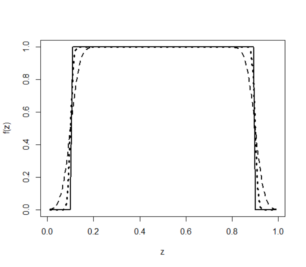
Refer to caption
Figure S1: Illustration of weight functions: the solid black line is the indicator weight function, the dash red line is the smoothed weight function with ϵ=0.001\epsilon=0.001, and the dot blue line is the smoothed weight function with ϵ=0.0001\epsilon=0.0001. As ϵ→0\epsilon\rightarrow 0, the smoothed weight function converges to the indicator function.
Refer to caption
Refer to caption
Refer to caption
Refer to caption
Figure S2: Propensity score distribution by treatment under Propensity Score Design 1–4: Design 1, weak separation and linear predictor; Design 2, strong separation and linear predictor; Design 3, weak separation and non-linear predictor; Design 4, strong separation and non-linear predictor.
Figure S3: Propensity score distribution by AA: the vertical solid lines mark the cut-off values 0.050.05 and 0.60.6 for estimating the average treatment effect, and the vertical dashed line marks the cut-off value 0.70.7 for estimating the average treatment effect on the treated.
Figure S4: Propensity score distribution by AA: the vertical dashed line marks the cut-off value 0.750.75 for estimating the average treatment effect on the treated.