Numerical investigations of non-uniqueness
for the Navier–Stokes initial value problem
in borderline spaces
Abstract
We consider the Cauchy problem for the incompressible Navier–Stokes equations in for a one-parameter family of explicit scale-invariant axi-symmetric initial data, which is smooth away from the origin and invariant under the reflection with respect to the -plane. Working in the class of axi-symmetric fields, we calculate numerically scale-invariant solutions of the Cauchy problem in terms of their profile functions, which are smooth. The solutions are necessarily unique for small data, but for large data we observe a breaking of the reflection symmetry of the initial data through a pitchfork-type bifurcation. By a variation of previous results by Jia & Šverák (2013a) it is known rigorously that if the behavior seen here numerically can be proved, optimal non-uniqueness examples for the Cauchy problem can be established, and two different solutions can exists for the same initial datum which is divergence-free, smooth away from the origin, compactly supported, and locally -homogeneous near the origin. In particular, assuming our (finite-dimensional) numerics represents faithfully the behavior of the full (infinite-dimensional) system, the problem of uniqueness of the Leray–Hopf solutions (with non-smooth initial data) has a negative answer and, in addition, the perturbative arguments such those by Kato (1984) and Koch & Tataru (2001), or the weak-strong uniqueness results by Leray, Prodi, Serrin, Ladyzhenskaya and others, already give essentially optimal results. There are no singularities involved in the numerics, as we work only with smooth profile functions. It is conceivable that our calculations could be upgraded to a computer-assisted proof, although this would involve a substantial amount of additional work and calculations, including a much more detailed analysis of the asymptotic expansions of the solutions at large distances.
Keywords Navier–Stokes equations, Cauchy problem, Leray–Hopf solutions, non-uniqueness, scale-invariant solutions
MSC classes 35A02, 35D30, 35Q30, 76D05, 76D03, 76M10
1 Introduction
We consider the Cauchy problem for the Navier–Stokes equations in ,
| (1) |
Important open questions about the Cauchy problem () concern existence and uniqueness of the solutions in suitable classes of functions. There are essentially two methods to address these issues: the global method based on a priori energy estimates and the local perturbation theory method.
The global method started by the seminal work of Leray (1934) and further developed by Hopf (1950), has lead to the concept of the Leray–Hopf solutions. For , a Leray–Hopf solution of the Cauchy problem in is a field satisfying () weakly, together with some additional requirements, such as the energy inequality
for all , and suitable continuity of the map . We will be dealing with solutions which are smooth for , and have only a weak singularity at , so the exact technical assumptions are not our focus here, although in connection with the scale-invariant solutions one should point out the important generalization by Lemarié-Rieusset (2002); Lemarié-Rieusset (2016), where the global energy requirements are replaced by local ones.
By using the energy estimate and compactness arguments, Leray and others showed the existence of a global Leray–Hopf solution for any with . However, the proof, which relies on compactness arguments, does not give anything concerning uniqueness, except in the case when existence of a more regular solution is known. In that case one can use the energy arguments around the more regular solution, and show that any Leray–Hopf solution has to coincide with the regular one. These results, now known as weak-strong uniqueness theorems, go back to Leray (1934), with later generalizations by a number of authors, including for example Prodi (1959) and Serrin (1963). One has to mention also the results by Kiselev & Ladyzhenskaya (1957), where a slightly different approach is taken.
The perturbation method goes back to Oseen (1911) and Leray (1934) and was later developed in scale-invariant spaces by Fujita & Kato (1962); Fujita & Kato (1964) and Kato (1984). It treats the nonlinearity as a perturbation and inverts the linear part to obtain an integral equation, which is then approached via the Picard iteration. The borderline spaces for this method are scale-invariant with respect to the scaling symmetry of ():
| (2) | ||||
where .
A space for the initial datum is scale-invariant if its norm is invariant under the scaling of the initial condition.
Well-known scale-invariant spaces relevant for the Cauchy problem
() are, for example, the spaces , see Kato (1984),
and , see Koch & Tataru (2001). An important distinction
between the two is that the former does not contain the function ,
whereas the latter does. This is related to the fact that for one can show
local-in-time well-posedness for data of any size (with the time of existence
depending on the datum), whereas for one can only treat small data.
The results in this paper suggest that this is not an artifact of the methods,
but reflects the actual behavior of the solutions.
A special class of initial data being naturally in and not in is given by scale-invariant initial data. An initial datum is scale-invariant under the scaling symmetry () if for all . In particular such initial data behaves like both near the origin and at infinity, so are not in . For scale-invariant initial data, it is natural to look for the solutions of () as being also invariant under the scaling () i.e. satisfying and for all . A scale-invariant solution has the form
where the profiles and satisfy
| (3a) | ||||||
| in together with the condition | ||||||
| (3b) | ||||||
Jia & Šverák (2013a) proved the following global existence result for scale-invariant initial data. A different proof was obtained by Bradshaw & Tsai (2017).
Theorem 1.
If is scale-invariant and divergence-free, then there exists a least one scale-invariant solution of (). Moreover if is a scale-invariant solution then the profile satisfies () and
| (4) |
for any .
The scale-invariant solution is unique for small initial data.
For large initial data it has been conjectured by Jia & Šverák (2013a); Jia & Šverák (2015)
that the scale-invariant solution is not unique.
Our goal is to present numerical evidence for this conjecture.
From the existence of such solutions, the non-uniqueness
of Leray–Hopf solutions and the sharpness of the Serrin uniqueness
criterion can be established along the lines of Jia & Šverák (2015).
In the case of the harmonic map
heat flow, related results have been obtained by Germain et al. (2016).
We now introduce the function spaces needed for the study of (). Let
| (5a) | |||
| where | |||
| (5b) | |||
The profile of a scale-invariant solution belongs naturally to . Let
| (6a) | |||
| with the norm | |||
| (6b) | |||
In view of (), the difference between two different scale-invariant solutions sharing the same initial datum will be in . We define as the following subspace of ,
| (7a) | |||
| with the norm | |||
| (7b) | |||
The subspace of axi-symmetric vector fields in is denoted by . Given some fixed scale-invariant vector-field , we define the map by
| (8) |
where and is chosen such that is divergence-free. Therefore is a solution of () with for if and only if where . The linearization of () around is defined as the operator where
| (9) |
and in particular . The operator is viewed as an unbounded operator in with domain .
For small values of the solution of is unique, leading to a unique solution of (). As long as the kernel of the linearization is trivial, the solution can be (locally) uniquely continued to larger values of . However, if at some value of this kernel is no more trivial then another solution can bifurcate from leading to the non-uniqueness of solutions of ().
The following result on the spectrum of the linearization follows essentially by the results of Gallay & Wayne (2002) and Jia & Šverák (2015).
Theorem 2.
We have:
- 1.
The spectrum of is given by
The eigenvectors corresponding to the continuous part decay at infinity like , whereas the eigenvectors corresponding to decay exponentially fast like . The multiplicity of the eigenvalue is with domain and with the axi-symmetric domain .
- 2.
If , the spectrum of satisfies
(10) where is a discrete set such that is finite for any .
This theorem ensures that only discrete spectrum can cross the imaginary axis. One can establish the following continuation and bifurcation results depending on the behavior of the discrete spectrum:
Theorem 3.
Let and be a solution of , so is a solution of () with .
- 1.
If zero is not in the spectrum , then there exist and a unique smooth solution curve such that and . In particular is a solution of () with .
- 2.
Assume the existence of a smooth solution curve such that . If the spectrum of the linearization has the form
(11) for some , where zero is a simple eigenvalue with associated eigenvector and if
(12) where , then in addition to the solution curve through there exists another unique smooth solution curve through such that , , and .
If the bifurcation is transcritical. If and an additional non-degeneracy assumption is satisfied, we are dealing with a pitchfork bifurcation.
Our aim is to choose a particular scale-invariant vector-field
and to construct numerical solutions exhibiting the bifurcation.
In the situation that we will consider here we will have an additional structure
coming from a -symmetry. The branch will correspond to the solutions
invariant under the -symmetry, whereas the branch will correspond
to the solutions with broken symmetry. The branch itself (as a set) will be invariant
under the symmetry, and hence the bifurcation will necessarily be of pitchfork type,
even though the usual non-degeneracy condition used for pitchfork bifurcations
may not be satisfied.
A possible mechanism behind the ill-posedness can be explained at a heuristic level as follows. Assume the space is filled with an incompressible fluid and consider a portion of the fluid of the shape of a thin disc . If we impose on this portion of the fluid a fast rotation about the -axis with a smooth, albeit sharp transition to zero outside of the disc, the centrifugal force will result in an outward motion of the fluid along the -plane, which will be superimposed on the rotation. One can perhaps compare this outward flux with a jet of fluid, except that our “jet” goes out from the origin in all directions lying in the -plane, rather than just in one direction. Due to incompressibility there must also be an inward flux to the origin, which will take place along the -axis. Assume the velocity field is invariant under the reflection about the -plane. When the field is large, the flow can be expected to be unstable, and any slight deviation from the reflection symmetry will quickly lead to a full breaking of this symmetry. To break the symmetry for smooth solutions, we need an outside impulse. It may be very small, but it cannot be zero. However, the situation may be different for non-smooth initial data. We can imagine a scale-invariant initial datum which resembles a rotation localized in the -plane as much as possible. This can be achieved only to a degree, since the scale-invariance poses its own restrictions, which are of course not compatible with fast decay (among other things). We can still think of as imposing significant rotation in some bounded region of the -plane, but falling off to zero as we move away from the plane. Also, is smooth except at the origin, where it of course cannot be smooth due to the scale invariance (as long as it is non-trivial). Now the symmetry breaking impulse can essentially come from within the singular point, and as such it can be completely hidden from the information provided by the initial datum. In other words, at this level of singularity in the data, the model is asked to operate based on the information which is insufficient for it, somewhat similarly as in the non-uniqueness induced by reverse bubbling in the 2d harmonic map heat flow, see Topping (2002), for example. This analogy is not perfect, as the 2d harmonic map heat flow is critical. For the 3d case we refer the reader to Germain et al. (2016) already quoted above.
The very general method used in perturbation theory or weak-strong uniqueness
breaks down exactly at this point. The numerics presented below suggests that,
at least when well-posedness for rough initial data is concerned, the non-linear
term in the equation does not seem to have any magical properties which would
enable one to go beyond the general perturbation analysis. We emphasize that
this conclusion may not apply to the problem of singularity formation from
smooth data. The situation there may or may not be the similar (see for example
Tao (2016)), but our results say nothing about it. However, if a
singularity is formed, our results suggest that, quite likely, uniqueness may be
lost. The connection between loss of regularity and uniqueness is, of course,
not new. Already in the 1950s, Ladyzhenskaya emphasized the possibility of
non-uniqueness for solutions with insufficient regularity (including the
Leray–Hopf solutions), and Ladyzhenskaya (1967)
presented an example closely related to the scenario discussed in this paper.
Due to our limited computational resources, we will work with axi-symmetric solutions, i.e. solutions which are invariant under the rotations around the -axis. In addition, we consider the -symmetry defined by the reflection with respect to the plane . For the reasons previously explained, we choose the following scale-invariant axi-symmetric divergence-free vector field for the initial data
where denote the cylindrical coordinates. We note that this initial datum has “pure swirl” and is clearly invariant under . In this paper we do not consider the breaking of the axial symmetry, although it is conceivable that for some classes of the initial data this may occur.
The solutions we are dealing with in our work here are defined on the whole space , and hence some truncation of the domain is needed for the numerics. The solutions have good asymptotic expansions for , which in principle could be calculated to a higher order precision. However, the most obvious approximations seem to work quite well for the numerics, and therefore we did not use the higher order expansions. No doubt a possible computer-assisted proof would need to work with more sophisticated approximations for large .
The numerical methods are described in \secrefmethods and our numerical results are presented in \secrefresults, which can be summarized as follows:
Numerical Observations.
We numerically observe the following:
- 1.
In the range , there exists a smooth curve of axi-symmetric and -symmetric self-similar solution of (), with at infinity.
- 2.
The spectrum of the linearization with domain has the form
(13) for some , and there exists such that for , for , and for . Near , the eigenvalue is simple, continuous in and the associated eigenvector is not -symmetric.
- 3.
At there is a supercritical pitchfork-type bifurcation corresponding to the breaking of the symmetry . More precisely, for , in addition to , there exists two axi-symmetric solutions and of () where for and is not -symmetric (hence non trivial) for .
In particular, this suggests that the solutions of the Navier–Stokes equations
are not unique on any time-interval for large initial data in the Lorentz space
. This would mean, that the smallness assumption required by
Lemarié-Rieusset (2016, Theorem 8.2) for proving the local well-posedness
for initial data in is not technical, but reflect the actual nature
of the equations. The same conclusion holds for the result by
Koch & Tataru (2001) for initial data in .
The scale-invariant solutions have infinite energy, however, by following the ideas of Jia & Šverák (2015, Theorem 1.2), the different self-similar solutions can be localized:
Theorem 4.
Assume that () exhibits the same solution behavior as observed in the above reported numerical results. Then there exists and two different axi-symmetric Leray–Hopf solutions of () on with the same compactly supported axi-symmetric initial datum with near the origin. Moreover, these two Leray–Hopf solutions are smooth for and belong to for any with
| (14) |
We note that a Leray–Hopf solution on belongs to for all
| (15) |
by the standard Sobolev embedding. If a Leray–Hopf solution belongs to the Serrin class with
| (16) |
then the solution is unique and smooth (Prodi, 1959; Serrin, 1963; Ladyzhenskaya, 1967; Escauriaza et al., 2003). \Thmreflocalization shows that the Serrin uniqueness criterion is essentially optimal, since non-uniqueness holds for and satisfying (). The Leray–Hopf and Serrin classes are represented on \figrefregion.
Our main focus in this paper is on the numerics, which are presented in \secrefmethods,results. The proofs of \thmrefspectrum-L,continuation-bifurcation,localization are sketched in \secrefspectrum-LU,bifurcation,localization respectively and, in general, go along the lines similar to those in Jia & Šverák (2015).
Notations. The spaces , , and are defined by (), (), and () respectively, and the subspaces of axi-symmetric vector fields are denoted by , , and respectively. The operators and are respectively defined by () and (). The cylindrical coordinates are denoted by . If is a multi-index, we denote by the projection on the elements of , . For example, and .
2 Numerical methods
The restriction to the subspace of axi-symmetric solutions allows to perform the numerical simulations in a two-dimensional domain in the coordinates. We work in the following computational domain
and divide its boundary into two disjoint parts, , where
is the axis boundary and the artificial boundary. As it will become clear later, when the parameter is increasing, the domain as to be also increasing in order to keep the region of interest into the computational domain. Here we choose to work in the domain , where with . This specific factor was chosen such that visually the interesting phenomena are approximately located in the same region of the computational domain for all values of .
The cylindrical coordinates require the following boundary condition on the axis,
The condition () naturally leads to the following boundary condition on ,
The reader not interested in the implementation of the numerical simulations can safely jump to \secrefresults for the description of the numerical results.
2.1 Discretization
The numerical simulations are performed by the finite elements method with the package FEniCS (Logg et al., 2012; Alnæs et al., 2015).
The domain is first discretized into squares each of them split into two triangles, as shown on \figrefmesha. To increase the precision near the origin, this discretization is refined in the square and , which leads to the discretization represented on \figrefmeshb. As already said, we need to work in a domain growing as is increasing. In order to keep the mesh fixed during the continuation in , we instead choose to rescale the equations () in by a factor . That way, the the domain is transformed into the domain and the same mesh can be used for all the values of .
The following weak formulation of () is used
where denotes the scalar product on and and are test functions. The restriction of this weak formulation to axi-symmetric is transformed into cylindrical coordinates and then discretized with Lagrange quadratic polynomials (P2 elements) for and linear polynomials (P1 elements) for .
2.2 Continuation algorithm for
In a first step, a continuation method is used in on the domain . The steps of the continuation method are chosen as for , for and to for . At each step the solution from the previous step is used as an initial datum for a Newton’s method. This Newton’s method typically converges in two or three steps. This method was used because adjusting the step such that only one Newton’s iteration leads to convergence is much too slow. In a second step, the solution founded on is interpolated into the finer mesh . From this initial guess, only one Newton’s iteration leads to a converged solution on in general. All the Newton’s iterations are performed with the MUMPS (Amestoy et al., 2000) linear solver through PETSc (Balay et al., 2016) binding.
2.3 Eigenvalues solver
On , the eigenvalue problem of is given by
with the boundary conditions
and
These equations are solved in the class of axi-symmetric and the discretization used is in the same way as explained in \subrefmethods-discretization. Due to the truncation of the domain, only the eigenvectors of in having a relatively fast decay at infinity will be found. For a local equation in a similar situation it might be reasonable to expect that eigenvectors with exponential decay exist. However, due to non-local effect in the Navier–Stokes equations, the fastest decay one can expect in our problem here is probably , as the terms generated by the original non-linearity need to be projected on divergence-free fields, which creates long-range terms. Therefore, imposing a Dirichlet boundary conditions on the eigenvectors deforms the problem slightly. In practical calculations this effect did not seem to be significant. For a computer-assisted proof this issue would of course have to be carefully addressed. One possibility for this would be to work with the asymptotic expansions at the spatial infinity, as we already discussed above.
In a first step the 36 eigenvalues closest to the real axis were computed for each values of by using the Krylov–Schur algorithm (Hernandez et al., 2009) implemented in SLEPc (Hernandez et al., 2005). Instead of choosing a random initial vector, a linear combination of the eigenvectors founded at the previous step is used, even if the gain in the execution time is not very large.
In a second step, we track the eigenvalues closest to the real axis by a continuation method back to in order to assert that they are not spurious and actually linked to the eigenvalues at . For this continuation by used the Newton’s method (Rall, 1961; Anselone & Rall, 1968) by viewing the eigenvalue problem as a non-linear one with a constraint on the size of the eigenvector.
2.4 Bifurcation from the -symmetric solution
In the scenario where a real eigenvalue is crossing the real axis at , as supposed in the hypotheses of \thmrefcontinuation-bifurcation, then another solution of () should bifurcate from at . This new branch of solution can be also found numerically. For a value of slightly bigger than , Newton’s iterations are performed with the initial guess , where is the eigenvector corresponding to the crossing eigenvalue and is some real parameter to be adjusted such that the Newton’s method converges. When is well chosen, the Newton’s method converges to a solution different from . Finally the continuation algorithm described in \subrefmethods-continuation is used to determine the new branch of solution for larger values of .
3 Numerical results
3.1 Base solution
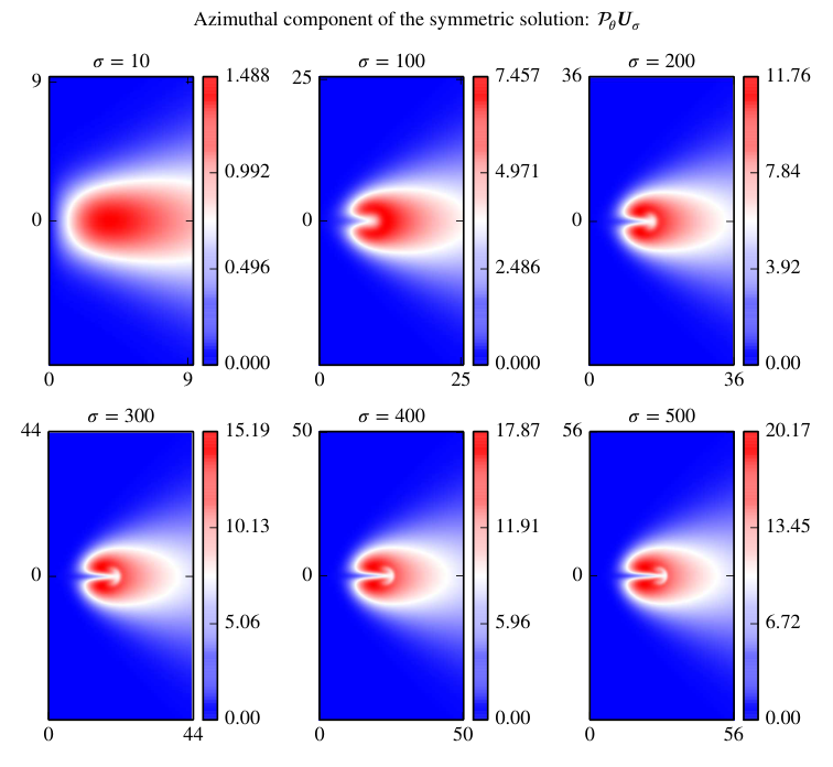
Using the continuation algorithm described in \subrefmethods-continuation, an axi-symmetric and -symmetric solution was found for . This solution is represented on the whole computational domain in \figrefrut,rurz. Near the vertical axis, the radial and azimuthal components of behaves like for small values of has required by the smoothness of the solution. The solutions are -homogeneous on a quite large region near the artificial boundary as shown on \figrefdecay_u,decay_gradu. This means that the choice of the size of the computational domain was large enough. Near the origin, the solution is shown on \figrefurz_small,ut_small,rut_small. As shown on \figrefurz_small, the streamlines projected on the plane are closed, therefore the streamlines of the profile are given by tori as shown on \figrefstream. The first numerical observation 1 concerning the existence of is shown.




3.2 Eigenvalues of
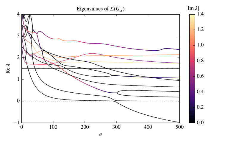
At , the eigenvalues found numerically are given up to a very high precision by for , with multiplicity and correspond exactly to the discrete part found in \thmrefspectrum-L decaying like . The continuous part is not seen numerically due to the polynomial decay of the eigenvectors. The eigenvectors found for are also extremely well-localized, even if numerically the rate cannot be precisely determined due to precision issues. The real part of the eigenvalues closer to the real axis are represented on \figrefspectrum,spectrum_small. In particular a real eigenvalue crosses the real axis near whereas all the other eigenvalues have a strictly positive real part on the range . By going back in , the crossing eigenvalue merges with another real eigenvalues near to form a pair of complex conjugate eigenvalues having a real part close to two. The eigenvalues near the crossing are represented on \figrefspectrum_crossing whereas the eigenvector corresponding to is shown on \figrefeigen_a292 and is not -symmetric. Hence, the second numerical observation claimed 2 is shown.
Interestingly, the eigenvalue is unchanged with respect to . The explanation of this fact comes from the following simple observation, for which we are indebted to a valuable discussion with Hao Jia. The equation () for the profile leads to the following equation for its momentum ,
where is the vorticity of . Therefore, the eigenvalue problem can be transformed into the following equation for the momentum ,
where is the vorticity of . By integrating this last equation over , we obtain the following relation after some integrations by parts,
which explains why the eigenvalue is unchanged even for large values of .


3.3 Bifurcating solution
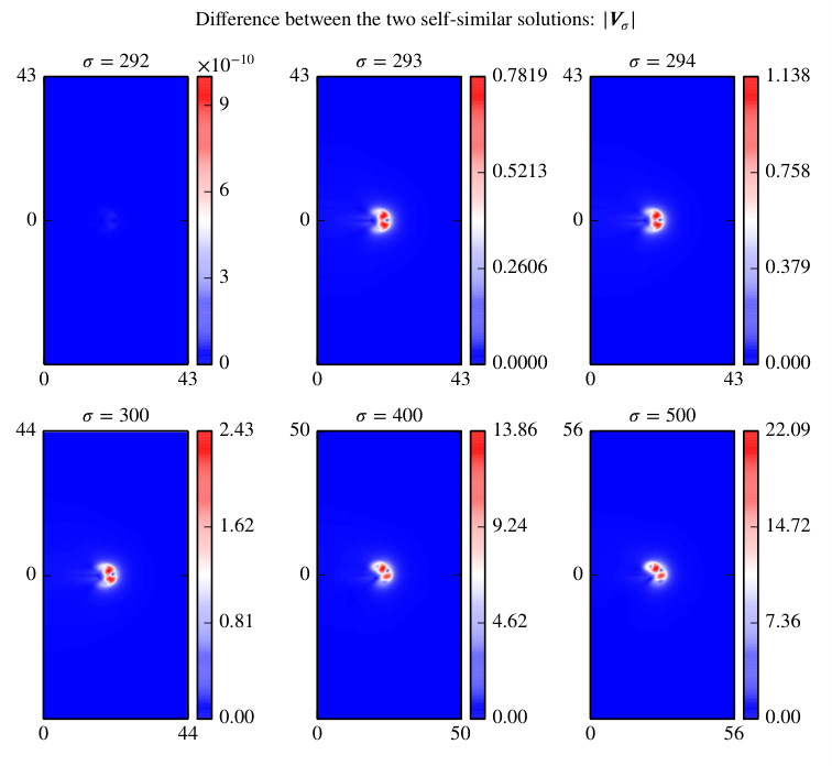
Since a real eigenvalue crossed the real axis near , the method described in \subrefmethods-bifurcation furnish another solution of () bifurcating from . The bifurcating solution is no more visually symmetric with respect to the plane for as shown on \figrefbif_urz,bif_ut,bif_rut. More precisely, for as expected and is growing as increases for as shown on \figrefbif_diff. The reflected solution by the plane is also a solution, so is a supercritical pitchfork-type bifurcation corresponding to the breaking of the -symmetry with respect to the plane . This behavior shows the third numerical observation made 3. By comparing the streamlines of the base solution (\figrefstreama) and of the bifurcating branches and (\figrefstream_bif) at , we see that the topological nature of the streamlines are drastically changed even just after the bifurcation. The reason is that a slight change in the azimuthal component has a large influence on the quasi-periodicity of the streamlines on the tori.



4 Spectrum of
First we determine the point spectrum of :
Proposition 1.
The point spectrum of with domain is given by a continuous part and a discrete part . The eigenvectors of the continuous part decay like at infinity, whereas the discrete part is characterized by eigenvectors decaying exponentially fast like . The multiplicity of is in and in .
Proof.
The point spectrum of is characterized by
| (17) |
so by taking the divergence of the equation, we get , and we can choose . Since is divergence-free, we use the poloidal-toroidal decomposition,
where and are two scalar fields and
Since
and
we obtain that () is transformed into
Both equations being similar, we focus on the second one. Due to the spherical symmetric, the separation of variables can be used in spherical coordinates and the eigenvectors are given by
where are the spherical harmonics and satisfies the following radial equation
| (18) |
In the above, and . Explicitly, we have
and one can check that the unique solution of () leading to continuous and nontrivial fields requires and is given by
where is the Kummer’s confluent hypergeometric function. At large values of , we have
Therefore, the spectrum of () in has a continuous part and a discrete part given by for , characterized by eigenvectors decaying exponentially fast at infinity. The eigenspace corresponding to for is span by with and by with , where in both . For , the eigenspace corresponding to is span by with and by with , always with . Hence the multiplicity of is . In the eigenvectors are characterized by , so the multiplicity of is . ∎
Using \proprefpoint-spectrum, the proof of \thmrefspectrum-L follows by applying results by Gallay & Wayne (2002) and Jia & Šverák (2015):
Proof of \thmrefspectrum-L.
The spectrum of the operator on domain without divergence-free condition, was determined explicitly by Gallay & Wayne (2002, Theorem A.1),
Therefore we directly obtain that . The fact that the spectrum of coincide with the spectrum of follows from \proprefpoint-spectrum.
Since the operator is a relatively compact perturbation of , the essential spectrum is unchanged, and () follows, see Jia & Šverák (2015, Lemma 2.7). ∎
5 Continuation and bifurcation
In this section, we sketch the proof of \thmrefcontinuation-bifurcation, since it follows by applying standard results from the theory of bifurcations:
Proof of \thmrefcontinuation-bifurcation.
First of all, since with continuous embeddings, we directly deduce the continuity of the map defined by (). Therefore, is smooth since it is quadratic.
For the first part, since , then is invertible, so the result follows by applying the implicit function theorem (Kielhöfer, 2012, §I.1).
For the second part, we define , so that . The aim is to find a nontrivial solution of . Since is smooth, we deduce the smoothness of . We have , so
Since is a relatively compact perturbation of , is a Fredholm operator of index zero, hence is a Fredholm operator of index zero. Moreover,
where so by hypothesis . Therefore, we can apply the Crandall–Rabinowitz theorem stated in Kielhöfer (2012, Theorem I.5.1) to obtain a nontrivial smooth curve through such that , and . Then by defining , we obtain that is a smooth solution curve through such that , and . Since , we have
and the nature of the bifurcation follows from the discussion in Kielhöfer (2012, §I.6). We note that the usual non-degeneracy condition for the pitchfork bifurcation may not be satisfied as is quadratic. On the other hand, the reflection symmetry forces the bifurcation to be of the pitchfork type. ∎
6 Localization of self-similar solutions
In this section, we follow the ideas of Jia & Šverák (2015) to obtain solutions with finite energy by truncation of scale-invariant solutions. The space is defined as
| (19) |
equipped with the norm
The space is the subspace of axi-symmetric vector fields in .
By restricting all the spaces to axi-symmetric vector fields, the result of Jia & Šverák (2015, Theorem 1.2) becomes:
Theorem 5.
Let be such that the spectrum of with domain is included in some . Let be such that is sufficiently small depending on and . Let
Let be a divergence-free vector field. Then there exists a time and a unique solution to the generalized Navier–Stokes system with singular lower order terms,
| (20) |
Here the initial condition is satisfied in the sense that
Be using this theorem, we follow the arguments of Jia & Šverák (2015, §5) to localize the two self-similar solutions to :
Proof of \thmreflocalization.
By assuming that our numerical results reflect the actual behavior of the solutions, we obtain the existence of two different axi-symmetric self-similar solutions and for satisfying () with the same initial datum ,
By choosing close enough to , we can assume that the crossing eigenvalue in () satisfies and moreover, we can make small enough to apply \thmrefns-singular. By a cutoff of the stream function associated to , we can write , where is a divergence-free vector field of compact support in and equal to on and is a divergence-free vector field such that . By taking large enough, we can apply \thmrefns-singular with initial data , , and , to obtain a solution of (). Therefore is an axi-symmetric solution of the Navier–Stokes system () with initial data . In the same way, by applying \thmrefns-singular with initial data , , and , we obtain a solution of (), so that is an axi-symmetric solution of the Navier–Stokes system () with initial data . By the standard regularity theory of the Navier–Stokes equations , so by using \thmrefjia-sverak, we obtain that . Since , one can show that and are Leray–Hopf solutions, for example by using the results of Jia & Šverák (2013b, Lemma 2.2).
We now prove that and are not equal. Since and are uniformly bounded in , we see that
is unbounded as , and therefore and are not equal since is not trivial.
We now prove that and belong to the complement of Serrin class. Since , we obtain that , so for . By interpolation, we obtain for
| (21) |
as drawn on \figrefregion. We split the space into where is the ball of radius one centered at the origin and its complement. By using the explicit decay () of the self-similar solutions, we obtain that for and therefore also for . In the same way, we can prove that for , so for and satisfying (). Since , by interpolation we obtain that for and . Therefore we proved that for and . The same procedure applies to and the proof is finished. ∎
Acknowledgments
The authors would like to thank J. Gómez-Serrano, H. Jia, and V. Vicol for valuable discussions and comments. Parts of this work were done while J. Guillod was at the School of Mathematics of the University of Minnesota, the Mathematics Department of Princeton University, and the ICERM at Brown University. The hospitality and facilities of these institutions are gratefully acknowledged. The research of J. Guillod was supported by the Swiss National Science Foundation grants 161996 and 171500. The research of V. Šverák was partially supported by grant DMS 1362467 from the National Science Foundation.
References
- Alnæs et al. (2015) Alnæs, M. S., Blechta, J., Hake, J., Johansson, A., Kehlet, B., Logg, A., Richardson, C., Ring, J., Rognes, M. E., & Wells, G. N. 2015, The FEniCS project version 1.5. Archive of Numerical Software 3 (100), 9–23, 10.11588/ans.2015.100.20553
- Amestoy et al. (2000) Amestoy, P., Duff, I., & L’Excellent, J.-Y. 2000, Multifrontal parallel distributed symmetric and unsymmetric solvers. Computer Methods in Applied Mechanics and Engineering 184 (2-4), 501–520, 10.1016/s0045-7825(99)00242-x
- Anselone & Rall (1968) Anselone, P. M. & Rall, L. B. 1968, The solution of characteristic value-vector problems by Newton’s method. Numerische Mathematik 11 (1), 38–45, 10.1007/bf02165469
- Balay et al. (2016) Balay, S., Abhyankar, S., Adams, M. F., Brown, J., Brune, P., Buschelman, K., Dalcin, L., Eijkhout, V., Gropp, W. D., Kaushik, D., Knepley, M. G., McInnes, L. C., Rupp, K., Smith, B. F., Zampini, S., Zhang, H., & Zhang, H. 2016, PETSc users manual. Tech. Rep. ANL-95/11 - Revision 3.7, Argonne National Laboratory
- Bradshaw & Tsai (2017) Bradshaw, Z. & Tsai, T.-P. 2017, Forward discretely self-similar solutions of the Navier–Stokes equations II. Annales Henri Poincaré 18 (3), 1095–1119, 10.1007/s00023-016-0519-0
- Escauriaza et al. (2003) Escauriaza, L., Seregin, G., & Šverák, V. 2003, -solutions of the Navier–Stokes equations and backward uniqueness. Russian Mathematical Surveys 58 (2), 211–250, 10.1070/rm2003v058n02abeh000609
- Fujita & Kato (1962) Fujita, H. & Kato, T. 1962, On the nonstationary Navier–Stokes system. Rendiconti del Seminario Matematico della Università di Padova 32, 243–260
- Fujita & Kato (1964) Fujita, H. & Kato, T. 1964, On the Navier–Stokes initial value problem. I. Archive for Rational Mechanics and Analysis 16 (4), 269–315, 10.1007/bf00276188
- Gallay & Wayne (2002) Gallay, T. & Wayne, C. E. 2002, Invariant manifolds and the long-time asymptotics of the Navier–Stokes and vorticity equations on . Archive for Rational Mechanics and Analysis 163 (3), 209–258, 10.1007/s002050200200
- Germain et al. (2016) Germain, P., Ghoul, T.-E., & Miura, H. 2016, On uniqueness for the harmonic map heat flow in supercritical dimensions, arXiv:1601.06601
- Hernandez et al. (2009) Hernandez, V., Roman, J. E., Tomas, A., & Vidal, V. 2009, Krylov–Schur methods in SLEPc. Tech. Rep. STR-7, Universitat Politècnica de València, available at http://slepc.upv.es
- Hernandez et al. (2005) Hernandez, V., Roman, J. E., & Vidal, V. 2005, SLEPc. ACM Transactions on Mathematical Software 31 (3), 351–362, 10.1145/1089014.1089019
- Hopf (1950) Hopf, E. 1950, Über die Anfangswertaufgabe für die hydrodynamischen Grundgleichungen. Mathematische Nachrichten 4 (1–6), 213–231, 10.1002/mana.3210040121
- Jia & Šverák (2013a) Jia, H. & Šverák, V. 2013a, Local-in-space estimates near initial time for weak solutions of the Navier–Stokes equations and forward self-similar solutions. Inventiones mathematicae 196 (1), 233–265, 10.1007/s00222-013-0468-x
- Jia & Šverák (2013b) Jia, H. & Šverák, V. 2013b, Minimal -initial data for potential Navier–Stokes singularities. SIAM J. Math. Anal. 45 (3), 1448–1459, 10.1137/120880197
- Jia & Šverák (2015) Jia, H. & Šverák, V. 2015, Are the incompressible 3d Navier–Stokes equations locally ill-posed in the natural energy space? Journal of Functional Analysis 268 (12), 3734–3766, 10.1016/j.jfa.2015.04.006
- Kato (1984) Kato, T. 1984, Strong -solutions of the Navier–Stokes equation in , with applications to weak solutions. Mathematische Zeitschrift 187 (4), 471–480, 10.1007/BF01174182
- Kielhöfer (2012) Kielhöfer, H. 2012, Bifurcation Theory: An Introduction with Applications to Partial Differential Equations, vol. 156. Springer New York, 10.1007/978-1-4614-0502-3
- Kiselev & Ladyzhenskaya (1957) Kiselev, A. A. & Ladyzhenskaya, O. A. 1957, On the existence and uniqueness of the solution of the nonstationary problem for a viscous, incompressible fluid. Izv. Akad. Nauk SSSR. Ser. Mat. 21, 655–680
- Koch & Tataru (2001) Koch, H. & Tataru, D. 2001, Well-posedness for the Navier-Stokes equations. Advances in Mathematics 157 (1), 22–35, 10.1006/aima.2000.1937
- Ladyzhenskaya (1967) Ladyzhenskaya, O. A. 1967, On uniqueness and smoothness of generalized solutions to the Navier–Stokes equations. Zapiski Nauchnykh Seminarov POMI 5, 169–185
- Lemarié-Rieusset (2002) Lemarié-Rieusset, P. G. 2002, Recent developments in the Navier–Stokes problem. CRC Research Notes in Mathematics Series, CRC Press, 10.1201/9781420035674
- Lemarié-Rieusset (2016) Lemarié-Rieusset, P. G. 2016, The Navier–Stokes Problem in the 21st Century. CRC Press, 10.1201/b19556
- Leray (1934) Leray, J. 1934, Sur le mouvement d’un liquide visqueux emplissant l’espace. Acta Mathematica 63, 193–248, 10.1007/BF02547354
- Logg et al. (2012) Logg, A., Mardal, K.-A., Wells, G. N., et al. 2012, Automated Solution of Differential Equations by the Finite Element Method. Springer, 10.1007/978-3-642-23099-8
- Oseen (1911) Oseen, C. W. 1911, Sur les formules de Green généralisées qui se présentent dans l’hydrodynamique et sur quelques-unes de leurs applications. Acta Mathematica 34 (1), 205–284, 10.1007/BF02393128
- Prodi (1959) Prodi, G. 1959, Un teorema di unicità per le equazioni di Navier–Stokes. Annali di Matematica 48 (1), 173–182, 10.1007/bf02410664
- Rall (1961) Rall, L. B. 1961, Newton’s method for the characteristic value problem . Journal of the Society for Industrial and Applied Mathematics 9 (2), 288–293
- Serrin (1963) Serrin, J. 1963, The initial value problem for the Navier–Stokes equations. In Nonlinear problems (edited by R. E. Langer), 69–98, The University of Wisconsin Press
- Tao (2016) Tao, T. 2016, Finite time blowup for an averaged three-dimensional Navier–Stokes equation. Journal of the American Mathematical Society 29 (3), 601–674, 10.1090/jams/838
- Topping (2002) Topping, P. 2002, Reverse bubbling and nonuniqueness in the harmonic map flow. International Mathematics Research Notices (10), 505–520, 10.1155/S1073792802105083