A Class of Temporal Hierarchical Exponential Random Graph Models for Longitudinal Network Data
Abstract
As a representation of relational data over time series, longitudinal networks provide opportunities to study link formation processes. However, networks at scale often exhibits community structure (i.e. clustering), which may confound local structural effects if it is not considered appropriately in statistical analysis. To infer the (possibly) evolving clusters and other network structures (e.g. degree distribution and/or transitivity) within each community, simultaneously, we propose a class of statistical models named Temporal Hierarchical Exponential Random Graph Models (THERGM). Our generative model imposes a Markovian transition matrix for nodes to change their membership, and assumes they join new community in a preferential attachment way. For those remaining in the same cluster, they follow a specific temporal ERG model (TERGM). While a direct MCMC based Bayesian estimation is computational infeasible, we propose a two-stage strategy. At the first stage, a specific dynamic latent space model will be used as the working model for clustering. At the second stage, estimated memberships are taken as given to fit a TERG model in each cluster. We evaluate our methods on simulated data in terms of the mis-clustering rate, as well as the goodness of fit and link prediction accuracy.
keywords
Longitudinal network data; Temporal Hierarchical Exponential Random Graph Models; Dynamic Latent Space Models; Clustering;1 Introduction
Relational data over a series of time points are becoming more available as the information technology advances, for example, [32] study flu transmission by using sensors to record human contact in a high school. One of the most attractive topics in network research is community detection or clustering (see [5] for a review). Speaking of scientific literatures, communities could be corresponding to research fields. Those fields may or may not be pre-specified, take the “network research community” as example, it has seen mixed contributions and gaining momentums from scholars in Physics, Computer Science, Sociology, Statistics and other disciplines [29, 45, 20]. Multiple snapshots, or even at the finest grain as a stream of relational events, provide more information than a static network. It provides us opportunities to capture the trajectories of evolving network structures, with applications to trend analysis [26] and link prediction [33].
Besides the community structure, there could be various types of network effects going on locally. For example, the common sense that “my friends’ friends are more likely to be my friends” and “people with same interests are more likely to be friends” are typically referred to as transitivity and homophily, respectively. With a long history of being studied by Sociologists [8, 28], such kind of network structures can be flexibly specified and therefore estimated/tested by a powerful statistical tool called Exponential Random Graph Models (ERGM) [6, 46]. We should have reasonable suspect that transitivity or homophily acts equally in different communities and it would be natural to construct a statistical model that consider local structural effects as well as clustering, which represents a more macro level structure. However, current works for large-scale network structure analysis have mostly been limited to base on the Stochastic Block Models (SBM) [17, 39], which assumes no dependence among ties within the same block (cluster). SBM is adopted for its simplicity in the hope that it approximates well from the perspective of an efficient clustering estimator. Nice statistical properties have been established for computationally effective algorithmic methods such as spectral clustering, under both the static [31, 30, 21] and dynamic [9] settings. While efforts are being made to extend this often over-simplified family of models to a boarder class [44], ERGM is generally considered having degeneracy problem [12] and too expensive to compute the MCMC approximated MLE [38]. In fact, significant improvement on model specification and estimation technique has been made [40, 19, 18] for the past decade. More importantly, the longitudinal extensions of ERGM rarely suffer from the model degeneracy problem [13]. It can be intuitively understood as that structural effects became much more clear when the changes are explicitly modeled, rather than being very likely blurred in a cumulative snapshot.
In this paper, we propose a class of Temporal Hierarchical Exponential Random Graph Models (THERGM) to fully utilize the information contained in longitudinal network data, which may greatly improve the overall goodness of fit and link prediction accuracy. It seems that we pay the price of a non-scalable inference procedure in order to gain the modeling power of ERGM, but fortunately, [25] suggests that roughly 100 nodes is probably a universal "natural size" of a meaningful cluster, including social, information, Internet and biological networks. While this is the right scale that current ERGM implementation [10] could be routinely carried out, it is still computationally infeasible to directly combine with the community structure in a straightforward Bayesian approach. To tackle this problem, we propose a two-stage strategy that uses a Dynamic Latent Space Model [16, 35, 36] to do the clustering at the first stage. That working model should be corresponded to the particular ERG Model you choose as specifically as possible. For example, a distance measure or some covariates should be included if the (hypothesized) true model contains transitivity or homophily effect, respectively. A Latent Space Model that accounts for all dependencies among relational ties plus an appropriate model of community evolution could be expected to recover the clustering change trajectory asymptotically. Then at the second stage, we take the clustering estimates at each time point as given, and further fit a temporal ERG model for actors remaining in each community. In this way, we harness the describing power of more complex models (THERGM versus dynamic SBM) in a timely manner by having the sizes after decomposition under control. For researchers who only care about the inference of (temporal) ERGM, our approach could provide correctness, rather than feasibility, as it could be easily confounded by the hierarchical structure if there are unknown clusters.
The rest of paper is organized as following: In Section 2, we briefly state the form of Exponential Random Graph Models. In Section 3 we propose our new Hierarchical ERGM for temporal clustered network data. In Section 4, we describe the two-phase strategy for inference. In Section 5, various simulation settings for our generative models are used to evaluate the performance of the proposed two-phase strategy. We summarize contributions and discuss limitations as well as future work in Section 6.
2 Related Works
2.1 Exponential Random Graph Models
Exponential Random Graph Models is a family of statistical models taking the following form of the probability functions
| (1) |
with arbitrary statistics for researchers to specify structures of scientific interests. The interpretation of parameters is typically based on the log odds ratio of forming a tie, conditional on the rest of the graph since:
| (2) |
where represents all other ties except , is the change statistic with and denoting the adjacency matrices with the th element equal to and while all others are the same as .
2.2 Hierarchical ERGM
[34] proposed a hierarchical extension of ERGM by introducing the local dependence that breaks down the dependence of random graph into subgraphs. Assume there is a partition of the vertices V into non-empty finite subsets , such that the within- and between- neighbourhood subgraphs given membership satisfy
| (3) |
The within-neighborhood probability measures take specific ERGM forms as
| (4) |
whereas the between-neighborhood probability measures induce independence between subgraphs, and the between-neighborhood ties are assumed to be independent
| (5) |
2.3 Temporal ERGM
[13] proposed a temporal extension of ERGM by making a Markov assumption on the network from one time step to the next. Specifically, is independent of given . Taking the first observation as given, the joint distribution can be factorized:
| (6) |
Given the Markov assumption, ERGM is generalized for evolving networks assuming admits an ERGM representation. The conditional PDF takes the following form:
| (7) |
The normalizing constant now also depends on , it is still intractable and the same MCMC approximated MLE techniques apply.
[23] further extended the discrete Temporal ERGM to a separate parameterization of incidence from duration, motived by the reality that social processes and factors of ties forming are very likely not the same as those of ties dissolving.
2.4 Other Temporal Models
Another popular class of models for dynamic networks is Stochastic Actor-Oriented Models (SAOM) [37, 41]. [24] explains how SAOM has an ERGM as its limiting distribution under a specific but rarely applied rate function. TERGM outperforms SAOM substentially when the DSP of SAOM was not met so TERGM is more robust in the sense of model mis-specification. [22] models the birth and death of individual groups via a distance dependent Indian Buffet Process and capture the evolution of node group memberships via a Factorial Hidden Markov model.
3 Temporal Hierarchical ERGM
We begin with notations. Consider a temporal series of networks , where represents the network observed at time , consisting a set of vertices and edges . We assume a fixed number of communities(or clusters, neighborhoods, blocks), and each vertex has a membership(or color) for , which may vary at a different time . The distribution of communities is also allowed to change, as it reflects the overall trend of the system, for example, the rising of “big data” in Statistics. In this paper, is restricted to a binary adjacency matrix where
Most of the literature assume that for all is a fixed set over time, while any dynamically changing network in real world would have nodes entering or leaving the system. It is because of that network structural analysis are concerning about the effects of existing ties on the formation (or dissolution) of future relations, which are implicitly among the same set of nodes. If the nodes change too volatile, it is the reason(s) of entering (leaving) should be modeled. For example, during the first 3 months from the launch of facebook.com, what really matters is how to attract people to open accounts, rather than introducing friends’ friends. Here we further assume this situation applies to the community level. That is to say, for subsets and of vertices belonging to community at any two consecutive time points, the remaining part is at least a significant portion of the union . Together with a finite and pre-fixed number of clusters , we are targeting a gradually evolving system. For streaming graph data, see for example [2].
3.1 Our model
Now we propose a class of Temporal Hierarchical Exponential Random Graph Models (THERGM), by assuming 1. can be decomposed by the current clustering at any time ; 2. Markov property of the temporal dependency on and also implicitly :
Denote as the set of remaining nodes in group during the time and , so that and are the subgraphs spanned by the common nodes at time and , respectively. and are the corresponding adjacency matrices:
| (8) |
Note the first item in the RHS of equation 8 accounts for the ties associated with remaining nodes in group , which takes the temporal ERGM form:
Note that it is implicitly depending on and .
The second item accounts for the ties associated with nodes newly joined group from time to time , which can be assumed to follow a preferential attachment process [3].
The third item accounts for the between-neighborhood ties, which are assumed to be independent as in equation 5.
To complete the THERGM specification, a sensible layer of community evolution is needed. Similar to longitudinal network observations, Markovian assumptions are made to simplify the joint distribution
and there are at least three ways to do it:
- •
- •
- •
[7] propose that with probability , each node keeps its label from one time step to the next, otherwise it chooses a new label from the prior . The transition probability for community memberships is
(9)
We adopt the first way of modeling, and implicitly assume that the community evolution does not depend on the realized networks. See latent feature propagation model of [14], to capture the phenomenon that observed social interactions from the past can also affect future unobserved structure. The proposed dynamic process can be illustrated in Figure 1:

4 Model inference
A straightforward full Bayesian approach to estimate THERGM parameters is not practical. At the clustering level, the sample space of membership is where is the number of blocks and is the number of nodes. At the within-block TERGM part, the sample size of edge variable is where is the number of nodes in th block (each pair of nodes can have a link present or absent in an undirected binary network). So both parts need MCMC or other sampling methods to do the approximation, directly combining them makes the problem intractable. In this section, we propose a two-stage strategy to tackle this problem.
4.1 Clustering with a working model
Now, we temporarily jump out of the ERGM paradigm and take a look at another class of statistical models that mainly embracing the classical latent factor idea. Instead of explicitly modeling dependence, the Latent Structure Models (LSM) postulate latent nodal variables and conditional independence of given those variables and .
[16] introduced the concept of unobserved "social space" within which each node has a position so that a tie is independent of all others given the unobserved positions of the pair it connects to:
| (10) |
where are observed covariates, and and are parameters and positions to be estimated. [11] took a subclass Distance Models where the probability of a tie is modeled as a function of some measure of distance between the latent space positions of two nodes:
| (11) |
with restriction of for the identification purpose. Then they imposed a finite mixture of multivariate Gaussian distribution for to represent clustering:
| (12) |
where non-negative is the probability that an individual belongs to the th group, with .
[36] proposed a dynamic extension of LSM, assuming at each time point, each node belongs to one of a fixed number of clusters, and the membership may change over time. Denote the latent position of node at time as and the corresponding membership as . Let and , with the additional assumption that given the latent positions , and , , are conditionally independent, the decomposition follows:
| (13) |
Two assumptions are made on the latent positions and the cluster assignments. First, the cluster assignments are assumed to follow a Markov process, i.e.,
| (14) |
Second, given the current cluster assignment and all previous cluster assignments and latent positions, we assume the current latent positions depend only on the previous latent position and the current cluster assignments, i.e.,
| (15) |
4.2 Identification and label switching
The cluster label is identified up to a permutation. We adopted the hamming error definition to define a correct membership, which is the minimal clustering errors over a permutation of the set . See section of [21] for details. Here we want to make explicitly an assumption that the label switching problem between two consecutive time steps can be solved by the permutation of the hamming error. This assumption could be easily satisfied when the temporal changes are not very dramatic.
5 Experiments
5.1 Simulation setting
We use Dynamic Stochastic Block Model (DSBM) [27] as a comparison.
The dissolving rate is set to time steps. The initial density is set to be and kept roughly stable if without the transitivity effect. Other parameters are … All the simulations are carried out using the R package Simulator [4].
One example of the simulated longitudinal networks, with some summary statistics are shown in Figure 2:

5.2 Transition matrix estimate
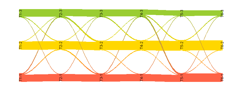
In a lot of applications, the overall trend of the communities change, for example, the rising of a certain group. The following river plot is an illustration of how nodes “flow” from one “river” into another. The height of each bar, in other words, the width of each river, represents the relative size of that community, illustrated in Figure 3.
5.3 Evolving membership estimate
We investigate the effects of sample size (per cluster) and the transitivity strength under four scenarios, which are the combination of two factors: the time transition rate (slow v.s. quick) and within cluster density (easy when the difference of within- and between- cluster density is large). The results in Figure 4 indicate that when it is slow and easy, all methods perform well, while under quicker or harder situations, the dynamic latent space model perform better as it is a better working model.

If we dig into the longitudinal mis-clustering rates, we can see that DSBM has a non-negligible probability that error rate could not be controlled, while DLSM can as shown in Figure 5.

5.4 Cluster specific ERGM estimate
The TERGM estimates conditioned on the membership estimates in the first step is carried out by [23]. Results illustrated in Figure 6.

5.5 Goodness of fit
To answer the natural question that if my working model is already good enough, why bother fitting within-cluster TERGMs, we show Figure 7.


5.6 Link prediction
As in a lot of machine learning applications, the out-of-sample prediction accuracy is the most trustworthy metric. So we conducted a one time step out-of-sample prediction and calculated the Area Under the ROC curves (AUC) in Figure 8.

6 Discussion and future work
As the experiments show, the clustering performance is not perfect, and the mis-clustered nodes have huge impact on the second stage TERGM inference. We are currently working on an augmented Bayesian method to jointly infer the clustering and local structures. The tool we use is the newly developed probabilistic programming language Edward [43, 42], which integrates the Google Tensorflow [1] framework with its capability to utilize GPU.
References
- [1] M. Abadi, A. Agarwal, P. Barham, E. Brevdo, Z. Chen, C. Citro, G. S. Corrado, A. Davis, J. Dean, M. Devin, et al. Tensorflow: Large-scale machine learning on heterogeneous distributed systems. arXiv preprint arXiv:1603.04467, 2016.
- [2] C. C. Aggarwal, Y. Zhao, and S. Y. Philip. On clustering graph streams. In SDM, pages 478–489. SIAM, 2010.
- [3] A.-L. Barabási and R. Albert. Emergence of scaling in random networks. science, 286(5439):509–512, 1999.
- [4] J. Bien. The simulator: An engine to streamline simulations. arXiv preprint arXiv:1607.00021, 2016.
- [5] S. Fortunato. Community detection in graphs. Physics reports, 486(3):75–174, 2010.
- [6] O. Frank and D. Strauss. Markov graphs. Journal of the american Statistical association, 81(395):832–842, 1986.
- [7] A. Ghasemian, P. Zhang, A. Clauset, C. Moore, and L. Peel. Detectability thresholds and optimal algorithms for community structure in dynamic networks. arXiv preprint arXiv:1506.06179, 2015.
- [8] M. S. Granovetter. The strength of weak ties. American journal of sociology, pages 1360–1380, 1973.
- [9] Q. Han, K. S. Xu, and E. M. Airoldi. Consistent estimation of dynamic and multi-layer block models. arXiv preprint arXiv:1410.8597, 2014.
- [10] M. S. Handcock, D. R. Hunter, C. T. Butts, S. M. Goodreau, and M. Morris. statnet: Software tools for the representation, visualization, analysis and simulation of network data. Journal of statistical software, 24(1):1548, 2008.
- [11] M. S. Handcock, A. E. Raftery, and J. M. Tantrum. Model-based clustering for social networks. Journal of the Royal Statistical Society: Series A (Statistics in Society), 170(2):301–354, 2007.
- [12] M. S. Handcock, G. Robins, T. A. Snijders, J. Moody, and J. Besag. Assessing degeneracy in statistical models of social networks. Technical report, Citeseer, 2003.
- [13] S. Hanneke, W. Fu, E. P. Xing, et al. Discrete temporal models of social networks. Electronic Journal of Statistics, 4:585–605, 2010.
- [14] C. Heaukulani and Z. Ghahramani. Dynamic probabilistic models for latent feature propagation in social networks. In Proceedings of the 30th International Conference on Machine Learning (ICML-13), pages 275–283, 2013.
- [15] Q. Ho, L. Song, and E. P. Xing. Evolving cluster mixed-membership blockmodel for time-evolving networks. In International Conference on Artificial Intelligence and Statistics, pages 342–350, 2011.
- [16] P. D. Hoff, A. E. Raftery, and M. S. Handcock. Latent space approaches to social network analysis. Journal of the american Statistical association, 97(460):1090–1098, 2002.
- [17] P. W. Holland, K. B. Laskey, and S. Leinhardt. Stochastic blockmodels: First steps. Social networks, 5(2):109–137, 1983.
- [18] R. M. Hummel, D. R. Hunter, and M. S. Handcock. Improving simulation-based algorithms for fitting ergms. Journal of Computational and Graphical Statistics, 21(4):920–939, 2012.
- [19] D. R. Hunter and M. S. Handcock. Inference in curved exponential family models for networks. Journal of Computational and Graphical Statistics, 15(3), 2006.
- [20] M. O. Jackson et al. Social and economic networks, volume 3. Princeton university press Princeton, 2008.
- [21] J. Jin. Fast community detection by score. The Annals of Statistics, 43(1):57–89, 2015.
- [22] M. Kim and J. Leskovec. Nonparametric multi-group membership model for dynamic networks. In Advances in neural information processing systems, pages 1385–1393, 2013.
- [23] P. N. Krivitsky and M. S. Handcock. A separable model for dynamic networks. Journal of the Royal Statistical Society: Series B (Statistical Methodology), 76(1):29–46, 2014.
- [24] P. Leifeld and S. J. Cranmer. A theoretical and empirical comparison of the temporal exponential random graph model and the stochastic actor-oriented model. arXiv preprint arXiv:1506.06696, 2015.
- [25] J. Leskovec, K. J. Lang, A. Dasgupta, and M. W. Mahoney. Community structure in large networks: Natural cluster sizes and the absence of large well-defined clusters. Internet Mathematics, 6(1):29–123, 2009.
- [26] J. Leskovec, M. McGlohon, C. Faloutsos, N. S. Glance, and M. Hurst. Patterns of cascading behavior in large blog graphs. In SDM, volume 7, pages 551–556. SIAM, 2007.
- [27] C. Matias and V. Miele. Statistical clustering of temporal networks through a dynamic stochastic block model. Journal of the Royal Statistical Society: Series B (Statistical Methodology), 2017.
- [28] M. McPherson, L. Smith-Lovin, and J. M. Cook. Birds of a feather: Homophily in social networks. Annual review of sociology, pages 415–444, 2001.
- [29] M. Newman, A.-L. Barabasi, and D. J. Watts. The structure and dynamics of networks. Princeton University Press, 2011.
- [30] T. Qin and K. Rohe. Regularized spectral clustering under the degree-corrected stochastic blockmodel. In Advances in Neural Information Processing Systems, pages 3120–3128, 2013.
- [31] K. Rohe, S. Chatterjee, and B. Yu. Spectral clustering and the high-dimensional stochastic blockmodel. The Annals of Statistics, pages 1878–1915, 2011.
- [32] M. Salathé, M. Kazandjieva, J. W. Lee, P. Levis, M. W. Feldman, and J. H. Jones. A high-resolution human contact network for infectious disease transmission. Proceedings of the National Academy of Sciences, 107(51):22020–22025, 2010.
- [33] P. Sarkar, D. Chakrabarti, and M. Jordan. Nonparametric link prediction in large scale dynamic networks. Electron. J. Statist., 8(2):2022–2065, 2014.
- [34] M. Schweinberger and M. S. Handcock. Local dependence in random graphs: characterization, properties, and statistical inference. Journal of the Royal Statistical Society: Series B (Statistical Methodology), 2015.
- [35] D. K. Sewell and Y. Chen. Latent space models for dynamic networks. Journal of the American Statistical Association, (just-accepted):00–00, 2014.
- [36] D. K. Sewell, Y. Chen, et al. Latent space approaches to community detection in dynamic networks. Bayesian Analysis, 2016.
- [37] T. A. Snijders. The statistical evaluation of social network dynamics. Sociological methodology, 31(1):361–395, 2001.
- [38] T. A. Snijders. Markov chain monte carlo estimation of exponential random graph models. Journal of Social Structure, 3(2):1–40, 2002.
- [39] T. A. Snijders and K. Nowicki. Estimation and prediction for stochastic blockmodels for graphs with latent block structure. Journal of classification, 14(1):75–100, 1997.
- [40] T. A. Snijders, P. E. Pattison, G. L. Robins, and M. S. Handcock. New specifications for exponential random graph models. Sociological methodology, 36(1):99–153, 2006.
- [41] T. A. Snijders, G. G. Van de Bunt, and C. E. Steglich. Introduction to stochastic actor-based models for network dynamics. Social networks, 32(1):44–60, 2010.
- [42] D. Tran, M. D. Hoffman, R. A. Saurous, E. Brevdo, K. Murphy, and D. M. Blei. Deep probabilistic programming. In International Conference on Learning Representations, 2017.
- [43] D. Tran, A. Kucukelbir, A. B. Dieng, M. Rudolph, D. Liang, and D. M. Blei. Edward: A library for probabilistic modeling, inference, and criticism. arXiv preprint arXiv:1610.09787, 2016.
- [44] Y. Wan and M. Meila. A class of network models recoverable by spectral clustering. In Advances in Neural Information Processing Systems, pages 3267–3275, 2015.
- [45] S. Wasserman and K. Faust. Social network analysis: Methods and applications, volume 8. Cambridge university press, 1994.
- [46] S. Wasserman and P. Pattison. Logit models and logistic regressions for social networks: I. an introduction to markov graphs andp. Psychometrika, 61(3):401–425, 1996.
- [47] E. P. Xing, W. Fu, and L. Song. A state-space mixed membership blockmodel for dynamic network tomography. Ann. Appl. Stat., 4(2):535–566, 06 2010.
- [48] T. Yang, Y. Chi, S. Zhu, Y. Gong, and R. Jin. Detecting communities and their evolutions in dynamic social networksa bayesian approach. Machine learning, 82(2):157–189, 2011.