A quasinonlocal coupling method for nonlocal and local diffusion modelsThanks: The research of Q. Du and X. Tian is supported in part by the U.S. NSF grants DMS-1719699, AFOSR grant FA9550-14-1-0073 MURI Center for Material Failure Prediction through peridynamics and the ARO MURI Grant W911NF-15-1-0562. The work of X. Li is supported in part by the Simons Collaboration Grant with Award ID: 426935 and NSF DMS-1720245. The work of J. Lu is supported in part by the National Science Foundation under award DMS-1454939.

Qiang Du Email address: qd2125@columbia.edu Address: Department of Applied Physics and Applied Mathematics, Columbia University, New York, NY 10027. . , Xingjie Helen Li Email address: xli47@uncc.edu Address: Department of Mathematics and Statistics, University of North Carolina at Charlotte, Charlotte NC 28223. . , Jianfeng Lu Email address: jianfeng@math.duke.edu Address: Department of Mathematics, Department of Physics, Department of Chemistry, Duke University, Box 90320, Durham, NC 27708. . and Xiaochuan Tian Email address: xt2156@columbia.edu Email address: xtian@math.utexas.edu Address: Department of Applied Physics and Applied Mathematics, Columbia University, New York, NY 10027. . Current address: Department of Mathematics, University of Texas at Austin, Austin, TX 78712. .

Abstract.

In this paper, we extend the idea of “geometric reconstruction” to couple a nonlocal diffusion model directly with the classical local diffusion in one dimensional space. This new coupling framework removes interfacial inconsistency, ensures the flux balance, and satisfies energy conservation as well as the maximum principle, whereas none of existing coupling methods for nonlocal-to-local coupling satisfies all of these properties. We establish the well-posedness and provide the stability analysis of the coupling method. We investigate the difference to the local limiting problem in terms of the nonlocal interaction range. Furthermore, we propose a first order finite difference numerical discretization and perform several numerical tests to confirm the theoretical findings. In particular, we show that the resulting numerical result is free of artifacts near the boundary of the domain where a classical local boundary condition is used, together with a coupled fully nonlocal model in the interior of the domain.

Key words and phrases:

Nonlocal diffusion, quasinonlocal coupling, geometric reconstruction, modeling error estimate, well-posedness, physics-preserving

1. Introduction

Nonlocal continuum models have found interesting applications in a number of important scientific and engineering problems, for example, the phase transition [2, 14], the nonlocal heat conduction [3], fracture and damage in brittle solids [35]. Meanwhile, they can often be linked to classic local continuum models where the latter are known to hold [13, 15, 4, 28, 16, 36, 11, 17, 25, 6, 7, 19, 9, 22, 23].

While nonlocal integral-type formulations in a nonlocal continuum model can often provide a more accurate description of physical systems, especially near defects and singularities, the nonlocality also increases the computational cost, compared to classical local models based on partial differential equations (PDEs). As a result, it is imperative to employ multiscale methods which can retain accuracy around defect cores while improving efficiency away from singularities through local continuum descriptions. In addition, the nonlocal models usually bring modeling challenges near the boundary, as volumetric boundary conditions are needed that require additional calibrations with the physical system. Improper boundary conditions may create unintended modeling error [8, 10, 41]. It is thus interesting to explore alternatives that enable the use of the usual local boundary conditions.

In the past ten years, a number of strategies have been proposed to couple together local-to-nonlocal or two nonlocal continuum models with different nonlocality. These coupling methods include (1) Arlequin type domain decomposition (see e.g., [29, 18]); (2) Optimal-control based coupling (see e.g., [5]); (3) Morphing approach (see e.g., [24]); (4) Force-based blending mechanism (see e.g., [30, 31]); and (5) Energy-based blending mechanism (see e.g., [1, 37, 38]); just to name a few. Among these multiscale models, some exhibit spurious interfacial forces (“ghost forces”) under uniform strain, while others forgo the need for energy and develop consistent force-based methods which are non-conservative.

Recently, a new symmetric, consistent and stable coupling strategy for nonlocal diffusion problems was developed in [20] that couples two nonlocal operators with different horizon parameters $\delta_{1}$ and $\delta_{2}$ . The crucial step in the formulation is the idea of “geometric reconstruction” from the quasinonlocal atomistic-to-continuum method for crystalline solids (see e.g., [34, 12, 26, 32, 21, 27]). In this paper, we extend the “geometric reconstruction” idea to couple the nonlocal diffusion directly with the classical local diffusion in one dimensional space. This new framework leads a coupled model that enjoys linear consistency and preserves the maximum principle. Furthermore, well-posedness of the coupling problem, stability analysis and error estimates are established in this work to ensure the validity and reliability of the modeling approach and computational results.

Let us first review nonlocal diffusion equations associated with a positive number $\delta$ that characterizes the finite range of nonlocal interaction. We refer to [6] for more detailed studies on nonlocal diffusion equations. Generically, the spatial interactions in a linear nonlocal diffusion equation are characterized by a linear operator $\mathcal{L}_{\delta}$ acting on a function $u=u(\mathbf{x}):\mathbb{R}^{d}\rightarrow\mathbb{R}$ such that

(1.1)

\mathcal{L}_{\delta}u(\mathbf{x})=2\int_{\mathbb{R}^{d}}(u(\mathbf{y})-u(\mathbf{x})){\gamma}_{\delta}(\mathbf{x},\mathbf{y})d\mathbf{y},\quad\forall\mathbf{x}\in\Omega\;,

for some open domain $\Omega\subset\mathbb{R}^{d}$ . The kernel ${\gamma}_{\delta}$ is usually nonnegative, symmetric and translational invariant for isotropic systems. Often it is chosen as a radial function with a compact support, i.e., ${\gamma}_{\delta}(\mathbf{x},\mathbf{y})={\gamma}_{\delta}(|\mathbf{x}-\mathbf{y}|)$ and $\text{supp}({\gamma}_{\delta})\subset B_{\delta}({\bf 0})$ , where $B_{\delta}({\bf 0})$ is the $d$ -dimensional ball of radius $\delta$ . The constant $\delta>0$ is often called a horizon parameter that characterizes the range of nonlocality. We note that the operator $\mathcal{L}_{\delta}$ can be written in the form of $\mathcal{L}_{\delta}=\mathcal{D}\gamma_{\delta}\mathcal{D}^{*}$ where $\mathcal{D}$ and $\mathcal{D}^{*}$ are some basic nonlocal operators defined in a nonlocal vector calculus given in [7]. Such a formulation naturally draws an analogy between the nonlocal operator $\mathcal{L}_{\delta}$ and the local second order elliptic differential operator $\nabla\cdot(\bf{C}\nabla)$ . Thus the nonlocal diffusion problems can be studied and compared with the classical diffusion problems. The nonlocal equations defined on the domain $\Omega$ are complemented by the “Dirichlet type” boundary conditions, which are constraints on a domain with nonzero $d$ -dimensional volume. Thus we arrive at the steady-state nonlocal volume-constrained diffusion problem:

(1.2)

\begin{cases}-\mathcal{L}_{\delta}u=f\quad&\text{on }\Omega,\\ u=0\quad&\text{on }\Omega_{\mathcal{I}}\end{cases}

for a function $u(\mathbf{x}):\mathbb{R}^{d}\to\mathbb{R}$ and $\Omega_{\mathcal{I}}$ being the nonlocal interaction domain of nonzero $d$ -dimensional volume.

To make connections of equation (1.2) with their local differential counterparts, we usually consider the kernel ${\gamma}_{\delta}$ to be suitably localized as $\delta\to 0$ . Without being too technical, this essentially means that we want ${\gamma}_{\delta}(|\mathbf{x}|)|\mathbf{x}|^{2}$ to be approximating the Dirac delta measure at the origin as $\delta\to 0$ . Often, a convenient assumption for us to make is that ${\gamma}_{\delta}$ is a rescaled kernel,

\left\{\begin{aligned} &{\gamma}_{\delta}(|\mathbf{x}|)=\frac{1}{\delta^{d+2}}\gamma\left(\frac{|\mathbf{x}|}{\delta}\right),\quad\gamma\text{ is nonnegative and nonincreasing on (0,1)},\\ &\text{with }\text{supp}({\gamma})\subset[0,1]\text{ and }\int_{\mathbb{R}^{d}}|\mathbf{x}|^{2}{\gamma}(|\mathbf{x}|)d\mathbf{x}=d\,.\end{aligned}\right.\text{(K)}

In this paper, we propose an energy-based coupling method that combines the nonlocal diffusion equation defined as above with the local classical diffusion equation. Since the construction of our coupling follows the spirit of the quasinonlocal atomistic-to-continuum coupling methods for crystalline materials (see for example, [34, 12, 26, 32, 21, 27]), we call our method the quasinonlocal (QNL) coupling of nonlocal and local diffusion. We focus on one-dimensional problems in this work to better illustrate the idea. The multi-dimensional generalizations are possible and will be carried out in separate works.

More specifically, in section 2 we first define the combined total energy from which the quasinonlocal operator is derived through energy variation, followed by the discussion of the concerned issue of patch-test consistency. Section 3 contains rigorous arguments of the well-posedness of the coupled problem. Section 4 further explores the modeling accuracy of the coupled method compared with the fully local diffusion equation in terms of small $\delta$ , in which the uniform first order accuracy in terms of $\delta$ is shown. Section 5 contains numerical experiments and then conclusion and discussions are put in section 6.

2. Consistent coupling of nonlocal and local diffusions

In this section, we formulate our idea of the QNL coupling in a one-dimensional bar. Without loss of generality, we work on the domain $\Omega=(-1,1)$ throughout the paper. We consider the nonlocal interaction region to be on the left side of the bar $\Omega$ and the local interaction region to be on the right side with a transition layer in the middle of width $\delta$ . Now that the domain $\Omega$ is composed of both nonlocal and local interaction regions, the Dirichlet boundary condition to impose should be considered as a mixture of nonlocal and local boundary conditions. Specifically, to the left of the bar $\Omega$ there is a nonlocal boundary $(-1-\delta,-1)$ and to the right of the bar a local boundary $\{1\}$ . In all further discussions we use $\Omega_{\delta}=(-1-\delta,-1)\cup\{1\}$ as the boundary domain which is mixed with nonlocal and local boundary. See Figure 1 for the graphical illustration of the coupled nonlocal and local domain.

Figure 1. Graphical illustration of the 1D domain

2.1. The energy space

The QNL coupling method comes from energy variation of the total energy defined as

(2.1)

E^{\rm{qnl}}_{\delta}(u):=\frac{1}{2}\iint_{x\leq 0\text{ or }y\leq 0}\gamma_{\delta}(\left|y-x\right|)\left(u(y)-u(x)\right)^{2}\,dydx+\frac{1}{2}\int_{x>0}|u^{\prime}(x)|^{2}\omega_{\delta}(x)\,dx.

where the weight function $\omega_{\delta}$ is given by

(2.2)

\omega_{\delta}(x):=\int_{0}^{1}dt\int_{|s|<\frac{x}{t}}|s|^{2}\gamma_{\delta}(|s|)\,ds.

From the definition of the kernel ${\gamma}_{\delta}$ in $(K)$ , in particular that the second moment of ${\gamma}_{\delta}$ is equal to $d=1$ , it is easy to see that $\omega_{\delta}(x)$ is a nondecreasing function on $[0,\infty)$ with $\omega_{\delta}(0)=0$ and $\omega_{\delta}(x)=1$ for $x\geq\delta$ . Thus the total quasinonlocal energy has a transition from pure nonlocal to pure local through the transitional region $(0,\delta)$ . We further characterize of the weight function $\omega_{\delta}(x)$ in the following lemma.

Lemma 2.1.

By the definition of $\omega_{\delta}$ in (2.2), we have the following equations

(2.3)		$\displaystyle\omega_{\delta}(x)$	$\displaystyle=2\int_{0}^{x}s^{2}\gamma_{\delta}(\|s\|)ds+2x\int_{x}^{\infty}s\gamma_{\delta}(\|s\|)ds,$
(2.4)		$\displaystyle\omega_{\delta}^{\prime}(x)$	$\displaystyle=2\int_{x}^{\infty}s\gamma_{\delta}(s)ds.$

Proof.

For the first equation,

\begin{split}\omega_{\delta}(x)&=\int_{0}^{1}dt\int_{|s|<\frac{x}{t}}s^{2}{\gamma}_{\delta}(|s|)ds=2\int_{0}^{1}dt\int_{0}^{\frac{x}{t}}s^{2}{\gamma}_{\delta}(|s|)ds\\ &=2\int_{0}^{x}s^{2}{\gamma}_{\delta}(|s|)\int_{0}^{1}dtds+2\int_{x}^{\infty}s^{2}{\gamma}_{\delta}(|s|)\int_{0}^{\frac{x}{s}}dtds\\ &=2\int_{0}^{x}s^{2}\gamma_{\delta}(|s|)ds+2x\int_{x}^{\infty}s\gamma_{\delta}(|s|)ds\,.\end{split}

Then $\omega_{\delta}^{\prime}(x)$ is obtained by taking derivatives of the expression. ∎

Remark 2.1.

For given kernel $\gamma$ , we could calculate $\omega_{\delta}$ using the formula (2.3) given in the Lemma 2.1. We give two examples in the following and the plot of the corresponding weight function is shown in Figure 2. These kernels will be used in our numerical example too.

(1) $\gamma_{\delta}(x)=\frac{3}{2\delta^{3}}\chi_{(-\delta,\delta)}(x)$ , then

\omega_{\delta}(x)=\left\{\begin{aligned} &\frac{3x}{2\delta}-\frac{x^{3}}{2\delta^{3}}&&x\in(0,\delta),\\ &1&&x\geq\delta.\end{aligned}\right.

(2) $\gamma_{\delta}(x)=\frac{1}{|x|\delta^{2}}\chi_{(-\delta,\delta)}(x)$ , then

\omega_{\delta}(x)=\left\{\begin{aligned} &\frac{2x}{\delta}-\frac{x^{2}}{\delta^{2}}&&x\in(0,\delta).\\ &1&&x\geq\delta.\end{aligned}\right.

Figure 2. Blue line: weight function for

\gamma_{\delta}(x)=\frac{3}{2\delta^{3}}\chi_{(-\delta,\delta)}(x)

. Red dashed line: weight function for

\gamma_{\delta}(x)=\frac{1}{|x|\delta^{2}}\chi_{(-\delta,\delta)}(x)

The energy defined in (2.1) has a more intuitive interpretation from the geometric reconstruction formulation [12, 21, 20]. We will show in Proposition 2.1 that (2.1) is equivalent to the following

(2.5)		$\displaystyle E^{\rm{qnl}}_{\delta}(u)=$	$\displaystyle\frac{1}{2}\iint_{x\leq 0\text{ or }y\leq 0}\gamma_{\delta}(\left\|y-x\right\|)\left(u(y)-u(x)\right)^{2}\,dydx$
		$\displaystyle\;+\frac{1}{2}\iint_{x>0\text{ and }y>0}dydx\,\gamma_{\delta}(\left\|y-x\right\|)\int_{0}^{1}dt{\left\|u^{\prime}(x+t(y-x))\right\|}^{2}\|y-x\|^{2}.$

To better convey the idea of geometric reconstruction proposed in [20], we first assume that $\Omega=\Omega_{1}\sqcup\Omega_{2}$ is dominated by two different nonlocal kernels $\gamma_{\delta_{1}}$ and $\gamma_{\delta_{2}}$ ( $\delta_{2}<\delta_{1}$ ), respectively. Next, we utilizes the interaction kernel $\gamma_{\delta_{1}}$ throughout the entire domain $\Omega$ , while in the subregion $\Omega_{2}$ , the displacement of bond $(u(y)-u(x))$ will be reconstructed so that it only involves $x$ and $y$ pairs that are closer in distance. More concretely, to link the interaction with kernel $\gamma_{\delta_{2}}$ to $\gamma_{\delta_{1}}$ where $\delta_{1}=M\delta_{2}$ , if a bond $\{x-y\}$ is completely contained in the subregion $\Omega_{2}$ , then the displacement of this bond $(u(y)-u(x))$ will be reconstructed by the following expression:

u(y)-u(x)\rightarrow\left(u\bigl(x+\frac{j+1}{M}(y-x)\bigr)-u\bigl(x+\frac{j}{M}(y-x)\bigr)\right)M,\text{ for }j=0,\dots,(M-1).

Hence, the bond interaction $\gamma_{\delta_{2}}(\left|y-x\right|)\left(u(y)-u(x)\right)^{2}$ in $\Omega_{2}$ is approximated by

(2.6)

\gamma_{\delta_{1}}(\left|y-x\right|)\frac{1}{M}\sum_{j=0}^{M-1}\left(\left(u\bigl(x+\frac{j+1}{M}(y-x)\bigr)-u\bigl(x+\frac{j}{M}(y-x)\bigr)\right)\frac{\delta_{1}}{\delta_{2}}\right)^{2}.

Note that if $\left|x-y\right|\leq\delta_{1}$ , the difference on the right is evaluated at points with distance at most $\frac{\delta_{1}}{M}=\delta_{2}$ ; thus effectively, the difference $u(y)-u(x)$ is reconstructed by a more local interaction (and hence the idea was referred to as the “geometric reconstruction” scheme in [12]). In fact, if such reconstruction is adopted everywhere in the entire domain $\Omega$ , one will recover the fully nonlocal interactions with kernel $\gamma_{\delta_{2}}$ only [20]. Notice that when $M=\frac{\delta_{1}}{\delta_{2}}\rightarrow\infty$ , the summation in (2.6) can be viewed as a Riemann sum that converges to an integral, that is

\begin{split}\frac{1}{M}\sum_{j=0}^{M-1}&\left(\Big(u\bigl(x+\frac{j+1}{M}(y-x)\bigr)-u\bigl(x+\frac{j}{M}(y-x)\bigr)\Big)\frac{\delta_{1}}{\delta_{2}}\right)^{2}\\ =&\sum_{j=0}^{M-1}\left(\frac{u\bigl(x+\frac{j+1}{M}(y-x)\bigr)-u\bigl(x+\frac{j}{M}(y-x)\bigr)}{\frac{1}{M}(y-x)}(y-x)\right)^{2}\frac{1}{M}\\ &\qquad\rightarrow\int_{0}^{1}{\left|u^{\prime}(x+t(y-x))\right|}^{2}|y-x|^{2}dt\quad\text{as}\quad M\rightarrow\infty.\end{split}

The nonlocal bond interaction $\gamma_{\delta}(\left|y-x\right|)\left(u(y)-u(x)\right)^{2}$ can be reconstructed by its local continuum approximation:

(2.7)

\gamma_{\delta}(\left|y-x\right|)\cdot\int_{0}^{1}{\left|u^{\prime}(x+t(y-x))\right|}^{2}|y-x|^{2}dt.

Based on this construction, we arrive at the total coupling energy (2.5).

We will show now that the two ways of writing the quasinonlocal total energy are the same. From the expressions (2.1) and (2.5), it suffices to show that local contribution to the total energy is equivalent. The two different ways of writing the local contribution of the energy has their own advantages and we will adopt either definition at our convenience in the sequel.

Proposition 2.1.

The following two expressions of local contribution to the total energy are equivalent

(2.8)			$\displaystyle E^{\rm{loc}}_{\delta}(u)=\frac{1}{2}\iint_{x>0\text{ and }y>0}dxdy\,\gamma_{\delta}(\left\|y-x\right\|)\cdot\int_{0}^{1}dt{\left\|u^{\prime}(x+t(y-x))\right\|}^{2}\|y-x\|^{2},$
and,
(2.9)			$\displaystyle E^{\rm{loc}}_{\delta}(u)=\frac{1}{2}\int_{x>0}\|u^{\prime}(x)\|^{2}\omega_{\delta}(x)\,dx.$

Proof.

We start with recasting the right hand side of (2.8)

	$\displaystyle\frac{1}{2}$	$\displaystyle\iint_{x>0\text{ and }y>0}\gamma_{\delta}(\left\|y-x\right\|)\cdot\int_{0}^{1}dt{\left\|u^{\prime}(x+t(y-x))\right\|}^{2}\|y-x\|^{2}$
		$\displaystyle=\frac{1}{2}\int_{0}^{1}dt\int_{x>0}dx\int_{z>(1-t)x}dz\gamma_{\delta}\left(\left\|\frac{z-x}{t}\right\|\right)\|u^{\prime}(z)\|^{2}\frac{1}{t^{3}}\|z-x\|^{2}$
		$\displaystyle=\frac{1}{2}\int_{0}^{1}dt\int_{z>0}dz\|u^{\prime}(z)\|^{2}\int_{0<x<\frac{z}{1-t}}\gamma_{\delta}\left(\left\|\frac{x-z}{t}\right\|\right)\frac{1}{t^{3}}\|x-z\|^{2}~dx$
		$\displaystyle=\frac{1}{2}\int_{z>0}dz\|u^{\prime}(z)\|^{2}\int_{0}^{1}dt\int_{-\frac{z}{t}<s<\frac{z}{1-t}}\gamma_{\delta}\left(\|s\|\right)\|s\|^{2}~ds\,.$

Now since

\begin{split}&\int_{0}^{1}dt\int_{-\frac{z}{t}<s<\frac{z}{1-t}}|s|^{2}\gamma_{\delta}\left(|s|\right)~ds\\ =&\int_{0}^{1}dt\int_{-\frac{z}{t}<s<0}|s|^{2}\gamma_{\delta}\left(|s|\right)~ds+\int_{0}^{1}dt\int_{0<s<\frac{z}{1-t}}|s|^{2}\gamma_{\delta}\left(|s|\right)~ds\\ =&\int_{0}^{1}dt\int_{-\frac{z}{t}<s<0}|s|^{2}\gamma_{\delta}\left(|s|\right)~ds+\int_{0}^{1}dt\int_{0<s<\frac{z}{t}}|s|^{2}\gamma_{\delta}\left(|s|\right)~ds\,,\end{split}

we arrive at definition of $E^{\rm{loc}}_{\delta}$ in (2.9) with the weight function $\omega_{\delta}$ as in (2.2). ∎

Naturally, we seek solutions in the energy space $\mathcal{S}^{\rm{qnl}}_{\delta}(\Omega)$ equipped with norm

\|u\|^{2}_{\mathcal{S}^{\rm{qnl}}_{\delta}(\Omega)}=\|u\|^{2}_{L^{2}(\Omega\cup\Omega_{\delta})}+|u|^{2}_{\mathcal{S}^{\rm{qnl}}_{\delta}(\Omega)}

where $|u|^{2}_{\mathcal{S}^{\rm{qnl}}_{\delta}(\Omega)}:=2E^{\rm{qnl}}_{\delta}(u)$ . Now define $\mathcal{S}^{\rm{qnl}}_{\delta}(\Omega)$ to be the completion of $C^{\infty}_{c}(\Omega)$ under the norm $\|\cdot\|_{\mathcal{S}^{\rm{qnl}}_{\delta}(\Omega)}$ , namely,

\mathcal{S}^{\rm{qnl}}_{\delta}(\Omega)=\{u\in L^{2}(\Omega\cup\Omega_{\delta}):\exists\{u_{n}\}\in C^{\infty}_{c}(\Omega),\|u_{n}-u\|_{\mathcal{S}^{\rm{qnl}}_{\delta}(\Omega)}\to 0\text{ as }n\to\infty\}\,.

Then we know first that $\mathcal{S}^{\rm{qnl}}_{\delta}(\Omega)$ is a Hilbert space with inner product $(\cdot,\cdot)_{\mathcal{S}^{\rm{qnl}}_{\delta}(\Omega)}$ to be defined as

(u,v)_{\mathcal{S}^{\rm{qnl}}_{\delta}(\Omega)}=(u,v)_{L^{2}(\Omega\cup\Omega_{\delta})}+b_{\delta}^{\rm{qnl}}(u,v)

where $b_{\delta}^{\rm{qnl}}(u,v)$ is defined as

(2.10)

\begin{split}b^{\rm{qnl}}_{\delta}(u,v)=&\iint_{x\leq 0\text{ or }y\leq 0}\gamma_{\delta}(\left|y-x\right|)\left(u(y)-u(x)\right)\left(v(y)-v(x)\right)~dydx\\ &\qquad\qquad+\int_{x>0}u^{\prime}(x)v^{\prime}(x)\omega_{\delta}(x)\,dx.\end{split}

Moreover, Poincaré type inequality holds on the space $\mathcal{S}^{\rm{qnl}}_{\delta}(\Omega)$ that is crucial in showing the well-posedness of the variational problem.

Proposition 2.2 (Poincaré inequality).

For $u\in\mathcal{S}^{\rm{qnl}}_{\delta}(\Omega)$ , we have the following Poincaré type inequality,

(2.11)

\|u\|_{L^{2}(\Omega)}\leq C|u|_{\mathcal{S}^{\rm{qnl}}_{\delta}(\Omega)}\,,

where $C$ is independent of $u$ .

Proof.

From Proposition 3.1 which will be shown later in section 3, we know that the quasinonlocal energy $|u|_{\mathcal{S}^{\rm{qnl}}_{\delta}(\Omega)}$ is bounded from below by a purely nonlocal energy defined on the entire domain $\Omega$ . Thus by the nonlocal Poincaré inequality established previously in early works, e.g., [6, 25], (2.11) is true. Indeed, [25] shows that for a given small number ${\epsilon}$ there exists $\delta_{0}({\epsilon})$ such that for all $\delta<\delta_{0}$ the lemma holds with $C(\delta_{0})=A+{\epsilon}$ , where $A$ is the classical local Poincaré constant for the domain $\Omega$ . ∎

2.2. The QNL operator

We will derive the QNL operator denoted as $\mathcal{L}^{\rm{qnl}}_{\delta}$ from energy variation. We take the first variation of $E^{\rm{qnl}}_{\delta}(u)$ in (2.5) with any test function $v\in C_{c}^{\infty}(\Omega)$ , and get

(2.12)		$\displaystyle\langle dE^{\rm{qnl}}_{\delta}(u),v\rangle:=\lim_{{\epsilon}\to 0}\frac{E^{\rm{qnl}}_{\delta}(u+{\epsilon}v)-E^{\rm{qnl}}_{\delta}(u)}{{\epsilon}}$
	$\displaystyle\,=\iint\limits_{x\leq 0\text{ or }y\leq 0}\gamma_{\delta}(\left\|y-x\right\|)\left(u(y)-u(x)\right)\left(v(y)-v(x)\right)dydx+\int\limits_{x>0}\omega_{\delta}(x)u^{\prime}(x)v^{\prime}(x)dx$
	$\displaystyle\,=-2\iint\limits_{x\leq 0\text{ or }y\leq 0}\gamma_{\delta}(\left\|y-x\right\|)\left(u(y)-u(x)\right)v(x)dydx-\int\limits_{x>0}(\omega_{\delta}(x)u^{\prime}(x))^{\prime}v(x)dx,$

where the last equality comes integration by parts and the fact that $\omega_{\delta}(0)=0$ . The force formalism $\mathcal{L}^{\rm{qnl}}_{\delta}u(x)$ is negative to the first variation of total energy, and it splits into three cases:

•

Case I (nonlocal region): for $x\leq 0$ ,

(2.13)

\displaystyle\mathcal{L}^{\rm{qnl}}_{\delta}u(x)=

\displaystyle 2\int_{y\in\mathbb{R}}\gamma_{\delta}(\left|y-x\right|)\left(u(y)-u(x)\right)dy.

•

Case II (transitional region): for $0<x\leq\delta$ ,

(2.14)

\displaystyle\mathcal{L}^{\rm{qnl}}_{\delta}u(x)=

\displaystyle 2\int_{y<0}\gamma_{\delta}(\left|y-x\right|)\left(u(y)-u(x)\right)dy+(\omega_{\delta}(x)u^{\prime}(x))^{\prime}\,.

•

Case III (local region): for $x>\delta$ , and since $\omega_{\delta}(x)=1$ for $x\geq\delta$ ,

(2.15)

\displaystyle\mathcal{L}^{\rm{qnl}}_{\delta}u(x)=

\displaystyle(\omega_{\delta}(x)u^{\prime}(x))^{\prime}=u^{\prime\prime}(x)\,.

Remark 2.2.

Since the QNL operator $\mathcal{L}^{\rm{qnl}}_{\delta}$ is defined through the first variation of total energy, $\mathcal{L}^{\rm{qnl}}_{\delta}$ is self-adjoint, that is, from a physical point of view, the force acting on $x$ from $y$ is equal to the force acting on $y$ from $x$ . This symmetry in acting forces guarantees the balance of linear momentum. In addition, this QNL framework ensures the flux balance, and satisfies energy conservation.

2.3. Consistency at the interface

We will show in this part that the QNL coupling is consistent at the interface (in the language of atomistic-to-continuum coupling, it is free of ghost force), namely, for a linear displacement $u^{\rm{lin}}(x)=Fx+a$ , the force equals zero. For this matter, we only need to worry about the values of $\mathcal{L}^{\rm{qnl}}_{\delta}u^{\rm{lin}}$ in the interfacial region, since it is obviously zero in the pure nonlocal and local regions as given by case I and case III in (2.13) and (2.15). For a more general consideration that will also be useful in the next sections, we give the following lemma that involves the operator $\mathcal{L}^{\rm{qnl}}_{\delta}$ acting on smooth functions in the interfacial region. The lemma states that if $\delta$ is small, the QNL diffusion is approximately a local diffusion with effective diffusion constant $a(x)$ .

Lemma 2.2.

For any smooth function $v$ ,

(2.16)

\mathcal{L}^{\rm{qnl}}_{\delta}v(x)=a(x)v^{\prime\prime}(x)+O(\delta\|v^{\prime\prime\prime}\|_{C^{0}}),\quad 0<x<\delta\,,

where $a$ is given by

(2.17)

a(x)=1-\int_{x}^{\delta}s^{2}{\gamma}_{\delta}(|s|)ds+2x\int_{x}^{\delta}s\gamma_{\delta}(|s|)ds\,.

Proof.

For $x\in(0,\delta)$ , by the expressions of $\omega_{\delta}$ and $\omega_{\delta}^{\prime}$ in Lemma 2.1, we have

\begin{split}\mathcal{L}^{\rm{qnl}}_{\delta}v(x)&=2\int_{y<0}\gamma_{\delta}(\left|y-x\right|)\left(v(y)-v(x)\right)dy+(\omega_{\delta}(x)v^{\prime}(x))^{\prime}\\ &=2\int_{-\delta}^{-x}{\gamma}_{\delta}(s)\left(sv^{\prime}(x)+\frac{1}{2}s^{2}v^{\prime\prime}(x)+O(|s|^{3}\|v^{\prime\prime\prime}\|_{C^{0}})\right)\\ &\qquad\qquad+\omega_{\delta}(x)v^{\prime\prime}(x)+\omega_{\delta}^{\prime}(x)v^{\prime}(x)\\ &=\left(\int_{x}^{\delta}s^{2}{\gamma}_{\delta}(|s|)ds\right)v^{\prime\prime}(x)+\omega_{\delta}(x)v^{\prime\prime}(x)+O(\delta\|v^{\prime\prime\prime}\|_{C^{0}})\\ &=\left(1-\int_{x}^{\delta}s^{2}{\gamma}_{\delta}(|s|)ds+2x\int_{x}^{\delta}s\gamma_{\delta}(|s|)ds\right)v^{\prime\prime}(x)+O(\delta\|v^{\prime\prime\prime}\|_{C^{0}})\,.\end{split}

Thus, we proved this lemma. ∎

Remark 2.3.

We can further quantify $a(x)$ as follows.

(1)

One can show that $\frac{1}{2}\leq a(x)\leq\frac{3}{2}$ for $x\in(0,\delta)$ and $a(\delta)=1$ . Indeed,

a(x)\geq 1-\int_{x}^{\delta}s^{2}{\gamma}_{\delta}(|s|)ds\geq 1-\int_{0}^{\delta}s^{2}{\gamma}_{\delta}(|s|)ds=\frac{1}{2}\,,

and

a(x)\leq 1-\int_{x}^{\delta}s^{2}{\gamma}_{\delta}(|s|)ds+2\int_{x}^{\delta}s^{2}\gamma_{\delta}(|s|)ds\leq 1+\int_{0}^{\delta}s^{2}{\gamma}_{\delta}(|s|)ds=\frac{3}{2}\,.

As last, $a(\delta)=1$ is obvious.

(2)

For the two examples that $\gamma_{\delta}(x)=\frac{3}{2\delta^{3}}\chi_{(-\delta,\delta)}(x)$ and $\gamma_{\delta}(x)=\frac{1}{|x|\delta^{2}}\chi_{(-\delta,\delta)}(x)$ , we could calculate $a(x)$ explicitly through equation (2.17).

a(x)=\left\{\begin{aligned} &\frac{1}{2}+\frac{3x}{2\delta}-\frac{x^{3}}{\delta^{3}}\quad\text{for }\gamma_{\delta}(x)=\frac{3}{2\delta^{3}}\chi_{(-\delta,\delta)}(x)\\ &\frac{1}{2}+\frac{2x}{\delta}-\frac{3x^{2}}{2\delta^{2}}\quad\text{for }\gamma_{\delta}(x)=\frac{1}{|x|\delta^{2}}\chi_{(-\delta,\delta)}(x)\,.\end{aligned}\right.

We remark that although the effective local diffusion coefficient $a(x)$ is not equal to a constant one for $0<x<\delta$ , we have in the two cases

\int_{0}^{\delta}a(x)dx=\delta\,.

In other words, the spacial averaged diffusion coefficient for $0<x<\delta$ is equal to one.

Lemma 2.2 shows the expansion of $\mathcal{L}^{\rm{qnl}}_{\delta}v(x)$ in the interfacial region using with the second and higher derivatives of $v$ . Thus it is obvious that for a linear function $u^{\rm{lin}}$ , $\mathcal{L}^{\rm{qnl}}_{\delta}u^{\rm{lin}}=0$ . In other words, the QNL coupling passes the patch-test.

Corollary 2.1 (Patch-test consistency).

For a linear function $u^{\rm{lin}}(x)=Fx+a$ ,

\mathcal{L}^{\rm{qnl}}_{\delta}u^{\rm{lin}}=0\,.

Proof.

This immediately follows from (2.13), (2.14), and (2.15) using Lemma 2.2. ∎

3. Stability and well-posedness

In this section, our goal is to show that the bilinear form $b^{\rm{qnl}}_{\delta}(\cdot,\cdot):\mathcal{S}^{\rm{qnl}}_{\delta}(\Omega)\times\mathcal{S}^{\rm{qnl}}_{\delta}(\Omega)\to\mathbb{R}$ defined by (3.4) is bounded and coercive, thus the well-posedness of the variational problem can be followed. The boundedness of the bilinear norm is obvious since $\mathcal{S}^{\rm{qnl}}_{\delta}(\Omega)$ is a Hilbert space and $b^{\rm{qnl}}_{\delta}(\cdot,\cdot)$ is part of its inner product. The coercivity is from the Poincaré inequality (2.11), and the essential step is proved in Proposition 3.1. Now let us define the local contribution of the bilinear form as

(3.1)

b^{\rm{loc}}_{\delta}(u,v):=\int_{x>0}u^{\prime}(x)v^{\prime}(x)\omega_{\delta}(x)\,dx.

We can see the lower bound of $b^{\rm{loc}}_{\delta}(u,u)$ in the following lemma.

Lemma 3.1.

For $b^{\rm{loc}}_{\delta}(u,v)$ defined in (3.1), we have

(3.2)

b^{\rm{loc}}_{\delta}(u,u)\geq\iint_{x>0\text{ and }y>0}\gamma_{\delta}(\left|y-x\right|)\big(u(y)-u(x)\big)^{2}~dxdy.

Proof.

The right hand side of (3.2) can be recast as

	$\displaystyle\int_{x>0\text{ and }y>0}\gamma_{\delta}(\left\|y-x\right\|)\big(u(y)-u(x)\big)^{2}~dxdy$
	$\displaystyle\quad=\int_{x>0}dx\int_{y>0}dy\gamma_{\delta}(\left\|y-x\right\|)\left[\int_{0<t<1}du\big(x+t(y-x)\big)\right]^{2}$
	$\displaystyle\quad=\int_{x>0}dx\int_{y>0}dy\gamma_{\delta}(\left\|y-x\right\|)\left[\int_{0}^{1}(y-x)\cdot u^{\prime}\big(x+t(y-x)\big)dt\right]^{2}$
(3.3)		$\displaystyle\quad\leq\int_{x>0}dx\int_{y>0}dy\gamma_{\delta}(\left\|y-x\right\|)(y-x)^{2}\int_{0}^{1}\|u^{\prime}\big(x+t(y-x)\big)\|^{2}dt\,,$

where the last expression is exactly $2E^{\rm{loc}}_{\delta}(u)=b^{\rm{loc}}_{\delta}(u,u)$ as shown in Proposition 2.1. ∎

Lemma 3.1 immediately leads to the stability property compared to the fully nonlocal bilinear operator.

Proposition 3.1.

For $b^{\rm{qnl}}_{\delta}(u,v)$ defined in (3.1), we have

(3.4)

b^{\rm{qnl}}_{\delta}(u,u)\geq\iint_{x,y\in\mathbb{R}}\gamma_{\delta}(\left|y-x\right|)\left(u(y)-u(x)\right)^{2}~dydx.

Proof.

Recall the definition of $b^{\rm{qnl}}_{\delta}(u,u)$ and use the conclusion of Lemma 3.1, we immediately get

	$\displaystyle b^{\rm{qnl}}_{\delta}(u,u)=$	$\displaystyle\int_{x\leq 0\text{ or }y\leq 0}\gamma_{\delta}(\left\|y-x\right\|)\left(u(y)-u(x)\right)^{2}~dxdy+b^{\rm{loc}}_{\delta}(u,u)$
		$\displaystyle\geq\int_{x\leq 0\text{ or }y\leq 0}\gamma_{\delta}(\left\|y-x\right\|)\left(u(y)-u(x)\right)^{2}~dxdy$
		$\displaystyle\qquad+\int_{x>0\text{ and }y>0}\gamma_{\delta}(\left\|y-x\right\|)\big(u(y)-u(x)\big)^{2}~dxdy$

∎

Now from the Poincaré inequality Proposition 2.2, we conclude that $b^{\rm{qnl}}_{\delta}(\cdot,\cdot)$ is bounded and coercive, thus leading to the well-posedness of the QNL model.

Theorem 3.1.

The QNL diffusion equation given by

(3.5)

\begin{cases}-\mathcal{L}^{\rm{qnl}}_{\delta}u^{\rm{qnl}}_{\delta}(x)=f(x),&\text{for }x\in\Omega\\ u_{\delta}(x)=0,&\text{for }x\in\Omega_{\delta}\end{cases}

is well-posed, where $\mathcal{L}^{\rm{qnl}}_{\delta}$ is defined in subsection 2.2.

Proof.

The well-posedness follows immediately from Lax-Milgram theorem. ∎

4. Convergence to the local diffusion as $\delta\to 0$

We consider in this section the modeling error estimate of the QNL coupling equation (3.5) as $\delta\to 0$ to the local differential equation

(4.1)

\begin{cases}-u_{0}^{\prime\prime}(x)=f(x),&x\in\Omega\\ u_{0}(-1)=u_{0}(1)=0\,.&\end{cases}

In this section we assume that $u_{0}$ has a smooth zero extension into $(-1-\delta,-1)$ to avoid discussions on the effect of nonlocal boundary condition there. We denote the error between the solutions to (3.5) and (4.1) to be $e_{\delta}(x)=u^{\rm{qnl}}_{\delta}-u_{0}(x)$ . With this extension and both local and nonlocal homogeneous Dirichlet conditions imposed on $u^{\rm{qnl}}_{\delta}$ on the interval $(-1-\delta,-1)$ and the right end point $1$ of $\Omega$ respectively, we see that $e_{\delta}(x)=0$ for $x\in\Omega_{\delta}$ .

Truncation error

Let the truncation error be $T_{\delta}(x)=\mathcal{L}^{\rm{qnl}}_{\delta}u_{0}(x)-u_{0}^{\prime\prime}(x)$ . Then $T_{\delta}(x)=T_{\delta}^{1}(x)+T_{\delta}^{2}(x)$ , where $T_{\delta}^{1}(x)=T_{\delta}(x)\chi_{(-1,0)}(x)$ and $T_{\delta}^{2}(x)=T_{\delta}(x)\chi_{(0,\delta)}(x)$ . According to the calculations in section 2.3, we know that $T_{\delta}^{1}(x)=O(\delta^{2})$ for $x\in(-1,0)$ and $T_{\delta}^{2}(x)=O(1)$ for $x\in(0,\delta)$ . Notice that from Lemma 2.2, for $x\in(0,\delta)$ ,

\begin{split}T_{\delta}^{2}(x)=\mathcal{L}^{\rm{qnl}}_{\delta}u_{0}(x)-u_{0}^{\prime\prime}(x)&=a(x)u_{0}^{\prime\prime}(x)-u_{0}^{\prime\prime}(x)+O(\delta)\\ &=(a(x)-1)u_{0}^{\prime\prime}(x)+O(\delta)\,.\end{split}

Since $\frac{1}{2}\leq a(x)\leq\frac{3}{2}$ by Remark 2.3, we have

(4.2)

|T_{\delta}^{2}(x)|\leq\frac{1}{2}C^{\ast}+O(\delta)\,,

where $C^{\ast}=\|u_{0}\|_{C^{2}}$ . Now that $-\mathcal{L}^{\rm{qnl}}_{\delta}e_{\delta}(x)=-\mathcal{L}^{\rm{qnl}}_{\delta}u^{\rm{qnl}}_{\delta}(x)+\mathcal{L}^{\rm{qnl}}_{\delta}u_{0}(x)=T_{\delta}(x)$ , we have $e_{\delta}(x)=(-\mathcal{L}^{\rm{qnl}}_{\delta})^{-1}T_{\delta}^{1}(x)+(-\mathcal{L}^{\rm{qnl}}_{\delta})^{-1}T_{\delta}^{2}(x)=e_{\delta}^{1}(x)+e_{\delta}^{2}(x)$ , where $e_{\delta}^{1}(x)$ and $e_{\delta}^{2}(x)$ are defined as

(4.3)

\begin{cases}e_{\delta}^{1}(x)=(-\mathcal{L}^{\rm{qnl}}_{\delta})^{-1}T_{\delta}^{1}(x),&\\ e_{\delta}^{2}(x)=(-\mathcal{L}^{\rm{qnl}}_{\delta})^{-1}T_{\delta}^{2}(x)\,.&\end{cases}

We are going to show next that $|e_{\delta}^{1}(x)|=O(\delta^{2})$ and $|e_{\delta}^{2}(x)|=O(\delta)$ . Thus the total error is of order $O(\delta)$ . The main ingredients are maximum principle and barrier functions.

In the following, we will show a maximum principle for solutions of (3.5) that may have discontinuity at $0$ . We need such result for error estimate because the truncation error $T_{\delta}$ has been decomposed into two piecewise smooth functions such that $e_{\delta}^{1}$ and $e_{\delta}^{2}$ might be discontinuous at $0$ .

Lemma 4.1 (Maximum principle).

The operator $\mathcal{L}^{\rm{qnl}}_{\delta}$ satisfies the maximum principle, namely, if $u\in C([-1-\delta,0])\cap C^{2}([0,1])$ , then $-\mathcal{L}^{\rm{qnl}}_{\delta}u(x)\leq 0$ in $\Omega$ implies that,

\max_{x\in\Omega\cup\Omega_{\delta}}u(x)\leq\max_{x\in\Omega_{\delta}}u(x).

Proof.

First, from $-\mathcal{L}^{\rm{qnl}}_{\delta}u(x)\leq 0$ in $(0,1)$ we can show that

(4.4)

\max_{x\in(0,1)}u(x)\leq\max_{x\in\{0^{+}\}\cup\{1\}}u(x)\,,

where $u(0^{+})=\lim_{x\to 0,x>0}u(x)$ . Indeed, if we assume the opposite is true, namely if $\tilde{x}\in(0,1)$ is an isolated maximum point, then we must have $u^{\prime}(\tilde{x})=0$ and $u^{\prime}(\tilde{x})<0$ . From the expressions of $\mathcal{L}^{\rm{qnl}}_{\delta}$ in (2.14) and (2.15), we have immediately $-\mathcal{L}^{\rm{qnl}}_{\delta}u(\tilde{x})>0$ , which contradicts the assumption. Second, from $-\mathcal{L}^{\rm{qnl}}_{\delta}u(x)\leq 0$ in $[-1,0]$ we could show

(4.5)

\max_{x\in(-1-\delta,\delta)}u(x)\leq\max_{x\in(-1-\delta,-1)\cup(0,\delta)}u(x)\,.

The argument is the following. Assume the opposition is true, namely,

\max_{x\in(-1-\delta,\delta)}u(x)>\max_{x\in(-1-\delta,-1)\cup(0,\delta)}u(x),

then we could find $x^{\ast}\in[-1,0]$ such that $u(x^{\ast})=\max_{x\in(-1,0)}u(x)$ and

-\mathcal{L}^{\rm{qnl}}_{\delta}u(x^{\ast})=-\int_{-\delta}^{\delta}\gamma_{\delta}(|s|)(u(x^{\ast}+s)-u(x^{\ast}))ds>0,

which gives us a contradiction. So $u$ has to satisfy (4.5).

Now combine the result of (4.4) and (4.5), we only need to show $u(0^{+})\leq\max_{x\in\Omega_{\delta}}u(x)$ . Assume the opposite, namely $u(0^{+})>u(x)$ for any $x\in[-1-\delta,0^{-}]\cup(0,1]$ . Then since $u(0^{+})>u(0^{-})$ , we have $\int_{y<0}\gamma_{\delta}(\left|y-x\right|)\left(u(y)-u(x)\right)dy<0$ for sufficiently small $x>0$ . Considering also that $u^{\prime}(0^{+})\leq 0$ (since $u(0^{+})>u(x)$ for any $x>0$ ) and $\omega_{\delta}(0^{+})=0$ , we see that for small enough $x>0$ ,

-\mathcal{L}^{\rm{qnl}}_{\delta}u(x)=-2\int_{y<0}\gamma_{\delta}(\left|y-x\right|)\left(u(y)-u(x)\right)dy-\omega_{\delta}(x)u^{\prime\prime}(x)-\omega_{\delta}^{\prime}(x)u^{\prime}(x)>0\,,

which gives us a contradiction.

Hence, we proved the lemma. ∎

Theorem 4.1.

Suppose $u^{\rm{qnl}}_{\delta}$ and $u_{0}$ are strong solutions to (3.5) and (4.1) respectively. Assume that $u_{0}\in C^{3}(\overline{\Omega\cup\Omega_{\delta}})$ , then

\|u^{\rm{qnl}}_{\delta}(x)-u_{0}(x)\|_{L^{\infty}(\Omega)}=O(\delta)\,.

Proof.

We will construct barrier functions of nonnegative values on $\Omega\cup\Omega_{\delta}$ and then estimate $e_{\delta}^{1}(x)$ and $e_{\delta}^{2}(x)$ defined by (4.3). The first barrier function is a simple quadratic function. Take $\Phi_{1}(x)=-cx^{2}+4c$ , then from the calculations in section 2.3 we know that $-\mathcal{L}^{\rm{qnl}}_{\delta}(\delta\Phi_{1}(x))\geq c\delta$ . For $u_{0}\in C^{3}(\overline{\Omega\cup\Omega_{\delta}})$ , we know that $T_{\delta}^{1}(x)$ is at least of order $O(\delta)$ , so by choosing $c$ large enough we could have $c\delta\geq T_{\delta}^{1}(x)$ . Now from Lemma 4.1 we conclude that

\max_{x\in\Omega\cup\Omega_{\delta}}(e_{\delta}^{1}(x)-\delta\Phi_{1}(x))\leq\max_{x\in\Omega_{\delta}}(e_{\delta}^{1}(x)-\delta\Phi_{1}(x))\leq 0\,,

so we have $e_{\delta}^{1}(x)\leq\delta\Phi_{1}(x)\leq 4c\delta$ . Applying the same arguments to $-e_{\delta}^{1}(x)$ we also have $-e_{\delta}^{1}(x)\leq 4c\delta$ . Thus $|e_{\delta}^{1}(x)|=O(\delta)$ .

The second barrier function $\Phi_{2}(x)$ is more carefully designed in order to get the estimate of $e_{\delta}^{2}(x)$ . The key is to define $\Phi_{2}(x)$ such that $\Phi_{2}\in C([-1-\delta,0])\cap C^{2}([0,1])$ (so as to use the maximum principle) and it is linearly decaying to zero outside the interfacial region. We define the barrier function $\Phi_{2}(x)$ to be

(4.6)

\Phi_{2}(x)=\left\{\begin{aligned} &\delta x+\delta+\delta^{2}\quad x\in(-1-\delta,0)\\ &\frac{1}{8\delta}x^{3}-\frac{3}{4}x+\frac{1}{2}\delta x+\delta+\delta^{2}\quad x\in[0,2\delta]\\ &-\delta x+\delta+2\delta^{2}\quad x\in[2\delta,1)\,.\end{aligned}\right.

One could check that $\Phi_{2}\in C([-1-\delta,0])\cap C^{2}([0,1])$ and $-\mathcal{L}^{\rm{qnl}}_{\delta}(\Phi_{2}(x))\geq 0$ for $x\in(-1,1)$ . In particular, for $x\in(0,\delta)$ , after taking Taylor-expansion, we can write

\begin{split}-\mathcal{L}^{\rm{qnl}}_{\delta}(\Phi_{2}(x))=&-a(x)\Phi_{2}^{\prime\prime}(x)-2\int_{-\delta}^{-x}{\gamma}_{\delta}(s)\left(\frac{1}{6}s^{3}\Phi_{2}^{\prime\prime\prime}(x)ds\right)\\ =&-a(x)\left(\frac{3}{4}\frac{x}{\delta}-\frac{3}{2}\right)-\frac{1}{3}\cdot\frac{3}{4\delta}\int_{-\delta}^{-x}s^{3}\gamma_{\delta}(s)ds\\ \geq&\,\frac{3}{4}a(x)+\frac{1}{4\delta}\int_{\delta}^{x}s^{3}\gamma_{\delta}(s)ds\geq\frac{3}{8}\,,\end{split}

where the last inequality comes from the fact that $a(x)\geq\frac{1}{2}$ . Then by the expression of $T_{\delta}^{2}(x)$ in (4.2), we could take a $\tilde{c}>0$ large enough such that $-\mathcal{L}^{\rm{qnl}}_{\delta}(\tilde{c}\Phi_{2}(x))\geq T_{\delta}^{2}(x)$ , then from the maximum principle we conclude that

\max_{x\in\Omega\cup\Omega_{\delta}}(e_{\delta}^{2}(x)-\tilde{c}\Phi_{2}(x))\leq\max_{x\in\Omega_{\delta}}(e_{\delta}^{2}(x)-\tilde{c}\Phi_{2}(x))\leq 0\,.

So we have $e_{\delta}^{2}(x)\leq\tilde{c}\Phi_{2}(x)\leq\tilde{c}(\delta+\delta^{2})$ . Using the same arguments to $-e_{\delta}^{2}(x)$ we also have $-e_{\delta}^{2}(x)\leq\tilde{c}(\delta+\delta^{2})$ . Thus $|e_{\delta}^{2}(x)|=O(\delta)$ . ∎

5. Numerical discretization and numerical examples

In this section, we will develop a finite difference discretization and consider several benchmark problems to check the accuracy and stability performance of the numerical scheme. The patch-test consistency, symmetry and positive definiteness of the finite difference matrix are validated numerically.

5.1. Numerical scheme

We use finite difference for spatial discretization. The domain $\Omega=(-1,1)$ is divided into $2N$ uniform subintervals with equal length $h=1/N$ and grid points $-1=x_{0}<x_{1}<\dots<x_{2N}=1$ so the interface grid point is $x_{N}=0$ . Homogeneous Dirichlet boundary condition $u=0$ is assumed on the boundary domain $\Omega_{\delta}=(-\delta-1,-1)\cup\{1\}$ . We use the scaling invariance of second moments of $\gamma_{\delta}$ and local diffusion and approximate the quasinonlocal diffusion operator $\mathcal{L}^{\rm{qnl}}_{\delta}$ in the three regimes. The finite difference scheme we uses is not only a convergent scheme for the QNL problem with fixed $\delta$ , but also a convergent scheme for the local differential equation with fixed ratio between $\delta$ and $h$ , thus an asymptotically compatible scheme, a notion developed in [39, 40].

For simplicity of discussion, we always assume that $\delta/h=r$ with $r$ being an integer in the following. We discuss in order the discretization scheme in the nonlocal region, transitional region and local region respectively. Special treatment is used in the transitional region for the scheme to be asymptotically compatible.

•

Case I (nonlocal region): for $i\in\{0,1,\cdots,N\}$ ,

(5.1)

\begin{split}\mathcal{L}^{\rm{qnl}}_{\delta}u(x_{i})=&2\int_{-\delta}^{\delta}\left(u(x_{i}+s)-u(x_{i})\right)\gamma_{\delta}(s)ds\\ =&2\int_{0}^{\delta}\left(\frac{u(x_{i}+s)-2u(x_{i})+u(x_{i}-s)}{s^{2}}\right)s^{2}\gamma_{\delta}(s)ds\\ \approx&2\sum_{j=1}^{r}\left(\frac{u(x_{i+j})-2u(x_{i})+u(x_{i-j})}{(jh)^{2}}\right)\int_{(j-1)h}^{jh}s^{2}\gamma_{\delta}(s)ds\,.\end{split}

•

Case II (transitional region): for $i\in\{N+1,N+2,\cdots,N+r\}$

(5.2)

\begin{split}\mathcal{L}^{\rm{qnl}}_{\delta}u(x_{i})=&2\int_{x_{i}}^{\delta}\gamma_{\delta}(\left|s\right|)\left(u(x_{i}-s)-u(x_{i})\right)ds+2\left(\int_{x_{i}}^{\delta}s\gamma_{\delta}(s)ds\right)u^{\prime}(x_{i})\\ +&\left(2\int_{0}^{x_{i}}s^{2}\gamma_{\delta}(|s|)ds+2x_{i}\int_{x_{i}}^{\delta}s\gamma_{\delta}(|s|)ds\right)u^{\prime\prime}(x_{i}).\end{split}

Now we split the nonlocal integral term into diffusion part and convection part:

\begin{split}2\int_{x_{i}}^{\delta}&\gamma_{\delta}(\left|s\right|)\left(u(x_{i}-s)-u(x_{i})\right)ds\\ &\quad=\int_{x_{i}}^{\delta}\gamma_{\delta}(\left|s\right|)\left(u(x_{i}+s)-2u(x_{i})+u(x_{i}-s)\right)ds\\ &\qquad\quad-\int_{x_{i}}^{\delta}\gamma_{\delta}\left(u(x_{i}+s)-u(x_{i}-s)\right)ds\,.\end{split}

From here we derive the discretization for $\mathcal{L}^{\rm{qnl}}_{\delta}u(x_{i})$ :

(5.3)

\begin{split}\mathcal{L}^{\rm{qnl}}_{\delta}&u(x_{i})\approx\sum_{j=x_{i}/h}^{r}\frac{u(x_{i+j})-2u(x_{i})+u(x_{i-j})}{(jh)^{2}}\int_{(j-1)h}^{jh}s^{2}\gamma_{\delta}(s)ds\\ -&\sum_{j=x_{i}/h}^{r}\frac{u(x_{i+j})-u(x_{i-j})}{jh}\int_{(j-1)h}^{jh}s\gamma_{\delta}(s)ds\\ &\qquad\quad\qquad+2\left(\int_{x_{i}}^{\delta}s\gamma_{\delta}(s)ds\right)\frac{u(x_{i+1})-u(x_{i})}{h}\\ +&\left(2\int_{0}^{x_{i}}s^{2}\gamma_{\delta}(|s|)ds+2x_{i}\int_{x_{i}}^{\delta}s\gamma_{\delta}(|s|)ds\right)\frac{u(x_{i+1})-2u(x_{i})+u(x_{i-1})}{h^{2}}.\end{split}

•

Case III (local region): for $i\in\{N+r+1,\cdots,2N\}$ ,

(5.4)

\begin{split}\mathcal{L}^{\rm{qnl}}_{\delta}u(x_{i})=&u^{\prime\prime}(x_{i})\approx\frac{u(x_{i+1})-2u(x_{i})+u(x_{i-1})}{h^{2}}\,.\end{split}

Remark 5.1.

The finite difference discretization described above is a first order scheme with respect to $h$ for fixed horizon $\delta$ to the QNL equation (3.5), as well as a first order scheme for fixed ratio $r$ between $\delta$ and $h$ to the local equation (4.1). We split the convection and diffusion parts in (5.2) to balance the convection from nonlocal and local contributions. The resulting discretized expression (5.3) will be asymptotically compatible to the local equation. Otherwise, direct discretization of (5.2) will lead to artificial convention terms and thus it will cause numerical inconsistency and instability on the interfacial regions. To demonstrate this, we compute the nonlocal-local coupling model (3.5) with external force (5.5) and interface $x^{*}=1/2$ by the direct discretization and the compatible scheme (5.3), respectively. The results are plotted in Figure 3. Notice that the exact gradient is not zero at interface $x^{*}=1/2$ , and thus the artificial convection due to direct discretization causes divergence in the computations.

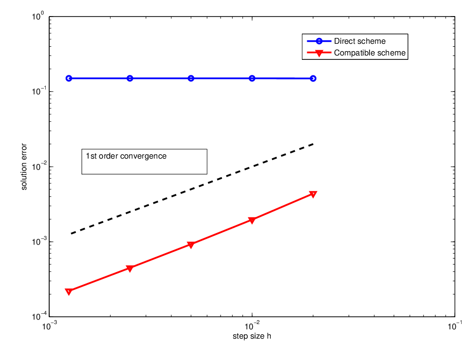
Refer to caption — (a) Solution error vs $h$

Remark 5.2.

For the general case that the interface is at $x^{\ast}\neq 0$ , we have the following formulas in replace of equation (5.2). If $x^{\ast}$ is at the left side of the transitional region, then (5.2) is replace by

\begin{split}\mathcal{L}^{\rm{qnl}}_{\delta}u(x_{i})=&2\int_{x_{i}-x^{\ast}}^{\delta}\gamma_{\delta}(\left|s\right|)\left(u(x_{i}-s)-u(x_{i})\right)ds+2\left(\int_{x_{i}-x^{\ast}}^{\delta}s\gamma_{\delta}(s)ds\right)u^{\prime}(x_{i})\\ +&\left(2\int_{0}^{x_{i}-x^{\ast}}s^{2}\gamma_{\delta}(|s|)ds+2(x_{i}-x^{\ast})\int_{x_{i}-x^{\ast}}^{\delta}s\gamma_{\delta}(|s|)ds\right)u^{\prime\prime}(x_{i})\,.\end{split}

If $x^{\ast}$ is at the right side of the transitional region, then (5.2) is replace by

\begin{split}\mathcal{L}^{\rm{qnl}}_{\delta}u(x_{i})=&2\int_{x^{\ast}-x_{i}}^{\delta}\gamma_{\delta}(\left|s\right|)\left(u(x_{i}+s)-u(x_{i})\right)ds-2\left(\int_{x^{\ast}-x_{i}}^{\delta}s\gamma_{\delta}(s)ds\right)u^{\prime}(x_{i})\\ +&\left(2\int_{0}^{x^{\ast}-x_{i}}s^{2}\gamma_{\delta}(|s|)ds+2(x^{\ast}-x_{i})\int_{x^{\ast}-x_{i}}^{\delta}s\gamma_{\delta}(|s|)ds\right)u^{\prime\prime}(x_{i})\,.\end{split}

5.2. Numerical experiments

We solve the QNL problem (3.5) with right hand side $f$ to be

(5.5)

f(x)=-12x^{2}+4\,.

The exact solution for the limiting local diffusion problem (4.1) is

(5.6)

u_{0}=(1-x)^{2}(1+x)^{2}\quad\text{for }x\in\Omega.

We adopt the discretization scheme described in section 5.1 and compute the QNL solution with the ratio between $\delta$ and spatial step size $h$ to be fixed. Two types of kernels are used with one being $\gamma_{\delta}(x)=\frac{3}{2\delta^{3}}\chi_{(-\delta,\delta)}(x)$ and another being $\gamma_{\delta}(x)=\frac{1}{\delta^{2}|x|}\chi_{(-\delta,\delta)}(x)$ . We compute first the $L^{\infty}$ difference between the QNL solution and the local solution and then the $L^{\infty}$ difference of the gradients which are approximated by second order central finite difference at the mesh points. First order convergences with respect to $h$ are observed in both cases. The results are listed in Table 1 and 2. More careful studies on errors in other norms and more effective gradient recovery techniques, like those proposed in [10] for nonlocal problems, will be studied in the future.

$h$	$\\|u_{\delta}^{\rm{qnl}}-u_{0}\\|_{L^{\infty}}$	Order	$\\|(u_{\delta}^{\rm{qnl}}-u_{0})^{\prime}\\|_{L^{\infty}}$	Order
$1/50$	$1.56e$ - $2$	$-$	$1.91e$ - $2$	$-$
$1/100$	$8.07e$ - $3$	$0.95$	$9.61e$ - $3$	$0.99$
$1/200$	$4.10e$ - $3$	$0.98$	$4.82e$ - $3$	$0.99$
$1/400$	$2.06e$ - $3$	$0.99$	$2.42e$ - $3$	$1.00$
$1/800$	$1.04e$ - $3$	$0.99$	$1.21e$ - $3$	$1.00$

Table 1.

L^{\infty}

differences of solutions

u_{\delta}^{\rm{qnl}}

u_{0}

and their gradients. We fix

\delta=3h

and the kernel function is

\gamma_{\delta}(x)=\frac{3}{2\delta^{3}}\chi_{(-\delta,\delta)}(x)

$h$	$\\|u_{\delta}^{\rm{qnl}}-u_{0}\\|_{L^{\infty}}$	Order	$\\|(u_{\delta}^{\rm{qnl}}-u_{0})^{\prime}\\|_{L^{\infty}}$	Order
$1/50$	$1.19e$ - $2$	$-$	$1.80e$ - $2$	$-$
$1/100$	$6.19e$ - $3$	$0.95$	$9.13e$ - $3$	$0.98$
$1/200$	$3.14e$ - $3$	$0.97$	$4.59e$ - $3$	$0.99$
$1/400$	$1.59e$ - $3$	$0.99$	$2.30e$ - $3$	$1.00$
$1/800$	$7.97e$ - $4$	$0.99$	$1.15e$ - $3$	$1.00$

Table 2.

L^{\infty}

differences of solutions

u_{\delta}^{\rm{qnl}}

u_{0}

and their gradients. We fix

\delta=3h

and the kernel function is

\gamma_{\delta}(x)=\frac{1}{\delta^{2}|x|}\chi_{(-\delta,\delta)}(x)

5.3. Local-nonlocal-local coupling

Volumetric constraints for nonlocal models often cause non-physical boundary layer issues, as shown in Figure 4 $(a)$ . We could fix the boundary layer problem by coupling the nonlocal models with local models and remove the volume constraints completely. Figure 4 $(b)$ shows the solution of the local-nonlocal-local coupling with interfaces at $x^{a}=\frac{-1}{2}$ and $x^{b}=\frac{1}{2}$ . We see that the coupling method removes the artificial boundary layer caused by volume constraints with classical local Dirichlet boundary conditions imposed.

Next we consider the following singular external forces:

(5.7)

f(x)=\frac{(1-x^{2})(1+x^{2})}{|x-x^{*}|},\quad x^{*}=h/2.

The solutions for fully nonlocal, local-nonlocal-local coupling and classical local models are plotted in Figure 5. We can see that the local-nonlocal-local coupling not only captures the singular behavior of the nonlocal solution at $x^{\ast}$ , but also matches with the local solution at two sides of the bar $(-1,1)$ .

6. Conclusion

By extending the idea of “geometric reconstruction” proposed in [12, 20], we developed a top-down quasinonlocal coupling method to study the nonlocal-to-local (NtL) diffusion problem in one dimensional space. This new coupling framework removes interfacial inconsistency and maintains all physical properties at local continuum PDE levels, whereas none of existing coupling methods for nonlocal-to-local problems satisfies all of these properties. We proved the well-posedness of the coupling problem by a quasinonlocal version of the Poincaré inequality and established rigorous estimate of the modeling error by the maximum principle. Furthermore, we proposed a first order finite difference numerical discretization and confirmed the analysis by several numerical tests. The coupling formulation also removes artificial boundary effects caused by the fully nonlocal model when only classical Dirichlet boundary conditions are imposed. Although our discussions here have focused on the scalar one dimensional model problems, it is natural to investigate whether similar ideas can be developed for systems of equations and for problems defined in multi-dimensions. Such generalization is indeed possible, partly because of the fact that the nonlocal diffusion models considered here are based on pairwise interactions, the cases that have been explored in the atomistic-to-continuum coupling methods, see for example [32, 33]. Further investigations will be carried out in our follow-up works along this direction and for nonlocal problems possibly involving more general interactions.

References

[1] E. Askari, F. Bobaru, R. B. Lehoucq, M. L. Parks, S. A. Silling, and O. Weckner. Peridynamics for multiscale materials modeling. Journal of Physics: Conference Series, 125(1), 2008.
[2] P. Bates and A. Chmaj. An integrodifferential model for phase transitions: Stationary solutions in higher space dimensions. Journal of Statistical Physics, 95:1119–1139, 1999.
[3] F. Bobaru and M. Duangpanya. The peridynamic formulation for transient heat conduction. International Journal of Heat and Mass Transfer, 53:4047–4059, 2010.
[4] E. Chasseigne, M. Chaves, and J. D. Rossi. Asymptotic behavior for nonlocal diffusion equations. Journal de Mathématiques Pures et Appliquées, 86:271–291, 2006.
[5] M. D’Elia, M. Perego, P. Bochev, and D. Littlewood. A coupling strategy for nonlocal and local diffusion models with mixed volume constraints and boundary conditions. Computers and Mathematics with applications, 71(11):2218–2230, 2015.
[6] Q. Du, M. Gunzburger, R. Lehoucq, and K. Zhou. Analysis and approximation of nonlocal diffusion problems with volume constraints. SIAM Review, 56:676–696, 2012.
[7] Q. Du, M. Gunzburger, R. Lehoucq, and K. Zhou. A nonlocal vector calculus, nonlocal volume-constrained problems, and nonlocal balance laws. Mathematical Models and Methods in Applied Sciences, 23:493–540, 2013.
[8] Q. Du, R. B. Lehoucq, and A. M. Tartakovsky. Integral approximations to classical diffusion and smoothed particle hydrodynamics. Computer Methods in Applied Mechanics and Engineering, 286:216–229, 2015.
[9] Q. Du and R. Lipton. Peridynamics, fracture, and nonlocal continuum models. SIAM News, 47(3), 2014.
[10] Q. Du, Y. Tao, X. Tian, and J. Yang. Robust a posteriori stress analysis for quadrature collocation approximations of nonlocal models via nonlocal gradients. Computer Methods in Applied Mechanics and Engineering, 310:605–627, 2016.
[11] Q. Du and K. Zhou. Mathematical analysis for the peridynamic nonlocal continuum theory. Mathematical Modelling and Numerical Analysis, 45:217–234, 2010.
[12] W. E, J. Lu, and J. Z. Yang. Uniform accuracy of the quasicontinuum method. Phys. Rev. B, 74(21):214115, 2006.
[13] M. Elices, G. V. Guinea, J. Gómez, and J. Planas. The cohesive zone model: advantages, limitations and challenges. Engineering Fracture Mechanics, 69:137–163.
[14] P. Fife. Some nonclassical trends in parabolic and parabolic-like evolutions. In Trends in Nonlinear Analysis, pages 153–191. Springer, 2003.
[15] W. Gerstle, N. Sau, and S. Silling. Peridynamic modeling of plain and reinforced concrete structures. 18th International Conference on Structural Mechanics in Reactor Technology (SMiRT 18), 2005.
[16] Y. D. Ha and F. Bobaru. Studies of dynamic crack propagation and crack branching with peridynamics. International Journal of Fracture, 162:229–244, 2010.
[17] Y. D. Ha and F. Bobaru. Characteristics of dynamic brittle fracture captured with peridynamics. Engineering Fracture Mechanics, 78:1156–1168, 2011.
[18] F. Han and G. Lubineau. Coupling of nonlocal and local continuum models by the arlequin approach. International Journal for Numerical Methods in Engineering, 89(6):671–685, 2012.
[19] D. Kriventsov. Regularity for a local-nonlocal transmission problem. Archive for Rational Mechanics and Analysis, 217:1103–1195, 2015.
[20] X. H. Li and J. Lu. Quasinonlocal coupling of nonlocal diffusions. 2016. arXiv preprint arXiv:1607.03940.
[21] X. H. Li and M. Luskin. A generalized quasinonlocal atomistic-to-continuum coupling method with finite-range interaction. IMA Journal of Numerical Analysis, 32:373–393, 2011.
[22] R. Lipton. Dynamic brittle fracture as a small horizon limit of peridynamics. Journal of Elasticity, 117:21–50, 2014.
[23] R. Lipton. Cohesive dynamics and brittle fracture. Journal of Elasticity, 124:143–191, 2016.
[24] G. Lubineau, Y. Azdoud, F. Han, C. Rey, and A. Askari. A morphing strategy to couple nonlocal to local continuum mechanics. Journal of the Mechanics and Physics of Solids, 60(6):1088–1102, 2012.
[25] T. Mengesha and Q. Du. The bond-based peridynamic system with dirichlet-type volume constraint. Proceedings of the Royal Society of Edinburgh: Section A Mathematics, 144:161–186, 2014.
[26] P. Ming and J. Z. Yang. Analysis of a one-dimensional nonlocal quasicontinuum method. Multiscale Modeling and Simulation, 7:1838–1875, 2009.
[27] C. Ortner and L. Zhang. Energy-based atomistic-to-continuum coupling without ghost forces. Computer Methods in Applied Mechanics and Engineering, 279:29–45, 2014.
[28] M. L. Parks, R. B. Lehoucq, S. J. Plimpton, and S. Silling. Implementing peridynamics within a molecular dynamics code. Computer Physics Communications, 179:777–783, 2008.
[29] S. Prudhomme, H. Ben Dhia, P. T. Bauman, N. Elkhodja, and J. T. Oden. Computational analysis of modeling error for the coupling of particle and continuum models by the Arlequin method. Computer Methods in Applied Mechanics and Engineering, 197(41-42):3399–3409, 2008.
[30] P. Seleson, S. Beneddine, and S. Prudhomme. A force based coupling scheme for peridynamics and classical elasticity. Computational Materials Science, 66:34–49, 2013.
[31] P. Seleson, Y. D. Ha, and S. Beneddine. Concurrent coupling of bond based peridynamics and the navier equation of classical elasticity by blending. Journal for Multiscale Computational Engineering, 13:91–113, 2015.
[32] A. V. Shapeev. Consistent energy-based atomistic/continuum coupling for two-body potentials in one and two dimensions. Multiscale Modeling and Simulation, 9(3):905–932, 2012.
[33] A. V. Shapeev. Consistent energy-based atomistic/continuum coupling for two-body potentials in three dimensions. SIAM J. Sci. Comput., 34(3):B335–B360, 2012.
[34] T. Shimokawa, J. J. Mortensen, J. Schiotz, and K. W. Jacobsen. Matching conditions in the quasicontinuum method: Removal of the error introduced at the interface between the coarse-grained and fully atomistic region. Phys. Rev. B, 69(21):214104, 2004.
[35] S. Silling. Reformulation of elasticity theory for discontinuities and long-range forces. Journal of the Mechanics and Physics of Solids, 48:175–209, 2000.
[36] S. Silling and R. B. Lehoucq. Peridynamic theory of solid mechanics. Advances in Applied Mechanics, 44:73–168, 2010.
[37] S. Silling, D. J. Littlewood, and P. Seleson. Variable horizon in a peridynamic medium. Journal of Mechancis of Materials and Structures, 10(5):591–612, 2015.
[38] X. Tian. Nonlocal models with a finite range of nonlocal interactions. PhD thesis, Columbia University, 2017.
[39] X. Tian and Q. Du. Analysis and comparison of different approximations to nonlocal diffusion and linear peridynamic equations. SIAM Journal on Numerical Analysis, 51:3458–3482, 2013.
[40] X. Tian and Q. Du. Asymptotically compatible schemes and applications to robust discretization of nonlocal models. SIAM Journal on Numerical Analysis, 52:1641–1665, 2014.
[41] X. Tian and Q. Du. Trace theorems for some nonlocal function spaces with heterogeneous localization. SIAM Journal on Mathematical Analysis, 49(2):1621–1644, 2017.

	$\displaystyle\frac{1}{2}$	$\displaystyle\iint_{x>0\text{ and }y>0}\gamma_{\delta}(\left\|y-x\right\|)\cdot\int_{0}^{1}dt{\left\|u^{\prime}(x+t(y-x))\right\|}^{2}\|y-x\|^{2}$
		$\displaystyle=\frac{1}{2}\int_{0}^{1}dt\int_{x>0}dx\int_{z>(1-t)x}dz\gamma_{\delta}\left(\left\|\frac{z-x}{t}\right\|\right)\|u^{\prime}(z)\|^{2}\frac{1}{t^{3}}\|z-x\|^{2}$
		$\displaystyle=\frac{1}{2}\int_{0}^{1}dt\int_{z>0}dz\|u^{\prime}(z)\|^{2}\int_{0<x<\frac{z}{1-t}}\gamma_{\delta}\left(\left\|\frac{x-z}{t}\right\|\right)\frac{1}{t^{3}}\|x-z\|^{2}~dx$
		$\displaystyle=\frac{1}{2}\int_{z>0}dz\|u^{\prime}(z)\|^{2}\int_{0}^{1}dt\int_{-\frac{z}{t}<s<\frac{z}{1-t}}\gamma_{\delta}\left(\|s\|\right)\|s\|^{2}~ds\,.$

	$\displaystyle\int_{x>0\text{ and }y>0}\gamma_{\delta}(\left\|y-x\right\|)\big(u(y)-u(x)\big)^{2}~dxdy$
	$\displaystyle\quad=\int_{x>0}dx\int_{y>0}dy\gamma_{\delta}(\left\|y-x\right\|)\left[\int_{0<t<1}du\big(x+t(y-x)\big)\right]^{2}$
	$\displaystyle\quad=\int_{x>0}dx\int_{y>0}dy\gamma_{\delta}(\left\|y-x\right\|)\left[\int_{0}^{1}(y-x)\cdot u^{\prime}\big(x+t(y-x)\big)dt\right]^{2}$
(3.3)		$\displaystyle\quad\leq\int_{x>0}dx\int_{y>0}dy\gamma_{\delta}(\left\|y-x\right\|)(y-x)^{2}\int_{0}^{1}\|u^{\prime}\big(x+t(y-x)\big)\|^{2}dt\,,$

	$\displaystyle b^{\rm{qnl}}_{\delta}(u,u)=$	$\displaystyle\int_{x\leq 0\text{ or }y\leq 0}\gamma_{\delta}(\left\|y-x\right\|)\left(u(y)-u(x)\right)^{2}~dxdy+b^{\rm{loc}}_{\delta}(u,u)$
		$\displaystyle\geq\int_{x\leq 0\text{ or }y\leq 0}\gamma_{\delta}(\left\|y-x\right\|)\left(u(y)-u(x)\right)^{2}~dxdy$
		$\displaystyle\qquad+\int_{x>0\text{ and }y>0}\gamma_{\delta}(\left\|y-x\right\|)\big(u(y)-u(x)\big)^{2}~dxdy$

Abstract.

Key words and phrases:

1. Introduction

2. Consistent coupling of nonlocal and local diffusions

2.1. The energy space

Lemma 2.1.

Proof.

Remark 2.1.

Proposition 2.1.

Proof.

Proposition 2.2 (Poincaré inequality).

Proof.

2.2. The QNL operator

Remark 2.2.

2.3. Consistency at the interface

Lemma 2.2.

Proof.

Remark 2.3.

Corollary 2.1 (Patch-test consistency).

Proof.

3. Stability and well-posedness

Lemma 3.1.

Proof.

Proposition 3.1.

Proof.

Theorem 3.1.

Proof.

4. Convergence to the local diffusion as δ→0\delta\to 0

Truncation error

Lemma 4.1 (Maximum principle).

Proof.

Theorem 4.1.

Proof.

5. Numerical discretization and numerical examples

5.1. Numerical scheme

Remark 5.1.

Remark 5.2.

5.2. Numerical experiments

5.3. Local-nonlocal-local coupling

6. Conclusion

References

4. Convergence to the local diffusion as $\delta\to 0$