A New Limit on CMB Circular Polarization from SPIDER
Abstract
We present a new upper limit on CMB circular polarization from the 2015 flight of Spider, a balloon-borne telescope designed to search for -mode linear polarization from cosmic inflation. Although the level of circular polarization in the CMB is predicted to be very small, experimental limits provide a valuable test of the underlying models. By exploiting the non-zero circular-to-linear polarization coupling of the HWP polarization modulators, data from Spider’s 2015 Antarctic flight provide a constraint on Stokes at 95 and 150 GHz from . No other limits exist over this full range of angular scales, and Spider improves upon the previous limit by several orders of magnitude, providing 95% C.L. constraints on ranging from 141 to 255 at 150 GHz for a thermal CMB spectrum. As linear CMB polarization experiments become increasingly sensitive, the techniques described in this paper can be applied to obtain even stronger constraints on circular polarization.
I Introduction
Anisotropies in the intensity and linear polarization of the Cosmic Microwave Background (CMB) have provided a wealth of information about the history and contents of the universe. Standard cosmological models do not predict a measurable amount of circular polarization, characterized by the Stokes parameter, in the CMB; as such, any detection of a primordial signal would be of enormous interest. A variety of secondary physical processes may produce circular polarization in the CMB at very low levels. For instance, Faraday conversion can transform existing linear polarization into circular polarization in both the magnetic fields of galaxy clusters [9] and the relativistic plasma remnants of Population III stars [10]. Magnetic fields in the primordial universe [13, 35], scattering from the cosmic neutrino background [22], and photon-photon interactions in neutral hydrogen [33] have also been shown to potentially produce CMB circular polarization. Additional sources include postulated extensions to QED such as Lorentz-invariance violating operators [8, 2], axion-like pseudoscalar particles [11], and non-linear photon interactions (through effective Euler-Heisenberg Lagrangians) [23]. A brief review of some of these generation mechanisms can be found in King & Lubin [16]. Despite the wide range of physical processes they invoke, all of these mechanisms predict levels of circular polarization that are unlikely to be accessible with current technology.
Nevertheless, circular polarization measurements provide a valuable test of the standard cosmological model and the physics behind these generation mechanisms. Yet there are relatively few published limits. MIPOL reported the strongest constraint on large angular scales () in 2013, providing 95% C.L. measurements ranging from to at 33 GHz [20]. This is roughly an order of magnitude better than the previous 95% C.L. limit of at 33 GHz at [19]. On smaller angular scales, the only reported measurement comes from the VLA, which set 95% C.L. limits at 5 GHz between and for a range of angular scales with [25].
These limits are more than 7 orders of magnitude higher than the best measurements of the linear polarization power spectra, but there are no contemporary experiments with the primary goal of improving them. However, some modern linear polarization experiments, such as Spider, can take advantage of this vast disparity to set stronger limits as a consequence of their polarization modulation techniques.
Spider is a balloon-borne CMB telescope that is searching for a -mode linear polarization signal from cosmic inflation [12, 30]. During its first flight in January 2015, Spider made maps of approximately 10% of the sky with degree-scale angular resolution in 95 and 150 GHz observing bands. The analysis of the linear polarization data from this flight is currently in progress. In this paper, we exploit non-idealities of Spider’s half-wave plate (HWP) polarization modulators to obtain a new upper limit on CMB circular polarization.
The Spider payload features six monochromatic receivers housed in a shared cryostat [15]. Each receiver includes a stepped HWP polarization modulator to reduce the potential impact of systematic errors due to beam asymmetries and instrument polarization [3, 6]. Although Spider’s antenna-coupled TES bolometers are not sensitive to variations in circular polarization [1], non-idealities of the HWPs allow a measurement of the Stokes parameter after combining maps made at several HWP angles. The calculation of Spider’s circular polarization coupling is described in the next section. Section III details how this coupling is used to derive a circular polarization limit. The significance of this result and prospects for future measurements are discussed in Section IV.
II Coupling to Circular Polarization
A birefringent material forms a half-wave plate when the difference in the optical path length between waves polarized along the fast and slow crystal axes is exactly half of the photon wavelength. An ideal HWP rotates the polarization plane of the light passing through it by , where is the angle between the incoming polarization plane and the slow crystal axis. However, this condition can only be exactly satisfied at a single frequency. Similarly, the single-layer anti-reflection (AR) coatings applied to Spider’s HWPs are not uniformly efficient over the observing bands. When combined, these conditions lead to a frequency-dependent reduction in transmission through the HWPs and induce non-ideal polarization modulation effects as the HWPs are rotated. Since Spider’s observing bands have roughly 20% bandwidths, the magnitude of such effects could be significant.
Following Bryan et al. [5], a non-ideal HWP can be modeled with four parameters that can be broadly interpreted as the total transmission , the difference in transmission between the fast and slow axes , the linear polarization response , and the coupling to circular polarization . In terms of these parameters, the Mueller matrix of a HWP with its birefringent crystal axes oriented along the horizontal and vertical directions can be written as
| (1) |
For an ideal HWP, , , and . The ideal case captures the effect of the HWP on linear polarization signals and has no coupling between linear and circular polarization (). In real HWPs, however, these parameters can deviate significantly from their ideal values. While simulations have shown that these non-idealities are not problematic for detecting a -mode signal at Spider’s anticipated sensitivity level [24], they allow Spider to measure circular polarization to the extent that is non-zero.
The sky signal in a detector timestream is given in terms of the Stokes parameters , , , and and the instrument Mueller matrix elements by
| (2) |
The instrument Mueller matrix is calculated in Bryan et al. [5] by multiplying the Mueller matrices of every element in the optical chain, including from Equation 1. For the purposes of this paper we are interested only in the instrument Mueller matrix element . Generalizing the treatment in Bryan et al. [5] for arbitrary detector angles, it is straightforward to show that the parameter couples to a detector timestream as
| (3) |
Here is the HWP angle and is the detector angle, both of which are defined relative to the instrument. Note that does not depend on the rotational orientation of the instrument relative to the sky and can be positive, negative, or zero depending on the relative HWP and detector angles. The overall polarization efficiency of the instrument is described by , while describes the coupling to circular polarization from the HWP non-idealities. Note that does not appear in the , , or matrix elements in Equation 2 and therefore is not used in Spider’s linear polarization analysis.
| 95 GHz Receivers | X2 | X4 | X6 |
|---|---|---|---|
| Sapphire (mm) | 4.97 0.01 | 4.94 0.01 | 4.97 0.01 |
| Top Quartz Layer (mm) | 0.420 0.015 | 0.429 0.015 | 0.427 0.015 |
| Bottom Quartz Layer (mm) | 0.419 0.015 | 0.419 0.015 | 0.422 0.015 |
| Gap (mm) | 0.01 0.01 | 0.01 0.01 | 0.01 0.01 |
| 150 GHz Receivers | X1 | X3 | X5 |
|---|---|---|---|
| Sapphire (mm) | 3.21 0.01 | 3.26 0.01 | 3.23 0.01 |
| Top Cirlex Layer (mm) | 0.250 0.005 | 0.250 0.005 | 0.250 0.005 |
| Bottom Cirlex Layer (mm) | 0.250 0.005 | 0.250 0.005 | 0.250 0.005 |
| HDPE Bond Layer (mm) | 0.006 0.001 | 0.006 0.001 | 0.006 0.001 |
| Material | Refractive Index () | Reference |
|---|---|---|
| Sapphire (fast axis) | 3.019 0.003 | Bryan et al. [4] |
| Sapphire (slow axis) | 3.336 0.003 | Bryan et al. [4] |
| Quartz (fused) | 1.95 0.01 | Bryan [3] |
| Cirlex | 1.94 0.01 | Bryan [3] |
| HDPE | 1.56 0.01 | Lamb [17] |
Spider’s six receivers are assigned names consisting of the letter ‘X’ followed by the numbers 1 through 6, where the even numbers refer to 95 GHz receivers and the odd numbers to 150 GHz receivers. Each receiver has a dedicated HWP and therefore a unique value of the non-ideality parameter. It can be calculated as described in Bryan et al. [5] from the thicknesses and refractive indices of the HWP materials, the spectrum of the observed source, and the shape of the observing band. Similar HWP modeling techniques have been used for the linear polarization properties of sapphire HWPs by Savini et al. [32] and found to be in good agreement with experimental measurements [26, 31, 3].
For the results presented in this paper, uncertainties in the component properties lead to significant uncertainty in for each HWP, which is quantified with Monte Carlo simulations. We use the temperature derivative of the CMB blackbody spectrum for the source in the baseline case, as well as the thicknesses and uncertainties of the HWP components listed in Tables 1 and 2, and the refractive indices and uncertainties of the materials in Table 3. Since the refractive indices of sapphire should be the same for every HWP, we use the same randomly drawn values of the two indices for all receivers in each iteration of the calculations.
To take Spider’s observing bands into account, we use Fourier Transform Spectrometer (FTS) measurements made just prior to flight [14]. However, correctly interpreting these measurements relies on knowing the frequency dependence of the coupling to the Rayleigh-Jeans calibration source. Although the intensity of the source has a frequency dependence, the beam throughput () scales as in the beam-filling limit. For Spider, the source is not entirely beam filling, and calculations indicate that this coupling should be approximately . This leads to larger absolute values of than in the beam-filling case. However, due to the relatively large uncertainty in the calculation of this scaling, we adopt a conservative approach in this paper and assume a coupling, likely underestimating .
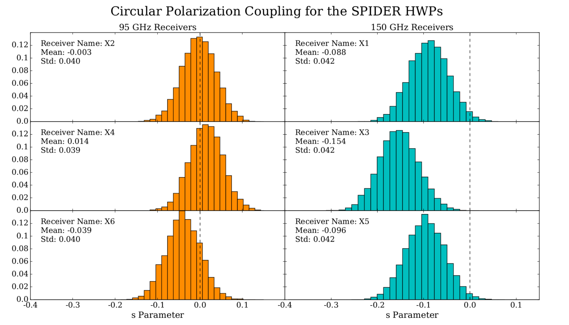
The probability distributions of the parameters for a CMB source for each Spider receiver are shown in Figure 1. These are derived from 10,000 Monte Carlo simulations, which calculate a new value of for each iteration following the methodology presented by Bryan et al. [5], using randomly drawn sets of physical parameters based on the central values and uncertainties listed in Tables 1-3. The distributions of for the 150 GHz systems exclude zero at roughly 2- to 4-. At 95 GHz, they include within the 1- range. However, to the extent that these distributions are truly good estimators of the probability distributions, they can still be used to constrain the amplitude of circular polarization by virtue of the significant probability of non-zero . Note that having three separate HWPs at each frequency greatly improves Spider’s statistical power to constrain . The differences in distributions between receivers at the same frequency are caused by differences in the shapes of the measured observing bands for each receiver and in the measured thicknesses of the actual HWP components.
III Results
During the 2015 flight, Spider observed approximately 4500 square degrees of sky near the southern Galactic pole, centered around roughly RA=50∘ and Dec=-35∘. For the first 7.5 days used in this analysis, almost the entire region was mapped every 12 sidereal hours following a sinusoidal azimuth scan profile and using a scan width of 70∘ peak-to-peak. Maps for the remaining 4.5 days covered smaller overlapping sub-regions using narrower sinusoidal azimuth scans with widths of 35∘ peak-to-peak [34]. The HWPs were held at fixed angles during each of these maps and rotated to new angles between them, following the patterns shown in Figure 2. Over the course of the flight, each receiver observed the sky at 8 discrete HWP angles nominally spaced at 22.5 degree intervals.
The data from individual receivers are combined into 4 independent sets, illustrated by the colored bands in Figure 2, which were optimized for separating the , , and signals. Each of these sets is used to construct an independent map with a binned map-maker [29], using the values of polarization efficiency listed in Table 4. If the value for each receiver was known exactly, Equations 2 and 3 could be used by the mapmaker to construct maps directly from the Spider data. Instead, since the values of actually follow broad probability distributions, and appears only in the matrix element in Equation 2, we make maps assuming and later scale the resulting power spectra.
| Receiver Name | Frequency | Polarization Efficiency () |
|---|---|---|
| X1 | 150 GHz | 0.959 0.005 |
| X2 | 95 GHz | 0.965 0.001 |
| X3 | 150 GHz | 0.950 0.008 |
| X4 | 95 GHz | 0.964 0.001 |
| X5 | 150 GHz | 0.956 0.005 |
| X6 | 95 GHz | 0.964 0.003 |
Before making these maps, glitches such as cosmic ray hits, payload transmitter signals, and thermal transients are identified and removed from the detector timestreams. This pipeline is shared with the linear polarization analysis and will be described more extensively in a future publication. Some detectors have been excluded from this analysis due to undesirable remaining timestream features, but a number of them may be recovered for future results. Here we use 681 detectors at 95 GHz and 1117 detectors at 150 GHz, rejecting an average of approximately 30% of the data from these timestreams. For this result we subtract a fifth-order polynomial fit in azimuth from each scan (approximately 30 seconds of data) to remove scan-synchronous noise.
Only part of Spider’s observing region is used for the circular polarization analysis, masking data outside of and . The leakage from other signals to is subtracted in map-space from full timestream signal simulations based on Planck 100 and 143 GHz temperature-only input maps [27]. This is dominated by -to- leakage from the polynomial timestream filter, which is at the level of in the original maps and roughly 2 orders of magnitude smaller than our sensitivity. The -to- leakage is about 5 orders of magnitude lower. The pipeline was verified through simulations in which an input signal-only map was observed following Spider’s scan strategy and then recovered after applying the same flagging and filtering to the re-observed timestreams.
The cross-spectra of the maps are estimated with PolSpice [7], which takes the sky mask into account. We apply a transfer function to account for the effects of timestream filtering and beam smoothing, where the beam correction is derived from map-domain fits to Planck temperature maps. The transfer function is obtained by comparing spectra from smoothed Planck maps of the Spider region to spectra from simulated re-observations of those Planck maps that include Spider’s pointing and timestream filtering.
The cross-spectra for pairs of maps at a given frequency are then combined with Monte Carlo simulations. In each iteration, values of for receivers and are drawn from the distributions shown in Figure 1, and the cross-spectra are then scaled by . Note that the selected values are slightly correlated due to the common sapphire indices. We calculate the weighted mean of the resulting values in each bin, weighting by the variance of the map cross-spectra in that bin. This process is repeated 10,000 times, and the mean and error in each bin are derived from the resulting distribution.
At 150 GHz we cross every pair of maps from each of the three receivers and four independent sets, excluding the auto-spectra, for a total of 66 cross-spectra. This includes crossing maps made simultaneously on different receivers because the noise has been shown to be no more correlated than in any of the other map pairs. At 95 GHz we only cross maps from the same receiver because the distributions allow both positive and negative values with significant probabilities. A sign error on either or (but not both) relative to the true value would flip the sign of the cross-spectrum, potentially suppressing real signals upon averaging. By restricting ourselves to the 18 cross-spectra that can be constructed from single-receiver maps, we ensure that is always positive, thus avoiding this problem at the price of a small noise penalty.
| Bin Center () | 95 GHz Limit () | 150 GHz Limit () |
| 45 | 1088 | 195 |
| 70 | 783 | 153 |
| 95 | 842 | 149 |
| 120 | 853 | 141 |
| 145 | 856 | 142 |
| 170 | 985 | 164 |
| 195 | 1032 | 177 |
| 220 | 1129 | 197 |
| 245 | 1254 | 242 |
| 270 | 1455 | 244 |
| 295 | 1760 | 255 |
Figure 3 shows Spider’s CMB spectra at 95 and 150 GHz, neither of which indicate a significant detection of circular polarization. The mean values and errors are derived from the distributions of the -scaled cross-spectra, and the spread in each of those distributions has contributions from both the distribution of the various cross-spectra and the distributions of values. Figure 4 shows the 95% C.L. limits on CMB circular polarization derived from these spectra, and the numerical values are provided in Table 5. Although the measurements are made at different frequencies, they are expressed in units of CMB temperature, which are the equivalent fluctuations of a 2.73 K blackbody required to produce the measured intensity variations. This result represents an improvement of several orders of magnitude over the previous best upper limit [20] at a complementary range of angular scales.
However, Spider’s limits depend on the chosen source spectrum through the calculations of the HWP coupling parameters . Many of the methods for generating CMB circular polarization described in Section I predict polarization signals with spectra of the form or . We therefore recalculate Spider’s distributions for such source spectra and find that the limits in Figure 4 typically become lower. Still expressed in CMB temperature units, they scale by factors of 0.39 and 0.10 respectively at 95 GHz and 1.02 and 0.30 respectively at 150 GHz. In all of these cases, Spider’s circular polarization limits are still many orders of magnitude above the predicted cosmological signals.
Similarly, the limits presented in this paper can also be extended to upper limits on foreground circular polarization by recomputing with the appropriate source spectra. King & Lubin [16] suggest that is a reasonable model for synchrotron circular polarization. With this source spectrum, Spider’s circular polarization limits in Figure 4 scale by 0.08 at 95 GHz and 0.11 at 150 GHz, still using CMB temperature units. To obtain an estimate of Spider’s limit on the circular polarization of thermal dust, we use the linear polarization model of for the source spectrum [28] since we are not aware of any circularly polarized dust models. This leads to circular polarization limits that scale from Figure 4 by 0.27 at 95 GHz and 0.56 at 150 GHz. Although these models of the source spectra are relatively uncertain, the predicted foreground signals are many orders of magnitude below Spider’s sensitivity level.
IV Conclusion
This paper presents a new upper limit on CMB circular polarization from at 95 and 150 GHz. It was obtained by exploiting a non-ideality of the HWP polarization modulators used by Spider to measure linear polarization during a 2015 Antarctic flight. This represents an improvement of several orders of magnitude over the previous limit, providing 95% C.L. constraints on ranging from 141 to 255 at 150 GHz for a thermal CMB spectrum. When recalculated for and source spectra, this limit scales by 1.02 and 0.30 respectively. Data from Spider’s second flight, planned for December 2018, could provide increased sensitivity at 95 and 150 GHz as well as a new measurement at 280 GHz over the same range of angular scales.
As linear polarization experiments become increasingly sensitive, the techniques described in this paper can be applied to provide stronger constraints on CMB circular polarization. Several current and planned experiments use either HWPs or Variable-delay Polarization Modulators (VPMs) [21], both of which can be used to measure . Although the current limit is many orders of magnitude larger than the most optimistic signal predictions, these measurements provide an observational test of the standard cosmological model and a wide range of physical processes. Since this limit is still about four orders of magnitude above modern linear polarization measurements, a dedicated experiment with better -coupling could make significant improvements using existing technology.
References
- [1] Ade, P. A. R., Aikin, R. W., Amiri, M., et al. 2015, The Astrophysical Journal, 812, 176
- [2] Alexander, S., Ochoa, J., & Kosowsky, A. 2009, Physical Review D, 79, 063524
- [3] Bryan, S. A. 2014, Half-Wave Plates for the SPIDER Cosmic Microwave Background Polarimeter (PhD thesis, Case Western Reserve University)
- [4] Bryan, S. A., Ade, P. A. R., Amiri, M., et al. 2010a, in SPIE Astronomical Telescopes+ Instrumentation, Vol. 7741, Society of Photo-Optical Instrumentation Engineers
- [5] Bryan, S. A., Montroy, T. E., & Ruhl, J. E. 2010b, Applied Optics, 49, 6313
- [6] Bryan, S. A., Ade, P. A. R., Amiri, M., et al. 2016, Review of Scientific Instruments, 87, 014501
- [7] Chon, G., Challinor, A., Prunet, S., Hivon, E., & Szapudi, I. 2004, Monthly Notices of the Royal Astronomical Society, 350, 914
- [8] Colladay, D., & Kosteleckỳ, V. A. 1998, Physical Review D, 58, 116002
- [9] Cooray, A., Melchiorri, A., & Silk, J. 2003, Physics Letters B, 554, 1
- [10] De, S., & Tashiro, H. 2015, Physical Review D, 92, 123506
- [11] Finelli, F., & Galaverni, M. 2009, Physical Review D, 79, 063002
- [12] Fraisse, A. A., Ade, P. A. R., Amiri, M., et al. 2013, Journal of Cosmology and Astroparticle Physics, 2013, 047
- [13] Giovannini, M. 2009, Physical Review D, 80, 123013
- [14] Gudmundsson, J. E. 2014, Probing Early Universe Cosmologies with SPIDER & Planck HFI (PhD thesis, Princeton University)
- [15] Gudmundsson, J. E., Ade, P. A. R., Amiri, M., et al. 2015, Cryogenics, 72, 65
- [16] King, S., & Lubin, P. 2016, Physical Review D, 94, 023501
- [17] Lamb, J. W. 1996, International Journal of Infrared and Millimeter Waves, 17, 1997
- [18] Loken, C., Gruner, D., Groer, L., et al. 2010, in Journal of Physics: Conference Series, Vol. 256, IOP Publishing, 012026
- [19] Lubin, P., Melese, P., & Smoot, G. 1983, The Astrophysical Journal, 273, L51
- [20] Mainini, R., Minelli, D., Gervasi, M., et al. 2013, Journal of Cosmology and Astroparticle Physics, 2013, 033
- [21] Miller, N. J., Chuss, D. T., Marriage, T. A., et al. 2016, The Astrophysical Journal, 818, 151
- [22] Mohammadi, R. 2014, The European Physical Journal C, 74, 3102
- [23] Motie, I., & Xue, S.-S. 2012, Europhysics Letters, 100, 17006
- [24] O’Dea, D. T., Ade, P. A. R., Amiri, M., et al. 2011, The Astrophysical Journal, 738, 63
- [25] Partridge, R., Nowakowski, J., & Martin, H. 1988, Nature, 331, 146
- [26] Pisano, G., Savini, G., Ade, P. A., Haynes, V., & Gear, W. K. 2006, Applied Optics, 45, 6982
- [27] Planck Collaboration. 2016a, Astronomy & Astrophysics, 594, A1
- [28] —. 2016b, Astronomy & Astrophysics, 594, A10
- [29] Rahlin, A. S. 2016, The First Flight Of The SPIDER Balloon-Borne Telescope (PhD thesis, Princeton University)
- [30] Rahlin, A. S., Ade, P. A. R., Amiri, M., et al. 2014, in SPIE Astronomical Telescopes+ Instrumentation, International Society for Optics and Photonics, 915313–915313
- [31] Savini, G., Ade, P. A., House, J., et al. 2009, Applied Optics, 48, 2006
- [32] Savini, G., Pisano, G., & Ade, P. A. 2006, Applied Optics, 45, 8907
- [33] Sawyer, R. 2015, Physical Review D, 91, 021301
- [34] Shariff, J. A. 2015, Polarimetry from the Stratosphere with SPIDER and BLASTPol (PhD thesis, University of Toronto)
- [35] Zarei, M., Bavarsad, E., Haghighat, M., et al. 2010, Physical Review D, 81, 084035