Numerical calculation of the decay widths, the decay constants, and the decay energy spectra of the resonances of the delta-shell potential

Although there are several theoretical ways to describe a resonance, there is increasing evidence in molecular, atomic, nuclear and particle physics that a resonance should be defined as a pole of the $S$ matrix [1], due to the phenomenological and theoretical advantages of such definition [2, 3, 4, 5, 6, 7, 8, 9, 12, 10, 11, 13, 14, 15, 16, 17, 18, 19]. Once we accept the definition of a resonance as a pole of the $S$-matrix, it is very natural to associate with it a resonant (Gamow) state [20, 21, 22, 23, 24, 25, 26, 27, 28, 29, 30, 31, 32, 33, 34, 35, 36, 37, 38, 39, 40, 41, 42, 43, 44, 45, 46, 47, 48, 49, 50, 51, 52, 53, 55, 54, 56].

Because resonant states are the wave functions of resonances, it is logical to obtain from them measurable quantities such as decay rates and branching fractions. In Ref. [48], it was shown how to construct the decay energy spectrum, the differential and the total decay widths, and the differential and the total decay constants of a resonant state. In the present paper, we will use the example of the delta-shell potential to obtain a numerical validation of the results of Ref. [48]. Such numerical validation is needed because there is a result of perturbation theory [57] that is seemingly in conflict with the results of Ref. [48]. The explicit numerical calculation of the quantities introduced in Ref. [48] will show that the formalism of Ref. [48] is indeed sound.

Although it is not very realistic, the delta-shell potential [59, 58, 60] is frequently used to exemplify and test new results in the theory of resonances, because it is the simplest potential that produces resonances, and because it is almost exactly solvable. For example, in Ref [27], a double delta-shell potential was used to numerically obtain an exceptional point. In Ref. [37], the delta-shell potential was utilized to study the decay of two identical, non-interacting particles. In Ref. [38], it was used to illustrate that the resonant states yield the same time evolution of a wave packet as the scattering states. In Refs. [39, 44], the delta-shell potential with a complex coupling was employed to study time evolution in the presence of absorbing and emitting potentials. In Ref. [56], it was used to study the non-Hermitian character of the Born rule in open quantum systems. In Ref. [61], a double well Dirac delta function model was utilized as the one-dimensional limit of H${}_{2}^{+}$. In Ref. [62], the delta-shell potential was used to relate resonances with the eigenstates of a particle in a box by means of renormalization and mixing. In Ref. [63], it was utilized to study perturbative and non-perturbative dynamics of resonances. In our case, besides its simplicity, we use the delta-shell potential because we have found that the transcendental equation that provides its resonant energies can actually be solved exactly in terms of the Lambert $W$ function, thereby making the delta-shell potential a fully solvable model for resonances.

It is important to understand to what kind of situations the decay energy spectrum of Ref. [48] would apply. Resonances appear as sharp peaks of the cross section. For example, in the reaction $\pi^{+}+p\to\pi^{+}+p$, there is a sharp peak centered at 1230 MeV whose width is about 115 MeV [64]. Such peaks are thought to be due to intermediate, unstable particles that are described by a pole of the $S$-matrix, and they are interpreted in terms of the cross section rather than the decay energy spectrum of Ref. [48]. Resonances are also observed when the energy spectrum of its decay products is measured. For example, in the reaction $\pi^{+}+p\to\pi^{+}+\pi^{0}+p$, we can plot the number of decay evens of $\pi^{+}\pi^{0}$ versus the invariant mass of the two pions [64]. It is then found that there is a peak around 770 MeV that corresponds to the energy of the $\rho^{+}$ resonance. The reaction is then thought to proceed in two steps. In the first one, a proton and the $\rho^{+}$ are produced; in the second one, the $\rho^{+}$ decays into two pions. It is to this kind of situations –when the decay energy spectrum of a resonance is measured by counting the number of decay products as a function of the energy– that the decay energy spectrum of Ref. [48] applies, in the non-relativistic domain.

Our results are based on the assumption that the wave function of a resonance is exactly given by a resonant state. However, a recurring objection to the use of resonant states is that such states are not physical. In order to counter such objection, we would like to point out that, theoretically, using a resonant state to describe a resonance is complementary to, and in the same spirit as, using a pole of the $S$-matrix. When one describes a resonance as the pole of the $S$-matrix (which is defined on the scattering spectrum), one analytically continues the $S$-matrix from the real, scattering energies (which are the only energies that are accessible by experiment), to the complex resonant pole (which is not directly accessible by experiment). The Laurent expansion of the $S$-matrix is the sum of a resonant part (the pole’s contribution), and a non-resonant part (the background). The $S$-matrix description of a resonance assumes that the resonance’s contribution to the cross section is given by the pole’s contribution, and that the background has nothing to do with the resonance itself. Similarly, when one uses a wave function $\varphi$ to describe a system with resonances, one analytically continues $\varphi$ from the real, scattering energies into the complex pole of the $S$-matrix, resulting in an expansion of the form $|\varphi\rangle=c_{\text{\tiny R}}|z_{\text{\tiny R}}\rangle+|\text{bg}\rangle$. In such expansion, the resonant state $|z_{\text{\tiny R}}\rangle$ is supposed to carry the resonance’s contribution to the state $\varphi$ (including the exponential decay), and the background $|\text{bg}\rangle$ is supposed to carry the non-resonant contributions (including deviations from exponential decay).

Since one can use the formalism of Ref. [48] to calculate the decay rate of a square-integrable wave function $\varphi$, one may be tempted to identify the decay rate of a wisely chosen $\varphi$, rather than the decay rate of a resonant state, with the true decay rate of a resonance. However, describing the decay rate of a resonance by way of a square-integrable function $\varphi$ leads to ambiguities. To see why, let us imagine that we are using a wave function $\varphi_{1}$ to obtain the decay rate and the lifetime of a resonance. We can always expand $\varphi_{1}$ in terms of the resonant state, $\varphi_{1}=c_{\text{\tiny R,1}}|{z_{\text{\tiny R}}}\rangle+|\text{bg}_{1}\rangle$. But if we used a wave function $\varphi_{2}=c_{\text{\tiny R,2}}|z_{\text{\tiny R}}\rangle+|\text{bg}_{2}\rangle$ that is only slightly different from $\varphi_{1}$, we would obtain a slightly different decay rate and a slightly different lifetime, and we could not tell which ones are the right ones, let alone relate them to the pole width. The Gamow-state description of resonances addresses this ambiguity by associating a unique Gamow state to each pole of the $S$-matrix, and by defining resonant properties such as decay rates and lifetimes in terms of the Gamow states. In our example, there is only one resonance, and $\varphi_{1}$ and $\varphi_{2}$ are two different approximations of one and the same resonant state. The backgrounds $|\text{bg}_{1}\rangle$ and $|\text{bg}_{2}\rangle$ provide a measure of how well the wave function is tuned around the resonant state. Thus, by identifying the resonant state with the wave function of a resonance, one has an unambiguous way to prescribe what is resonance from what is background.

Since we will denote similar quantities by similar symbols, it may be helpful to review our notation. The differential and the total decay widths will be denoted by $\frac{{\rm d}\overline{\Gamma}(E)}{{\rm d}E}$ and $\overline{\Gamma}$, respectively. The differential and the total decay constants will be denoted by $\frac{{\rm d}\Gamma(E)}{{\rm d}E}$ and $\Gamma$, respectively. The complex, resonant energy, which is a pole of the $S$ matrix, will be denoted by $z_{\text{\tiny R}}=E_{\text{\tiny R}}-{\rm i}\Gamma_{\text{\tiny R}}/2$, where $E_{\text{\tiny R}}$ is the (mean) energy of the resonant state, and $\Gamma_{\text{\tiny R}}$ is the pole width.

The structure of the paper is as follows. In Sec. 2, we review the main properties of the delta-shell potential and obtain the resonant energies for the zero angular momentum case. We will show that the transcendental equation that provides the resonant energies can be solved explicitly in terms of the Lambert $W$ function. In Sec. 3, we calculate the decay widths $\overline{\Gamma}$ and the decay constants $\Gamma$. We will show that the closer the resonance is to the real axis (and hence the closer it is to become a bound state), the smaller $\overline{\Gamma}$ is, and the larger $\Gamma$ is. Thus, both $\overline{\Gamma}$ and $\Gamma$ can be used to quantify the strength of the interaction between the resonance and the continuum. We will also point out that, although a standard result of perturbation theory seems to be in contradiction with the formalism of Ref. [48], the numerical results of the present paper show that such formalism is well grounded. In Sec. 4, we use the Golden Rule of a resonant state to obtain the values of the decay widths and constants in the approximation that the resonance is sharp. We will denote such approximate values by $\overline{\Gamma}_{\rm sharp}$ and $\Gamma_{\rm sharp}$. We will show that, surprisingly, for truly sharp resonances $\overline{\Gamma}_{\rm sharp}$ is very close to the pole width $\Gamma_{\text{\tiny R}}$, even though $\overline{\Gamma}$ is very different from $\Gamma_{\text{\tiny R}}$. In Sec. 5, we obtain the theoretical probability $\frac{{\rm d}P(E)}{{\rm d}E}$ that is to correspond to the experimental decay energy spectrum. We will show numerically that the Breit-Wigner (Lorentzian) distribution does not coincide exactly with the natural lineshape of a resonance, even when the effect of the threshold can be neglected. In addition, we will show that $\frac{{\rm d}P(E)}{{\rm d}E}$ naturally suggests a new normalization of the resonant states. We will also point out some similarities of the decay energy spectra of the delta-shell potential with experimental ones. In Sec. 6, we obtain the decay energy spectrum of two interfering resonances, and we argue that the standard Golden Rule is not suitable to describe such interference. Although cross sections are not the main focus of the present paper, in Sec. 7 we compare three different approximations of the $S$-matrix to describe resonant peaks in cross sections. Finally, in Sec. 8 we state our conclusions.

Let us review the main features of the delta-shell potential [59]. A delta-shell potential at $r=a$ is given by

$$V(r)=g\delta(r-a)\,,$$

(2.1)

where $g$ characterizes the opaqueness of the barrier. In the radial, position representation, and for zero angular momentum, the eigensolutions of the time-independent Schrödinger equation subject to appropriate boundary conditions are given by

$$\chi(r;E)=A(E)\left\{\begin{array}[]{ll}\sin(kr)&0<r<a\,,\\[8.61108pt] {\cal J}_{1}(E){\rm e}^{{\rm i}kr}+{\cal J}_{2}(E){\rm e}^{-{\rm i}kr}&a<r<\infty\,,\end{array}\right.$$

(2.2)

where $k=\sqrt{\frac{2m}{\hbar^{2}}E}$ is the wave number, $A(E)$ is a normalization constant, and the Jost functions are given by

$${\cal J}_{{\,}{}_{2}^{1}}(E)=\frac{1}{4k}\left[\mp 2{\rm i}k+\frac{2mg}{\hbar^{2}}\left({\rm e}^{\mp 2{\rm i}ka}-1\right)\right]\,.$$

(2.3)

The $S$-matrix is given by

$$S(E)=-\frac{{\cal J}_{1}(E)}{{\cal J}_{2}(E)}\,.$$

(2.4)

The resonant wave numbers are given by the poles of the $S$-matrix, which coincide with the zeros of ${\cal J}_{2}(E)$,

$$2{\rm i}ka+\lambda\left({\rm e}^{2{\rm i}ka}-1\right)=0\,,$$

(2.5)

where $\lambda=\frac{2m}{\hbar^{2}}ga$ is a dimensionless constant that characterizes the strength of the potential. Equation (2.5) is a transcendental equation that has an infinite number of complex solutions. Such solutions can be written in terms of the Lambert $W$ function [65, 66, 67, 68, 69, 70, 71]. The resonant wave numbers, which lie in the fourth quadrant, are given by

$$k_{n}\equiv\alpha_{n}-{\rm i}\beta_{n}=\left\{\begin{array}[]{lc}\frac{1}{2{\rm i}a}\left[\lambda-W_{-n}(\lambda{\rm e}^{\lambda})\right]\,,&n=1,2,\ldots,\quad\lambda>0\,,\\[8.61108pt] \frac{1}{2{\rm i}a}\left[\lambda-W_{-n}(\lambda{\rm e}^{\lambda})\right]\,,&n=2,3,\ldots,\quad\lambda<0\,,\end{array}\right.$$

(2.6)

where $W_{n}$ is the $n$th branch of the Lambert $W$ function. For $\lambda<-1$, the delta-shell potential forms a bound state whose wave number is given by

$$k_{\rm b}\equiv{\rm i}|k_{\rm b}|=\frac{1}{2{\rm i}a}\left[\lambda-W_{0}(\lambda{\rm e}^{\lambda})\right]\,.$$

(2.7)

For $-1<\lambda<0$, the delta-shell potential forms a virtual (also known as anti-bound) state of wave number

$$k_{\rm v}\equiv-{\rm i}|k_{\rm v}|=\frac{1}{2{\rm i}a}\left[\lambda-W_{-1}(\lambda{\rm e}^{\lambda})\right]\,.$$

(2.8)

For any $\lambda$, the anti-resonant wave numbers, which lie in the third quadrant, are given by

$$k_{-n}\equiv-\alpha_{n}-{\rm i}\beta_{n}=-k_{n}^{*}=\frac{1}{2{\rm i}a}\left[\lambda-W_{n}(\lambda{\rm e}^{\lambda})\right]\,,\qquad n=1,2,\ldots\,.$$

(2.9)

By using a program such as Mathematica, Maple or Matlab, it is very easy to calculate the resonant wave numbers of the delta-shell potential for a given value of $\lambda$. Tables 1-6 in Appendix B list the first eight resonant wave numbers and energies for the cases $\lambda=\pm 0.5,\pm 10,$ and $\pm 100$ in units where $a=\hbar^{2}/2m=1$. This choice of units is equivalent to measuring wave number in units of $1/a$ and energy in units of $\hbar^{2}/2ma^{2}$. The virtual ($\lambda=-0.5$, Table 4) and bound ($\lambda=-10$, Table 5; $\lambda=-100$, Table 6) states are also listed.

The resonant eigenfunctions are given by

$$\langle r|z_{\text{\tiny R}}\rangle=u(r;z_{\text{\tiny R}})=N_{\text{\tiny R}}\left\{\begin{array}[]{ll}\frac{1}{{\cal J}_{1}(z_{\text{\tiny R}})}\sin(k_{\text{\tiny R}}r)&0<r<a\,,\\[8.61108pt] {\rm e}^{{\rm i}k_{\text{\tiny R}}r}&a<r<\infty\,,\end{array}\right.$$

(2.10)

where Zeldovich’s normalization constant $N_{\text{\tiny R}}$ is given by the residue of the $S$-matrix at the complex resonant wave number $k_{\text{\tiny R}}$,

$$N_{\text{\tiny R}}^{2}={\rm i}\,\text{res}\left[S(q)\right]_{q=k_{\text{\tiny R}}}=-{\rm i}\,\frac{{\cal J}_{1}(k_{\text{\tiny R}})}{{\cal J}_{2}^{\prime}(k_{\text{\tiny R}})}\,.$$

(2.11)

In Ref. [48], we identified $|\langle E|{\rm e}^{-{\rm i}H\tau/\hbar}|z_{\text{\tiny R}}\rangle|^{2}$ with the probability density $\frac{{\rm d}p_{\tau}}{{\rm d}E}$ that the resonance has decayed into a stable particle of energy $E$ at time $\tau$,

$$\frac{{\rm d}p_{\tau}}{{\rm d}E}\equiv|\langle E|{\rm e}^{-{\rm i}H\tau/\hbar}|z_{\text{\tiny R}}\rangle|^{2}\,.$$

(3.1)

The differential decay width associated with such a probability is defined as (see Refs. [72, 73] for a somewhat related definition)

$$\frac{{\rm d}\overline{\Gamma}(E)}{{\rm d}E}\equiv-\hbar\frac{{\rm d}}{{\rm d}\tau}\left(\left.\frac{{\rm d}p_{\tau}}{{\rm d}E}\right)\right|_{\tau=0}\,.$$

(3.2)

As shown in Ref. [48], the differential and the total decay widths of a resonant state can be written as

	$\displaystyle\frac{{\rm d}\overline{\Gamma}(E)}{{\rm d}E}=\frac{\Gamma_{\text{\tiny R}}}{(E-E_{\text{\tiny R}})^{2}+(\Gamma_{\text{\tiny R}}/2)^{2}}|\langle E|V|z_{\text{\tiny R}}\rangle|^{2}\,,$		(3.3)
	$\displaystyle\overline{\Gamma}=\int_{0}^{\infty}{\rm d}E\ \frac{\Gamma_{\text{\tiny R}}}{(E-E_{\text{\tiny R}})^{2}+(\Gamma_{\text{\tiny R}}/2)^{2}}|\langle E|V|z_{\text{\tiny R}}\rangle|^{2}\,.$		(3.4)

The decay width $\overline{\Gamma}$ has units of energy, and physically can be interpreted as the initial decay rate associated with the probability $p_{\tau}$. Thus, at least in principle, one could measure $\overline{\Gamma}$ by measuring the initial decay rate of $p_{\tau}$. However, in general $\overline{\Gamma}$ is different from $\Gamma_{\text{\tiny R}}$. Thus, $\overline{\Gamma}$ is not the same as the width of resonant peaks in cross sections, because such width is determined by $\Gamma_{\text{\tiny R}}$.

The differential and the total decay constants of a resonant state can be written as [48]

	$\displaystyle\frac{{\rm d}\Gamma(E)}{{\rm d}E}=\frac{1}{(E-E_{\text{\tiny R}})^{2}+(\Gamma_{\text{\tiny R}}/2)^{2}}|\langle E|V|z_{\text{\tiny R}}\rangle|^{2}\,,$		(3.5)
	$\displaystyle\Gamma=\int_{0}^{\infty}{\rm d}E\ \frac{1}{(E-E_{\text{\tiny R}})^{2}+(\Gamma_{\text{\tiny R}}/2)^{2}}|\langle E|V|z_{\text{\tiny R}}\rangle|^{2}\,.$		(3.6)

The differential decay constant $\frac{{\rm d}\Gamma(E)}{{\rm d}E}$ has units of $\left({\rm energy}\right)^{-1}$ and hence can be interpreted as the probability density that the resonance decays into a stable particle of energy $E$. By contrast, $\Gamma$ is a dimensionless constant that is (formally) equal to the norm of the absolute value squared of the resonant state [48]. Thus, at first sight, it may seem that $\Gamma$ can be interpreted as the total probability of transition from a resonant state to a continuum. However, because it can be greater than unity, $\Gamma$ doesn’t have a straightforward probabilistic interpretation. This is actually a general feature of resonant states: Some quantities that for bound and scattering states have a straightforward probabilistic interpretation become greater than unity for resonant states (see for example Ref. [56]). It was proposed in Ref. [56] that such quantities may have an interpretation as “quasiprobabilities,” although it is still an open question whether $\Gamma$ can be interpreted that way. In the present paper, $\Gamma$ will be absorbed in the definition of the decay energy spectrum (see Sec. 5), and therefore it will not matter that $\Gamma$ can be greater than unity.

From Eqs. (3.3)-(3.6), there follows that

	$\displaystyle\frac{{\rm d}\Gamma(E)}{{\rm d}E}=\frac{1}{\Gamma_{\text{\tiny R}}}\frac{{\rm d}\overline{\Gamma}(E)}{{\rm d}E}\,,$		(3.7)
	$\displaystyle\Gamma=\frac{\overline{\Gamma}}{\Gamma_{\text{\tiny R}}}\,.$		(3.8)

For the delta-shell potential, the differential and the total decay widths are given by [48]

$$\frac{{\rm d}\overline{\Gamma}(E)}{{\rm d}E}=\frac{1}{\pi}\frac{\Gamma_{\text{\tiny R}}/2}{(E-E_{\text{\tiny R}})^{2}+(\Gamma_{\text{\tiny R}}/2)^{2}}\frac{4mg^{2}}{\hbar^{2}}\,\frac{\sin^{2}\left(ka\right)}{k}|N_{\text{\tiny R}}|^{2}{\rm e}^{2\beta_{\text{\tiny R}}a}\,,$$

(3.9)

$$\overline{\Gamma}=\frac{4mg^{2}}{\hbar^{2}}|N_{\text{\tiny R}}|^{2}{\rm e}^{2\beta_{\text{\tiny R}}a}C=\frac{\hbar^{2}}{2ma^{2}}2\lambda^{2}|N_{\text{\tiny R}}|^{2}{\rm e}^{2\beta_{\text{\tiny R}}a}C\,,$$

(3.10)

where

$$C=\int_{0}^{\infty}{\rm d}E\,\frac{1}{\pi}\frac{\Gamma_{\text{\tiny R}}/2}{(E-E_{\text{\tiny R}})^{2}+(\Gamma_{\text{\tiny R}}/2)^{2}}\frac{\sin^{2}\left(ka\right)}{k}\,.$$

(3.11)

Tables 1-6 in Appendix B list the values of $\overline{\Gamma}$ for $\lambda=\pm 0.5,\pm 10$, and $\pm 100$ in units of $\hbar/2ma^{2}$ for the first eight resonances of the delta-shell potential. The values of $\Gamma$, obtained through Eq. (3.8), are also listed. It follows from Tables 1-6 that the decay width $\overline{\Gamma}$ is different from the $S$-matrix width $\Gamma_{\text{\tiny R}}$ (if $\overline{\Gamma}$ and $\Gamma_{\text{\tiny R}}$ were equal, by Eq. (3.8) $\Gamma$ would always be equal to 1). We can see in Tables 1-6 that, for a given value of $\lambda$, the closer the resonance is to the real axis, the larger the decay constant $\Gamma$ is, and the smaller the decay width $\overline{\Gamma}$ is. We can also see in Tables 1-6 that if we follow a given resonance, say the first one, for different values of $\lambda$, then as the magnitude of $\lambda$ increases and therefore the resonance becomes more stable, the decay width $\overline{\Gamma}$ becomes smaller and the decay constant $\Gamma$ becomes larger. Thus, $\overline{\Gamma}$ and $\Gamma$ can be seen as parameters that quantify how strongly the resonance couples to the continuum.

As can be seen in Tables 5 and 6, for a bound state $\overline{\Gamma}$ is equal to 0, as you would expect from a stable state. In addition, for a bound state the decay constant is equal to 1. The reason is that, as can be seen from its definition [48], the decay constant of a bound state $|E_{\rm bound}\rangle$ is equal to the norm squared of the bound-state wave function,

$$\Gamma=\int_{0}^{\infty}|\langle E|E_{\rm bound}\rangle|^{2}{\rm d}E=\langle E_{\rm bound}|E_{\rm bound}\rangle=\||E_{\rm bound}\rangle\|^{2}\,.$$

(3.12)

Since for bound states Zeldovich’s normalization coincides with the usual normalization of the absolute value squared of the wave function, we have that $\||E_{\rm bound}\rangle\|^{2}=1$, and therefore $\Gamma$ must be equal to 1 for bound states.

Similar to a bound state, for a virtual state $\overline{\Gamma}$ is also equal to 0 (see Table 4). However, unlike for a bound state, the value of $\Gamma$ for a virtual state is not equal to 1.

Overall, the numerical results of Tables 1-6 provide a numerical validation of the formalism of Ref. [48]. Such validation was needed because there is a result of perturbation theory that is in contradiction with the formalism of Ref. [48]. As can be seen for example on page 200 of Ref. [57], second-order perturbation theory can be used to show that the pole width for the transition from an initial state $|i\rangle$ of complex energy $E_{i}+\delta-{\rm i}\,\Gamma_{\text{\tiny R}}/2$ to a set of final states $|n\rangle$ satisfies the following implicit equation:

$$\Gamma_{\text{\tiny R}}=\sum_{n\neq i}|V_{ni}|^{2}\frac{\Gamma_{\text{\tiny R}}}{(E_{i}+\delta-E_{n})^{2}+(\Gamma_{\text{\tiny R}}/2)^{2}}\,,$$

(3.13)

where $E_{i}$ is the energy of the initial state, $\delta$ is the energy shift, and $V_{ni}$ is the matrix element between $|i\rangle$ and $|n\rangle$. The continuum version of Eq. (3.13) can be written as

$$\Gamma_{\text{\tiny R}}=\int_{0}^{\infty}{\rm d}E\,\frac{\Gamma_{\text{\tiny R}}}{(E_{\text{\tiny R}}-E)^{2}+(\Gamma_{\text{\tiny R}}/2)^{2}}|\langle E|V|i\rangle|^{2}\,.$$

(3.14)

If we take $|i\rangle$ to be a Gamow state $|z_{\text{\tiny R}}\rangle$, then Eqs. (3.4), (3.8) and (3.14) would imply that the total decay width $\overline{\Gamma}$ is equal to the pole width $\Gamma_{\text{\tiny R}}$, and that the decay constant $\Gamma$ is always 1,

$$\overline{\Gamma}=\Gamma_{\text{\tiny R}}\,,\hskip 28.45274pt\Gamma=1\,.$$

(3.15)

This would render the results of Ref. [48] invalid, since in appendix A of Ref. [48] it was shown that $\overline{\Gamma}$ and $\Gamma_{\text{\tiny R}}$ are different,

$$\overline{\Gamma}\neq\Gamma_{\text{\tiny R}}\,,\hskip 28.45274pt\Gamma\neq 1\,.$$

(3.16)

Obviously, Eqs. (3.15) and (3.16) cannot both be correct. Since our numerical results show that Eq. (3.16), rather than Eq. (3.15), is correct, we can conclude that the formalism of Ref. [48] is sound.

In principle, perturbation theory and the results of Ref. [48] should agree with each other, since $\Gamma_{\text{\tiny R}}$ is determined by the pole of the $S$-matrix, not by perturbation theory or by the formalism of Ref. [48]. It is still an open question why the formula in Eq. (3.14) is not correct.

The formalism of Ref. [48] can also be used to define partial widths and branching fractions for a resonance that has more than one mode of decay, and we would like to compare them with the partial widths of Refs. [24, 35]. Like Refs. [24, 35], Ref. [48] uses the resonant states to define the partial widths. However, the partial widths of Refs. [24, 35] use only the tails of the resonant states, and they are more appropriate to describe tunneling of a particle through a potential barrier, whereas the partial widths of Ref. [48] use the whole resonant wave function and describe decay of a resonance into the continuum. Thus, both approaches describe different, although related, resonance phenomena. In addition, the formalism of Ref. [48] allows us to define branching fractions as the ratio of two dimensionless quantities (as it is done in experiments), whereas the branching fractions of Refs. [24, 35] would be given by the ratio of two dimensionful quantities.

As shown in Ref. [48], by (formally) replacing the Lorentzian by the delta function when the resonance is sharp, we can obtain the Golden Rule of a resonant state,

	$\displaystyle\frac{{\rm d}\overline{\Gamma}(E)}{{\rm d}E}\approx\frac{{\rm d}\overline{\Gamma}_{\rm sharp}(E)}{{\rm d}E}=2\pi|\langle E|V|z_{\text{\tiny R}}\rangle|^{2}\delta(E-E_{\text{\tiny R}})\,,$		(4.1)
	$\displaystyle\overline{\Gamma}\approx\overline{\Gamma}_{\rm sharp}=2\pi\,|\langle E_{\text{\tiny R}}|V|z_{\text{\tiny R}}\rangle|^{2}\,.$		(4.2)

In addition, because of Eq. (3.8), the decay constant of a sharp resonance can be approximated by

$$\Gamma\approx\Gamma_{\rm sharp}=\frac{\overline{\Gamma}_{\rm sharp}}{\Gamma_{\text{\tiny R}}}\,.$$

(4.3)

For the delta-shell potential, Eqs. (4.1) and (4.2) can be written as

$$\frac{{\rm d}\overline{\Gamma}_{\rm sharp}(E)}{{\rm d}E}=\frac{4mg^{2}}{\hbar^{2}}\,\frac{\sin^{2}\left(ka\right)}{k}|N_{\text{\tiny R}}|^{2}{\rm e}^{2\beta_{\text{\tiny R}}a}\delta(E-E_{\text{\tiny R}})\,,$$

(4.4)

$$\overline{\Gamma}_{\rm sharp}=\frac{4mg^{2}}{\hbar^{2}}\,\frac{\sin^{2}(\tilde{k}_{\text{\tiny R}}a)}{\tilde{k}_{\text{\tiny R}}}|N_{\text{\tiny R}}|^{2}{\rm e}^{2\beta_{\text{\tiny R}}a}=\frac{\hbar^{2}}{2ma^{2}}2\lambda^{2}\frac{\sin^{2}(\tilde{k}_{\text{\tiny R}}a)}{\tilde{k}_{\text{\tiny R}}}|N_{\text{\tiny R}}|^{2}{\rm e}^{2\beta_{\text{\tiny R}}a}\,,$$

(4.5)

where $\tilde{k}_{\text{\tiny R}}=\sqrt{(2m/\hbar^{2})E_{\text{\tiny R}}}$. Tables 1-6 in Appendix B list the values of $\overline{\Gamma}_{\rm sharp}$ when $\lambda=\pm 0.5,\pm 10$ and $\pm 100$ in units of $\hbar^{2}/2ma^{2}$ for the first eight resonances of the delta-shell potential. The values of $\Gamma_{\rm sharp}$ are obtained through Eq. (4.3). Surprisingly, for sharp resonances the value of $\overline{\Gamma}_{\rm sharp}$ is very close to the value of $\Gamma_{\text{\tiny R}}$, even though the exact value of the decay constant $\overline{\Gamma}$ is not close to $\Gamma_{\text{\tiny R}}$. The closeness of $\overline{\Gamma}_{\rm sharp}$ to $\Gamma_{\text{\tiny R}}$ is also manifest in the value of $\Gamma_{\rm sharp}$: As the resonance becomes sharper, $\Gamma_{\rm sharp}$ becomes closer to 1.

That $\overline{\Gamma}_{\rm sharp}$ is close to the pole width $\Gamma_{\text{\tiny R}}$ for sharp resonances (or, equivalently, that $\Gamma_{\rm sharp}$ is close to 1) is not very surprising, since for sharp resonances the standard Golden Rule should yield the pole width $\Gamma_{\text{\tiny R}}$. What is surprising is that the exact value of the decay width $\overline{\Gamma}$ is not approximately the same as the pole width $\Gamma_{\text{\tiny R}}$, even for very sharp resonances. Numerically, the reason is that the exact value of the integral in Eq. (3.11) is not the same as what one obtains by formally replacing the Lorentzian by the delta function, even when $\Gamma_{\text{\tiny R}}\approx 10^{-3}$. Theoretically, this means that although the results of Ref. [48] agree with Fermi’s Golden Rule (which is a result of first-order perturbation theory) when we can replace the Lorentzian by the delta function, the formalism of Ref. [48] disagrees with a result of second-order perturbation theory, as explained in Sec. 3.

The s-wave partial cross section $\sigma(E)$ is given by [1]

$$\sigma(E)=\frac{\pi}{k^{2}}|S(E)-1|^{2}\,.$$

(5.1)

When $S(E)$ has a pole at the complex energy $z_{\text{\tiny R}}$, we can expand $S(E)-1$ in a Laurent expansion in a region close to $z_{\text{\tiny R}}$,

$$S(E)-1=\frac{{\rm r}_{\text{\tiny R}}}{E-z_{\text{\tiny R}}}+B(E)\,,$$

(5.2)

where ${\rm r}_{\text{\tiny R}}$ is the residue of $S(E)$ at $z_{\text{\tiny R}}$ and $B(E)$ is an analytic function that corresponds to the background. By identifying the pole’s contribution to the $S$-matrix with the resonance’s contribution to the cross section, and by neglecting the background, we approximate the cross section in the vicinity of the resonant energy as follows,

$$\sigma(E)\approx\sigma_{\text{\tiny Laurent}}(E)=\frac{\pi}{k^{2}}\frac{|{\rm r}_{\text{\tiny R}}|^{2}}{(E-E_{\text{\tiny R}})^{2}+(\Gamma_{\text{\tiny R}}/2)^{2}}\,,$$

(5.3)

which is the well-known Breit-Wigner formula. The approximation in Eq. (5.3) is valid when the resonance is isolated and far from a threshold [74]. We then say that the Lorentzian peak in the cross section is produced by an intermediate, unstable particle of (mean) energy $E_{\text{\tiny R}}$, width $\Gamma_{\text{\tiny R}}$, and lifetime $\tau_{\text{\tiny R}}=\frac{\hbar}{\Gamma_{\text{\tiny R}}}$.

When one measures the number of decay events per energy bin, instead of the cross section one obtains the decay energy spectrum. If the number of decay events per energy bin is normalized by the total number of events, the resulting normalized decay energy spectrum is interpreted as the probability density that the resonance decays into the continuum. In Ref. [48], it was proposed that the differential decay constant $\frac{{\rm d}\Gamma(E)}{{\rm d}E}$ describes such probability density. However, since $\Gamma=\int_{0}^{\infty}\frac{{\rm d}\Gamma(E)}{{\rm d}E}{\rm d}E\neq 1$, the probability distribution $\frac{{\rm d}\Gamma(E)}{{\rm d}E}$ is not normalized to $1$. We therefore define the probability density

$$\frac{{\rm d}P(E)}{{\rm d}E}\equiv\frac{1}{\Gamma}\frac{{\rm d}\Gamma(E)}{{\rm d}E}=\frac{1}{\Gamma}\frac{1}{(E-E_{\text{\tiny R}})^{2}+(\Gamma_{\text{\tiny R}}/2)^{2}}|\langle E|V|z_{\text{\tiny R}}\rangle|^{2}\,.$$

(5.4)

Clearly, $\frac{{\rm d}P(E)}{{\rm d}E}$ is normalized to $1$. Thus, we can interpret the theoretical probability distribution $\frac{{\rm d}P(E)}{{\rm d}E}$ as the normalized experimental decay energy spectrum.

It should be noted that the reason why $\frac{{\rm d}\Gamma(E)}{{\rm d}E}$ is not normalized to $1$ is that Zeldovich’s normalization factor $N_{\text{\tiny R}}$ ensures that the square of the resonant state, rather than its absolute value squared, is normalized to $1$. We can however normalize the resonant states as $\frac{1}{\sqrt{\Gamma}}|z_{\text{\tiny R}}\rangle$, where $|z_{\text{\tiny R}}\rangle$ is the resonant state normalized according to Zeldovich’s prescription. The advantage of such normalization is that the resonant state $\frac{1}{\sqrt{\Gamma}}|z_{\text{\tiny R}}\rangle$ automatically yields a probability distribution $\frac{{\rm d}P(E)}{{\rm d}E}$ that is normalized to $1$.

For the delta-shell potential, it follows from Eqs. (3.5) and (5.4) that

$$\frac{{\rm d}P(E)}{{\rm d}E}=\frac{1}{2\pi\Gamma}\frac{1}{(E-E_{\text{\tiny R}})^{2}+(\Gamma_{\text{\tiny R}}/2)^{2}}\frac{4mg^{2}}{\hbar^{2}}\,\frac{\sin^{2}\left(ka\right)}{k}|N_{\text{\tiny R}}|^{2}{\rm e}^{2\beta_{\text{\tiny R}}a}\,.$$

(5.5)

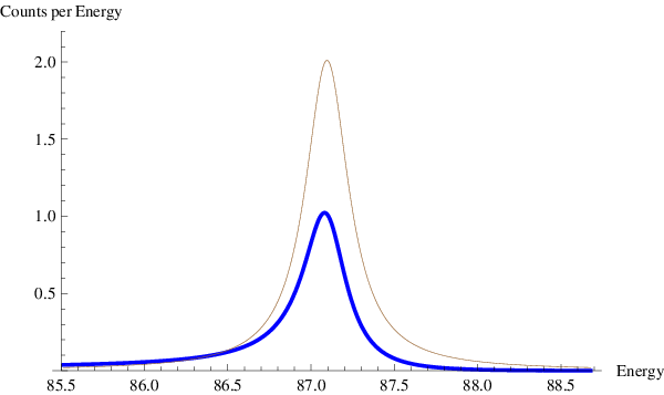
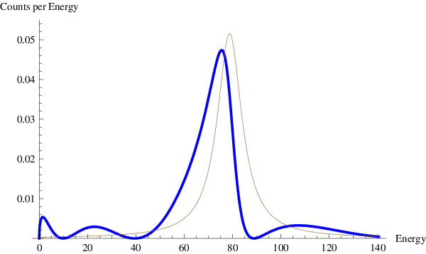
In Fig. 1 of Appendix C, we plot the decay energy spectrum of Eq. (5.5) along with the (normalized) Breit-Wigner distribution $\frac{1}{\pi}\frac{\Gamma_{\text{\tiny R}}/2}{(E-E_{\text{\tiny R}})^{2}+(\Gamma_{\text{\tiny R}}/2)^{2}}$ and the matrix element of the interaction $|\langle E|V|z_{\text{\tiny R}}\rangle|^{2}$ for the third resonance of the delta-shell potential when $\lambda=100$. For the sake of clarity, Fig. 2 of Appendix C contains the same plots as Fig. 1 except for the matrix element. Figure 3 displays the decay energy spectrum and the Breit-Wigner distribution of the third resonance when $\lambda=10$.

Figures 1-3 exhibit some features that are common to all the resonances produced by the delta-shell potential. First, although the lineshape of the resonant cross section (5.3) is given by the Lorentzian, the lineshape of the decay energy spectrum is not just the Breit-Wigner (Lorentzian) distribution. Rather, it is the Breit-Wigner distribution modulated by the matrix element. Second, the third resonance of the delta-shell potential is very sharp when $\lambda=100$, and in this case the decay energy spectrum is fairly symmetric and has a shape that is similar to the Breit-Wigner distribution (see Figs. 1 and 2). However, when $\lambda=10$, the third resonance is less sharp and the peak is more asymmetric (see Fig. 3). Although most experimental resonant peaks are symmetric, one can also find asymmetric ones, see for example figure 1 in Ref. [75] and figure 2b in Ref. [76]. In addition, when the resonance is very sharp, the tails of the decay energy spectrum tend smoothly to zero in regions away from the resonance’s position (see Figs. 1 and 2), whereas the tails of a resonance that is not so sharp have small wiggles (see Fig. 3). It is actually not unusual that decay spectra exhibit small wiggles, as can be seen for example in figure 1 of Ref. [77], figure 1b of Ref. [78], figure 1 of Ref. [79], and figure 2 of Ref. [80], although the wiggles of the figures of Refs. [77, 78, 79, 80] may be just statistical fluctuations. Third, fits using only the Breit-Wigner distribution would yield different resonant parameters than fits using the exact lineshape of Eq. (5.5). Fourth, it is clear from Fig. 1 that the matrix element is very different from either the Breit-Wigner distribution or from the resonant lineshape. Thus, the matrix element should not be used as the resonant lineshape. Fifth, Eq. (5.4) takes threshold effects into account automatically. In fact, one can see in Fig. 3 that there is a small enhancement of the decay energy spectrum at the $E=0$ threshold. Sixth, many resonant bumps are fitted by way of a Breit-Wigner distribution with an energy-dependent width. The resonant lineshape of Eq. (5.4) has an energy dependence carried by the matrix element, and therefore it may provide a useful alternative to Breit-Wigner distributions with an energy-dependent width. Seventh, experimental resonant peaks rarely have a Lorentzian shape, partly due to detector resolution. Often, when the pole width of the resonance is very small compared to the detector resolution, the width of the experimental peak is dominated by detector resolution, and the data are fit with a Gaussian distribution; when the pole width is comparable to the detector resolution, the data are fit with a Breit-Wigner distribution (for the resonant lineshape) convoluted by a Gaussian distribution (for the detector resolution). In fact, only in Mössbauer-like experiments one obtains peaks with Lorentzian shape. Thus, it is unlikely that the resonant lineshape of Eq. (5.4) shows up directly in most experiments, unless one makes use of a Mössbauer-like effect. Eighth, the resonant states are exponentially-growing, non-normalizable states, although they can be normalized using Zeldovich’s regulator. Surprisingly, though, they yield in a natural way a probability distribution that is finite without the need of any regulator. Ninth, it follows from Eqs. (3.7), (3.8) and (5.4) that

$$\frac{{\rm d}P(E)}{{\rm d}E}=\frac{1}{\,\overline{\Gamma}\,}\frac{{\rm d}\overline{\Gamma}(E)}{{\rm d}E}\,.$$

(5.6)

Hence, one can also use the decay width to obtain the decay energy spectrum of a resonant state. Tenth, similar to a Fano lineshape, the decay energy spectrum is asymmetric (although such asymmetry is barely noticeable when the resonance is sharp). However, whereas a Fano resonance appears in the cross section due to the interference between a scattering resonance and a background, the asymmetry of the decay energy spectrum is an intrinsic property of the decay of a resonance into the continuum.

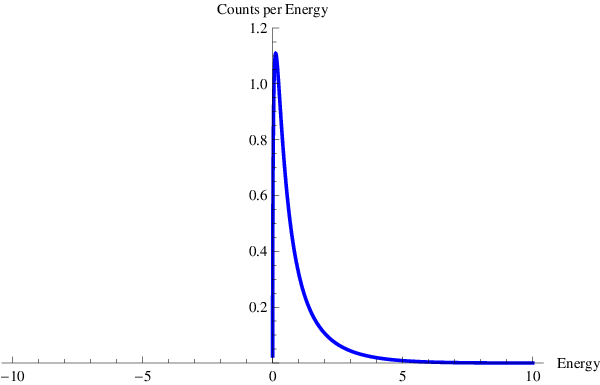
The decay energy spectra of the other resonances of the delta-shell potential are qualitatively the same as those shown in Figs. 1-3. However, for a virtual state, the decay energy spectrum has a different shape. Figure 4 shows the lineshape of the virtual state of the delta-shell potential when $\lambda=-0.5$. As can be seen in Fig. 4, the decay energy spectrum of a virtual state is simply a sharp peak located at the $E=0$ threshold. The peak has no resemblance with a Lorentzian. Rather, it is just a sharp enhancement of probability at the threshold, which is also how virtual states appear in cross sections.

In many systems, not just one but several resonances are excited. Figure 5 shows the decay energy spectrum of the first three resonances of the delta-shell potential when $\lambda=100$. Because each decay spectrum is normalized to 1, you can conclude from Fig. 5 that the peak of the first resonance is much sharper than the peak of the second resonance, which in turn is much sharper than the peak of the third resonance. This is a general feature: The higher the order of the resonance, the less sharp it is. In addition, as $|\lambda|$ decreases, the resonances become less sharp.

The natural question is, what kind of experiments would this resonant lineshape apply to? Let us imagine (for the sake of argument) that we have eight neutrons, six protons, and six electrons, and that we somehow have a procedure to produce a ¹⁴C atom out of them. Our experimental procedure would produce a state described by a square-integrable wave function $\varphi$. Assuming for simplicity that our system has only one resonance $z_{\text{\tiny R}}$, we can expand $\varphi$ as $\varphi=c_{\text{\tiny R}}|z_{\text{\tiny R}}\rangle+|\text{bg}\rangle$. When one devises an experimental procedure to produce a wave function very sharply tuned around the resonant state, the background term is nearly zero. However, $|\text{bg}\rangle$ can never be exactly zero, which reflects the experimental impossibility that a given preparation procedure always yields a resonant state. In the example of ¹⁴C atoms, this means that no matter what our procedure is to handle the protons, electrons and neutrons, we cannot always produce a ¹⁴C atom, not even in principle. During some trials, we will produce states that are not ¹⁴C atoms, and we identify such non-resonant states with the background. However, in those trials where we do produce a ¹⁴C atom, we let it decay. By repeating the process many times, and by discarding the trials where we do not produce a ¹⁴C atom, we measure the decay energy spectrum. Such spectrum should correspond to $\frac{{\rm d}P(E)}{{\rm d}E}$, because the wave function of the ¹⁴C atom would be a resonant state. Thus, in any experiment where we are able to create an unstable state that subsequently decays on its own, the decay energy spectrum would be given by $\frac{{\rm d}P(E)}{{\rm d}E}$.

There are many instances where two (or more) resonances interfere because they are not isolated from each other. The $S$-matrix description of such interference is as follows. Instead of the Laurent expansion of Eq. (5.2), one uses a Mittag-Leffler expansion. For our purposes, the Mittag-Leffler expansion can be easily obtained by means of Cauchy’s residue theorem, as done for example in Ref. [9]. Let us assume that $S(E)$ has two poles (a higher number of interfering resonances can be handled analogously) $z_{1}$ and $z_{2}$ in a region enclosed by a contour $\gamma$. The contour $\gamma$ also encloses a portion of the real axis, including the scattering energy $E$. Then Cauchy’s residue theorem implies that

$$\oint_{\gamma}\frac{S(w)-1}{w-E}{\rm d}w=2\pi{\rm i}\left(S(E)-1\right)+2\pi{\rm i}\left(\frac{{\rm r}_{1}}{z_{1}-E}+\frac{{\rm r}_{2}}{z_{2}-E}\right)\,,$$

(6.1)

where ${\rm r}_{1}$ and ${\rm r}_{2}$ are the residues of the $S$-matrix at $z_{1}$ and $z_{2}$, respectively. Equation (6.1) leads to the following Mittag-Leffler expansion:

$$S(E)-1=\left(\frac{{\rm r}_{1}}{E-z_{1}}+\frac{{\rm r}_{2}}{E-z_{2}}\right)+\frac{1}{2\pi{\rm i}}\oint_{\gamma}\frac{S(w)-1}{w-E}{\rm d}w\equiv\left(\frac{{\rm r}_{1}}{E-z_{1}}+\frac{{\rm r}_{2}}{E-z_{2}}\right)+B(E)\,,$$

(6.2)

where $B(E)$ is the background. By neglecting the background in the expansion (6.2), and by substituting the result into Eq. (5.1), we obtain that

$$\sigma(E)\approx\frac{\pi}{k^{2}}\left[\frac{|{\rm r}_{1}|^{2}}{(E-E_{1})^{2}+(\Gamma_{1}/2)^{2}}+\frac{|{\rm r}_{2}|^{2}}{(E-E_{2})^{2}+(\Gamma_{2}/2)^{2}}+2\,\text{Re}\left(\frac{{\rm r}_{1}{\rm r}_{2}^{*}}{(E-z_{1})(E-z_{2}^{*})}\right)\right].$$

(6.3)

Thus, the contribution to the cross section of two interference resonances consists of two Lorentzians (these are the contributions from each individual resonance) and an interference term.

When one measures the decay energy spectrum of two interfering resonances (see for example Ref. [81]), the quantity to consider is $\frac{{\rm d}P(E)}{{\rm d}E}$ rather than the cross section. As pointed out in Ref. [48], one can define the differential decay energy spectrum of any square-integrable function as

$$\frac{{\rm d}P(E)}{{\rm d}E}\equiv|\langle E|\varphi\rangle|^{2}\,.$$

(6.4)

When we describe a system of two interfering resonances, in analogy to Eq. (6.2), we expand $\varphi$ in terms of the corresponding resonant states as

$$|\varphi\rangle=c_{1}|z_{1}\rangle+c_{2}|z_{2}\rangle+|\text{bg}\rangle\,.$$

(6.5)

By neglecting the background $|\text{bg}\rangle$, we extract the contribution to $\varphi$ of those two resonances,

$$|\varphi\rangle\approx c_{1}|z_{1}\rangle+c_{2}|z_{2}\rangle\,.$$

(6.6)

By substituting Eq. (6.6) into Eq. (6.4), we obtain

$$\frac{{\rm d}P(E)}{{\rm d}E}=|c_{1}|^{2}|\langle E|z_{1}\rangle|^{2}+|c_{2}|^{2}|\langle E|z_{2}\rangle|^{2}+2\,\text{Re}(c_{1}c_{2}^{*}\langle E|z_{1}\rangle\langle E|z_{2}\rangle^{*})\,.$$

(6.7)

It was shown in section 3 of Ref. [48] that

$$\langle E|z_{1}\rangle=\frac{1}{z_{1}-E}\langle E|V|z_{1}\rangle\,,$$

(6.8)

with an analogous result holding for $|z_{2}\rangle$. Substitution of Eq. (6.8) into Eq. (6.7) yields

	$\displaystyle\frac{{\rm d}P(E)}{{\rm d}E}$	$\displaystyle=$	$\displaystyle|c_{1}|^{2}\frac{1}{(E-E_{1})^{2}+(\Gamma_{1}/2)^{2}}|\langle E|V|z_{1}\rangle|^{2}+|c_{2}|^{2}\frac{1}{(E-E_{2})^{2}+(\Gamma_{2}/2)^{2}}|\langle E|V|z_{2}\rangle|^{2}$		(6.9)
			$\displaystyle+2\,\text{Re}\left(c_{1}c_{2}^{*}\frac{1}{z_{1}-E}\frac{1}{z_{2}^{*}-E}\langle E|V|z_{1}\rangle\langle E|V|z_{2}\rangle^{*}\right)\,.$

This is the analog of Eq. (6.3). Both Eqs. (6.3) and (6.9) contain the contribution of each resonance plus an interference term. However, in Eq. (6.3) the contribution from each resonance to the cross section is fixed and determined by the Breit-Wigner distributions and the residues, whereas in Eq. (6.9) the contribution from each resonance can change depending on its weight ($c_{1}$ or $c_{2}$) in the resonant expansion (6.6).

It should be noted that the standard Golden Rule is unable to account for the interference of two resonances. The reason is that the interference between two delta functions should be zero, since there is no overlap between them. Thus, the standard Golden Rule does not produce an interference term, and it is inadequate to describe experiments such as, for example, that in Ref. [81].

In the literature, one can find studies of the interference of two resonances (see for example Refs. [24, 82, 83, 36]). The approach of the present paper is basically the same as that in Ref. [36]: One uses a resonant expansion [26, 28, 29, 30, 38, 43, 50] to expand a square integrable wave function in terms of resonant states, and then one keeps the contributions of the resonant states that carry the most weight in the expansion. It is important to understand, however, that resonant expansions [26, 28, 29, 30, 38, 43, 50] cannot be used to further expand the decay width, Eq. (3.3), the decay constant, Eq. (3.6), and the decay energy spectrum, Eq. (5.4), of a single resonance. The formulas in Eqs. (3.4), (3.6) and (5.4) already provide the contribution of each individual resonance, and therefore cannot be expanded any further in terms of the rest of the resonances of the system.

Fits of resonant peaks in cross sections are notoriously ambiguous, and one needs to recourse to additional quantities such as the phase shift or the time delay to ascertain the presence and the exact location of a resonance (see for example Ref. [84]). When a system has an isolated resonance, it is usually assumed [1] that in the vicinity of the resonant energy the $S$-matrix can be approximated by

$$S(E)\approx\frac{E-z_{\text{\tiny R}}^{*}}{E-z_{\text{\tiny R}}}\,.$$

(7.1)

Often, this approximation is written in terms of the wave number,

$$S(E)\approx\frac{k-k_{\text{\tiny R}}^{*}}{k-k_{\text{\tiny R}}}\,.$$

(7.2)

Mathematically, the approximations (7.1) and (7.2) can be justified by way of Blaschke products. Physically, such approximations are more desirable than the one resulting from neglecting the background in the Laurent expansion of the $S$-matrix, because the approximate $S$-matrix in Eqs. (7.1) and (7.2) is unitary, whereas the $S$-matrix that results from neglecting the background in the Laurent expansion is not unitary.

Because they are unitary, one may wonder if the approximations (7.1) and (7.2) lead to better fits of resonant peaks than the Laurent-expansion approximation. In order to find out, let us substitute Eq. (7.1) into Eq. (5.1). The result is

$$\sigma(E)\approx\sigma_{\text{\tiny e-unitarized}}(E)=\frac{\pi}{k^{2}}\frac{|\Gamma_{\text{\tiny R}}|^{2}}{(E-E_{\text{\tiny R}})^{2}+(\Gamma_{\text{\tiny R}}/2)^{2}}\,.$$

(7.3)

Similarly, substitution of Eq. (7.2) into Eq. (5.1) yields

$$\sigma(E)\approx\sigma_{\text{\tiny k-unitarized}}(E)=\frac{\pi}{k^{2}}\frac{|2\beta_{\text{\tiny R}}|^{2}}{(k-\alpha_{\text{\tiny R}})^{2}+\beta_{\text{\tiny R}}^{2}}\,.$$

(7.4)

Comparison of Eqs. (5.3), (7.3), and (7.4) shows that $\sigma_{\text{\tiny Laurent}}(E)$ and $\sigma_{\text{\tiny e-unitarized}}(E)$ are identical, except for an overall factor, whereas $\sigma_{\text{\tiny k-unitarized}}(E)$ is a Breit-Wigner distribution in the wave number [85], rather than in the energy, domain.

Figure 6 shows the three approximations together with the exact cross section in the vicinity of the third resonant energy for $\lambda=100$. As can be seen in Fig. 6, the approximations $\sigma_{\text{\tiny e-unitarized}}(E)$ and $\sigma_{\text{\tiny k-unitarized}}(E)$ are almost indistinguishable. In fact, their ratio is given by

$$\frac{\sigma_{\text{\tiny e-unitarized}}(E)}{\sigma_{\text{\tiny k-unitarized}}(E)}=\frac{4\alpha_{\text{\tiny R}}^{2}}{(k+\alpha_{\text{\tiny R}})^{2}+\beta_{\text{\tiny R}}^{2}}\,,$$

(7.5)

which is very close to unity when $k$ is close to $\alpha_{\text{\tiny R}}$ and when $\beta_{\text{\tiny R}}$ is small, as is the case for most resonances of the delta-shell potential when $|\lambda|$ is sufficiently large. One can also see in Fig. 6 that the Laurent approximation $\sigma_{\text{\tiny Laurent}}(E)$ is very similar to $\sigma_{\text{\tiny e-unitarized}}(E)$ and $\sigma_{\text{\tiny k-unitarized}}(E)$. Thus, even though the corresponding approximation of the $S$-matrix is not unitary, $\sigma_{\text{\tiny Laurent}}(E)$ provides as good of a fit as $\sigma_{\text{\tiny e-unitarized}}(E)$ and $\sigma_{\text{\tiny k-unitarized}}(E)$.

The resonant (Gamow) states are the natural wave functions of resonances. Because they diverge exponentially at infinity, it is not easy to extract information from them. We have used the delta-shell potential to show how one can calculate explicitly the decay width $\overline{\Gamma}$ and the decay constant $\Gamma$ of a resonant state without having to worry about its exponential blowup at infinity. We have also shown that the Golden Rule of a sharp resonant state yields a decay width that is approximately the same as the pole width, even though the exact decay width is very different from the pole width. Overall, the results of the present paper constitute a numerical validation of the formalism of Ref. [48].

It should be noted that the decay width $\overline{\Gamma}$ and the decay constant $\Gamma$ are not replacements of the pole width $\Gamma_{\text{\tiny R}}$, since $\Gamma_{\text{\tiny R}}$ determines the lifetime of the resonance. Rather, $\overline{\Gamma}$ and $\Gamma$ provide another way to quantify the strength of the interaction between the resonance and the continuum.

We have seen that for sharp resonances, the decay energy spectrum $\frac{{\rm d}P(E)}{{\rm d}E}$ has a shape that is similar to, but not the same as, the Breit-Wigner distribution, whereas for resonances that are not very sharp, the lineshape differs significantly from the Breit-Wigner distribution, due to the effect of the matrix element of the interaction. In particular, fits using the lineshape $\frac{{\rm d}P(E)}{{\rm d}E}$ would yield different resonant energies and pole widths than fits using only a Breit-Wigner distribution. We have also pointed out some (vague) similarities between the decay energy spectrum of the resonances of the delta-shell potential and some experimental decay energy spectra.

In normalizing the distribution $\frac{{\rm d}P(E)}{{\rm d}E}$, we have found that if we normalize a resonant state as $\frac{1}{\sqrt{\Gamma}}|z_{\text{\tiny R}}\rangle$, then $\frac{1}{\sqrt{\Gamma}}|z_{\text{\tiny R}}\rangle$ yields a normalized decay energy spectrum. However, this normalization is not a replacement of Zeldovich’s normalization, since Zeldovich’s normalization is more appropriate for resonant expansions.

We have seen that there is a clear analogy between the $S$-matrix description of a resonance and the formalism of Ref. [48]. Much like the pole of the $S$-matrix extracts the contribution of a resonance to the cross section through a Laurent expansion, the resonant state extracts the contribution of a resonance to the decay energy spectrum through the expression for $\frac{{\rm d}P(E)}{{\rm d}E}$. Much like Lorentzian peaks in the cross section are produced by intermediate, unstable particles, the quasi-Lorentzian peaks in decay energy spectra are produced by decaying, unstable particles.

There are however some differences between cross sections and decay energy spectra. For example, in the cross section, the contribution of each resonance is fixed, and it is determined by the residue of the $S$-matrix at the pole. In the decay energy spectrum the strength of each resonance’s contribution can change depending on the weight of that particular resonant state in the resonant expansion.

We have interpreted the background term of resonant expansions as the impossibility that a given experimental procedure used to create a resonant state is always successful. That is, not even in principle a given experimental procedure will yield a resonant state in all the trials. During some trials, a non-resonant state will be created, and such non-resonant state will be described by the background. However, in those trials where we do create a resonant state, the wave function of such state is a Gamow state, and the corresponding decay widths, decay constants, and decay energy spectra are obtained in the way presented in this paper.

We have argued that the standard Golden Rule is not appropriate to describe the interference of two resonances, and we have used the decay energy spectrum of two resonant states to describe such interference. The resulting energy spectrum is very similar to the cross section obtained by way of a Mittag-Leffler expansion.

We have also seen that three common approximations of the $S$-matrix lead to similar fits of resonant peaks in the cross section.

Although strictly speaking our results are restricted to the resonances of the delta-shell potential, it is likely that their main features hold true for a large class of potentials that includes those of compact support. However, it would be interesting to see how our results apply to more realistic systems [33, 86, 87, 88, 89, 90].

The author would like to thank Enriqueta Hernandez, Martin Tchernookov, Cengiz Sen, and George Irwin for enlightening discussions.

References

- [1] J.R. Taylor, Scattering Theory, John Wiley & Sons (1972).
- [2] A. Sirlin, Phys. Rev. Lett. 67, 2127 (1991).
- [3] S. Willenbrock and G. Valencia, Phys. Lett. B 259, 373 (1991).
- [4] R.G. Stuart, Phys. Lett. B 262, 113 (1991).
- [5] A. Leike, T. Riemann, and J. Rose, Phys. Lett. B 273, 513 (1991).
- [6] A. Bernicha, G. Lopez Castro, and J. Pestieau, Phys. Rev. D 50, 4454 (1994); Nucl. Phys. A 597, 623 (1996).
- [7] Particle Data Group, S. Eidelman et al., Phys. Lett. B 592, 1 (2004).
- [8] A.R. Bohm, Y. Sato, Phys. Rev. D 71, 085018 (2005).
- [9] S.A. Rakityansky, N. Elander, Int. J. Quant. Chemistry 106 1105 (2006); arXiv:1110.4990.
- [10] D. Djukanovic, J. Gegelia, S. Scherer, Phys. Rev. D 76, 037501 (2007); arXiv:0707.2030
- [11] S.A. Rakityansky, S.A. Sofianos, N. Elander, J. Phys. A: Math. Theor. 40, 14857 (2007); arXiv:1110.4988.
- [12] K. Shilyaeva, E. Yarevsky, N. Elander, J. Phys. B: Atom. Mol. Opt. Phys. 42, 044011 (2009).
- [13] M. Hadžimehmedović, S. Ceci, A. Švarc, H. Osmanović, J. Stahov, Phys. Rev. C 84, 035204 (2011); arXiv:1103.2653.
- [14] S. Ceci, M. Korolija, B. Zauner, Phys. Rev. Lett. 111, 112004 (2013); arXiv:1302.3491.
- [15] R.L. Workman, L. Tiator, A. Sarantsev Phys.Rev. C 87, 068201 (2013); arXiv:1304.4029.
- [16] K.A. Olive et al. (Particle Data Group), Chin. Phys. C 38, 090001 (2014).
- [17] A. Švarc, M. Hadžimehmedović, H. Osmanović, J. Stahov, L. Tiator, R.L. Workman, Phys. Rev. C 89, 065208 (2014); arXiv:1404.1544.
- [18] P. Vaandrager, S.A. Rakityansky, Int. J. Mod. Phys. E, 25, 1650014 (2016); arXiv:1603.01718.
- [19] L. Tiator, M. Döring, R.L. Workman, M. Hadžimehmedović, H. Osmanović, R. Omerović, J. Stahov, A. Švarc, Phys. Rev. C 94, 065204 (2016); arXiv:1606.00371.
- [20] G. Gamow, Z. Phys. 51, 204 (1928).
- [21] A.F.J. Siegert, Phys. Rev. 56, 750 (1939).
- [22] Ya.B. Zeldovich, Sov. Phys. JETP 12, 542 (1961).
- [23] T. Berggren, Nucl. Phys. A 109, 265 (1968).
- [24] U. Peskin, H. Reisler, W.H. Miller, J. Chem. Phys. 101, 9672 (1994).
- [25] C.G. Bollini, O. Civitarese, A.L. De Paoli, M.C. Rocca, Phys. Lett. B382, 205 (1996).
- [26] O.I. Tolstikhin, V.N. Ostrovsky, H. Nakamura, Phys. Rev. A 58, 2077 (1998).
- [27] E. Hernández, A. Jáuregui, A. Mondragón, J. Phys. A: Math. Gen. 33, 4507 (2000).
- [28] R. de la Madrid, G. Garcia-Calderon, J.G. Muga, Czech. J. Phys. 55, 1141 (2005); quant-ph/0512242.
- [29] O.I. Tolstikhin, Phys. Rev. A 73, 062705 (2006).
- [30] O.I. Tolstikhin, Phys. Rev. A 77, 032712 (2008).
- [31] J.M. Velazquez-Arcos, C.A. Vargas, J.L. Fernandez-Chapou, A.L. Salas-Brito, J. Math. Phys. 49, 103508 (2008).
- [32] R. de la Madrid, Nucl. Phys. A 812, 13 (2008); arXiv:0810.0876.
- [33] N. Michel, W. Nazarewicz, M. Ploszajczak, T. Vertse, J. Phys. G: Nucl. Part. Phys. 36, 013101 (2009); arXiv:0810.2728.
- [34] T. Goldzak, I. Gilary, N. Moiseyev, Phys. Rev. A 82, 052105 (2010).
- [35] G. Garcia-Calderon, Advances in Quantum Chemistry 60, 407 (2010).
- [36] K. Sasada, N. Hatano, G. Ordonez, J. Phys. Soc. Jpn. 80, 104707 (2011); arXiv:0905.3953.
- [37] G. Garcia-Calderon, L.G. Mendoza-Luna, Phys. Rev. A 84, 032106 (2011); arXiv:1104.4688.
- [38] G. Garcia-Calderon, A. Mattar, J. Villavicencio, Phys. Scr. T151, 01476 (2012); arXiv:1205.0487.
- [39] L. Chaos-Cador, G. Garcia-Calderon, Phys. Rev. A, 87, 042114 (2013).
- [40] K. Fossez, N. Michel, W. Nazarewicz, M. Płoszajczak, Phys. Rev. A, 87, 042515 (2013); arXiv:1303.1928.
- [41] C.K. Andersen, K. Mølmer, Phys. Rev. A 87, 052119 (2013); arXiv:1303.5644.
- [42] J. Julve, S. Turrini, F.J. de Urríes, Int. J. Theo. Phys. 53, 971 (2014); arXiv:1302.0630.
- [43] N. Hatano, G. Ordonez, J. Math. Phys. 55 122106 (2014); arXiv:1405.6683.
- [44] G. Garcia-Calderon, L. Chaos-Cador, Phys. Rev. A 90, 032109 (2014); arXiv:1605.00999
- [45] S. Cruz y Cruz, O. Rosas-Ortiz, Adv. Math. Phys. 281472 (2015); arXiv:1504.01008.
- [46] R. Lundmark, C. Forssén, J. Rotureau, Phys. Rev. A, 91, 041601 (2015); arXiv:1412.7175.
- [47] S. Gentilini, M.C. Braidotti, G. Marcucci, E. DelRe, C. Conti, Phys. Rev. A, 92, 023801 (2015); arXiv:1508.00692.
- [48] R. de la Madrid, Nucl. Phys. A 940, 297 (2015); arXiv:1505.07139.
- [49] G. Garcia-Calderon, R. Romo, Phys. Rev A, 93, 022118 (2016).
- [50] J.M. Brown, P. Jakobsen, A. Bahl, J.V. Moloney, M. Kolesik, J. Math. Phys. 57, 032105 (2016).
- [51] A. Plastino, M.C. Rocca, Nucl. Phys. A, 948, 19 (2016); arXiv:1511.04010.
- [52] A. Plastino, M.C. Rocca, D.J. Zamora Nucl. Phys. A, 955, 16 (2016); arXiv:1604.06910.
- [53] D. Cevik, M. Gadella, S. Kuru, J. Negro, Phys. Lett. A 380, 1600 (2016); arXiv:1601.05134.
- [54] O. Olendski, Ann. Phys. (Berlin), 529 1600144 (2017); arXiv:1611.00197.
- [55] S. Garmon, G. Ordonez, arXiv:1609.07718.
- [56] G. Garcia-Calderon, L. Chaos-Cador, Fortschritte der Physik (to be published); arXiv:1702.02247.
- [57] D. Carlsmith, Particle Physics, Pearson (2012).
- [58] R.G. Winter, Phys. Rev. 123, 1503 (1961).
- [59] K. Gottfried, Quantum Mechanics, W.A. Benjamin (1966).
- [60] D.A. Dicus, W.W. Repko, R.F. Schwitters, T.M. Tinsley, Phys. Rev. A 65, 032116 (2002).
- [61] T.C. Scott, J.F. Babb, A. Dalgarno, J.D. Morgan III, J. Chem. Phys. 99 2841 (1993).
- [62] U.G. Aglietti, P.M. Santini, Phys. Rev. A 89, 022111 (2014); arXiv:1303.4977.
- [63] U.G. Aglietti, P.M. Santini, J. Math. Phys. 56, 062104 (2015); arXiv:1503.02532.
- [64] E. Segrè, Nuclei and Particles: An Introduction to Nuclear and Subnuclear Physics, Benjamin-Cummings Publishing Company, 2nd edition (1977).
- [65] J.H. Lambert, Acta Helveticae physico-mathematico-anatomico-botanico-medica, Band III, 128 (1758).
- [66] L. Euler, Acta Acad. Scient. Petropol. 2, 29 (1783).
- [67] R.M. Corless, G.H. Gonnet, D.E.G. Hare, D.J. Jeffrey, D.E. Knuth, Advances in Computational Mathematics 5, 329 (1996).
- [68] https://en.wikipedia.org/wiki/Lambert-W-function.
- [69] http://mathworld.wolfram.com/LambertW-Function.html
- [70] A.M. Ishkhanyan, Phys. Lett. A 380, 640 (2016); arXiv:1509.00846.
- [71] Since the Lambert function has rarely been used in the physics literature, we devote Appendix A to show that the solutions of Eq. (2.5) can indeed be written in terms of .
- [72] A. Andreassen, D. Farhi, W. Frost, M.D. Schwartz, Phys. Rev. Lett. 117, 231601 (2016); arXiv:1602.01102.
- [73] A. Andreassen, D. Farhi, W. Frost, M.D. Schwartz, arXiv:1604.06090.
- [74] Essentially, these are also the conditions under which the resonant amplitude of a Gamow state can be identified with the Breit-Wigner amplitude [32].
- [75] BESIII Collaboration, arXiv:1612.05721.
- [76] F. Dettori (for the LHCb Collaboration), arXiv:1611.06717.
- [77] LHCb Collaboration, JHEP 03 (2016) 040 arXiv:1601.05284.
- [78] LHCb Collaboration, Phys. Lett. B 757, 558 (2016); arXiv:1510.08367.
- [79] LHCb Collaboration, Eur. Phys. J. C, 77, 72 (2017); arXiv:1610.01383.
- [80] LHCb Collaboration, Phys. Rev. D 95, 012006 (2017); arXiv:1610.05187.
- [81] BESIII Collaboration, Phys. Rev. Lett. 117, 042002 (2016); arXiv:1603.09653.
- [82] A.I. Magunov, I. Rotter, and S.I. Strakhova, Phys. Rev. B 68, 245305 (2003); arXiv:quant-ph/0305064.
- [83] I. Rotter, arXiv:0711.2926.
- [84] G.A. Luna-Acosta, A.A. Fernández-Marín, J. A. Méndez-Bermúdez, C. Poli, Phys. Lett. A 380, 2494 (2016); arXiv:1606.00326.
- [85] For a q-extension of momentum Breit-Wigner distributions, see Refs. [51, 52].
- [86] H. Kamano, S.X. Nakamura, T.-S.H. Lee, T. Sato, Phys. Rev. C 92, 025205 (2015); arXiv:1506.01768.
- [87] K. Miyahara, T. Hyodo, Phys. Rev. C 93, 015201 (2016); arXiv:1506.05724.
- [88] H. Kamano, S.X. Nakamura, T.-S.H. Lee, T. Sato, Phys. Rev. C 94, 015201 (2016); arXiv:1605.00363.
- [89] H. Kamano, T.-S.H. Lee, Phys. Rev. C 94, 065205 (2016); arXiv:1608.03470.
- [90] A. Flores-Tlalpa, G. López Castro, P. Roig, J. High Energy Phys. 04, 185 (2016); arXiv:1508.01822.