跳到论文正文
W Papers独立论文阅读器 arXiv:1704.00030 论文正文 计算阅读时间 · 0%
引用这篇论文根据当前论文元数据生成,正式投稿前建议核对。


License: arXiv.org perpetual non-exclusive license
arXiv:1704.00030v2 [math-ph] 02 Oct 2017

Orbits in the problem of two fixed centers on the sphere

M.A. Gonzalez Leon Note: E-mail: magleon@usal.es Affiliation: Departamento de Matemática Aplicada, University of SalamancaAvd. Filiberto Villalobos 119, 37007 Salamanca, Spain    J. Mateos Guilarte Note: E-mail: guilarte@usal.es Affiliation: Departamento de Física Fundamental, University of SalamancaFacultad de Ciencias, Casas del Parque II, 37008 Salamanca, Spain    M. de la Torre Mayado Note: E-mail: marina@usal.es Affiliation: Departamento de Física Fundamental, University of SalamancaFacultad de Ciencias, Casas del Parque II, 37008 Salamanca, Spain
Abstract

A trajectory isomorphism between the two Newtonian fixed center problem in the sphere and two associated planar two fixed center problems is constructed by performing two simultaneous gnomonic projections in S2S^{2}. This isomorphism converts the original quadratures into elliptic integrals and allows the bifurcation diagram of the spherical problem to be analyzed in terms of the corresponding ones of the planar systems. The dynamics along the orbits in the different regimes for the problem in S2S^{2} is expressed in terms of Jacobi elliptic functions.

MSC2010 numbers: 70F15, 70H06.

Keywords: spherical two-center problem, separation of variables, spheroconical coordinates, elliptic coordinates.

1 Introduction

The two fixed center problem on the two-dimensional sphere goes back to Killing [21], and in modern times to Kozlov and Harin [22], who proved the separability of the problem, thus its integrability, in sphero-conical coordinates. These coordinates on S2S^{2} were introduced by Liouville [25], and independently by Neumann [27] in one of the first examples of dynamics in spaces of constant curvature, and they are closely related to elliptic coordinates, in fact, the first system of coordinates plays a role in the dynamics on the sphere completely similar to the second system with respect to the Euclidian case. Integrability and Hamilton-Jacobi separability in sphero-conical coordinates has been constructed for different physical systems defined on the sphere, see, for instance, [11]. In particular, the authors analyzed in this context the Neumann problem and the Garnier system on S2S^{2} in order to study solitary waves in one-dimensional nonlinear S2S^{2}-sigma models, see [7] and [8]. A detailed historical review of several systems defined in spaces of constant curvature, including open problems, has been recently performed in [14], where a precise bibliography is contained.

The two fixed center problem on the sphere is the superposition of two Kepler problems on S2S^{2}. An explicit expression for the second constant of motion for this problem and also for some generalizations was given in [26, 12]. In [13] Borisov and Mamaev, inspired by a previous work of Albouy and Stuchi [1, 2], established a trajectory isomorphism between the orbits lying in the half-sphere that contains the two attractive centers and the bounded orbits of an associated planar system of two attractive centers.

This isomorphism is constructed using a gnomonic projection from S2S^{2} to the tangent plane at the middle point between the centers. The idea of relating planar and spherical problems in the framework of general force fields by considering the gnomonic projection goes back to Appell [9, 10], who also explained in this context the previous results of Serret [30] about the one fixed center problem on the sphere. Almost one century later Higgs [19] rediscovered these techniques. More recently, Albouy has developed these ideas and extended their scope to a general projective dynamics [1, 2, 3, 4, 5].

In this work we extend the results of [13] to the whole sphere, i.e., we establish a trajectory isomorphism between the complete set of orbits of the original problem and the corresponding one to two associated planar problems. The underlying idea is to identify each trajectory crossing the equator with the conjunction of two planar unbounded orbits, one of the two attractive center problem and another one for the system of two repulsive centers.

The extended trajectory isomorphism allows us to understand the bifurcation diagram of the spherical problem, previously analyzed in [31, 32, 33], as the superposition of the diagrams corresponding to the planar problem of two attractive centers [34] plus those associated to two repulsive centers [29]. This point of view permits the identification of the domains of allowable motions and the different cases for orbits, already described in [33], in terms of their partners for the planar diagrams. Finally, these identifications lead in a natural way to the determination of the quadratures (elliptic integrals) for the parametric equations of the orbits in terms of a local time. Using adequately the properties of elliptic integrals, the quadratures are inverted to obtain explicit formulas in terms of Jacobi elliptic functions for the different types of orbits of the spherical problem.

The existence of closed orbits in the sphere is guaranteed for the case of commensurability between the involved periods of the Jacobi functions.

The structure of the paper is as follows: The problem is presented in Section 2 using sphero-conical coordinates on S2S^{2}. In Section 3 the extended trajectory isomorphism is defined, and thus the quadratures are converted into elliptic integrals. The bifurcation diagram for the spherical problem is constructed from the diagrams of the two associated planar problems in Section 4. Finally, in Section 5, the process of inversion of elliptic integrals in S2S^{2} is detailed, and general expressions for the solutions are shown.

The complete list of analytical expressions for the different types of orbits in S2S^{2}, in terms of a local time, is included in the Appendix, together with a gallery of figures for all the significative cases.

2 The two Newtonian centers problem in S2S^{2}

We consider the problem of a unit mass lying on the sphere S2S^{2} of radius RR, viewed as immersed in the Euclidean space ℝ3{\mathbb{R}}^{3} with Cartesian coordinates (X,Y,Z)(X,Y,Z):

X2+Y2+Z2=R2X^{2}+Y^{2}+Z^{2}=R^{2}

under the influence of the superposition of two Kepler potentials on S2S^{2}, i.e., the potential:

𝒰(θ1,θ2)=−γ1Rcotanθ1−γ2Rcotanθ2,{\cal U}(\theta_{1},\theta_{2})\,=\,-\frac{\gamma_{1}}{R}\mathop{\rm cotan}\nolimits\theta_{1}-\frac{\gamma_{2}}{R}\mathop{\rm cotan}\nolimits\theta_{2}, (1)

Refer to caption

Figure 1: Location of the two Newtonian centers F1F_{1} and F2F_{2} in S2S^{2}. The angular separation is 2​θf2\theta_{f}, with 0<θf<π20<\theta_{f}<\frac{\pi}{2}. θ1\theta_{1} and θ2\theta_{2} denote the great circle angles between a given point P∈S2P\in S^{2} and F1F_{1} and F2F_{2}, respectively.

where θ1\theta_{1} and θ2\theta_{2} denote the great circle angles between the location of the centers F1F_{1} and F2F_{2}, see Fig. 1, and a given point PP on S2S^{2}, in such a way that R​θ1R\theta_{1} and R​θ2R\theta_{2} are the orthodromic distances from F1F_{1} and F2F_{2} to PP, respectively. γ1\gamma_{1} and γ2\gamma_{2} are the strengths of the centers, where we have considered 0<γ2≤γ10<\gamma_{2}\leq\gamma_{1}, i.e., the test mass feels the presence of two attractive centers in F1F_{1} and F2F_{2}, and correspondingly two repulsive centers at their antipodal points F¯1\bar{F}_{1} and F¯2\bar{F}_{2}. Without loss of generality, the chosen points, notation and orientation are shown in Fig. 1. Thus, the Cartesian coordinates of F1F_{1} and F2F_{2} are (Rsinθf,0,Rcosθf)=(Rσ¯,0,Rσ)(R\sin\theta_{f},0,R\cos\theta_{f})=(R\bar{\sigma},0,R\sigma) and (−Rsinθf,0,Rcosθf)=(−Rσ¯,0,Rσ)(-R\sin\theta_{f},0,R\cos\theta_{f})=(-R\bar{\sigma},0,R\sigma), respectively. Parameters σ=cos⁡θf\sigma=\cos\theta_{f} and σ¯=sin⁡θf\bar{\sigma}=\sin\theta_{f} have been introduced in order to alleviate the notation.

This problem is completely integrable, see, e.g., [21, 22], there exist two constants of motion, the Hamiltonian:

ℋ=12​R2​(LX2+LY2+LZ2)−1R​(γ1​(σ​Z+σ¯​X)R2−(σ​Z+σ¯​X)2+γ2​(σ​Z−σ¯​X)R2−(σ​Z−σ¯​X)2),{\cal H}=\frac{1}{2R^{2}}\left(L_{X}^{2}+L_{Y}^{2}+L_{Z}^{2}\right)-\frac{1}{R}\left(\frac{\gamma_{1}(\sigma\,Z+\bar{\sigma}\,X)}{\sqrt{R^{2}-(\sigma\,Z+\bar{\sigma}\,X)^{2}}}+\frac{\gamma_{2}(\sigma\,Z-\bar{\sigma}\,X)}{\sqrt{R^{2}-(\sigma\,Z-\bar{\sigma}\,X)^{2}}}\right), (2)

where L→=X→×P→\vec{L}=\vec{X}\times\vec{P}, P→=(PX,PY,PZ),X→=(X,Y,Z)\vec{P}=(P_{X},P_{Y},P_{Z}),\vec{X}=(X,Y,Z), and the second invariant:

Ω=12​R2​(LX2+σ2​LY2)−σR​(γ1​ZR2−(σ​Z+σ¯​X)2+γ2​ZR2−(σ​Z−σ¯​X)2).\Omega=\frac{1}{2R^{2}}\left(L_{X}^{2}+\sigma^{2}L_{Y}^{2}\right)-\frac{\sigma}{R}\left(\frac{\gamma_{1}\,Z}{\sqrt{R^{2}-(\sigma\,Z+\bar{\sigma}\,X)^{2}}}+\frac{\gamma_{2}\,Z}{\sqrt{R^{2}-(\sigma\,Z-\bar{\sigma}\,X)^{2}}}\right). (3)

This constant of motion is slightly different, but equivalent to the invariant obtained by Borisov and Mamaev in [26, 12]. Potential (1) can be rewritten as

𝒰⁡(θ1,θ2)=−(γ1+γ2)​sin⁡θ1+θ22​cos⁡θ1+θ22+(γ1−γ2)​sin⁡θ2−θ22​cos⁡θ2−θ12R⁡(sin2⁡θ1+θ22−sin2⁡θ2−θ12){\cal U}(\theta_{1},\theta_{2})=-\,\frac{(\gamma_{1}+\gamma_{2})\sin\frac{\theta_{1}+\theta_{2}}{2}\,\cos\frac{\theta_{1}+\theta_{2}}{2}+(\gamma_{1}-\gamma_{2})\sin\frac{\theta_{2}-\theta_{2}}{2}\,\cos\frac{\theta_{2}-\theta_{1}}{2}}{R\left(\sin^{2}\frac{\theta_{1}+\theta_{2}}{2}-\sin^{2}\frac{\theta_{2}-\theta_{1}}{2}\right)} (4)

in such a way that it is natural to introduce an á la Euler version of sphero-conical coordinates on S2S^{2}, i.e.,

U=sin⁡θ1+θ22,V=sin⁡θ2−θ12;−σ¯<V<σ¯,σ¯<U<1U=\sin\frac{\theta_{1}+\theta_{2}}{2}\ ,\quad V=\sin\frac{\theta_{2}-\theta_{1}}{2}\ ;\quad-\bar{\sigma}<V<\bar{\sigma}\ ,\quad\bar{\sigma}<U<1

Coordinate lines with fixed UU or VV resemble “spherical ellipses” or “spherical hyperbolas”, respectively, with foci F1F_{1} and F2F_{2}, with the understanding that “spherical hyperbolas” are nothing more than “spherical ellipses” with respect to the pair of foci F¯1\bar{F}_{1} and F2F_{2} or F1F_{1} and F¯2\bar{F}_{2}.

The change of coordinates

X=Rσ¯​U​V,Y2=R2σ2​σ¯2​(U2−σ¯2)​(σ¯2−V2),Z2=R2σ2​(1−U2)​(1−V2)X=\frac{R}{\bar{\sigma}}U\,V\ ,\quad Y^{2}=\frac{R^{2}}{\sigma^{2}\bar{\sigma}^{2}}(U^{2}-\bar{\sigma}^{2})\,(\bar{\sigma}^{2}-V^{2})\ ,\quad Z^{2}=\frac{R^{2}}{\sigma^{2}}(1-U^{2})\,(1-V^{2}) (5)

is a four-to-one map because of the ambiguities in the signs of YY and ZZ. Obviously, coordinates UU and VV are dimensionless.

Potential (4) is written in these sphero-conical coordinates with two different expressions depending on the hemisphere that it is considered. For S+2={(X,Y,Z)∈S2,Z≥0}S^{2}_{+}=\{(X,Y,Z)\in S^{2},\ Z\geq 0\}, we have

𝒰+​(U,V)=−1R⁡(U2−V2)​((γ1+γ2)​U​1−U2+(γ1−γ2)​V​1−V2),{\cal U}_{+}(U,V)=-\frac{1}{R(U^{2}-V^{2})}\left((\gamma_{1}+\gamma_{2})U\sqrt{1-U^{2}}+(\gamma_{1}-\gamma_{2})V\sqrt{1-V^{2}}\right), (6)

whereas in S−2={(X,Y,Z)∈S2,Z≤0}S^{2}_{-}=\{(X,Y,Z)\in S^{2},\ Z\leq 0\} the potential reads:

𝒰−​(U,V)=−1R⁡(U2−V2)​(−(γ1+γ2)​U​1−U2+(γ1−γ2)​V​1−V2).{\cal U}_{-}(U,V)=-\frac{1}{R(U^{2}-V^{2})}\left(-(\gamma_{1}+\gamma_{2})U\sqrt{1-U^{2}}+(\gamma_{1}-\gamma_{2})V\sqrt{1-V^{2}}\right). (7)

Note that both expressions (6) and (7) coincide on the Equator Z=0Z=0, or U=1U=1. Thus, Hamiltonian (2) has also to be split into two different expressions:

ℋ±=12​R2​(U2−V2)​((U2−σ¯2)​(1−U2)​pU2+(σ¯2−V2)​(1−V2)​pV2)+𝒰±​(U,V).{\cal H}_{\pm}=\frac{1}{2R^{2}(U^{2}-V^{2})}\left((U^{2}-\bar{\sigma}^{2})(1-U^{2})p_{U}^{2}+(\bar{\sigma}^{2}-V^{2})(1-V^{2})p_{V}^{2}\right)+{\cal U}_{\pm}(U,V). (8)

The Hamilton-Jacobi equations coming from (8)

ℋ±​(∂S∂U,∂S∂V,U,V)+∂S∂t=0{\cal H}_{\pm}\left(\frac{\partial S}{\partial U},\frac{\partial S}{\partial V},U,V\right)+\frac{\partial S}{\partial t}=0 (9)

are separable into two ordinary differential equations if we look for solutions of the form: S±​(t,U,V)=St​(t)+SU±​(U)+SV​(V)S_{\pm}(t;U,V)=S_{t}(t)+S_{U\pm}(U)+S_{V}(V). Introducing nondimensional variables

ℋ±→γ1+γ2R​ℋ±,t→R3γ1+γ2​t,pU,V→R⁡(γ1+γ2)​pU,V{\cal H}_{\pm}\to\frac{\gamma_{1}+\gamma_{2}}{R}{\cal H}_{\pm}\ ,\quad t\to\frac{\sqrt{R^{3}}}{\sqrt{\gamma_{1}+\gamma_{2}}}\,t\ ,\quad p_{U,V}\to\sqrt{R(\gamma_{1}+\gamma_{2})}p_{U,V}

and defining the parameter

γ=γ2γ1+γ2,\gamma=\frac{\gamma_{2}}{\gamma_{1}+\gamma_{2}},

the complete solution of (9) is

S±​(t,U,V)\displaystyle S_{\pm}(t;U,V) =\displaystyle= −H​t+sg⁡(pU)​2​∫σ¯UH​U2±U​1−U2−G(1−U2)​(U2−σ¯2)​𝑑U\displaystyle-Ht+{\rm sg}(p_{U})\sqrt{2}\int_{\bar{\sigma}}^{U}\frac{\sqrt{HU^{2}\pm U\sqrt{1-U^{2}}-G}}{\sqrt{(1-U^{2})(U^{2}-\bar{\sigma}^{2})}}dU
+sg(pV)2∫−σ¯V−H​V2+(1−2​γ)​V​1−V2+G(σ¯2−V2)​(1−V2)dV,\displaystyle+{\rm sg}(p_{V})\sqrt{2}\int_{-{\bar{\sigma}}}^{V}\frac{\sqrt{-HV^{2}+(1-2\gamma)V\sqrt{1-V^{2}}+G}}{\sqrt{(\bar{\sigma}^{2}-V^{2})(1-V^{2})}}dV,

where HH and GG are the values of the constants of motion: ℋ=H{\cal H}=H, 𝒢=G{\cal G}=G; 𝒢{\cal G} is the separation constant related to Ω\Omega and ℋ{\cal H}, (3) and (2), by the expression

𝒢=ℋ−Ω.{\cal G}\,={\cal H}-\Omega.

Given the local time ς\varsigma by d​ς=d​tU2−V2d\varsigma=\frac{dt}{U^{2}-V^{2}}, the standard separation procedure leads us to the first-order equations

d​Ud​ς\displaystyle\frac{dU}{d\varsigma} =\displaystyle= sg⁡(pU)​2​(1−U2)​(U2−σ¯2)​(H​U2+U​1−U2−G)\displaystyle{\rm sg}(p_{U})\,\sqrt{2}\,\sqrt{(1-U^{2})(U^{2}-\bar{\sigma}^{2})(HU^{2}+U\sqrt{1-U^{2}}-G)} (10)
d​Vd​ς\displaystyle\frac{dV}{d\varsigma} =\displaystyle= sg⁡(pV)​2​(1−V2)​(σ¯2−V2)​(−H​V2+(1−2​γ)​V​1−V2+G)\displaystyle{\rm sg}(p_{V})\,\sqrt{2}\,\sqrt{(1-V^{2})(\bar{\sigma}^{2}-V^{2})(-HV^{2}+(1-2\gamma)V\sqrt{1-V^{2}}+G)} (11)

for the problem in the Northern hemisphere S+2S_{+}^{2}, and

d​Ud​ς\displaystyle\frac{dU}{d\varsigma} =\displaystyle= sg⁡(pU)​2​(1−U2)​(U2−σ¯2)​(H​U2−U​1−U2−G)\displaystyle{\rm sg}(p_{U})\,\sqrt{2}\,\sqrt{(1-U^{2})(U^{2}-\bar{\sigma}^{2})(HU^{2}-U\sqrt{1-U^{2}}-G)} (12)
d​Vd​ς\displaystyle\frac{dV}{d\varsigma} =\displaystyle= sg⁡(pV)​2​(1−V2)​(σ¯2−V2)​(−H​V2+(1−2​γ)​V​1−V2+G)\displaystyle{\rm sg}(p_{V})\,\sqrt{2}\,\sqrt{(1-V^{2})(\bar{\sigma}^{2}-V^{2})(-HV^{2}+(1-2\gamma)V\sqrt{1-V^{2}}+G)} (13)

for the Southern S−2S_{-}^{2} one.

A direct attack to the quadratures involved looks apparently cumbersome and, as far as we know, they are not solved in the literature. Nevertheless, some of the qualitative and topological properties of these orbits have been analyzed in [31, 32, 33].

3 Trajectory isomorphism between the spherical and two different planar problems

Following Borisov & Mamaev [13], we go back to Cartesian coordinates (X,Y,Z)(X,Y,Z) where the potential (1) can be written as

𝒰⁡(X,Y,Z)=−1R​(γ1​(σ​Z+σ¯​X)R2−(σ​Z+σ¯​X)2+γ2​(σ​Z−σ¯​X)R2−(σ​Z−σ¯​X)2).{\cal U}(X,Y,Z)\,=\,-\frac{1}{R}\left(\frac{\gamma_{1}(\sigma\,Z+\bar{\sigma}\,X)}{\sqrt{R^{2}-(\sigma\,Z+\bar{\sigma}\,X)^{2}}}+\frac{\gamma_{2}(\sigma\,Z-\bar{\sigma}\,X)}{\sqrt{R^{2}-(\sigma\,Z-\bar{\sigma}\,X)^{2}}}\right). (14)

The corresponding Newton equations for this problem are

X¨=−∂𝒰∂X+λ​X,Y¨=−∂𝒰∂Y+λ​Y,Z¨=−∂𝒰∂Z+λ​Z,\ddot{X}\,=\,-\frac{\partial{\cal U}}{\partial X}\,+\,\lambda X\ ,\quad\ddot{Y}\,=\,-\frac{\partial{\cal U}}{\partial Y}\,+\,\lambda Y\ ,\quad\ddot{Z}=-\frac{\partial{\cal U}}{\partial Z}\,+\,\lambda Z, (15)

where the dots represent derivatives with respect to the physical (dimensional) time tt and λ\lambda is the Lagrange multiplier. In [13] it was proved that the gnomonic projection from S+2S_{+}^{2} to the tangent plane Π+\Pi_{+} at the point (0,0,R)(0,0,R), together with a linear transformation in Π+\Pi_{+}, maps Newton equations (15) to the Newton equations of an associated problem of two attractive centers in ℝ2{\mathbb{R}}^{2}.

Here, we shall also consider simultaneously another gnomonic projection, from S−2S_{-}^{2} to the tangent plane Π−\Pi_{-}, at (0,0,−R)(0,0,-R). The projected coordinates (x,y)(x,y) are given in the two planes by

Π+:x=RZX,y=RZY;Π−:x=R−ZX,y=R−ZY.\Pi_{+}:\quad x=\frac{R}{Z}\,X\ ,\quad y=\frac{R}{Z}\,Y\quad;\quad\Pi_{-}:\quad x=\frac{R}{-Z}\,X\ ,\quad y=\frac{R}{-Z}\,Y. (16)

for Z≠0Z\neq 0. The Equator is mapped to the infinity in both Π+\Pi_{+} and Π−\Pi_{-} planes.

We will use throughout the paper the following criteria: uppercase letters describe magnitudes and variables specifically defined in the sphere, whereas lowercase letters will be associated to the planar cases. Following [13], we perform in Π+\Pi_{+} the linear transformation:

x1≡x,x2≡yσ.x_{1}\equiv x\ ,\quad x_{2}\equiv\frac{y}{\sigma}. (17)

The Newton equations (15) for potential (14) are rewritten in transformed projected coordinates (x1,x2)(x_{1},x_{2}) on Π+\Pi_{+} as

x1′′​(τ)=−∂𝒱+∂x1,x2′′​(τ)=−∂𝒱+∂x2x_{1}^{\prime\prime}(\tau)=-\frac{\partial{\cal V_{+}}}{\partial x_{1}}\ ,\quad x_{2}^{\prime\prime}(\tau)=-\frac{\partial{\cal V_{+}}}{\partial x_{2}} (18)
𝒱+​(x1,x2)=−α1(x1−a)2+x22−α2(x1+a)2+x22{\cal V}_{+}(x_{1},x_{2})\,=\,-\frac{\alpha_{1}}{\sqrt{\left(x_{1}-a\right)^{2}+x_{2}^{2}}}-\frac{\alpha_{2}}{\sqrt{\left({x_{1}}+a\right)^{2}+x_{2}^{2}}} (19)

where the primes denote the derivative with respect to a new time τ\tau defined by

d​τ=R2Z2​d​td\tau\,=\,\frac{R^{2}}{Z^{2}}\,dt

and we have introduced the parameters: a=R​σ¯σa=R\frac{\bar{\sigma}}{\sigma}, α1=γ1σ2\alpha_{1}=\frac{\gamma_{1}}{\sigma^{2}} and α2=γ2σ2\alpha_{2}=\frac{\gamma_{2}}{\sigma^{2}}.

In a similar way, the Newton equations (15) restricted to S−2S_{-}^{2} can be projected into Π−\Pi_{-} using (16) and, after applying transformation (17), the equations

x1′′​(τ)=−∂𝒱−∂x1,x2′′​(τ)=−∂𝒱−∂x2x_{1}^{\prime\prime}(\tau)=-\frac{\partial{\cal V_{-}}}{\partial x_{1}}\ ,\quad x_{2}^{\prime\prime}(\tau)=-\frac{\partial{\cal V_{-}}}{\partial x_{2}}
𝒱−​(x1,x2)=α2(x1−a)2+x22+α1(x1+a)2+x22{\cal V}_{-}(x_{1},x_{2})\,=\,\frac{\alpha_{2}}{\sqrt{\left({x_{1}}-a\right)^{2}+x_{2}^{2}}}+\frac{\alpha_{1}}{\sqrt{\left(x_{1}+a\right)^{2}+x_{2}^{2}}} (20)

are obtained.

Note that 𝒱−​(x1,x2){\cal V}_{-}(x_{1},x_{2}) in Π−\Pi_{-} is nothing more than the planar potential of two repulsive centers, where the roles of the points (±a,0)(\pm a,0), and thus the strengths of the centers in modulus, are interchanged with respect to the attractive potential 𝒱+​(x1,x2){\cal V}_{+}(x_{1},x_{2}) in Π+\Pi_{+}.

Thus, while the restriction of the Newton equations (15) to the Northern hemisphere S+2S_{+}^{2} is equivalent to the Newton equations (18) for a planar problem of two attractive centers with potential (19), the restriction to the Southern hemisphere S−2S_{-}^{2} is tantamount to a planar problem of two repulsive centers with potential (20).

Bounded orbits of the attractive planar problem are in a one-to-one correspondence with the orbits of the spherical problem that lie in S+2S_{+}^{2}. However, trajectories of the spherical problem crossing the equator have to be described in this projected picture by two pieces: an unbounded orbit of the attractive planar problem (19) in Π+\Pi_{+} plus an (unbounded) orbit of the repulsive planar problem (20) in Π−\Pi_{-}, corresponding to the parts of the orbit belonging to S+2S_{+}^{2} and S−2S_{-}^{2}, respectively.

It is possible to describe in a compact form the two associated planar problems in Π+\Pi_{+} and Π−\Pi_{-}, respectively, by the Hamiltonians

h±=12​(p12+p22)+𝒱±​(x1,x2).{\mathrm{h}}_{\pm}\,=\,\frac{1}{2}\left(p_{1}^{2}+p_{2}^{2}\right)+{\cal V}_{\pm}(x_{1},x_{2}). (21)

It is adequate again to use nondimensional variables

xi→a​xi,pi→α1+α2a​pi,τ→a3α1+α2​τ,h±→α1+α2a​h±;α=α2α1+α2=γx_{i}\to ax_{i}\,,\ p_{i}\to\frac{\sqrt{\alpha_{1}+\alpha_{2}}}{\sqrt{a}}p_{i}\,,\ \tau\to\frac{\sqrt{a^{3}}}{\sqrt{\alpha_{1}+\alpha_{2}}}\tau\,,\ {\mathrm{h}}_{\pm}\,\to\,\frac{\alpha_{1}+\alpha_{2}}{a}{\mathrm{h}}_{\pm}\ ;\quad\alpha=\frac{\alpha_{2}}{\alpha_{1}+\alpha_{2}}=\gamma

and to introduce “radial”, uu, and “angular”, vv, elliptic (Euler) coordinates in ℝ2{\mathbb{R}}^{2}:

u=(x1+1)2+x22+(x1−1)2+x222,v=(x1+1)2+x22−(x1−1)2+x222u=\frac{\sqrt{(x_{1}+1)^{2}+x_{2}^{2}}+\sqrt{(x_{1}-1)^{2}+x_{2}^{2}}}{2}\,,\ v=\frac{\sqrt{(x_{1}+1)^{2}+x_{2}^{2}}-\sqrt{(x_{1}-1)^{2}+x_{2}^{2}}}{2}
x1=u​v,x2=±u2−1​1−v2,v∈(−1,1),u>1x_{1}=uv\ ,\quad x_{2}=\pm\sqrt{u^{2}-1}\sqrt{1-v^{2}}\ ,\qquad v\in(-1,1)\ ,\quad u>1

in such a way that the Hamiltonians (21) are written in terms of these coordinates as

h±=1u2−v2​(u2−12​pu2∓u+1−v22​pv2−(1−2​α)​v),{\mathrm{h}}_{\pm}\,=\,\frac{1}{u^{2}-v^{2}}\left(\frac{u^{2}-1}{2}\,p_{u}^{2}\mp u\,+\,\frac{1-v^{2}}{2}\,p_{v}^{2}-(1-2\alpha)v\right),

i.e., two standard Liouville separable systems in elliptic coordinates. It is straightforward to construct the associated first-order equations with respect to the local time ζ=ζ⁡(τ)\zeta=\zeta(\tau) defined by

d​ζ=d​τu2−v2,d\zeta=\frac{d\tau}{u^{2}-v^{2}},

and we finally obtain the following equations in the Π+\Pi_{+} plane:

(d​ud​ζ)2=2​(u2−1)​(h​u2+u−g),(d​vd​ζ)2=2​(1−v2)​(−h​v2+(1−2​α)​v+g),\left(\frac{du}{d\zeta}\right)^{2}=2(u^{2}-1)(hu^{2}+u-g)\ ,\quad\left(\frac{dv}{d\zeta}\right)^{2}=2(1-v^{2})(-hv^{2}+(1-2\alpha)v+g), (22)

which solve the original problem in S+2S^{2}_{+}. Correspondingly, for the Southern case we obtain in the Π−\Pi_{-} plane:

(d​ud​ζ)2=2​(u2−1)​(h~​u2−u−g~),(d​vd​ζ)2=2​(1−v2)​(−h~​v2+(1−2​α)​v+g~),\left(\frac{du}{d\zeta}\right)^{2}=2(u^{2}-1)(\tilde{h}u^{2}-u-\tilde{g})\ ,\quad\left(\frac{dv}{d\zeta}\right)^{2}=2(1-v^{2})(-\tilde{h}v^{2}+(1-2\alpha)v+\tilde{g}), (23)

where the constants of motion take the values h+=h{\mathrm{h}}_{+}=h and g+=g{\mathrm{g}}_{+}=g for the energy and the separation constant in Π+\Pi_{+}, respectively, and h−=h~{\mathrm{h}}_{-}=\tilde{h} and g−=g~{\mathrm{g}}_{-}=\tilde{g} in Π−\Pi_{-}. The quadratures involved in equations (22) and (23) are of elliptic type, and thus expressible in terms of the Jacobi elliptic functions.

It is possible to synthesize the chain of maps leading from the original problem in the sphere to the pair of planar two center problems (22) and (23) in a unique one-to-one transformation of coordinates in S2S^{2}, from sphero-conical (U,V)(U,V) to planar elliptic (u,v)(u,v), as follows:

U=σ¯​uσ¯2​u2+σ2;V=σ¯​vσ¯2​v2+σ2U=\frac{\bar{\sigma}u}{\sqrt{\bar{\sigma}^{2}u^{2}+\sigma^{2}}}\ ;\quad V=\frac{\bar{\sigma}v}{\sqrt{\bar{\sigma}^{2}v^{2}+\sigma^{2}}} (24)

together with an equivalence, up to a constant factor, between the nondimensional local time ς\varsigma of the spherical problem and the nondimensional local time ζ\zeta for the associated planar problems:

d​ς=σ​σ¯​d​ζ.d\varsigma\,=\,\sqrt{\sigma\bar{\sigma}}\,d\zeta. (25)

The equator Z=0Z=0, or U=1U=1, of S2S^{2} is mapped by (24) into the point of infinity in the coordinate uu.

Equation (25) establishes that ζ\zeta can be simultaneously seen as the local time for both problems, remembering its different meaning when regarded from S2S^{2}, local time associated with the “physical” time tt in the sphere, or from Π±\Pi_{\pm}, local time corresponding to the projected (nonphysical) time τ\tau in the planes.

Thus, (24) and (25) map directly the first-order equations (10, 11) in S+2S^{2}_{+} to equations (22) in Π+\Pi_{+}, and (12, 13) in S−2S^{2}_{-} to (23) in Π−\Pi_{-} via the identifications

h=σ¯σ(H−G)=σ¯σΩ=tanθfΩ,g=σσ¯G=cotanθfG,inS+2h=\frac{\bar{\sigma}}{\sigma}(H-G)=\frac{\bar{\sigma}}{\sigma}\Omega=\ \tan\theta_{f}\,\Omega\ ,\quad g=\frac{\sigma}{\bar{\sigma}}G=\mathop{\rm cotan}\nolimits\theta_{f}\,G\ ,\ \ {\rm in}\ S^{2}_{+}
h~=σ¯σ(H−G)=σ¯σΩ=tanθfΩ,g~=σσ¯G=cotanθfG,inS−2.\tilde{h}=\frac{\bar{\sigma}}{\sigma}(H-G)=\frac{\bar{\sigma}}{\sigma}\Omega=\ \tan\theta_{f}\,\Omega\ ,\quad\tilde{g}=\frac{\sigma}{\bar{\sigma}}\ G=\mathop{\rm cotan}\nolimits\theta_{f}\,G\ ,\ \ {\rm in}\ S^{2}_{-}.

It is remarkable that in this projected picture the role of the planar energies hh and h~\tilde{h} is played, up to a factor, by the projection of the second constant of motion Ω\Omega and not by the projection of the spherical Hamiltonian. This fact is a consequence of the behavior of constants of motion under central projections, as was explained in [4], see also [5].

Consequently, the transformation (24) establishes that fixing in S2S^{2} a negative value of the constant of motion Ω\Omega, the orbits of the problem lie in the S+2S^{2}_{+} hemisphere and are in a one-to-one correspondence with the bounded orbits, h=σ¯σ​Ω<0h=\frac{\bar{\sigma}}{\sigma}\Omega<0, of the planar attractive system in the Π+\Pi_{+} plane. Thus, coordinate uu is bounded for Ω<0\Omega<0. However, if Ω≥0\Omega\geq 0, orbits cross the equator of S2S^{2}, and thus the portions of the orbits belonging to S+2S^{2}_{+} are described by equations (22) with planar energy h≥0h\geq 0, unbounded planar orbits in the attractive problem in Π+\Pi_{+}, whereas the portions lying in the Southern hemisphere S−2S^{2}_{-} are determined by equations (23) with h~>0\tilde{h}>0, i.e., unbounded planar orbits of the repulsive problem in Π−\Pi_{-}. In this case uu is unbounded.

4 The bifurcation diagrams

The isomorphic transformation (24) allows us to analyze the bifurcation diagram in S2S^{2} starting from the bifurcation diagrams of the two associated planar problems. From this point of view a global bifurcation diagram for the spherical problem will be constructed out of the diagrams of two planar centers, see [34] and [29], respectively, attractive in Π+\Pi_{+} and repulsive in Π−\Pi_{-} and strengths interchanged. Thus, the results explained in [32, 33] will now be understood from a different perspective.

Both in Π+\Pi_{+} and Π−\Pi_{-} planes, i.e., the images of the North S+2S^{2}_{+} and South S−2S^{2}_{-} hemispheres, we rewrite (22) and (23) in terms of the ramification points:

(d​ud​ζ)2\displaystyle\left(\frac{du}{d\zeta}\right)^{2} =\displaystyle= 2​h​(u2−1)​(u−u1)​(u−u2),(d​vd​ζ)2=−2​h​(1−v2)​(v−v1)​(v−v2)\displaystyle 2h(u^{2}-1)(u-u_{1})(u-u_{2})\ ,\quad\left(\frac{dv}{d\zeta}\right)^{2}=-2h(1-v^{2})(v-v_{1})(v-v_{2}) (26)
Π+:u1\displaystyle\Pi_{+}\ :\qquad u_{1} =\displaystyle= −12​h−gh+14​h2,u2=−12​h+gh+14​h2\displaystyle\frac{-1}{2h}-\sqrt{\frac{g}{h}+\frac{1}{4h^{2}}}\quad,\quad\qquad\quad u_{2}=\frac{-1}{2h}+\sqrt{\frac{g}{h}+\frac{1}{4h^{2}}}
v1\displaystyle v_{1} =\displaystyle= 1−2​α2​h−gh+(1−2​α)24​h2,v2=1−2​α2​h+gh+(1−2​α)24​h2,\displaystyle\frac{1-2\alpha}{2h}-\sqrt{\frac{g}{h}+\frac{(1-2\alpha)^{2}}{4h^{2}}}\ ,\ v_{2}=\frac{1-2\alpha}{2h}+\sqrt{\frac{g}{h}+\frac{(1-2\alpha)^{2}}{4h^{2}}}\quad,
(d​ud​ζ)2\displaystyle\left(\frac{du}{d\zeta}\right)^{2} =\displaystyle= 2​h~​(u2−1)​(u−u~1)​(u−u~2),(d​vd​ζ)2=−2​h~​(1−v2)​(v−v~1)​(v−v~2)\displaystyle 2\tilde{h}(u^{2}-1)(u-\tilde{u}_{1})(u-\tilde{u}_{2})\ ,\quad\left(\frac{dv}{d\zeta}\right)^{2}=-2\tilde{h}(1-v^{2})(v-\tilde{v}_{1})(v-\tilde{v}_{2}) (27)
Π−:u~1\displaystyle\Pi_{-}\ :\qquad\tilde{u}_{1} =\displaystyle= 12​h~−g~h~+14​h~2,u~2=12​h~+g~h~+14​h~2\displaystyle\frac{1}{2\tilde{h}}-\sqrt{\frac{\tilde{g}}{\tilde{h}}+\frac{1}{4\tilde{h}^{2}}}\quad,\quad\qquad\quad\tilde{u}_{2}=\frac{1}{2\tilde{h}}+\sqrt{\frac{\tilde{g}}{\tilde{h}}+\frac{1}{4\tilde{h}^{2}}}
v~1\displaystyle\tilde{v}_{1} =\displaystyle= 1−2​α2​h~−g~h~+(1−2​α)24​h~2,v~2=1−2​α2​h~+g~h~+(1−2​α)24​h~2.\displaystyle\frac{1-2\alpha}{2\tilde{h}}-\sqrt{\frac{\tilde{g}}{\tilde{h}}+\frac{(1-2\alpha)^{2}}{4\tilde{h}^{2}}}\ ,\ \tilde{v}_{2}=\frac{1-2\alpha}{2\tilde{h}}+\sqrt{\frac{\tilde{g}}{\tilde{h}}+\frac{(1-2\alpha)^{2}}{4\tilde{h}^{2}}}.

Refer to caption Refer to caption

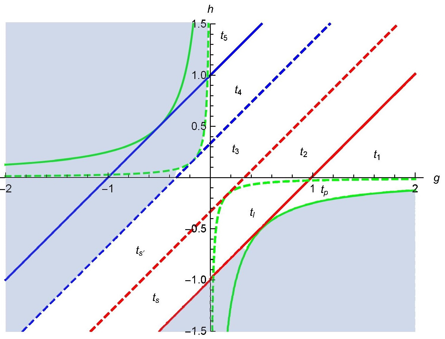
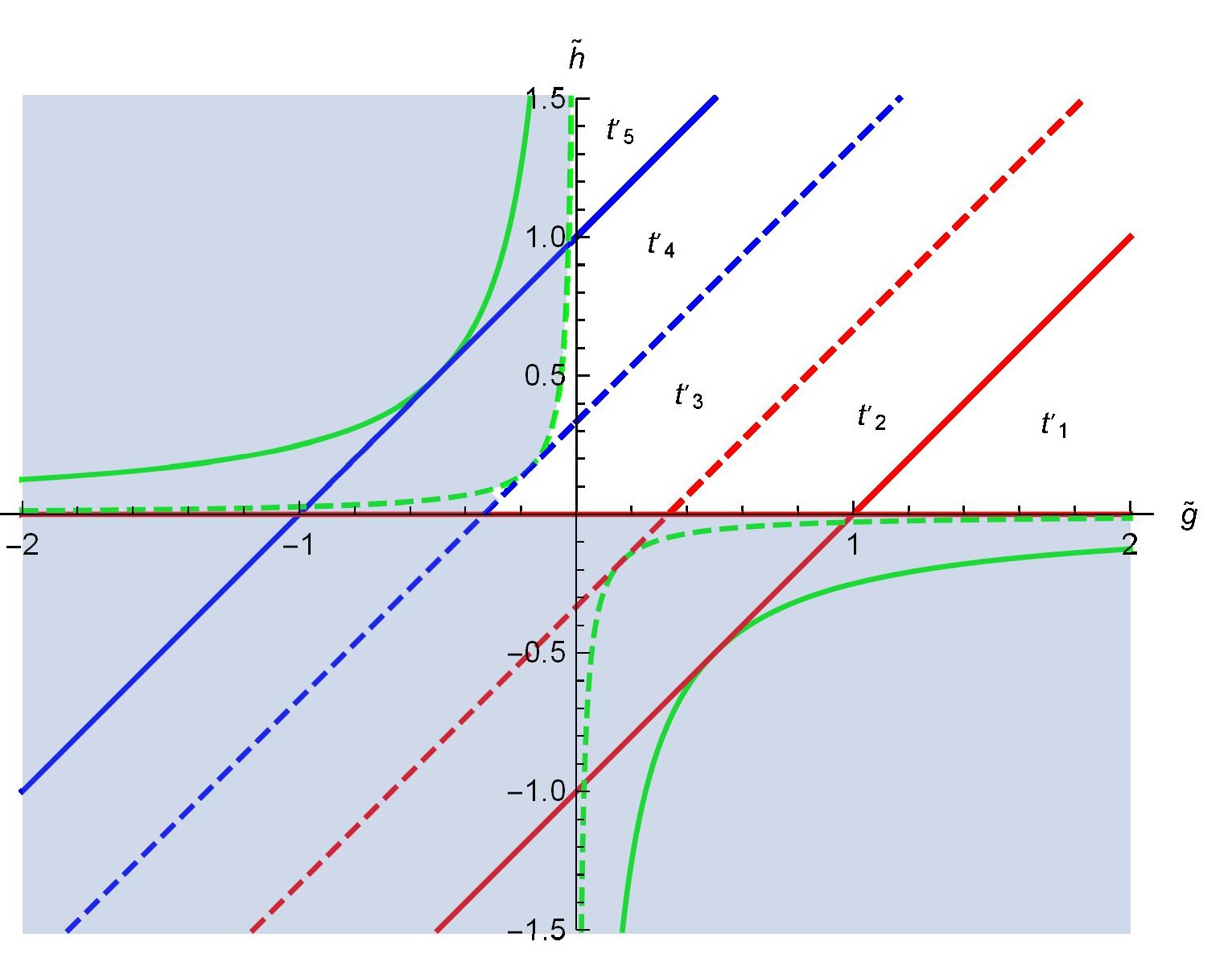
Figure 2: (a) Bifurcation diagram for two attractive centers in the plane. (b) Bifurcation diagram for two repulsive centers in the plane with the strengths (in modulus) exchanged with respect to the attractive potential. In both cases we choose α=13\alpha=\frac{1}{3}.

In Figure 2, plotted for α=1/3\alpha=1/3, we observe the bifurcation diagrams corresponding to the attractive and repulsive planar problems in Π+\Pi_{+} Fig. 2a) and Π−\Pi_{-} Fig. 2b), respectively, with strengths α1\alpha_{1}, α2\alpha_{2}, and α~1=−α2\tilde{\alpha}_{1}=-\alpha_{2}, α~2=−α1\tilde{\alpha}_{2}=-\alpha_{1}. Critical curves in both {h,g}\{h,g\} and {h~,g~}\{\tilde{h},\tilde{g}\} planes are determined by the existence of double roots in (26) and (27), see [34, 29], and shadowed areas in the diagrams are zones where motion is classically forbidden, i.e., velocities and/or momenta are imaginary.

The allowed motions in the Π+\Pi_{+}-plane are of two types: (1) If h<0h<0, orbits are bounded and are usually labeled as {ts,ts′,tl,tp}\{t_{s},t_{s^{\prime}},t_{l},t_{p}\}, for satellitary, lemniscatic and planetary ones, see [34]. (2) If h≥0h\geq 0, see [29], unbounded orbits occur, standardly labeled as {t1,t2,t3,t4,t5}\{t_{1},t_{2},t_{3},t_{4},t_{5}\}. Separatrices between bounded and unbounded motions live in the {h=0}\{h=0\} straight line.

In the Π−\Pi_{-} plane a similar, but simpler picture is found, see Fig. 2b). On the h~>0\tilde{h}>0 upper half-plane unbounded orbits exist in five different classes, labeled as {t1′,t2′,t3′,t4′,t5′}\{t^{\prime}_{1},t^{\prime}_{2},t^{\prime}_{3},t^{\prime}_{4},t^{\prime}_{5}\}. In this case the line {h~=0}\{\tilde{h}=0\} does not accommodate separatrices, but rather it corresponds to a limiting behavior of unbounded zero energy orbits reached from h~>0\tilde{h}>0.

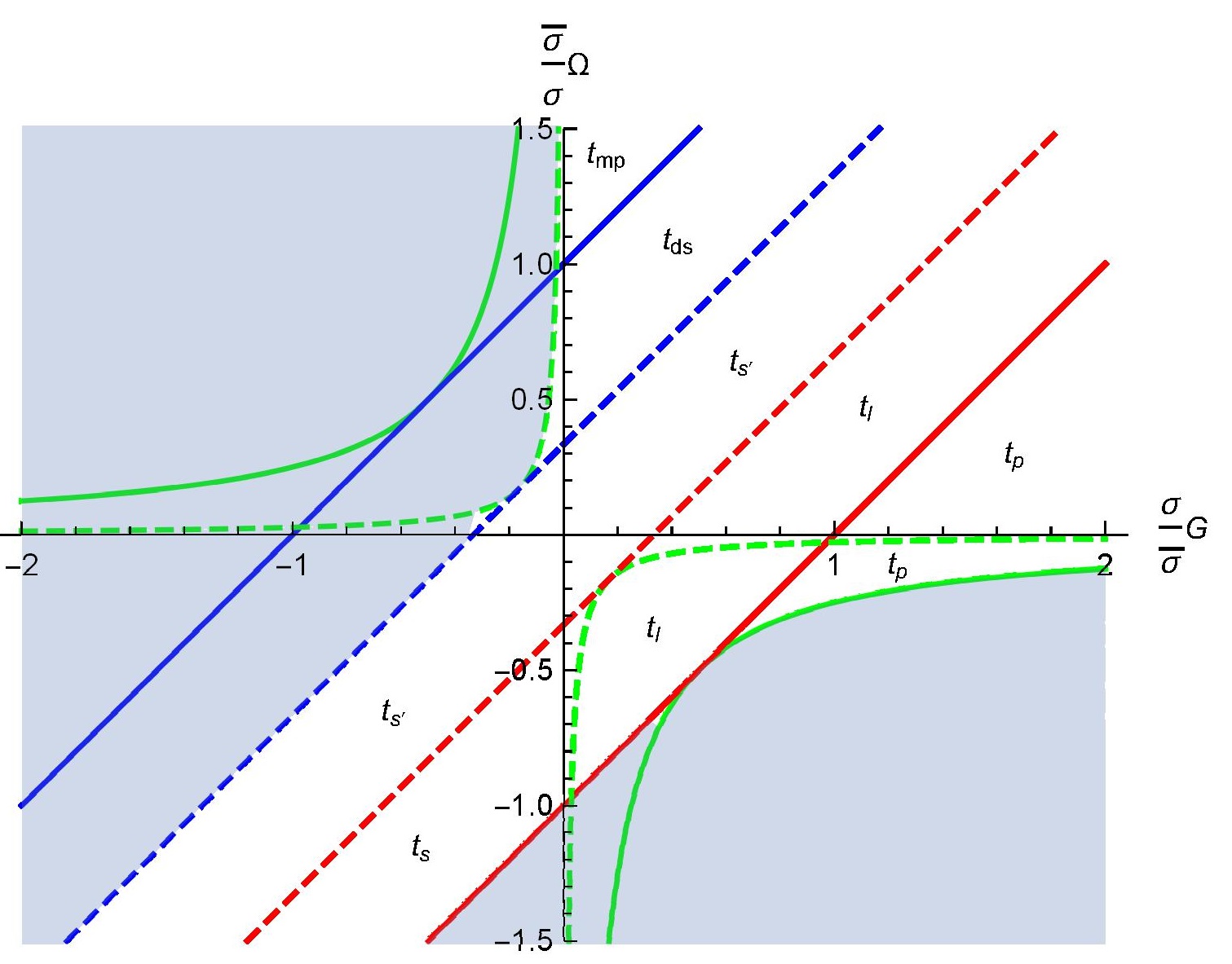
The bifurcation diagram for the complete problem in S2S^{2}, Figure 3, can now be constructed from the planar ones using transformations (24) and (25). Two morphisms are induced: (1) Orbits in Π+\Pi_{+} are mapped to orbits in S+2S^{2}_{+} identifying the invariants as follows: h=σ¯σ​Ωh=\frac{\bar{\sigma}}{\sigma}\Omega and g=σσ¯​Gg=\frac{\sigma}{\bar{\sigma}}G. (2) Orbits in Π−\Pi_{-} are mapped to orbits in S−2S^{2}_{-} if the invariants are translated to: h~=σ¯σ​Ω\tilde{h}=\frac{\bar{\sigma}}{\sigma}\Omega and g~=σσ¯​G\tilde{g}=\frac{\sigma}{\bar{\sigma}}G. The global bifurcation diagram in S2S^{2} is thus displayed on the {σ¯σ​Ω,σσ¯​G}\{\frac{\bar{\sigma}}{\sigma}\Omega,\frac{\sigma}{\bar{\sigma}}G\}-plane.

Moreover, the lower half-plane of Figure 3, σ¯σ​Ω<0\frac{\bar{\sigma}}{\sigma}\Omega<0, is mapped one-to-one with the lower half-plane of the problem of two attractive centers in Π+\Pi_{+}, Fig. 2a), as it was shown in [13], orbits lying only in S+2S_{+}^{2} are in a bijective correspondence with bounded orbits in Π+\Pi_{+}. However, with an initial condition fixed, each point (σ¯σ​Ω,σσ¯​G)\left(\frac{\bar{\sigma}}{\sigma}\Omega,\frac{\sigma}{\bar{\sigma}}G\right) in the upper half-plane of the global diagram represents an orbit that crosses the equator of S2S^{2}, and thus is mapped by (24) and (25) to the union of an unbounded orbit in Π+\Pi_{+} and another one in Π−\Pi_{-}, with equal planar energies: h=h~=σ¯σ​Ωh=\tilde{h}=\frac{\bar{\sigma}}{\sigma}\Omega.

Refer to caption

Figure 3: Global bifurcation diagram in S2S^{2} with γ=13\gamma=\frac{1}{3}.

Critical curves in Figure 3 are inherited from the corresponding ones in planar diagrams:

  • •

    Double roots in equations (26, 27) for the “radial” variable arise in the: blue straight line: ℒ12={σ¯σΩ−σσ¯G−1=0}{\cal L}_{1}^{2}=\left\{\frac{\bar{\sigma}}{\sigma}\Omega-\frac{\sigma}{\bar{\sigma}}G-1=0\right\}, red straight line: ℒ11={σ¯σΩ−σσ¯G+1=0}{\cal L}_{1}^{1}=\left\{\frac{\bar{\sigma}}{\sigma}\Omega-\frac{\sigma}{\bar{\sigma}}G+1=0\right\}, and green hyperbola: ℒ13={4ΩG+1=0}{\cal L}_{1}^{3}=\left\{4\Omega G+1=0\right\}.

  • •

    Analogously, double roots for the “angular” variable produce the: dashed blue straight line: ℒγ1={σ¯σΩ−σσ¯G−(1−2γ)=0}{\cal L}_{\gamma}^{1}=\left\{\frac{\bar{\sigma}}{\sigma}\Omega-\frac{\sigma}{\bar{\sigma}}G-(1-2\gamma)=0\right\}, dashed red straight line: ℒγ2={σ¯σΩ−σσ¯G+(1−2γ)=0}{\cal L}_{\gamma}^{2}=\left\{\frac{\bar{\sigma}}{\sigma}\Omega-\frac{\sigma}{\bar{\sigma}}G+(1-2\gamma)=0\right\}, and dashed green hyperbola: ℒγ3={4ΩG+(1−2γ)2=0}{\cal L}_{\gamma}^{3}=\left\{4\Omega G+(1-2\gamma)^{2}=0\right\}.

Orbits with Ω<0\Omega<0 are naturally labeled with the inherited standard notation for bounded motion in the planar associated problem in Π+\Pi_{+}. The branching points u1,u2u_{1},u_{2} and v1,v2v_{1},v_{2}, understood as functions of Ω\Omega and GG, allow us to specify the qualitative features of these orbits in S+2S_{+}^{2}:

  • •

    Planetary orbits (tpt_{p}). There are two analytical possibilities that lead to the same type of orbits:

    (1)\displaystyle(1) −1<1<u1<u<u2,−1<v<1,v1,v2∈ℂ,Im⁡(v1)=−Im⁡(v2)≠0\displaystyle-1<1<u_{1}<u<u_{2}\quad,\quad-1<v<1\ ,\ v_{1},v_{2}\in{\mathbb{C}},\ {\rm Im}(v_{1})=-{\rm Im}(v_{2})\neq 0 (28)
    (2)\displaystyle(2) −1<1<u1<u<u2,v1<v2<−1<v<1\displaystyle-1<1<u_{1}<u<u_{2}\quad,\quad v_{1}<v_{2}<-1<v<1 (29)

    In both cases the bounds u=u1u=u_{1} and u=u2u=u_{2} represent two caustics for these orbits, i.e., two “spherical ellipses” in the Northern hemisphere S+2S_{+}^{2}, see Fig. 6a, that confine the planetary motion of these “circumbinary” orbits.

  • •

    Lemniscatic orbits (tlt_{l}). Analogously, there exist two possibilities:

    (1)\displaystyle(1) −1<u1<1<u<u2,−1<v<1,v1,v2∈ℂ,Im⁡(v1)=−Im⁡(v2)≠0\displaystyle-1<u_{1}<1<u<u_{2}\quad,\quad-1<v<1\ ,\ v_{1},v_{2}\in{\mathbb{C}},\ {\rm Im}(v_{1})=-{\rm Im}(v_{2})\neq 0 (30)
    (2)\displaystyle(2) −1<u1<1<u<u2,v1<v2<−1<v<1.\displaystyle-1<u_{1}<1<u<u_{2}\quad,\quad v_{1}<v_{2}<-1<v<1. (31)

    A unique caustic, u=u2u=u_{2}, appears in this case. The orbits describe a lemniscatic motion around the two centers in S2+S_{2}^{+}. See Fig. 6b.

  • •

    Satellitary orbits (tst_{s}): Each point (σ¯σ​Ω,σσ¯​G)\left(\frac{\bar{\sigma}}{\sigma}\Omega,\frac{\sigma}{\bar{\sigma}}G\right) of this region in Figure 3 represents two possible orbits:

    (1)−1<u1<1<u<u2,−1<v1<v2<v<1(1)\quad-1<u_{1}<1<u<u_{2}\quad,\quad-1<v_{1}<v_{2}<v<1 (32)

    around the stronger center, limited by the caustics: u=u2u=u_{2} and v=v2v=v_{2}, and:

    (2)−1<u1<1<u<u2,−1<v<v1<v2<1(2)\quad-1<u_{1}<1<u<u_{2}\quad,\quad-1<v<v_{1}<v_{2}<1 (33)

    around the weaker center, bounded by: u=u2u=u_{2} and v=v1v=v_{1}. See Figure 6g.

  • •

    Satellitary orbits (ts′t_{s^{\prime}}) around the stronger center:

    −1<u1<1<u<u2,v1<−1<v2<v<1.-1<u_{1}<1<u<u_{2}\quad,\quad v_{1}<-1<v_{2}<v<1. (34)

    For this situation the motion is limited by the caustics: u=u2u=u_{2} and v=v2v=v_{2}, see Figure 6c.

For Ω>0\Omega>0, it is possible to extend the standard terminology, Planetary (tpt_{p}), Lemniscatic (tlt_{l}) and Satellitary (ts′t_{s^{\prime}}), to the orbits that cross the equator, but have a behavior analogous to the corresponding cases restricted to the Northern hemisphere. However, two completely new types of orbits arise. There are two zones of admissible motion without partners between the orbits with Ω<0\Omega<0, which we will call Dual Satellitary (td​st_{ds}) and Meridian Planetary (tm​pt_{mp}) orbits, taking into account its qualitative features.

Branching points are now identified by u~1=−u2\tilde{u}_{1}=-u_{2}, u~2=−u1\tilde{u}_{2}=-u_{1} and v~1=v1\tilde{v}_{1}=v_{1}, v~2=v2\tilde{v}_{2}=v_{2}, because h=h~=σ¯σ​Ωh=\tilde{h}=\frac{\bar{\sigma}}{\sigma}\Omega and g=g~=σσ¯​Gg=\tilde{g}=\frac{\sigma}{\bar{\sigma}}G in order to glue continuously the two orbit pieces on the Northern and Southern hemispheres at the equator.

  • •

    Planetary orbits (tpt_{p}): The orbits in S2S^{2} are composed by two pieces:

    S+2:\displaystyle S_{+}^{2}: u1<−1< 1<u2<u,v1<−1<v< 1<v2\displaystyle\qquad u_{1}\,<\,-1\,<\,1\,<\,u_{2}\,<\,u\ ,\qquad v_{1}\,<\,-1\,<\,v\,<\,1\,<\,v_{2} (35)
    S−2:\displaystyle S_{-}^{2}: u~1<−1< 1<u~2<u,v~1<−1<v< 1<v~2.\displaystyle\qquad\tilde{u}_{1}\,<\,-1\,<\,1\,<\,\tilde{u}_{2}\,<\,u\ ,\qquad\tilde{v}_{1}\,<\,-1\,<\,v\,<\,1\,<\,\tilde{v}_{2}.

    Note that the limit u→∞u\to\infty in both cases is nothing more than U→1U\to 1, and thus the map (24) applies two unbounded curves to a finite one that crosses the equator of S2S^{2}. The Northern pieces present the caustic: u=u2u=u_{2}, whereas the Southern ones are limited by the “spherical ellipse”: u=u~2u=\tilde{u}_{2}. The motion is confined between these curves in a planetary way and can be seen as the natural continuation of the tpt_{p} orbits in S+2S_{+}^{2} with Ω<0\Omega<0. See Figure 6d.

  • •

    Lemniscatic orbits (tlt_{l}): Analogously, there are two parts:

    S+2:\displaystyle S_{+}^{2}: u1<−1<u2< 1<u,v1<−1<v< 1<v2\displaystyle\qquad u_{1}\,<\,-1\,<\,u_{2}\,<\,1\,<\,u\ ,\qquad v_{1}\,<\,-1\,<\,v\,<\,1\,<\,v_{2} (36)
    S−2:\displaystyle S_{-}^{2}: −1<u~1< 1<u~2<u,v~1<−1<v< 1<v~2\displaystyle\qquad-1\,<\,\tilde{u}_{1}\,<\,1\,<\,\tilde{u}_{2}\,<\,u\ ,\qquad\tilde{v}_{1}\,<\,-1\,<\,v\,<\,1\,<\,\tilde{v}_{2}

    in such a way that there are no caustics in S+2S_{+}^{2} and one in S−2S_{-}^{2}: u=u~2u=\tilde{u}_{2}. We find again a natural resemblance between these orbits and their partners in the Ω<0\Omega<0 case. See Figure 6e.

  • •

    Satellitary orbits (ts′t_{s^{\prime}}):

    S+2:\displaystyle S_{+}^{2}: u1<−1<u2< 1<u,−1<v1<v< 1<v2\displaystyle\qquad u_{1}\,<\,-1\,<\,u_{2}\,<\,1\,<\,u\ ,\qquad-1\,<\,v_{1}\,<\,v\,<\,1\,<\,v_{2} (37)
    S−2:\displaystyle S_{-}^{2}: −1<u~1< 1<u~2<u,−1<v~1<v< 1<v~2.\displaystyle\qquad-1\,<\,\tilde{u}_{1}\,<\,1\,<\,\tilde{u}_{2}\,<\,u\ ,\qquad-1\,<\,\tilde{v}_{1}\,<\,v\,<\,1\,<\,\tilde{v}_{2}.

    The caustics are now: u=u~2u=\tilde{u}_{2} in S−2S_{-}^{2}, and v=v1=v~1v=v_{1}=\tilde{v}_{1} in the two hemispheres. See Figure 6f.

  • •

    Dual Satellitary orbits (td​st_{ds}):

    S+2:\displaystyle S_{+}^{2}: u1<−1<u2< 1<u,−1<v1<v<v2< 1\displaystyle\qquad u_{1}\,<\,-1\,<\,u_{2}\,<\,1\,<\,u\ ,\qquad-1\,<\,v_{1}\,<\,v\,<\,v_{2}\,<\,1 (38)
    S−2:\displaystyle S_{-}^{2}: −1<u~1< 1<u~2<u,−1<v~1<v<v~2< 1.\displaystyle\qquad-1\,<\,\tilde{u}_{1}\,<\,1\,<\,\tilde{u}_{2}\,<\,u\ ,\qquad-1\,<\,\tilde{v}_{1}\,<\,v\,<\,\tilde{v}_{2}\,<\,1.

    The td​st_{ds} orbits present a behavior delimited by the two caustics: v=v1=v~1v=v_{1}=\tilde{v}_{1} and v=v2=v~2v=v_{2}=\tilde{v}_{2} in S2S^{2}, and: u=u~2u=\tilde{u}_{2} in the Southern hemisphere. Thus, the orbits pass between the two centers in S+2S_{+}^{2}, but do not reach the South Pole. See Figure 6h.

  • •

    Meridian Planetary orbits (tm​pt_{mp}):

    S+2:\displaystyle S_{+}^{2}: −1<u1<u2< 1<u,−1<v1<v<v2< 1\displaystyle\qquad-1\,<\,u_{1}\,<\,u_{2}\,<\,1\,<\,u\ ,\qquad-1\,<\,v_{1}\,<\,v\,<\,v_{2}\,<\,1 (39)
    S−2:\displaystyle S_{-}^{2}: −1<u~1<u~2< 1<u,−1<v~1<v<v~2< 1.\displaystyle\qquad-1\,<\,\tilde{u}_{1}\,<\,\tilde{u}_{2}\,<\,1\,<\,u\ ,\qquad-1\,<\,\tilde{v}_{1}\,<\,v\,<\,\tilde{v}_{2}\,<\,1.

    The situation is similar to the td​st_{ds} case, but now only the two “angular” caustics are allowable. Thus, the orbits complete the passing between the centers not only in S+2S_{+}^{2} but also in S−2S_{-}^{2}. The tm​pt_{mp} orbits resemble the planetary ones interchanging the surrounded centers. See Figure 6i.

Finally, the analysis should be completed with the case Ω=0\Omega=0 whose orbits lie in the S+2S^{2}_{+} hemisphere. These can be easily described as the limit Ω→0\Omega\rightarrow 0 in the Ω<0\Omega<0 case. The caustic u=u2u=u_{2} for the tpt_{p}, tlt_{l} and ts′t_{s^{\prime}} orbits becomes u2→∞u_{2}\rightarrow\infty, and thus U⁡(u2)→1U(u_{2})\rightarrow 1, i.e., the equator Z=0Z=0 of S2S^{2}. Consequently, the motions are completely similar to the corresponding ones in S+2S_{+}^{2}, but now bounded by the equator.

5 Evaluation of the quadratures, inversion of the elliptic integrals

The resolution of the problem of two fixed centers has a long history that, apart from the original results of Euler [17, 18], includes the works of Lagrange [23], Legendre [24], Jacobi [20], Liouville [25] etc., see [28] and references therein. In more recent times Alexeev [6] has given a detailed qualitative analysis of the planar problem. Explicit analytical expressions determining the motion along the orbits are obtained by applying standard procedures that require the inversion of elliptic integrals, see, for instance, [15, 35]. The quadratures solving the two pairs of uncoupled ODEs (26) and (27) have been thoroughly discussed by several authors, see [28] and references therein, see also [16].

We shall briefly report here on the processes of quadrature evaluation/elliptic integral inversion in the context of the spherical problem, keeping in mind that the variables (u,v)(u,v), which appear in equations (26) and (27), should be regarded as coordinates in S+2S^{2}_{+} and S−2S^{2}_{-} through the map transformation (24), as it has been explained in the previous sections.

There are two distinctly different situations for the Ω<0\Omega<0 or Ω>0\Omega>0 ranges:

∙\bullet Ω<0\Omega<0. In this case the inversion of the elliptic integrals appearing in equations (26) is standard, we will detail only the planetary case as an example.

The range for the uu-variable in (26) (left) is: u1<u<u2u_{1}<u<u_{2}, and thus the curves: u=u1u=u_{1} and u=u2u=u_{2}, ∀v∈(−1,1)\forall v\in(-1,1), determine the two caustics. The quadrature solving the uu-equation in (26) is

±−2​σ¯σ​Ω​ζ=I⁡(u)−I⁡(u0);I⁡(u)=∫u1ud​z(z2−1)​(z−u1)​(u2−z),\pm\sqrt{-\frac{2\bar{\sigma}}{\sigma}\Omega}\,\zeta\,=\,I(u)-I(u_{0})\ ;\quad I(u)=\int_{u_{1}}^{u}\,\frac{dz}{\sqrt{(z^{2}-1)(z-u_{1})(u_{2}-z)}}, (40)

where the initial condition u⁡(0)=u0u(0)=u_{0} is assumed. The elliptic integral of the first kind I⁡(u)I(u) in (40) can be inverted by performing the following change of variable z→sz\to s, see [15] case 256:

z=u1​(1−u2)+(u2−u1)​sn2s1−u2+(u2−u1)​sn2s⇒I⁡(u)=gu​∫0su𝑑s=gu​su,z\,=\,\frac{u_{1}(1-u_{2})+(u_{2}-u_{1})\mathop{\rm sn}\nolimits^{2}s}{1-u_{2}+(u_{2}-u_{1})\mathop{\rm sn}\nolimits^{2}s}\quad\Rightarrow\quad I(u)=\,g_{u}\int_{0}^{s_{u}}\,ds\,=\,g_{u}\,s_{u},

where sns\mathop{\rm sn}\nolimits s denotes the Jacobi sinus function: sns≡sn(s|ku2)\mathop{\rm sn}\nolimits s\equiv\mathop{\rm sn}\nolimits(s|k_{u}^{2}), gug_{u} and the elliptic modulus kuk_{u} are defined in terms of the turning points as

ku2=2​(u2−u1)(u2−1)​(u1+1),gu=2(u2−1)​(u1+1).k_{u}^{2}=\frac{2(u_{2}-u_{1})}{(u_{2}-1)(u_{1}+1)}\quad,\quad g_{u}=\frac{2}{\sqrt{(u_{2}-1)(u_{1}+1)}}\,\,\,.

Formula (40) is thus simplified to become a linear relation between sus_{u} and the local time ζ\zeta which is easily inverted:

gu​(su−su0)=±−2​σ¯σ​Ω​ζ⇒su​(ζ)=±−2​σ¯σ​Ωgu​ζ+su0g_{u}\,\left(s_{u}-s_{u_{0}}\right)\,=\,\pm\sqrt{-\frac{2\bar{\sigma}}{\sigma}\Omega}\,\zeta\quad\Rightarrow\quad s_{u}(\zeta)=\frac{\pm\sqrt{-\frac{2\bar{\sigma}}{\sigma}\Omega}}{g_{u}}\,\zeta+s_{u_{0}} (41)

with: gu​su0=I⁡(u0)g_{u}s_{u_{0}}=I(u_{0}). Finally, recalling the last change of variable, the explicit inversion of (40) is achieved:

u⁡(ζ)=u1​(1−u2)+(u2−u1)​sn2su1−u2+(u2−u1)​sn2su,u(\zeta)\,=\,\frac{u_{1}(1-u_{2})+(u_{2}-u_{1})\mathop{\rm sn}\nolimits^{2}s_{u}}{1-u_{2}+(u_{2}-u_{1})\mathop{\rm sn}\nolimits^{2}s_{u}},

where sus_{u} is defined as a function of the local time ζ\zeta, su​(ζ)s_{u}(\zeta), in equation (41). Alternatively, using the properties of Jacobi elliptic functions, u⁡(ζ)u(\zeta) can be rewritten in terms of the Jacobi function dn\mathop{\rm dn}\nolimits in the simpler form:

u⁡(ζ)=u1−1+(u1+1)​dn2su1−u1+(u1+1)​dn2su,−1<1<u1<u<u2.u(\zeta)\,=\,\frac{u_{1}-1+(u_{1}+1)\mathop{\rm dn}\nolimits^{2}s_{u}}{1-u_{1}+(u_{1}+1)\mathop{\rm dn}\nolimits^{2}s_{u}}\quad,\quad-1<1<u_{1}<u<u_{2}\,. (42)

We stress, by writing the inequalities characterizing this type of orbits, that the analytic expression for u⁡(ζ)u(\zeta) appearing in formula (42) is compelled to live inside the (u1,u2)(u_{1},u_{2}) interval.

The companion expression for v⁡(ζ)v(\zeta), for instance, in the planetary case −1<v< 1-1\,<\,v\,<\,1, is given, after a completely analogous procedure, by the expressions

v⁡(ζ)=1−v2+2​v2​sn2svv2−1+2​sn2svv(\zeta)\,=\,\frac{1-v_{2}+2v_{2}\mathop{\rm sn}\nolimits^{2}s_{v}}{v_{2}-1+2\mathop{\rm sn}\nolimits^{2}s_{v}}

with

sv​(ζ)=±−2​σ¯σ​Ωgv​ζ+sv0,kv2=2​(v2−v1)(v2−1)​(1+v1),gv=2(v2−1)​(1+v1).s_{v}(\zeta)\,=\,\frac{\pm\sqrt{-\frac{2\bar{\sigma}}{\sigma}\Omega}}{g_{v}}\,\zeta\,+\,s_{v_{0}}\ ,\ k_{v}^{2}\,=\,\frac{2(v_{2}-v_{1})}{(v_{2}-1)(1+v_{1})}\ ,\ g_{v}\,=\,\frac{2}{\sqrt{(v_{2}-1)(1+v_{1})}}.

Applying transformation (24) to these expressions of u⁡(ζ)u(\zeta) and v⁡(ζ)v(\zeta) and replacing the results in (5), a complete description in Cartesian coordinates of planetary orbits in the Northern hemisphere is obtained.

Analogously, all the integrals I⁡(u)I(u) and I⁡(v)I(v) solving equations (26) in the different ranges of uu and vv compatible with Ω<0\Omega<0 can be inverted by similar techniques. The ensuing analytic expressions are assembled in the Appendix. The u⁡(ζ)u(\zeta) and v⁡(ζ)v(\zeta) functions which, respectively, solve the uu- and vv-dynamics are smooth, bounded between turning points, and periodic with periods, respectively, Tu∝K⁡(ku2)T_{u}\propto K(k_{u}^{2}) and Tv∝K⁡(kv2)T_{v}\propto K(k_{v}^{2}), where K⁡(k2)K(k^{2}) is the complete elliptic function of the first kind. The trajectories in all these cases are bounded between caustics in S+2S^{2}_{+} and dense, except if the uu- and vv-periods are commensurable.

∙\bullet Ω>0\Omega>0. The procedure is more delicate in this case essentially because the trajectories complying with the ODE pair (26) reach the equator, whereas there is admissible motion governed by (27) that also reaches the equator coming from the Southern hemisphere. Therefore, it is convenient to investigate the inversion of the quadratures of the uu-equations of both (26) and (27) in a global form. However, in the “angular”vv-integrals there are no differences with respect to the Ω<0\Omega<0 range.

Let us focus on planetary orbits. An orbit of this type in S2S^{2} is described by two pieces: the portion belonging to S+2S_{+}^{2} is a solution of equations (26) in the ranges

u1<−1< 1<u2<u,v1<−1<v< 1<v2,u_{1}\,<\,-1\,<\,1\,<\,u_{2}\,<\,u\ ,\qquad v_{1}\,<\,-1\,<\,v\,<\,1\,<\,v_{2},

whereas for the S−2S_{-}^{2} piece we have equations (27) and the ranges

u~1<−1< 1<u~2<u,v~1<−1<v< 1<v~2.\tilde{u}_{1}\,<\,-1\,<\,1\,<\,\tilde{u}_{2}\,<\,u\ ,\qquad\tilde{v}_{1}\,<\,-1\,<\,v\,<\,1\,<\,\tilde{v}_{2}.

The first quadrature in (26) for the “radial” variable

±2​σ¯σ​Ω​ζ=I⁡(u)−I⁡(u0);I⁡(u)=∫u2ud​z(z2−1)​(z−u1)​(z−u2)\pm\sqrt{\frac{2\bar{\sigma}}{\sigma}\Omega}\,\zeta\,=\,I(u)-I(u_{0})\ ;\quad I(u)=\int_{u_{2}}^{u}\,\frac{dz}{\sqrt{(z^{2}-1)(z-u_{1})(z-u_{2})}}\,\,\, (43)

can be inverted with a change of variable like that explained before in the Ω<0\Omega<0 case. The solution is

u⁡(ζ)≡u⁡(su)=u2−1+(u2+1)​dn2su1−u2+(u2+1)​dn2su,u(\zeta)\equiv u(s_{u})=\frac{u_{2}-1+(u_{2}+1)\mathop{\rm dn}\nolimits^{2}s_{u}}{1-u_{2}+(u_{2}+1)\mathop{\rm dn}\nolimits^{2}s_{u}}, (44)

where

su​(ζ)=±2​σ¯σ​Ωgu​ζ+su0,ku2=2​(u2−u1)(1−u1)​(1+u2),gu=2(1−u1)​(1+u2).s_{u}(\zeta)=\,\frac{\pm\sqrt{\frac{2\bar{\sigma}}{\sigma}\Omega}}{g_{u}}\,\zeta+s_{u_{0}}\ ,\ k_{u}^{2}=\frac{2(u_{2}-u_{1})}{(1-u_{1})(1+u_{2})}\ ,\ g_{u}=\frac{2}{\sqrt{(1-u_{1})(1+u_{2})}}.

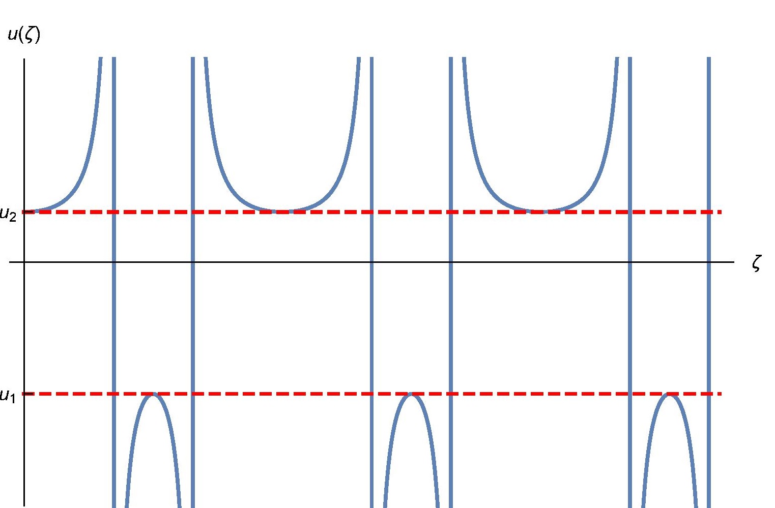
A plot of u⁡(ζ)u(\zeta), see Figure 4a, shows several relevant features of u⁡(ζ)u(\zeta). First, the function (44) presents infinite poles located at the points where dn2su=u2−1u2+1\mathop{\rm dn}\nolimits^{2}s_{u}=\frac{u_{2}-1}{u_{2}+1}. This is an expected result if one sees u⁡(ζ)u(\zeta) as a solution of the planar problem of two attractive centers with h>0h>0 reinterpreting ζ\zeta as the local time of this planar problem; the trajectory goes to infinity in a finite interval of the local time. However, in the sphere S2S^{2} the sphero-conical variable U⁡(ζ)U(\zeta), given by (24), is bounded but exhibits finite discontinuities and reaches its maxima on the equator U=1U=1 at the poles of u⁡(ζ)u(\zeta), see Fig. 4b. Second, it is remarkable, and a priori unexpected, that both u⁡(ζ)u(\zeta) and U⁡(ζ)U(\zeta) take negative values. The subtle interpretation of this fact is the understanding that, given the inversion problem posed by (43), its solution u⁡(ζ)≡u⁡(su)u(\zeta)\equiv u(s_{u}) solves also the complementary problem: y<u1<−1<1<u2y<u_{1}<-1<1<u_{2}, i.e., the inversion problem of the elliptic integral:

I′​(y)=∫yu1d​z(z2−1)​(z−u1)​(z−u2)I^{\prime}(y)=\int_{y}^{u_{1}}\frac{dz}{\sqrt{(z^{2}-1)(z-u_{1})(z-u_{2})}}

in such a way that the inverse function y⁡(s)y(s) verifies: y⁡(s)=u⁡(su+K)y(s)=u(s_{u}+K), where K=K⁡(ku2)K=K(k_{u}^{2}). Thus, u⁡(su)u(s_{u}) defined in equation (44) represents simultaneously the genuine uu-“radial”positive solution, u∈(u2,∞)u\in(u_{2},\infty), and the negative y⁡(s)y(s)-“radial”solution with y∈(−∞,u1)y\in(-\infty,u_{1}). Note that, according to the plot in Figure 4, these two solutions occur in consecutive intervals of the local time ζ\zeta.

Refer to caption  Refer to caption

Figure 4: (a) Graphics of the function u⁡(ζ)u(\zeta) defined in (44) and (b) its partner U⁡(ζ)U(\zeta) in S2S^{2}, corresponding to the values: Ω=3\Omega=\sqrt{3}, G=2​33G=\frac{2\sqrt{3}}{3}, σ=cos⁡π6\sigma=\cos\frac{\pi}{6}, su0=0s_{u_{0}}=0.

Refer to caption

Figure 5: Graphics of the function |U⁡(ζ)||U(\zeta)| corresponding to the values: Ω=3\Omega=\sqrt{3}, G=2​33G=\frac{2\sqrt{3}}{3}, σ=cos⁡π6\sigma=\cos\frac{\pi}{6}, su0=0s_{u_{0}}=0.

A direct search for the solution of equation (27) in S−2S^{2}_{-}, where u~1<−1<1<u~2<u\tilde{u}_{1}<-1<1<\tilde{u}_{2}<u, requires the inversion of the elliptic integral in the following equation:

±2​σ¯σ​Ω​ζ=I~​(u)−I~​(u0),I~​(u)=∫u~2ud​z(z2−1)​(z−u~1)​(z−u~2).\pm\sqrt{\frac{2\bar{\sigma}}{\sigma}\Omega}\,\zeta\,=\,\tilde{I}(u)-\tilde{I}(u_{0})\ ,\quad\tilde{I}(u)=\int_{\tilde{u}_{2}}^{u}\,\frac{dz}{\sqrt{(z^{2}-1)(z-\tilde{u}_{1})(z-\tilde{u}_{2})}}\,\,\,.

Having in mind that u~1=−u2\tilde{u}_{1}=-u_{2}, u~2=−u1\tilde{u}_{2}=-u_{1}, we can write

I~​(u)=∫−u1ud​z(z2−1)​(z+u2)​(z+u1)=∫−uu1d​w(w2−1)​(w−u2)​(w−u1)=I′​(−u),\tilde{I}(u)=\int_{-u_{1}}^{u}\,\frac{dz}{\sqrt{(z^{2}-1)(z+u_{2})(z+u_{1})}}=\int_{-u}^{u_{1}}\,\frac{dw}{\sqrt{(w^{2}-1)(w-u_{2})(w-u_{1})}}=I^{\prime}(-u),

where the change of variable z=−wz=-w has been performed. Thus, we conclude that the inversion of I~​(u)\tilde{I}(u), i.e., the “radial” solution in S−2S^{2}_{-}, is tantamount to the inversion of I′​(−u)I^{\prime}(-u) and consequently to minus the negative part of u⁡(su)u(s_{u}) given in (44). Therefore, we represent the “radial” solution simultaneously in both S+2S^{2}_{+} and S−2S^{2}_{-} by simply taking the absolute value |u⁡(ζ)||u(\zeta)| of the solution given in (44). Moreover, with this identification the function |U⁡(ζ)||U(\zeta)| is smooth, i.e., the gluing at the equator of the Northern and Southern branches of the orbits is continuous and differentiable, see Figure 5, with respect to the local time ζ\zeta.

This argument is valid also for the “radial” quadratures of the rest of different types of orbits that cross the equator. Thus, the general expression for the orbits in Cartesian coordinates over the sphere S2S^{2}, using (24) in (5), can be written in a compact form valid for all the types of orbits described in the previous section as

X⁡(ζ)\displaystyle X(\zeta) =\displaystyle= R​σ¯|u⁡(ζ)|v⁡(ζ)σ¯2​u2​(ζ)+σ2​σ¯2​v2​(ζ)+σ2\displaystyle\frac{R\bar{\sigma}\,|u(\zeta)|\,v(\zeta)}{\sqrt{\bar{\sigma}^{2}u^{2}(\zeta)+\sigma^{2}}\sqrt{\bar{\sigma}^{2}v^{2}(\zeta)+\sigma^{2}}}
Y⁡(ζ)\displaystyle Y(\zeta) =\displaystyle= ±R​σ​σ¯​u2​(ζ)−1​1−v2​(ζ)σ¯2​u2​(ζ)+σ2​σ¯2​v2​(ζ)+σ2\displaystyle\frac{\pm R\sigma\bar{\sigma}\,\sqrt{u^{2}(\zeta)-1}\,\sqrt{1-v^{2}(\zeta)}}{\sqrt{\bar{\sigma}^{2}u^{2}(\zeta)+\sigma^{2}}\sqrt{\bar{\sigma}^{2}v^{2}(\zeta)+\sigma^{2}}} (45)
Z⁡(ζ)\displaystyle Z(\zeta) =\displaystyle= R​σ​sg​[u⁡(ζ)]σ¯2​u2​(ζ)+σ2​σ¯2​v2​(ζ)+σ2.\displaystyle\frac{R\sigma\,\mathrm{sg}[u(\zeta)]}{\sqrt{\bar{\sigma}^{2}u^{2}(\zeta)+\sigma^{2}}\sqrt{\bar{\sigma}^{2}v^{2}(\zeta)+\sigma^{2}}}\,\,\,.

Here, sg\mathrm{sg} denotes the sign function and (u⁡(ζ),v⁡(ζ))(u(\zeta),v(\zeta)) are the solutions of equations (22) or (23).

Explicit expressions for (45) in all the different regimes are written in the Appendix.

The quasiperiodicity properties of the functions (45) are inherited from the Jacobi elliptic functions through the functions u⁡(ζ)u(\zeta) and v⁡(ζ)v(\zeta): solutions (45) are products of periodic functions with different periods TuT_{u} and TvT_{v}. Consequently, (45) will be periodic, and thus the orbits will be closed, only if TuT_{u} and TvT_{v} are commensurable, i.e., there exists p,q∈ℕ∗p,q\in\mathbb{N}^{*} such that

p​Tu=q​Tv,p\,T_{u}\,=\,q\,T_{v}, (46)

otherwise the orbits will be dense inside the allowable region of S2S^{2}.

The periods TuT_{u} and TvT_{v} are proportional to K⁡(ku2)K(k_{u}^{2}) and K⁡(kv2)K(k_{v}^{2}), respectively, with a factor that depends on the concrete Jacobi functions involved in the respective expressions of u⁡(ζ)u(\zeta) and v⁡(ζ)v(\zeta). The search for a closed orbit, with the values of pp, qq and Ω\Omega (or GG) fixed, requires that the transcendental equation (46) be solved in the variable GG (alternatively Ω\Omega). Explicit expressions for the periods and concrete examples of closed orbits for different values of pp and qq are collected in the Appendix.

Acknowledgments

The authors thank the Spanish Ministerio de Economía y Competitividad (MINECO) for financial support under grant MTM2014-57129-C2-1-P and the Junta de Castilla y León grant VA057U16.

Appendix. Explicit expressions for different types of orbits

The set of parameters that determines the problem is RR, θf\theta_{f}, γ1\gamma_{1} and γ2\gamma_{2}, but after defining nondimensional variables the strengths can be measured with only one relative quantity: γ=γ2γ1+γ2\gamma=\frac{\gamma_{2}}{\gamma_{1}+\gamma_{2}}.

Our choice of integration constants to characterize the solutions (45) as functions of the nondimensional local time ζ\zeta introduced in (25) is: the two constants of motion Ω\Omega and GG and the two initial data su0s_{u_{0}} and sv0s_{v_{0}}. The dependence in Ω\Omega and GG is given implicitly through the values of the branching points:

u1\displaystyle u_{1} =\displaystyle= σσ¯​[−12​Ω−GΩ+14​Ω2],u2=σσ¯​[−12​Ω+GΩ+14​Ω2]\displaystyle\frac{\sigma}{\bar{\sigma}}\left[\frac{-1}{2\Omega}-\sqrt{\frac{G}{\Omega}+\frac{1}{4\Omega^{2}}}\right]\qquad\quad,\quad\qquad u_{2}=\frac{\sigma}{\bar{\sigma}}\left[\frac{-1}{2\Omega}+\sqrt{\frac{G}{\Omega}+\frac{1}{4\Omega^{2}}}\right]
v1\displaystyle v_{1} =\displaystyle= σσ¯​[(1−2​γ)2​Ω−GΩ+(1−2​γ)24​Ω2],v2=σσ¯​[(1−2​γ)2​Ω+GΩ+(1−2​γ)24​Ω2]\displaystyle\frac{\sigma}{\bar{\sigma}}\left[\frac{(1-2\gamma)}{2\Omega}-\sqrt{\frac{G}{\Omega}+\frac{(1-2\gamma)^{2}}{4\Omega^{2}}}\right]\ ,\ v_{2}=\frac{\sigma}{\bar{\sigma}}\left[\frac{(1-2\gamma)}{2\Omega}+\sqrt{\frac{G}{\Omega}+\frac{(1-2\gamma)^{2}}{4\Omega^{2}}}\right]

if Ω≠0\Omega\neq 0, and u1=σσ¯​Gu_{1}=\frac{\sigma}{\bar{\sigma}}G, v2=σσ¯​−G(1−2​γ)v_{2}=\frac{\sigma}{\bar{\sigma}}\,\frac{-G}{(1-2\gamma)} for the Ω=0\Omega=0 case.

Remember also that the following notation has been introduced throughout the paper:

σ=cos⁡θf,σ¯=sin⁡θf;snsu=sn(su​(ζ)|ku2),\sigma=\cos\theta_{f}\ ,\quad\bar{\sigma}=\sin\theta_{f}\ ;\quad\mathop{\rm sn}\nolimits s_{u}=\mathop{\rm sn}\nolimits(s_{u}(\zeta)|k_{u}^{2}),

and so on for the rest of the Jacobi elliptic functions, where

su≡su​(ζ)=±2​σ¯σ​|Ω|gu​ζ+su0,sv≡sv​(ζ)=±2​σ¯σ​|Ω|gv​ζ+sv0if​Ω≠0\displaystyle s_{u}\equiv s_{u}(\zeta)=\frac{\pm\sqrt{\frac{2\bar{\sigma}}{\sigma}|\Omega|}}{g_{u}}\,\zeta+s_{u_{0}}\ ,\quad s_{v}\equiv s_{v}(\zeta)=\frac{\pm\sqrt{\frac{2\bar{\sigma}}{\sigma}|\Omega|}}{g_{v}}\,\zeta+s_{v_{0}}\qquad{\rm if}\ \Omega\neq 0
su≡su​(ζ)=±2gu​ζ+su0,sv≡sv​(ζ)=±2gv​ζ+sv0if​Ω=0\displaystyle s_{u}\equiv s_{u}(\zeta)=\frac{\pm\sqrt{2}}{g_{u}}\,\zeta+s_{u_{0}}\ ,\qquad s_{v}\equiv s_{v}(\zeta)=\frac{\pm\sqrt{2}}{g_{v}}\,\zeta+s_{v_{0}}\qquad{\rm if}\ \Omega=0

in such a way that the initial conditions are su0=su​(0)s_{u_{0}}=s_{u}(0) and sv0=sv​(0)s_{v_{0}}=s_{v}(0).

With all these considerations, the orbits for the two fixed centers problem in S2S^{2} are:


Ω>0\Omega>0: Orbits that cross the equator.


∙\bullet Planetary orbits-tpt_{p}, see (35):

{X⁡(ζ)=RΥu​Υv​σ¯​(1−u2−(u2+1)​dn2​su)​(1−v1+2​v1​sn2​sv)Y⁡(ζ)=RΥu​Υv​ 4​σ​σ¯​u22−1​v12−1​dn​su​sn​sv​cn​svZ⁡(ζ)=RΥu​Υv​σ​(u2−1−(u2+1)​dn2​su)​(v1−1+2​sn2​sv)\left\{\begin{array}[]{l}X(\zeta)=\frac{R}{\Upsilon_{u}\Upsilon_{v}}\,\bar{\sigma}\,(1-u_{2}-(u_{2}+1)\,{\rm dn}^{2}s_{u})\,(1-v_{1}+2v_{1}\,{\rm sn}^{2}s_{v})\\ \\ Y(\zeta)=\frac{R}{\Upsilon_{u}\Upsilon_{v}}\,4\sigma\bar{\sigma}\,\sqrt{u_{2}^{2}-1}\,\sqrt{v_{1}^{2}-1}\ {\rm dn}s_{u}\,{\rm sn}s_{v}\,{\rm cn}s_{v}\\ \\ Z(\zeta)=\frac{R}{\Upsilon_{u}\Upsilon_{v}}\,\sigma\,(u_{2}-1-(u_{2}+1)\,{\rm dn}^{2}s_{u})\,(v_{1}-1+2\,{\rm sn}^{2}s_{v})\end{array}\right. (47)

where

Υu\displaystyle\Upsilon_{u} =\displaystyle= (u2−1)2−2​(u22−1)​(σ2−σ¯2)​dn2​su+(u2+1)2​dn4​su\displaystyle\sqrt{(u_{2}-1)^{2}-2(u_{2}^{2}-1)(\sigma^{2}-\bar{\sigma}^{2})\,{\rm dn}^{2}s_{u}+(u_{2}+1)^{2}\,{\rm dn}^{4}s_{u}}
Υv\displaystyle\Upsilon_{v} =\displaystyle= (v1−1)2+4​(1−v1)​(σ¯2​v1−σ2)​sn2​sv+4​(σ¯2​v12+σ2)​sn4​sv\displaystyle\sqrt{(v_{1}-1)^{2}+4(1-v_{1})(\bar{\sigma}^{2}v_{1}-\sigma^{2})\,{\rm sn}^{2}s_{v}+4(\bar{\sigma}^{2}v_{1}^{2}+\sigma^{2})\,{\rm sn}^{4}s_{v}}
ku2=2​(u2−u1)(1−u1)​(1+u2),gu=2(1−u1)​(1+u2),kv2=2​(v2−v1)(1−v1)​(1+v2),gv=2(1−v1)​(1+v2)k_{u}^{2}=\frac{2(u_{2}-u_{1})}{(1-u_{1})(1+u_{2})}\ ,\ g_{u}=\frac{2}{\sqrt{(1-u_{1})(1+u_{2})}}\ ,\ k_{v}^{2}=\frac{2(v_{2}-v_{1})}{(1-v_{1})(1+v_{2})}\ ,\ g_{v}=\frac{2}{\sqrt{(1-v_{1})(1+v_{2})}}

∙\bullet Lemniscatic orbits-tlt_{l} (36):

{X⁡(ζ)=RΥu​Υv​σ¯​(u2−1−2​u2​dn2​su)​(1−v1+2​v1​sn2​sv)Y⁡(ζ)=RΥu​Υv​ 4​σ​σ¯​ku​1−u22​v12−1​dn​su​sn​su​sn​sv​cn​svZ⁡(ζ)=RΥu​Υv​σ​(1−u2−2​dn2​su)​(v1−1+2​sn2​sv)\left\{\begin{array}[]{l}X(\zeta)=\frac{R}{\Upsilon_{u}\Upsilon_{v}}\,\bar{\sigma}\,(u_{2}-1-2u_{2}\,{\rm dn}^{2}s_{u})\,(1-v_{1}+2v_{1}\,{\rm sn}^{2}s_{v})\\ \\ Y(\zeta)=\frac{R}{\Upsilon_{u}\Upsilon_{v}}\,4\sigma\bar{\sigma}\,k_{u}\,\sqrt{1-u_{2}^{2}}\,\sqrt{v_{1}^{2}-1}\ {\rm dn}s_{u}\,{\rm sn}s_{u}\,{\rm sn}s_{v}\,{\rm cn}s_{v}\\ \\ Z(\zeta)=\frac{R}{\Upsilon_{u}\Upsilon_{v}}\,\sigma\,(1-u_{2}-2\,{\rm dn}^{2}s_{u})\,(v_{1}-1+2\,{\rm sn}^{2}s_{v})\end{array}\right. (48)
Υu\displaystyle\Upsilon_{u} =\displaystyle= (u2−1)2+4​(1−u2)​(σ¯2​u2−σ2)​dn2​su+4​(σ¯2​u22+σ2)​dn4​su\displaystyle\sqrt{(u_{2}-1)^{2}+4(1-u_{2})(\bar{\sigma}^{2}u_{2}-\sigma^{2})\,{\rm dn}^{2}s_{u}+4(\bar{\sigma}^{2}u_{2}^{2}+\sigma^{2})\,{\rm dn}^{4}s_{u}}
Υv\displaystyle\Upsilon_{v} =\displaystyle= (v1−1)2+4​(1−v1)​(σ¯2​v1−σ2)​sn2​sv+4​(σ¯2​v12+σ2)​sn4​sv\displaystyle\sqrt{(v_{1}-1)^{2}+4(1-v_{1})(\bar{\sigma}^{2}v_{1}-\sigma^{2})\,{\rm sn}^{2}s_{v}+4(\bar{\sigma}^{2}v_{1}^{2}+\sigma^{2})\,{\rm sn}^{4}s_{v}}
ku2=(1−u1)​(1+u2)2​(u2−u1),gu=2u2−u1,kv2=2​(v2−v1)(1−v1)​(1+v2),gv=2(1−v1)​(1+v2)k_{u}^{2}=\frac{(1-u_{1})(1+u_{2})}{2(u_{2}-u_{1})}\ ,\ g_{u}=\frac{\sqrt{2}}{\sqrt{u_{2}-u_{1}}}\ ,\ k_{v}^{2}=\frac{2(v_{2}-v_{1})}{(1-v_{1})(1+v_{2})}\ ,\ g_{v}=\frac{2}{\sqrt{(1-v_{1})(1+v_{2})}}

∙\bullet Satellitary orbits-ts′t_{s^{\prime}} (37):

{X⁡(ζ)=RΥu​Υv​σ¯​(1−u2+2​u2​dn2​su)​(2​v1+(1−v1)​sn2​sv)Y⁡(ζ)=RΥu​Υv​ 4​σ​σ¯​ku​1−u22​1−v12​dn​su​sn​su​cn​svZ⁡(ζ)=RΥu​Υv​σ​(u2−1+2​dn2​su)​(2−(1−v1)​sn2​sv)\left\{\begin{array}[]{l}X(\zeta)=\frac{R}{\Upsilon_{u}\Upsilon_{v}}\,\bar{\sigma}\,(1-u_{2}+2u_{2}\,{\rm dn}^{2}s_{u})\,(2v_{1}+(1-v_{1})\,{\rm sn}^{2}s_{v})\\ \\ Y(\zeta)=\frac{R}{\Upsilon_{u}\Upsilon_{v}}\,4\sigma\bar{\sigma}\,k_{u}\,\sqrt{1-u_{2}^{2}}\,\sqrt{1-v_{1}^{2}}\ {\rm dn}s_{u}\,{\rm sn}s_{u}\,{\rm cn}s_{v}\\ \\ Z(\zeta)=\frac{R}{\Upsilon_{u}\Upsilon_{v}}\,\sigma\,(u_{2}-1+2\,{\rm dn}^{2}s_{u})\,(2-(1-v_{1})\,{\rm sn}^{2}s_{v})\end{array}\right. (49)
Υu\displaystyle\Upsilon_{u} =\displaystyle= (u2−1)2+4​(1−u2)​(σ¯2​u2−σ2)​dn2​su+4​(σ¯2​u22+σ2)​dn4​su\displaystyle\sqrt{(u_{2}-1)^{2}+4(1-u_{2})(\bar{\sigma}^{2}u_{2}-\sigma^{2})\,{\rm dn}^{2}s_{u}+4(\bar{\sigma}^{2}u_{2}^{2}+\sigma^{2})\,{\rm dn}^{4}s_{u}}
Υv\displaystyle\Upsilon_{v} =\displaystyle= 4​(σ¯2​v12+σ2)+4​(1−v1)​(σ¯2​v1−σ2)​sn2​sv+(v1−1)2​sn4​sv\displaystyle\sqrt{4(\bar{\sigma}^{2}v_{1}^{2}+\sigma^{2})+4(1-v_{1})(\bar{\sigma}^{2}v_{1}-\sigma^{2})\,{\rm sn}^{2}s_{v}+(v_{1}-1)^{2}\,{\rm sn}^{4}s_{v}}
ku2=(1−u1)​(1+u2)2​(u2−u1),gu=2u2−u1,kv2=(1−v1)​(1+v2)2​(v2−v1),gv=2v2−v1k_{u}^{2}=\frac{(1-u_{1})(1+u_{2})}{2(u_{2}-u_{1})}\ ,\ g_{u}=\frac{\sqrt{2}}{\sqrt{u_{2}-u_{1}}}\ ,\ k_{v}^{2}=\frac{(1-v_{1})(1+v_{2})}{2(v_{2}-v_{1})}\ ,\ g_{v}=\frac{\sqrt{2}}{\sqrt{v_{2}-v_{1}}}

∙\bullet Dual Satellitary orbits-td​st_{ds} (38):

{X⁡(ζ)=RΥu​Υv​σ¯​(1−u2+2​u2​dn2​su)​(1+v1−(1−v1)​dn2​sv)Y⁡(ζ)=RΥu​Υv​ 4​σ​σ¯​ku​1−u22​1−v12​dn​su​sn​su​dn​svZ⁡(ζ)=RΥu​Υv​σ​(u2−1+2​dn2​su)​(1+v1+(1−v1)​dn2​sv)\left\{\begin{array}[]{l}X(\zeta)=\frac{R}{\Upsilon_{u}\Upsilon_{v}}\,\bar{\sigma}\,(1-u_{2}+2u_{2}\,{\rm dn}^{2}s_{u})\,(1+v_{1}-(1-v_{1})\,{\rm dn}^{2}s_{v})\\ \\ Y(\zeta)=\frac{R}{\Upsilon_{u}\Upsilon_{v}}\,4\sigma\bar{\sigma}\,k_{u}\,\sqrt{1-u_{2}^{2}}\,\sqrt{1-v_{1}^{2}}\ {\rm dn}s_{u}\,{\rm sn}s_{u}\,{\rm dn}s_{v}\\ \\ Z(\zeta)=\frac{R}{\Upsilon_{u}\Upsilon_{v}}\,\sigma\,(u_{2}-1+2\,{\rm dn}^{2}s_{u})\,(1+v_{1}+(1-v_{1})\,{\rm dn}^{2}s_{v})\end{array}\right. (50)
Υu\displaystyle\Upsilon_{u} =\displaystyle= (u2−1)2+4​(1−u2)​(σ¯2​u2−σ2)​dn2​su+4​(σ¯2​u22+σ2)​dn4​su\displaystyle\sqrt{(u_{2}-1)^{2}+4(1-u_{2})(\bar{\sigma}^{2}u_{2}-\sigma^{2})\,{\rm dn}^{2}s_{u}+4(\bar{\sigma}^{2}u_{2}^{2}+\sigma^{2})\,{\rm dn}^{4}s_{u}}
Υv\displaystyle\Upsilon_{v} =\displaystyle= (1+v1)2+2​(1−v12)​(σ2−σ¯2)​dn2​sv+(1−v1)2​dn4​sv\displaystyle\sqrt{(1+v_{1})^{2}+2(1-v_{1}^{2})(\sigma^{2}-\bar{\sigma}^{2})\,{\rm dn}^{2}s_{v}+(1-v_{1})^{2}\,{\rm dn}^{4}s_{v}}
ku2=(1−u1)​(1+u2)2​(u2−u1),gu=2u2−u1,kv2=2​(v2−v1)(1−v1)​(1+v2),gv=2(1−v1)​(1+v2)k_{u}^{2}=\frac{(1-u_{1})(1+u_{2})}{2(u_{2}-u_{1})}\ ,\ g_{u}=\frac{\sqrt{2}}{\sqrt{u_{2}-u_{1}}}\ ,\ k_{v}^{2}=\frac{2(v_{2}-v_{1})}{(1-v_{1})(1+v_{2})}\ ,\ g_{v}=\frac{2}{\sqrt{(1-v_{1})(1+v_{2})}}

∙\bullet Meridian Planetary orbits-tm​pt_{mp} (39):

{X⁡(ζ)=RΥu​Υv​σ¯​(u2+1−2​u2​sn2​su)​(1+v1−(1−v1)​dn2​sv)Y⁡(ζ)=RΥu​Υv​ 4​σ​σ¯​1−u22​1−v12​cn​su​sn​su​dn​svZ⁡(ζ)=RΥu​Υv​σ​(1+u2−2​sn2​su)​(1+v1+(1−v1)​dn2​sv)\left\{\begin{array}[]{l}X(\zeta)=\frac{R}{\Upsilon_{u}\Upsilon_{v}}\,\bar{\sigma}\,(u_{2}+1-2u_{2}\,{\rm sn}^{2}s_{u})\,(1+v_{1}-(1-v_{1})\,{\rm dn}^{2}s_{v})\\ \\ Y(\zeta)=\frac{R}{\Upsilon_{u}\Upsilon_{v}}\,4\sigma\bar{\sigma}\,\sqrt{1-u_{2}^{2}}\,\sqrt{1-v_{1}^{2}}\ {\rm cn}s_{u}\,{\rm sn}s_{u}\,{\rm dn}s_{v}\\ \\ Z(\zeta)=\frac{R}{\Upsilon_{u}\Upsilon_{v}}\,\sigma\,(1+u_{2}-2\,{\rm sn}^{2}s_{u})\,(1+v_{1}+(1-v_{1})\,{\rm dn}^{2}s_{v})\end{array}\right. (51)
Υu\displaystyle\Upsilon_{u} =\displaystyle= (1+u2)2−4​(1+u2)​(σ¯2​u2+σ2)​sn2​su+4​(σ¯2​u22+σ2)​sn4​su\displaystyle\sqrt{(1+u_{2})^{2}-4(1+u_{2})(\bar{\sigma}^{2}u_{2}+\sigma^{2})\,{\rm sn}^{2}s_{u}+4(\bar{\sigma}^{2}u_{2}^{2}+\sigma^{2})\,{\rm sn}^{4}s_{u}}
Υv\displaystyle\Upsilon_{v} =\displaystyle= (1+v1)2+2​(1−v12)​(σ2−σ¯2)​dn2​sv+(1−v1)2​dn4​sv\displaystyle\sqrt{(1+v_{1})^{2}+2(1-v_{1}^{2})(\sigma^{2}-\bar{\sigma}^{2})\,{\rm dn}^{2}s_{v}+(1-v_{1})^{2}\,{\rm dn}^{4}s_{v}}
ku2=2​(u2−u1)(1−u1)​(1+u2),gu=2(1−u1)​(1+u2),kv2=2​(v2−v1)(1−v1)​(1+v2),gv=2(1−v1)​(1+v2)k_{u}^{2}=\frac{2(u_{2}-u_{1})}{(1-u_{1})(1+u_{2})}\ ,\ g_{u}=\frac{2}{\sqrt{(1-u_{1})(1+u_{2})}}\ ,\ k_{v}^{2}=\frac{2(v_{2}-v_{1})}{(1-v_{1})(1+v_{2})}\ ,\ g_{v}=\frac{2}{\sqrt{(1-v_{1})(1+v_{2})}}

∙\bullet Taking into account the Jacobi functions involved in each type of solutions, the uu- and vv-periods for the different orbits with Ω>0\Omega>0 are

tpandtm​porbits:Tu=gu2​σ¯σ​Ω 2K(ku2),Tv=gv2​σ¯σ​Ω 2K(kv2)t_{p}\,{\rm and}\,t_{mp}\ {\rm orbits}:\quad T_{u}=\frac{g_{u}}{\sqrt{\frac{2\bar{\sigma}}{\sigma}\Omega}}\ 2K(k_{u}^{2})\quad,\quad T_{v}=\frac{g_{v}}{\sqrt{\frac{2\bar{\sigma}}{\sigma}\Omega}}\ 2K(k_{v}^{2})
tlandtd​sorbits:Tu=gu2​σ¯σ​Ω 4K(ku2),Tv=gv2​σ¯σ​Ω 2K(kv2)t_{l}\,{\rm and}\,t_{ds}\ {\rm orbits}:\quad T_{u}=\frac{g_{u}}{\sqrt{\frac{2\bar{\sigma}}{\sigma}\Omega}}\ 4K(k_{u}^{2})\quad,\quad T_{v}=\frac{g_{v}}{\sqrt{\frac{2\bar{\sigma}}{\sigma}\Omega}}\ 2K(k_{v}^{2})
ts′orbits:Tu=gu2​σ¯σ​Ω 4K(ku2),Tv=gv2​σ¯σ​Ω 4K(kv2)t_{s^{\prime}}\ {\rm orbits}:\quad T_{u}=\frac{g_{u}}{\sqrt{\frac{2\bar{\sigma}}{\sigma}\Omega}}\ 4K(k_{u}^{2})\quad,\quad T_{v}=\frac{g_{v}}{\sqrt{\frac{2\bar{\sigma}}{\sigma}\Omega}}\ 4K(k_{v}^{2})


Ω<0\Omega<0: Orbits that lie only in the Northern hemisphere.


∙\bullet Planetary orbits-tpt_{p} of type 11, (28):

{X⁡(ζ)=RΥu​Υv​σ¯​(u1−1+(u1+1)​dn2​su)​(|1+v1|​(1−cn​sv)−|1−v1|​(1+cn​sv))Y⁡(ζ)=RΥu​Υv​ 4​σ​σ¯​u12−1​|1−v1|​|1+v1|​dn​su​sn​svZ⁡(ζ)=RΥu​Υv​σ​(1−u1+(u1+1)​dn2​su)​(|1+v1|​(1−cn​sv)+|1−v1|​(1+cn​sv))\left\{\begin{array}[]{l}X(\zeta)=\frac{R}{\Upsilon_{u}\Upsilon_{v}}\,\bar{\sigma}\,(u_{1}-1+(u_{1}+1)\,{\rm dn}^{2}s_{u})\,(|1+v_{1}|\,(1-{\rm cn}s_{v})-|1-v_{1}|\,(1+{\rm cn}s_{v}))\\ \\ Y(\zeta)=\frac{R}{\Upsilon_{u}\Upsilon_{v}}\,4\sigma\bar{\sigma}\,\sqrt{u_{1}^{2}-1}\,\sqrt{|1-v_{1}||1+v_{1}|}\ {\rm dn}s_{u}\,{\rm sn}s_{v}\\ \\ Z(\zeta)=\frac{R}{\Upsilon_{u}\Upsilon_{v}}\,\sigma\,(1-u_{1}+(u_{1}+1)\,{\rm dn}^{2}s_{u})\,(|1+v_{1}|\,(1-{\rm cn}s_{v})+|1-v_{1}|\,(1+{\rm cn}s_{v}))\end{array}\right. (52)
Υu\displaystyle\Upsilon_{u} =\displaystyle= (u1−1)2−2​(u12−1)​(σ2−σ¯2)​dn2​su+(u1+1)2​dn4​su\displaystyle\sqrt{(u_{1}-1)^{2}-2(u_{1}^{2}-1)(\sigma^{2}-\bar{\sigma}^{2})\,{\rm dn}^{2}s_{u}+(u_{1}+1)^{2}\,{\rm dn}^{4}s_{u}}
Υv\displaystyle\Upsilon_{v} =\displaystyle= |1−v1|2​(1+cn​sv)2+2​|1−v1|​|1+v1|​(σ2−σ¯2)​sn2​sv+|1+v1|2​(1−cn​sv)2\displaystyle\sqrt{|1-v_{1}|^{2}(1+{\rm cn}s_{v})^{2}+2|1-v_{1}||1+v_{1}|(\sigma^{2}-\bar{\sigma}^{2})\,{\rm sn}^{2}s_{v}+|1+v_{1}|^{2}(1-{\rm cn}s_{v})^{2}}
ku2=2​(u2−u1)(u1+1)​(u2−1),gu=2(u1+1)​(u2−1),kv2=4−(|1−v1|−|1+v1|)24​|1−v1|​|1+v1|,gv=1|1−v1|​|1+v1|k_{u}^{2}=\frac{2(u_{2}-u_{1})}{(u_{1}+1)(u_{2}-1)}\,,\,g_{u}=\frac{2}{\sqrt{(u_{1}+1)(u_{2}-1)}}\,,\,k_{v}^{2}=\frac{4-(|1-v_{1}|-|1+v_{1}|)^{2}}{4|1-v_{1}||1+v_{1}|}\,,\,g_{v}=\frac{1}{\sqrt{|1-v_{1}||1+v_{1}|}}

∙\bullet Planetary orbits-tpt_{p} of type 22, (29):

{X⁡(ζ)=RΥu​Υv​σ¯​(1−u1−(u1+1)​dn2​su)​(1−v2+2​v2​sn2​sv)Y⁡(ζ)=RΥu​Υv​ 4​σ​σ¯​u12−1​v22−1​dn​su​sn​sv​cn​svZ⁡(ζ)=RΥu​Υv​σ​(−1+u1−(u1+1)​dn2​su)​(v2−1+2​sn2​sv)\left\{\begin{array}[]{l}X(\zeta)=\frac{R}{\Upsilon_{u}\Upsilon_{v}}\,\bar{\sigma}\,(1-u_{1}-(u_{1}+1)\,{\rm dn}^{2}s_{u})\,(1-v_{2}+2v_{2}\,{\rm sn}^{2}s_{v})\\ \\ Y(\zeta)=\frac{R}{\Upsilon_{u}\Upsilon_{v}}\,4\sigma\bar{\sigma}\,\sqrt{u_{1}^{2}-1}\,\sqrt{v_{2}^{2}-1}\ {\rm dn}s_{u}\,{\rm sn}s_{v}\,{\rm cn}s_{v}\\ \\ Z(\zeta)=\frac{R}{\Upsilon_{u}\Upsilon_{v}}\,\sigma\,(-1+u_{1}-(u_{1}+1)\,{\rm dn}^{2}s_{u})\,(v_{2}-1+2\,{\rm sn}^{2}s_{v})\end{array}\right. (53)
Υu\displaystyle\Upsilon_{u} =\displaystyle= (u1−1)2−2​(u12−1)​(σ2−σ¯2)​dn2​su+(u1+1)2​dn4​su\displaystyle\sqrt{(u_{1}-1)^{2}-2(u_{1}^{2}-1)(\sigma^{2}-\bar{\sigma}^{2})\,{\rm dn}^{2}s_{u}+(u_{1}+1)^{2}\,{\rm dn}^{4}s_{u}}
Υv\displaystyle\Upsilon_{v} =\displaystyle= (v2−1)2+4​(1−v2)​(σ¯2​v2−σ2)​sn2​sv+4​(σ¯2​v22+σ2)​sn4​sv\displaystyle\sqrt{(v_{2}-1)^{2}+4(1-v_{2})(\bar{\sigma}^{2}v_{2}-\sigma^{2})\,{\rm sn}^{2}s_{v}+4(\bar{\sigma}^{2}v_{2}^{2}+\sigma^{2})\,{\rm sn}^{4}s_{v}}
ku2=2​(u2−u1)(u1+1)​(u2−1),gu=2(u1+1)​(u2−1),kv2=2​(v2−v1)(v1+1)​(v2−1),gv=2(v1+1)​(v2−1)k_{u}^{2}=\frac{2(u_{2}-u_{1})}{(u_{1}+1)(u_{2}-1)}\ ,\ g_{u}=\frac{2}{\sqrt{(u_{1}+1)(u_{2}-1)}}\ ,\ k_{v}^{2}=\frac{2(v_{2}-v_{1})}{(v_{1}+1)(v_{2}-1)}\ ,\ g_{v}=\frac{2}{\sqrt{(v_{1}+1)(v_{2}-1)}}

∙\bullet Lemniscatic orbits-tlt_{l} of type 11, (30):

{X⁡(ζ)=RΥu​Υv​σ¯​(1−u1+2​u1​dn2​su)​(|1+v1|​(1−cn​sv)−|1−v1|​(1+cn​sv))Y⁡(ζ)=RΥu​Υv​ 4​σ​σ¯​ku​1−u12​|1−v1|​|1+v1|​dn​su​sn​su​sn​svZ⁡(ζ)=RΥu​Υv​σ​(u1−1+2​dn2​su)​(|1+v1|​(1−cn​sv)+|1−v1|​(1+cn​sv))\left\{\begin{array}[]{l}X(\zeta)=\frac{R}{\Upsilon_{u}\Upsilon_{v}}\,\bar{\sigma}\,(1-u_{1}+2u_{1}\,{\rm dn}^{2}s_{u})\,(|1+v_{1}|\,(1-{\rm cn}s_{v})-|1-v_{1}|\,(1+{\rm cn}s_{v}))\\ \\ Y(\zeta)=\frac{R}{\Upsilon_{u}\Upsilon_{v}}\,4\sigma\bar{\sigma}\,k_{u}\,\sqrt{1-u_{1}^{2}}\,\sqrt{|1-v_{1}||1+v_{1}|}\ {\rm dn}s_{u}\,{\rm sn}s_{u}\,{\rm sn}s_{v}\\ \\ Z(\zeta)=\frac{R}{\Upsilon_{u}\Upsilon_{v}}\,\sigma\,(u_{1}-1+2\,{\rm dn}^{2}s_{u})\,(|1+v_{1}|\,(1-{\rm cn}s_{v})+|1-v_{1}|\,(1+{\rm cn}s_{v}))\end{array}\right. (54)
Υu\displaystyle\Upsilon_{u} =\displaystyle= (u1−1)2+4​(1−u1)​(σ¯2​u1−σ2)​dn2​su+4​(σ¯2​u12+σ2)​dn4​su\displaystyle\sqrt{(u_{1}-1)^{2}+4(1-u_{1})(\bar{\sigma}^{2}u_{1}-\sigma^{2})\,{\rm dn}^{2}s_{u}+4(\bar{\sigma}^{2}u_{1}^{2}+\sigma^{2})\,{\rm dn}^{4}s_{u}}
Υv\displaystyle\Upsilon_{v} =\displaystyle= |1−v1|2​(1+cn​sv)2+2​|1−v1|​|1+v1|​(σ2−σ¯2)​sn2​sv+|1+v1|2​(1−cn​sv)2\displaystyle\sqrt{|1-v_{1}|^{2}(1+{\rm cn}s_{v})^{2}+2|1-v_{1}||1+v_{1}|(\sigma^{2}-\bar{\sigma}^{2})\,{\rm sn}^{2}s_{v}+|1+v_{1}|^{2}(1-{\rm cn}s_{v})^{2}}
ku2=(u1+1)​(u2−1)2​(u2−u1),gu=2u2−u1,kv2=4−(|1−v1|−|1+v1|)24​|1−v1|​|1+v1|,gv=1|1−v1|​|1+v1|k_{u}^{2}=\frac{(u_{1}+1)(u_{2}-1)}{2(u_{2}-u_{1})}\,,\,g_{u}=\frac{\sqrt{2}}{\sqrt{u_{2}-u_{1}}}\,,\,k_{v}^{2}=\frac{4-(|1-v_{1}|-|1+v_{1}|)^{2}}{4|1-v_{1}||1+v_{1}|}\,,\,g_{v}=\frac{1}{\sqrt{|1-v_{1}||1+v_{1}|}}

∙\bullet Lemniscatic orbits-tlt_{l} of type 22, (31):

{X⁡(ζ)=RΥu​Υv​σ¯​(u1−1−2​u1​dn2​su)​(1−v2+2​v2​sn2​sv)Y⁡(ζ)=RΥu​Υv​ 4​σ​σ¯​ku​1−u12​v22−1​dn​su​sn​su​sn​sv​cn​svZ⁡(ζ)=RΥu​Υv​σ​(1−u1−2​dn2​su)​(v2−1+2​sn2​sv)\left\{\begin{array}[]{l}X(\zeta)=\frac{R}{\Upsilon_{u}\Upsilon_{v}}\,\bar{\sigma}\,(u_{1}-1-2u_{1}\,{\rm dn}^{2}s_{u})\,(1-v_{2}+2v_{2}\,{\rm sn}^{2}s_{v})\\ \\ Y(\zeta)=\frac{R}{\Upsilon_{u}\Upsilon_{v}}\,4\sigma\bar{\sigma}\,k_{u}\,\sqrt{1-u_{1}^{2}}\,\sqrt{v_{2}^{2}-1}\ {\rm dn}s_{u}\,{\rm sn}s_{u}\,{\rm sn}s_{v}\,{\rm cn}s_{v}\\ \\ Z(\zeta)=\frac{R}{\Upsilon_{u}\Upsilon_{v}}\,\sigma\,(1-u_{1}-2\,{\rm dn}^{2}s_{u})\,(v_{2}-1+2\,{\rm sn}^{2}s_{v})\end{array}\right. (55)
Υu\displaystyle\Upsilon_{u} =\displaystyle= (u1−1)2+4​(1−u1)​(σ¯2​u1−σ2)​dn2​su+4​(σ¯2​u12+σ2)​dn4​su\displaystyle\sqrt{(u_{1}-1)^{2}+4(1-u_{1})(\bar{\sigma}^{2}u_{1}-\sigma^{2})\,{\rm dn}^{2}s_{u}+4(\bar{\sigma}^{2}u_{1}^{2}+\sigma^{2})\,{\rm dn}^{4}s_{u}}
Υv\displaystyle\Upsilon_{v} =\displaystyle= (v2−1)2+4​(1−v2)​(σ¯2​v2−σ2)​sn2​sv+4​(σ¯2​v22+σ2)​sn4​sv\displaystyle\sqrt{(v_{2}-1)^{2}+4(1-v_{2})(\bar{\sigma}^{2}v_{2}-\sigma^{2})\,{\rm sn}^{2}s_{v}+4(\bar{\sigma}^{2}v_{2}^{2}+\sigma^{2})\,{\rm sn}^{4}s_{v}}
ku2=(u1+1)​(u2−1)2​(u2−u1),gu=2u2−u1,kv2=2​(v2−v1)(v1+1)​(v2−1),gv=2(v1+1)​(v2−1)k_{u}^{2}=\frac{(u_{1}+1)(u_{2}-1)}{2(u_{2}-u_{1})}\ ,\ g_{u}=\frac{\sqrt{2}}{\sqrt{u_{2}-u_{1}}}\ ,\ k_{v}^{2}=\frac{2(v_{2}-v_{1})}{(v_{1}+1)(v_{2}-1)}\ ,\ g_{v}=\frac{2}{\sqrt{(v_{1}+1)(v_{2}-1)}}

∙\bullet Satellitary orbits-tst_{s} in zone 11, (32):

{OPENX⁡(ζ)=RΥu​Υv​σ¯​(1−u1+2​u1​dn2​su)​(v2​(1−v1)+v1​(v2−1)​sn2​sv))Y⁡(ζ)=RΥu​Υv​ 2​σ​σ¯​ku​1−u12​1−v22​(1−v1)​dn​su​sn​su​dn​sv​cn​svOPENZ⁡(ζ)=RΥu​Υv​σ​(u1−1+2​dn2​su)​(1−v1−(1−v2)​sn2​sv))\left\{\begin{array}[]{l}X(\zeta)=\frac{R}{\Upsilon_{u}\Upsilon_{v}}\,\bar{\sigma}\,(1-u_{1}+2u_{1}\,{\rm dn}^{2}s_{u})\,(v_{2}(1-v_{1})+v_{1}(v_{2}-1)\,{\rm sn}^{2}s_{v}))\\ \\ Y(\zeta)=\frac{R}{\Upsilon_{u}\Upsilon_{v}}\,2\sigma\bar{\sigma}\,k_{u}\,\sqrt{1-u_{1}^{2}}\,\sqrt{1-v_{2}^{2}}\,(1-v_{1})\,{\rm dn}s_{u}\,{\rm sn}s_{u}\,{\rm dn}s_{v}\,{\rm cn}s_{v}\\ \\ Z(\zeta)=\frac{R}{\Upsilon_{u}\Upsilon_{v}}\,\sigma\,(u_{1}-1+2\,{\rm dn}^{2}s_{u})\,(1-v_{1}-(1-v_{2})\,{\rm sn}^{2}s_{v}))\end{array}\right. (56)
Υu\displaystyle\Upsilon_{u} =\displaystyle= (u1−1)2+4​(1−u1)​(σ¯2​u1−σ2)​dn2​su+4​(σ¯2​u12+σ2)​dn4​su\displaystyle\sqrt{(u_{1}-1)^{2}+4(1-u_{1})(\bar{\sigma}^{2}u_{1}-\sigma^{2})\,{\rm dn}^{2}s_{u}+4(\bar{\sigma}^{2}u_{1}^{2}+\sigma^{2})\,{\rm dn}^{4}s_{u}}
Υv\displaystyle\Upsilon_{v} =\displaystyle= (v1−1)2​(σ¯2​v22+σ2)−2​(1−v1)​(1−v2)​(σ¯2​v1​v2+σ2)​sn2​sv+(v2−1)2​(σ¯2​v12+σ2)​sn4​sv\displaystyle\sqrt{(v_{1}-1)^{2}(\bar{\sigma}^{2}v_{2}^{2}+\sigma^{2})-2(1-v_{1})(1-v_{2})(\bar{\sigma}^{2}v_{1}v_{2}+\sigma^{2})\,{\rm sn}^{2}s_{v}+(v_{2}-1)^{2}(\bar{\sigma}^{2}v_{1}^{2}+\sigma^{2})\,{\rm sn}^{4}s_{v}}
ku2=(u1+1)​(u2−1)2​(u2−u1),gu=2u2−u1,kv2=(1+v1)​(1−v2)(1−v1)​(1+v2),gv=2(1−v1)​(1+v2)k_{u}^{2}=\frac{(u_{1}+1)(u_{2}-1)}{2(u_{2}-u_{1})}\ ,\ g_{u}=\frac{\sqrt{2}}{\sqrt{u_{2}-u_{1}}}\ ,\ k_{v}^{2}=\frac{(1+v_{1})(1-v_{2})}{(1-v_{1})(1+v_{2})}\ ,\ g_{v}=\frac{2}{\sqrt{(1-v_{1})(1+v_{2})}}

∙\bullet Satellitary orbits-tst_{s} in zone 22, (33):

{OPENX⁡(ζ)=RΥu​Υv​σ¯​(1−u1+2​u1​dn2​su)​(2​v2−(1+v2)​dn2​sv))Y⁡(ζ)=RΥu​Υv​ 4​σ​σ¯​ku​kv​1−u12​1−v22​dn​su​sn​su​sn​svOPENZ⁡(ζ)=RΥu​Υv​σ​(u1−1+2​dn2​su)​(2−(1+v2)​dn2​sv))\left\{\begin{array}[]{l}X(\zeta)=\frac{R}{\Upsilon_{u}\Upsilon_{v}}\,\bar{\sigma}\,(1-u_{1}+2u_{1}\,{\rm dn}^{2}s_{u})\,(2v_{2}-(1+v_{2})\,{\rm dn}^{2}s_{v}))\\ \\ Y(\zeta)=\frac{R}{\Upsilon_{u}\Upsilon_{v}}\,4\sigma\bar{\sigma}\,k_{u}\,k_{v}\,\sqrt{1-u_{1}^{2}}\,\sqrt{1-v_{2}^{2}}\,{\rm dn}s_{u}\,{\rm sn}s_{u}\,{\rm sn}s_{v}\\ \\ Z(\zeta)=\frac{R}{\Upsilon_{u}\Upsilon_{v}}\,\sigma\,(u_{1}-1+2\,{\rm dn}^{2}s_{u})\,(2-(1+v_{2})\,{\rm dn}^{2}s_{v}))\end{array}\right. (57)
Υu\displaystyle\Upsilon_{u} =\displaystyle= (u1−1)2+4​(1−u1)​(σ¯2​u1−σ2)​dn2​su+4​(σ¯2​u12+σ2)​dn4​su\displaystyle\sqrt{(u_{1}-1)^{2}+4(1-u_{1})(\bar{\sigma}^{2}u_{1}-\sigma^{2})\,{\rm dn}^{2}s_{u}+4(\bar{\sigma}^{2}u_{1}^{2}+\sigma^{2})\,{\rm dn}^{4}s_{u}}
Υv\displaystyle\Upsilon_{v} =\displaystyle= 4​(σ¯2​v22+σ2)−4​(1+v2)​(σ¯2​v2+σ2)​dn2​sv+(1+v2)2​dn4​sv\displaystyle\sqrt{4(\bar{\sigma}^{2}v_{2}^{2}+\sigma^{2})-4(1+v_{2})(\bar{\sigma}^{2}v_{2}+\sigma^{2})\,{\rm dn}^{2}s_{v}+(1+v_{2})^{2}\,{\rm dn}^{4}s_{v}}
ku2=(u1+1)​(u2−1)2​(u2−u1),gu=2u2−u1,kv2=(1+v1)​(1−v2)(1−v1)​(1+v2),gv=2(1−v1)​(1+v2)k_{u}^{2}=\frac{(u_{1}+1)(u_{2}-1)}{2(u_{2}-u_{1})}\ ,\ g_{u}=\frac{\sqrt{2}}{\sqrt{u_{2}-u_{1}}}\ ,\ k_{v}^{2}=\frac{(1+v_{1})(1-v_{2})}{(1-v_{1})(1+v_{2})}\ ,\ g_{v}=\frac{2}{\sqrt{(1-v_{1})(1+v_{2})}}

∙\bullet Satellitary orbits-ts′t_{s^{\prime}} (34):

{OPENX⁡(ζ)=RΥu​Υv​σ¯​(1−u1+2​u1​dn2​su)​(2​v2+(1−v2)​sn2​sv))Y⁡(ζ)=RΥu​Υv​ 4​σ​σ¯​ku​1−u12​1−v22​dn​su​sn​su​cn​svOPENZ⁡(ζ)=RΥu​Υv​σ​(u1−1+2​dn2​su)​(2−(1−v2)​sn2​sv))\left\{\begin{array}[]{l}X(\zeta)=\frac{R}{\Upsilon_{u}\Upsilon_{v}}\,\bar{\sigma}\,(1-u_{1}+2u_{1}\,{\rm dn}^{2}s_{u})\,(2v_{2}+(1-v_{2})\,{\rm sn}^{2}s_{v}))\\ \\ Y(\zeta)=\frac{R}{\Upsilon_{u}\Upsilon_{v}}\,4\sigma\bar{\sigma}\,k_{u}\,\sqrt{1-u_{1}^{2}}\,\sqrt{1-v_{2}^{2}}\ {\rm dn}s_{u}\,{\rm sn}s_{u}\,{\rm cn}s_{v}\\ \\ Z(\zeta)=\frac{R}{\Upsilon_{u}\Upsilon_{v}}\,\sigma\,(u_{1}-1+2\,{\rm dn}^{2}s_{u})\,(2-(1-v_{2})\,{\rm sn}^{2}s_{v}))\end{array}\right. (58)
Υu\displaystyle\Upsilon_{u} =\displaystyle= (u1−1)2+4​(1−u1)​(σ¯2​u1−σ2)​dn2​su+4​(σ¯2​u12+σ2)​dn4​su\displaystyle\sqrt{(u_{1}-1)^{2}+4(1-u_{1})(\bar{\sigma}^{2}u_{1}-\sigma^{2})\,{\rm dn}^{2}s_{u}+4(\bar{\sigma}^{2}u_{1}^{2}+\sigma^{2})\,{\rm dn}^{4}s_{u}}
Υv\displaystyle\Upsilon_{v} =\displaystyle= 4​(σ¯2​v22+σ2)+4​(1−v2)​(σ¯2​v2−σ2)​sn2​sv+(v2−1)2​sn4​sv\displaystyle\sqrt{4(\bar{\sigma}^{2}v_{2}^{2}+\sigma^{2})+4(1-v_{2})(\bar{\sigma}^{2}v_{2}-\sigma^{2})\,{\rm sn}^{2}s_{v}+(v_{2}-1)^{2}\,{\rm sn}^{4}s_{v}}
ku2=(u1+1)​(u2−1)2​(u2−u1),gu=2u2−u1,kv2=(v1+1)​(v2−1)2​(v2−v1),gv=2v2−v1k_{u}^{2}=\frac{(u_{1}+1)(u_{2}-1)}{2(u_{2}-u_{1})}\ ,\ g_{u}=\frac{\sqrt{2}}{\sqrt{u_{2}-u_{1}}}\ ,\ k_{v}^{2}=\frac{(v_{1}+1)(v_{2}-1)}{2(v_{2}-v_{1})}\ ,\ g_{v}=\frac{\sqrt{2}}{\sqrt{v_{2}-v_{1}}}

∙\bullet The uu- and vv- periods in the case Ω<0\Omega<0 are

tp(2)orbits:Tu=gu−2​σ¯σ​Ω 2K(ku2),Tv=gv−2​σ¯σ​Ω 2K(kv2)t_{p}\,(2)\ {\rm orbits}:\qquad T_{u}=\frac{g_{u}}{\sqrt{-\frac{2\bar{\sigma}}{\sigma}\Omega}}\ 2K(k_{u}^{2})\quad,\quad T_{v}=\frac{g_{v}}{\sqrt{-\frac{2\bar{\sigma}}{\sigma}\Omega}}\ 2K(k_{v}^{2})
tp(1)orbits:Tu=gu−2​σ¯σ​Ω 2K(ku2),Tv=gv−2​σ¯σ​Ω 4K(kv2)t_{p}\,(1)\ {\rm orbits}:\qquad T_{u}=\frac{g_{u}}{\sqrt{-\frac{2\bar{\sigma}}{\sigma}\Omega}}\ 2K(k_{u}^{2})\quad,\quad T_{v}=\frac{g_{v}}{\sqrt{-\frac{2\bar{\sigma}}{\sigma}\Omega}}\ 4K(k_{v}^{2})
tl​(2)​orbits:Tu=gu−2​σ¯σ​Ω​ 4​K​(ku2),Tv=gv−2​σ¯σ​Ω​ 2​K​(kv2)t_{l}\,(2)\ {\rm orbits}:T_{u}=\frac{g_{u}}{\sqrt{-\frac{2\bar{\sigma}}{\sigma}\Omega}}\ 4K(k_{u}^{2})\quad,\quad T_{v}=\frac{g_{v}}{\sqrt{-\frac{2\bar{\sigma}}{\sigma}\Omega}}\ 2K(k_{v}^{2})
tl​(1),ts​(1),ts​(2)​and​ts′​orbits:Tu=gu−2​σ¯σ​Ω​ 4​K​(ku2),Tv=gv−2​σ¯σ​Ω​ 4​K​(kv2)t_{l}\,(1),t_{s}\,(1),t_{s}\,(2)\ {\rm and}\,t_{s^{\prime}}\ {\rm orbits}:T_{u}=\frac{g_{u}}{\sqrt{-\frac{2\bar{\sigma}}{\sigma}\Omega}}\ 4K(k_{u}^{2})\quad,\quad T_{v}=\frac{g_{v}}{\sqrt{-\frac{2\bar{\sigma}}{\sigma}\Omega}}\ 4K(k_{v}^{2})


Ω=0\Omega=0: Orbits that lie in the Northern hemisphere bounded by the equator.


∙\bullet Planetary orbits-tpt_{p} in this case are   −1<1<u1<u,v2<−1<v<1-1<1<u_{1}<u\quad,\quad v_{2}<-1<v<1.

{X⁡(ζ)=RΥu​Υv​σ¯​(u1−sn2​su)​(−1−v2+v2​dn2​sv)Y⁡(ζ)=RΥu​Υv​ 2​σ​σ¯​u12−1​1+v2v2−1​dn​su​sn​sv​cn​svZ⁡(ζ)=RΥu​Υv​σ​cn2​su​dn2​sv\left\{\begin{array}[]{l}X(\zeta)=\frac{R}{\Upsilon_{u}\Upsilon_{v}}\,\bar{\sigma}\,(u_{1}-{\rm sn}^{2}s_{u})\,(-1-v_{2}+v_{2}\,{\rm dn}^{2}s_{v})\\ \\ Y(\zeta)=\frac{R}{\Upsilon_{u}\Upsilon_{v}}\,2\sigma\bar{\sigma}\,\sqrt{u_{1}^{2}-1}\,\sqrt{\frac{1+v_{2}}{v_{2}-1}}\ {\rm dn}s_{u}\,{\rm sn}s_{v}\,{\rm cn}s_{v}\\ \\ Z(\zeta)=\frac{R}{\Upsilon_{u}\Upsilon_{v}}\,\sigma\,{\rm cn}^{2}s_{u}\,{\rm dn}^{2}s_{v}\end{array}\right. (59)
Υu\displaystyle\Upsilon_{u} =\displaystyle= (σ¯2​u12+σ2)−2​(σ¯2​u1+σ2)​sn2​su+sn4​su\displaystyle\sqrt{(\bar{\sigma}^{2}u_{1}^{2}+\sigma^{2})-2(\bar{\sigma}^{2}u_{1}+\sigma^{2})\,{\rm sn}^{2}s_{u}+{\rm sn}^{4}s_{u}}
Υv\displaystyle\Upsilon_{v} =\displaystyle= σ¯2​(1+v2)2−2​σ¯2​v2​(1+v2)​dn2​sv+(σ¯2​v22+σ2)​dn4​sv\displaystyle\sqrt{\bar{\sigma}^{2}(1+v_{2})^{2}-2\bar{\sigma}^{2}v_{2}(1+v_{2})\,{\rm dn}^{2}s_{v}+(\bar{\sigma}^{2}v_{2}^{2}+\sigma^{2})\,{\rm dn}^{4}s_{v}}
ku2=2(u1+1),gu=21+u1,kv2=2(1−v2),gv=21−v2k_{u}^{2}=\frac{2}{(u_{1}+1)}\quad,\quad g_{u}=\frac{2}{\sqrt{1+u_{1}}}\quad,\quad k_{v}^{2}=\frac{2}{(1-v_{2})}\quad,\quad g_{v}=\frac{2}{\sqrt{1-v_{2}}}

∙\bullet Lemniscatic orbits-tlt_{l}:   −1<u1<1<u,v2<−1<v<1-1<u_{1}<1<u\quad,\quad v_{2}<-1<v<1.

{X⁡(ζ)=RΥu​Υv​σ¯​(1−u1​sn2​su)​(−1−v2+v2​dn2​sv)Y⁡(ζ)=RΥu​Υv​ 2​2​σ​σ¯​1−u1​1+v2v2−1​dn​su​sn​su​sn​sv​cn​svZ⁡(ζ)=RΥu​Υv​σ​cn2​su​dn2​sv\left\{\begin{array}[]{l}X(\zeta)=\frac{R}{\Upsilon_{u}\Upsilon_{v}}\,\bar{\sigma}\,(1-u_{1}\,{\rm sn}^{2}s_{u})\,(-1-v_{2}+v_{2}\,{\rm dn}^{2}s_{v})\\ \\ Y(\zeta)=\frac{R}{\Upsilon_{u}\Upsilon_{v}}\,2\sqrt{2}\,\sigma\bar{\sigma}\,\sqrt{1-u_{1}}\,\sqrt{\frac{1+v_{2}}{v_{2}-1}}\ {\rm dn}s_{u}\,{\rm sn}s_{u}\,{\rm sn}s_{v}\,{\rm cn}s_{v}\\ \\ Z(\zeta)=\frac{R}{\Upsilon_{u}\Upsilon_{v}}\,\sigma\,{\rm cn}^{2}s_{u}\,{\rm dn}^{2}s_{v}\end{array}\right. (60)
Υu\displaystyle\Upsilon_{u} =\displaystyle= 1−2​(σ¯2​u1+σ2)​sn2​su+(σ¯2​u12+σ2)​sn4​su\displaystyle\sqrt{1-2(\bar{\sigma}^{2}u_{1}+\sigma^{2})\,{\rm sn}^{2}s_{u}+(\bar{\sigma}^{2}u_{1}^{2}+\sigma^{2})\,{\rm sn}^{4}s_{u}}
Υv\displaystyle\Upsilon_{v} =\displaystyle= σ¯2​(1+v2)2−2​σ¯2​v2​(1+v2)​dn2​sv+(σ¯2​v22+σ2)​dn4​sv\displaystyle\sqrt{\bar{\sigma}^{2}(1+v_{2})^{2}-2\bar{\sigma}^{2}v_{2}(1+v_{2})\,{\rm dn}^{2}s_{v}+(\bar{\sigma}^{2}v_{2}^{2}+\sigma^{2})\,{\rm dn}^{4}s_{v}}
ku2=(u1+1)2,gu=2,kv2=2(1−v2),gv=21−v2k_{u}^{2}=\frac{(u_{1}+1)}{2}\quad,\quad g_{u}=\sqrt{2}\quad,\quad k_{v}^{2}=\frac{2}{(1-v_{2})}\quad,\quad g_{v}=\frac{2}{\sqrt{1-v_{2}}}

∙\bullet Satellitary orbits-ts′t_{s^{\prime}}:   −1<u1<1<u,−1<v2<v<1-1<u_{1}<1<u\quad,\quad-1<v_{2}<v<1.

{X⁡(ζ)=RΥu​Υv​σ¯​(1−u1​sn2​su)​(1+v2−dn2​sv)Y⁡(ζ)=RΥu​Υv​2​σ​σ¯​1−u1​1−v22​dn​su​sn​su​cn​svZ⁡(ζ)=RΥu​Υv​σ​cn2​su​dn2​sv\left\{\begin{array}[]{l}X(\zeta)=\frac{R}{\Upsilon_{u}\Upsilon_{v}}\,\bar{\sigma}\,(1-u_{1}\,{\rm sn}^{2}s_{u})\,(1+v_{2}-{\rm dn}^{2}s_{v})\\ \\ Y(\zeta)=\frac{R}{\Upsilon_{u}\Upsilon_{v}}\,\sqrt{2}\sigma\bar{\sigma}\,\sqrt{1-u_{1}}\,\sqrt{1-v_{2}^{2}}\ {\rm dn}s_{u}\,{\rm sn}s_{u}\,{\rm cn}s_{v}\\ \\ Z(\zeta)=\frac{R}{\Upsilon_{u}\Upsilon_{v}}\,\sigma\,{\rm cn}^{2}s_{u}\,{\rm dn}^{2}s_{v}\end{array}\right. (61)
Υu\displaystyle\Upsilon_{u} =\displaystyle= 1−2​(σ¯2​u1+σ2)​sn2​su+(σ¯2​u12+σ2)​sn4​su\displaystyle\sqrt{1-2(\bar{\sigma}^{2}u_{1}+\sigma^{2})\,{\rm sn}^{2}s_{u}+(\bar{\sigma}^{2}u_{1}^{2}+\sigma^{2})\,{\rm sn}^{4}s_{u}}
Υv\displaystyle\Upsilon_{v} =\displaystyle= σ¯2​(1+v2)2−2​σ¯2​(1+v2)​dn2​sv+dn4​sv\displaystyle\sqrt{\bar{\sigma}^{2}(1+v_{2})^{2}-2\bar{\sigma}^{2}(1+v_{2})\,{\rm dn}^{2}s_{v}+{\rm dn}^{4}s_{v}}
ku2=(u1+1)2,gu=2,kv2=(1−v2)2,gv=2k_{u}^{2}=\frac{(u_{1}+1)}{2}\quad,\quad g_{u}=\sqrt{2}\quad,\quad k_{v}^{2}=\frac{(1-v_{2})}{2}\quad,\quad g_{v}=\sqrt{2}

∙\bullet Finally, the uu- and vv-periods for these orbits with Ω=0\Omega=0 are

tporbits:Tu=gu2 2K(ku2),Tv=gv2 2K(kv2)t_{p}\ {\rm orbits}:\qquad\quad T_{u}=\frac{g_{u}}{\sqrt{2}}\ 2K(k_{u}^{2})\quad,\quad T_{v}=\frac{g_{v}}{\sqrt{2}}\ 2K(k_{v}^{2})
tlorbits:Tu=gu2 4K(ku2),Tv=gv2 2K(kv2)t_{l}\ {\rm orbits}:\qquad\quad T_{u}=\frac{g_{u}}{\sqrt{2}}\ 4K(k_{u}^{2})\quad,\quad T_{v}=\frac{g_{v}}{\sqrt{2}}\ 2K(k_{v}^{2})
ts′orbits:Tu=gu2 4K(ku2),Tv=gv2 4K(kv2).t_{s^{\prime}}\ {\rm orbits}:\quad T_{u}=\frac{g_{u}}{\sqrt{2}}\ 4K(k_{u}^{2})\quad,\quad T_{v}=\frac{g_{v}}{\sqrt{2}}\ 4K(k_{v}^{2}).

Several orbits with R=1R=1, γ=13\gamma=\frac{1}{3} and θf=π6\theta_{f}=\frac{\pi}{6}, one for each different situation, are represented in Figure 6. These orbits are dense in all the cases and they are depicted in the interval ζ∈[0,70]\zeta\in[0,70].

We can see in Figure 7 several closed orbits of different types, with specification of the values of pp, qq and initial data su0s_{u_{0}} and sv0s_{v_{0}}. In all the cases pp, qq and the constant of motion Ω\Omega have been fixed, thus GG has been calculated by solving numerically equation (46).

[Uncaptioned image] [Uncaptioned image] [Uncaptioned image]
(a) tp:σ¯σ​Ω=−0.27,σσ¯​G=0.8t_{p}:\frac{\bar{\sigma}}{\sigma}\Omega=-0.27,\ \frac{\sigma}{\bar{\sigma}}G=0.8 (b) tl:σ¯σ​Ω=−0.3,σσ¯​G=0.6t_{l}:\frac{\bar{\sigma}}{\sigma}\Omega=-0.3,\ \frac{\sigma}{\bar{\sigma}}G=0.6 (c) ts′:σ¯σ​Ω=−0.2,σσ¯​G=−0.1t_{s^{\prime}}:\frac{\bar{\sigma}}{\sigma}\Omega=-0.2,\ \frac{\sigma}{\bar{\sigma}}G=-0.1
su0=0s_{u_{0}}=0, sv0=0\,s_{v_{0}}=0 su0=1\,s_{u_{0}}=1, sv0=0\,s_{v_{0}}=0 su0=1s_{u_{0}}=1, sv0=0\,s_{v_{0}}=0
[Uncaptioned image] [Uncaptioned image] [Uncaptioned image]
(d) tp:σ¯σ​Ω=0.5,σσ¯​G=2t_{p}:\frac{\bar{\sigma}}{\sigma}\Omega=0.5,\ \frac{\sigma}{\bar{\sigma}}G=2 (e) tl:σ¯σ​Ω=0.25,σσ¯​G=1t_{l}:\frac{\bar{\sigma}}{\sigma}\Omega=0.25,\ \frac{\sigma}{\bar{\sigma}}G=1 (f) ts′:σ¯σ​Ω=0.5,σσ¯​G=0.5t_{s^{\prime}}:\frac{\bar{\sigma}}{\sigma}\Omega=0.5,\ \frac{\sigma}{\bar{\sigma}}G=0.5
su0=1s_{u_{0}}=1, sv0=2\,s_{v_{0}}=2 su0=0\,s_{u_{0}}=0, sv0=0\,s_{v_{0}}=0 su0=1s_{u_{0}}=1, sv0=2\,s_{v_{0}}=2
[Uncaptioned image] [Uncaptioned image] [Uncaptioned image]
(g) ts:σ¯σ​Ω=−0.5,σσ¯​G=0t_{s}:\frac{\bar{\sigma}}{\sigma}\Omega=-0.5,\ \frac{\sigma}{\bar{\sigma}}G=0 (h) td​s:σ¯σ​Ω=0.8,σσ¯​G=0.2t_{ds}:\frac{\bar{\sigma}}{\sigma}\Omega=0.8,\ \frac{\sigma}{\bar{\sigma}}G=0.2 (i) tm​p:σ¯σ​Ω=1.5,σσ¯​G=0.2t_{mp}:\frac{\bar{\sigma}}{\sigma}\Omega=1.5,\ \frac{\sigma}{\bar{\sigma}}G=0.2
su0=1s_{u_{0}}=1, sv0=0\,s_{v_{0}}=0 su0=1\,s_{u_{0}}=1, sv0=2\,s_{v_{0}}=2 su0=1s_{u_{0}}=1, sv0=2\,s_{v_{0}}=2
Figure 6: Orbits in S2S^{2}. In all cases: γ=13\gamma=\frac{1}{3}, σ=cos⁡π6\sigma=\cos\frac{\pi}{6}, σ¯=sin⁡π6\bar{\sigma}=\sin\frac{\pi}{6}.
[Uncaptioned image] [Uncaptioned image] [Uncaptioned image]
(a) tp:σ¯σ​Ω=−0.25,σσ¯​G≅0.80727t_{p}:\frac{\bar{\sigma}}{\sigma}\Omega=-0.25,\ \frac{\sigma}{\bar{\sigma}}G\cong 0.80727 (b) tl:σ¯σ​Ω=−0.2,σσ¯​G≅0.29835t_{l}:\frac{\bar{\sigma}}{\sigma}\Omega=-0.2,\ \frac{\sigma}{\bar{\sigma}}G\cong 0.29835 (c) ts′:σ¯σ​Ω=−0.25,σσ¯​G≅0.10725t_{s^{\prime}}:\frac{\bar{\sigma}}{\sigma}\Omega=-0.25,\ \frac{\sigma}{\bar{\sigma}}G\cong 0.10725
2​Tu=3​Tv,su0=02T_{u}=3T_{v}\,,\,s_{u_{0}}=0, sv0=0\,s_{v_{0}}=0 Tu=Tv,su0=3\,T_{u}=T_{v}\,,\,s_{u_{0}}=3, sv0=0\,s_{v_{0}}=0 3​Tu=Tv,su0=33T_{u}=T_{v}\,,\ s_{u_{0}}=3, sv0=−1\,s_{v_{0}}=-1
[Uncaptioned image] [Uncaptioned image] [Uncaptioned image]
(d) tp:σ¯σ​Ω=0.5,σσ¯​G≅1.56826t_{p}:\frac{\bar{\sigma}}{\sigma}\Omega=0.5,\ \frac{\sigma}{\bar{\sigma}}G\cong 1.56826 (e) tl:σ¯σ​Ω=0.25,σσ¯​G≅0.72393t_{l}:\frac{\bar{\sigma}}{\sigma}\Omega=0.25,\ \frac{\sigma}{\bar{\sigma}}G\cong 0.72393 (f) ts′:σ¯σ​Ω=0.3,σσ¯​G≅0.07292t_{s^{\prime}}:\frac{\bar{\sigma}}{\sigma}\Omega=0.3,\ \frac{\sigma}{\bar{\sigma}}G\cong 0.07292
3​Tu=4​Tv,su0=13T_{u}=4T_{v}\,,\,s_{u_{0}}=1, sv0=0\,s_{v_{0}}=0  3​Tu=4​Tv,su0=0\,3T_{u}=4T_{v}\,,\,s_{u_{0}}=0, sv0=0\,s_{v_{0}}=0 2​Tu=Tv,su0=32T_{u}=T_{v}\,,\,s_{u_{0}}=3, sv0=1\,s_{v_{0}}=1
[Uncaptioned image] [Uncaptioned image] [Uncaptioned image]
(g) ts′:σ¯σ​Ω=0,σσ¯​G=0t_{s^{\prime}}:\frac{\bar{\sigma}}{\sigma}\Omega=0,\ \frac{\sigma}{\bar{\sigma}}G=0 (h) td​s:σ¯σ​Ω=0.6,σσ¯​G≅0.23559t_{ds}:\frac{\bar{\sigma}}{\sigma}\Omega=0.6,\ \frac{\sigma}{\bar{\sigma}}G\cong 0.23559 (i) tm​p:σ¯σ​Ω=1.5,σσ¯​G≅0.47580t_{mp}:\frac{\bar{\sigma}}{\sigma}\Omega=1.5,\frac{\sigma}{\bar{\sigma}}G\cong 0.47580
Tu=Tv,su0=0\,T_{u}=T_{v}\,,s_{u_{0}}=0, sv0=0\,s_{v_{0}}=0 Tu=Tv,su0=3\,T_{u}=T_{v}\,,s_{u_{0}}=3, sv0=0\,s_{v_{0}}=0   2​Tu=3​Tv2T_{u}=3T_{v}   , su0=0s_{u_{0}}=0, sv0=0\,s_{v_{0}}=0
Figure 7: Closed orbits in S2S^{2}. In all cases: γ=13\gamma=\frac{1}{3}, σ=cos⁡π6\sigma=\cos\frac{\pi}{6}, σ¯=sin⁡π6\bar{\sigma}=\sin\frac{\pi}{6}.

References

  • [1] Albouy, A., The underlying geometry of the fixed centers problems, in Topological Methods, Variational Methods and Their Applications, Brezis, H., Chang, K.C., Li, S.J., Rabinowitz, P. (Eds.), Singapore: World Scientific, 2003, pp. 11-21.
  • [2] Albouy, A. and Stuchi, T., Generalizing the classical fixed-centres problem in a non-Hamiltonian way, J. Phys. A, 2004, vol. 37, pp. 9109–9123.
  • [3] Albouy, A., Projective Dynamics and Classical Gravitation, Regul. Chaotic Dyn., 2008, vol. 13(6), pp. 525–542.
  • [4] Albouy, A., There is a Projective Dynamics, Eur. Math. Soc. Newsl., 2013, no. 89, pp. 37–43.
  • [5] Albouy, A., Projective Dynamics and First Integrals, Regul. Chaotic Dyn., 2015, vol. 20(3), pp. 247–276.
  • [6] Alexeev, V.M., The generalized spatial problem of two fixed centers. Classification of motions. Bull. of the Institute of Theoretical Astronomy, 1965, vol. 10(4), pp. 241–271.
  • [7] Alonso Izquierdo, A., Gonzalez Leon, M.A. and Mateos Guilarte, J., Kinks in a non-linear massive sigma model, Phys. Rev. Lett., 2008, vol. 101, 131602.
  • [8] Alonso Izquierdo, A., Gonzalez Leon, M.A., Mateos Guilarte, J. and de la Torre Mayado, M., On domain walls in a Ginzburg-Landau non-linear S2S^{2}-sigma model, J. High Energ. Phys., 2010, vol. 2010:8, pp. 1-29.
  • [9] Appell, P., De l’homographie en mécanique, Amer. J. Math., 1890, vol. 12(1), pp. 103–114.
  • [10] Appell, P., Sur les lois de forces centrales faisant décrire à leur point d’application une conique quelles que soient les conditions initiales, Amer. J. Math., 1891, vol. 13(2), pp. 153–158.
  • [11] Bolsinov, A.V. and Fomenko, A.T., Integrable Hamiltonian systems: geometry, topology, classification. Boca Raton: Chapman & Hall/CRC, 2004.
  • [12] Borisov, A.V. and Mamaev, I.S., Generalized problem of two and four Newtonian centers, Celest. Mech. Dyn. Astr., 2005, vol. 92, pp. 371–380.
  • [13] Borisov, A.V. and Mamaev, I.S., Relations between Integrable Systems in Plane and Curved Spaces, Celest. Mech. Dyn. Astr., 2007, vol. 99(4), pp. 253–260.
  • [14] Borisov, A.V., Mamaev, I.S. and Bizyaev, I.A., The Spatial Problem of 2 Bodies on a Sphere. Reduction and Stochasticity, Regul. Chaotic Dyn., 2016, vol. 21(5), pp. 556–580.
  • [15] Byrd, P.F. and Friedman, M.D., Handbook of Elliptic Integrals for Engineers and Scientists. 2nd ed. Heildelberg: Springer-Verlag, 1971.
  • [16] Demin, V.G., Orbits in the Problem of Two Fixed Centers, Soviet Astronomy, 1961, vol. 4, pp. 1005–1012.
  • [17] Euler, L., De motu corporis ad duo centra virium fixa attracti, Nov. Comm. Acad. Sci. Imp. Petrop., (i) vol. 10, 1766, pp. 207–242. (ii) vol. 11, 1767, pp. 152–184.
  • [18] Euler, L., Un corps étant attiré en raison réciproque quarrée des distances vers deux points fixes donnés, trouver les cas où la courbe décrite par ce corps sera algébrique, Mémoires de l’Académie des Sciences de Berlin, vol. XVI, 1767, pp. 228–249.
  • [19] Higgs, P., Dynamical Symmetries in a Spherical Geometry I, J. Phys. A, 1979, vol. 12(3), pp. 309–323.
  • [20] Jacobi, C.G.J., Vorlesungen über Dynamik, Berlin: A. Clebsch, 1866. English translation: New Delhi: Hindustan Book Agency, 2009.
  • [21] Killing, H. W., Die Mechanik in den nicht-euklidischen Raumformen, J. Reine Angew. Math., 1885, vol. 98(1), pp. 1–48.
  • [22] Kozlov, V.V. and Harin, A.O., Kepler’s Problem in Constant Curvature Spaces, Celest. Mech. Dyn. Astr., 1992, vol. 54(4), pp. 393–399.
  • [23] Lagrange, J.L., Recherches sur le mouvement d’un corps qui est attiré vers deux centres fixes, Miscellanea Taurinensia, 1766–1769, t. IV. Oeuvres complètes, vol. 2, pp. 67–121.
  • [24] Legendre, A.M., Traité des Fonctions Elliptiques et des Intégrales Eulériennes, vol. 1, Paris: Huzard-Courcier, 1825.
  • [25] Liouville, J., Sur quelques cas particuliers où les équations du mouvement d’un point matériel peuvent s’intégrer, J. Math. Pures Appl., 1846, vol. 11, pp. 345–378.
  • [26] Mamaev, I.S., Two Integrable Systems on a Two-Dimensional Sphere, Dokl. Phys., 2003, vol. 48(3), pp. 156–-158.
  • [27] Neumann, C., De problemate quodam mechanica, quod ad primam integralium ultra-ellipticorum classem revocatur, J. Reine Angew. Math., 1859, vol. 56, pp. 54–66.
  • [28] Ó Mathúna, D., Integrable Systems in Celestial Mechanics, Boston: Birkhäuser, 2008.
  • [29] Seri, M., The problem of two fixed centers: bifurcation diagram for positive energies, J. Math. Phys., 2015, vol. 56, 012902.
  • [30] Serret, P., Théorie nouvelle géométrique et mécanique des lignes à double courbure, Paris: Mallet-Bachelier, 1860.
  • [31] Vozmischeva, T.G., Classification of Motions for Generalization of the two Centers Problem on a Sphere, Celest. Mech. and Dyn. Astr., 2000, vol. 77(1), pp. 37–48.
  • [32] Vozmischeva, T.G. and Oshemkov, A.A., Topological analysis of the two-center problem on two-dimensional sphere, Sbornik: Mathematics, 2002, vol. 193(8), pp. 1103–1138.
  • [33] Vozmischeva, T.G., Integrable Problems of Celestial Mechanics in Spaces of Constant Curvature. Boston: Kluwer Academ. Publ., 2003.
  • [34] Waalkens, H., Dullin, H.R. and Richter, P.H., The problem of two fixed centers: bifurcations, actions, monodromy, Physica D: Nonlinear Phenomena, 2004, vol. 196(3), pp. 265–310.
  • [35] Whittaker, E. T. and Watson, G. N., A Course of Modern Analysis. 4th ed. Cambridge: Cambridge University Press, 1996.