跳到论文正文
W Papers独立论文阅读器 arXiv:1703.10939 论文正文 计算阅读时间 · 0%
引用这篇论文根据当前论文元数据生成,正式投稿前建议核对。


License: arXiv.org perpetual non-exclusive license
arXiv:1703.10939v1 [math.NA] 31 Mar 2017

A Fourier-Chebyshev Spectral Method for
Cavitation Computation in Nonlinear Elasticity Thanks: The research was supported by the NSFC projects 11171008 and 11571022.

Liang Wei    Zhiping Li ††thanks: Corresponding author, email: lizp@math.pku.edu.cn Affiliation: LMAM & School of Mathematical Sciences, Peking University, Beijing 100871, China
Abstract

A Fourier-Chebyshev spectral method is proposed in this paper for solving the cavitation problem in nonlinear elasticity. The interpolation error for the cavitation solution is analyzed, the elastic energy error estimate for the discrete cavitation solution is obtained, and the convergence of the method is proved. An algorithm combined a gradient type method with a damped quasi-Newton method is applied to solve the discretized nonlinear equilibrium equations. Numerical experiments show that the Fourier-Chebyshev spectral method is efficient and capable of producing accurate numerical cavitation solutions.

Key words: Fourier-Chebyshev spectral method, cavitation, nonlinear elasticity, interpolation error analysis, energy error estimate, convergence.

1 Introduction

In 1958, Gent and Lindley [1] established the well known defective model for the cavitation in nonlinear elasticity characterizing the phenomenon as material instability associated to the dramatic growth of pre-existing micro voids under large hydrostatic tensions, which very well matched the experimental observation of sudden void formation in vulcanized rubber. Using the defective model, Gent et.al. [2], Lazzeri et.al. [3, 4], and many other researchers studied the cavitation phenomenon in elastomers containing rigid spherical inclusions as well as in the standard model problems. In 1982, Ball [5] established the famous perfect model, in which cavitations form in an originally intact body as an absolute energy minimizing bifurcation solution, and produced the same cavitation criterion. The profound relationship of the two models are studied by Sivaloganathan et.al. [6, 7] and Henao [8].

Since the perfect model is known to be seriously challenged by the Lavrentiev phenomenon [9], the defective model is chosen by most researchers in numerical studies of the cavitation phenomenon, using mainly a variety of the finite element methods (see Xu and Henao [10], Lian and Li [11, 12], Su and Li [13] among many others). A spectral collocation method [14], which approximates the cavitation solution with truncated Fourier series in the circumferential direction and finite differences in the radial direction, is also found some success.

In a typical 2-dimensional defective model with a prescribed displacement boundary condition, one considers to minimize the stored energy of the form

E⁡(𝐮)=∫ΩεW⁡(∇𝐮​(𝐱))​𝑑𝐱,\displaystyle E(\mathbf{u})=\int_{\Omega_{\varepsilon}}W(\nabla\mathbf{u}(\mathbf{x}))\mathrm{d}\mathbf{x}, (1.1)

in the set of admissible deformations

𝒜ε={𝐮∈W1,p(Ωε):𝐮is one-to-onea.e.,𝐮|=∂Ω𝐮0,det∇𝐮>0a.e.},\displaystyle\mathcal{A}_{\varepsilon}=\left\{\mathbf{u}\in W^{1,p}(\Omega_{\varepsilon}):\mathbf{u}\penalty\ \text{is one-to-one}\penalty\ a.e.,\penalty\ \mathbf{u}\left|{}_{\partial\Omega}\right.=\mathbf{u}_{0},\penalty\ \det\nabla\mathbf{u}>0\penalty\ a.e.\right\}, (1.2)

where Ωε=Ω∖𝔹ε​(𝐱0)¯⊂ℝ2\Omega_{\varepsilon}=\Omega\setminus\overline{\mathbb{B}_{\varepsilon}(\mathbf{x}_{0})}\subset\mathbb{R}^{2} is a domain occupied by the compressible hyperelastic material in its reference configuration, with Ω\Omega being a regular simply-connected domain and 𝔹ε​(𝐱0)={𝐱∈ℝ2:|𝐱|<ε}\mathbb{B}_{\varepsilon}(\mathbf{x}_{0})=\{\mathbf{x}\in\mathbb{R}^{2}:|\mathbf{x}|<\varepsilon\} being a pre-existing circular defect of radius ε≪1\varepsilon\ll 1 centered at 𝐱0\mathbf{x}_{0}, and where W:𝕄+2×2→ℝ+W:\mathbb{M}_{+}^{2\times 2}\rightarrow\mathbb{R}^{+} is the stored energy density function of the hyperelastic material, and 𝕄+2×2\mathbb{M}_{+}^{2\times 2} denotes the set of 2×22\times 2 matrices with positive determinant.

The Euler-Lagrange equation of the above minimization problem is the following displacement/traction boundary value problem:

{div​∂W⁡(∇𝐮)∂∇𝐮=𝟎,in​Ωε;∂W⁡(∇𝐮)∂∇𝐮⋅𝐧=𝟎,on​∂𝔹ε​(𝐱0);𝐮​(𝐱)=𝐮0​(𝐱),on​∂Ω,\begin{cases}\mathrm{div}\displaystyle\frac{\partial W(\nabla\mathbf{u})}{\partial\nabla\mathbf{u}}=\mathbf{0},&\text{in}\penalty\ \Omega_{\varepsilon};\\ \displaystyle\frac{\partial W(\nabla\mathbf{u})}{\partial\nabla\mathbf{u}}\cdot\mathbf{n}=\mathbf{0},&\text{on}\penalty\ \partial\mathbb{B}_{\varepsilon}(\mathbf{x}_{0});\\ \mathbf{u}(\mathbf{x})=\mathbf{u}_{0}(\mathbf{x}),&\text{on}\penalty\ \partial\Omega,\end{cases} (1.3)

where 𝐧\mathbf{n} is the unit exterior normal with respect to Ωε\Omega_{\varepsilon}.

In the present paper, without loss of generality [5, 15], we consider the stored energy density function W⁡(⋅)W(\cdot) of the form

W⁡(∇𝐮)=κ​|∇𝐮|p+h⁡(det∇𝐮),∇𝐮∈𝕄+2×2, 1<p<2,W(\nabla\mathbf{u})=\kappa|\nabla\mathbf{u}|^{p}+h(\det\nabla\mathbf{u}),\qquad\nabla\mathbf{u}\in\mathbb{M}_{+}^{2\times 2},\penalty\ 1<p<2, (1.4)

where κ\kappa is a positive material constant, |⋅||\cdot| denotes the Frobenius norm of a matrix and h∈𝒞3​((,,,))h\in\mathcal{C}^{3}((0,+\infty)) is a strictly convex function satisfying

h⁡(t)→+∞​as​t→0+,and​h⁡(t)t→+∞​as​t→+∞.h(t)\rightarrow+\infty\penalty\ \text{as}\penalty\ t\rightarrow 0^{+},\penalty\ \text{and}\penalty\ \frac{h(t)}{t}\rightarrow+\infty\penalty\ \text{as}\penalty\ t\rightarrow+\infty. (1.5)

Since the cavitation solution is generally considered to have high regularity except in a neighborhood of the defects, where the material experiences large expansion dominant deformations, we restrict ourselves to a simplified reference configuration Ω(ε,γ)=𝔹γ​(𝟎)∖𝔹ε​(𝟎)¯\Omega_{(\varepsilon,\gamma)}=\mathbb{B}_{\gamma}(\mathbf{0})\setminus\overline{\mathbb{B}_{\varepsilon}(\mathbf{0})} (0<ε≪γ≤1)(0<\varepsilon\ll\gamma\leq 1), and denote

𝒜(ε,γ)(𝐮0)={𝐮∈W1,p(Ω(ε,γ)):𝐮is one-to-onea.e.,𝐮|∂𝔹γ​(𝟎)=𝐮0,det∇𝐮>0a.e.}.\begin{split}\mathcal{A}_{(\varepsilon,\gamma)}(\mathbf{u}_{0})=\{\mathbf{u}\in W^{1,p}(\Omega_{(\varepsilon,\gamma)}):\penalty\ \mathbf{u}\penalty\ \text{is one-to-one}\penalty\ a.e.,\penalty\ &\mathbf{u}\left|{}_{\partial\mathbb{B}_{\gamma}(\mathbf{0})}\right.=\mathbf{u}_{0},\\ &\det\nabla\mathbf{u}>0\penalty\ a.e.\}.\end{split} (1.6)

Taking the advantages of the smoothness of the cavitation solutions in the defective model when 𝐮0\mathbf{u}_{0} is sufficiently smooth and the high efficiency and accuracy of spectral methods in approximating smooth solutions of partial differential equations (see Li and Guo [16], Shen [17, 18] etc.), we develop a Fourier-Chebyshev spectral method to solve the Euler-Lagrange equation (1.3), which approximates the cavitation solution with truncated Fourier series in the circumferential direction and truncated Chebyshev series in the radial direction. The interpolation error for the cavitation solution is analyzed, the elastic energy error estimate for the discrete cavitation solution is derived, and the convergence of the method is proved. An algorithm combined a gradient type method with a damped quasi-Newton method is applied to solve the discretized nonlinear equilibrium equations. Numerical experiments show that the Fourier-Chebyshev spectral method is efficient and capable of producing highly accurate numerical cavitation solutions. We would like to point out here, even though the reference domain is restricted to a circular ring Ω(ε,γ)\Omega_{(\varepsilon,\gamma)}, to further exploring its highly efficient feature in a neighborhood of a cavity surface, our method can be coupled with a domain decomposition method, especially in combining with some finite element methods to extend the application to more general situations with multiple pre-existing tiny voids.

The structure of the rest of the paper is as follows. In §2, we rewrite the Euler-Lagrange equation of the cavitation problem in a proper computing coordinates. In §3, the Fourier-Chebyshev spectral method is applied, the corresponding discrete equilibrium equation is derived, and an algorithm to solve the nonlinear equation is presented. §4 is devoted to the analysis of the interpolation error of the cavitation solution, the elastic energy error bound and the convergence of the discrete cavitation solution. In §5, numerical experiments and results are presented to show the efficiency and accuracy of our method.

2 The Euler-Lagrange Equation

In the Cartesian coordinate system, an admissible deformation 𝐮∈𝒜(ε,γ)​(𝐮0)\mathbf{u}\in\mathcal{A}_{(\varepsilon,\gamma)}(\mathbf{u}_{0}) is written as 𝐮⁡(𝐱)=[u1​(x1,x2),u2​(x1,x2)]T\mathbf{u}(\mathbf{x})=\left[u_{1}(x_{1},x_{2}),u_{2}(x_{1},x_{2})\right]^{T}. Denote

D⁡(𝐮):=det∇𝐮,F⁡(𝐮):=12​|∇𝐮|2,g⁡(t):=κ​(2​t)p,\displaystyle D(\mathbf{u}):=\det\nabla\mathbf{u},\quad F(\mathbf{u}):=\frac{1}{2}|\nabla\mathbf{u}|^{2},\quad g(t):=\kappa\left(\sqrt{2t}\right)^{p}, (2.1)

and to futher simplify the notation, D⁡(𝐮)D(\mathbf{u}) and F⁡(𝐮)F(\mathbf{u}) will be denoted below as DD, FF wherever no ambiguity is caused. For the elastic energy density function W⁡(⋅)W(\cdot) given by (1.4) and the elastic energy E⁡(⋅)E(\cdot) given by (1.1), we have

E⁡(𝐮)=∫Ω(ε,γ)[g⁡(F⁡(𝐮))+h⁡(D⁡(𝐮))]​𝑑𝐱.\displaystyle E(\mathbf{u})=\int_{\Omega_{(\varepsilon,\gamma)}}\left[g\left(F(\mathbf{u})\right)+h\left(D(\mathbf{u})\right)\right]\mathrm{d}\mathbf{x}. (2.2)

For the convenience of the implementation of the Fourier-Chebyshev spectral method, we introduce a (ρ,ϕ)(\rho,\phi)-coordinate system defined on the computational domain Ω′:=(−1,1)×(0,2​π)\Omega^{\prime}:=(-1,1)\times(0,2\pi), by coupling the Cartesian to polar coordinates transformation

{x1=r​cos⁡θ,x2=r​sin⁡θ,​and{u1=R⁡(r,θ)​cos⁡Θ⁡(r,θ),u2=R⁡(r,θ)​sin⁡Θ⁡(r,θ),\begin{cases}x_{1}=r\cos\theta,\\ x_{2}=r\sin\theta,\end{cases}\text{and}\quad\begin{cases}u_{1}=R(r,\theta)\cos\Theta(r,\theta),\\ u_{2}=R(r,\theta)\sin\Theta(r,\theta),\end{cases} (2.3)

defined on the domain (ε,γ)×(0,2​π)(\varepsilon,\gamma)\times(0,2\pi), with a transformation defined by

{r=γ+ε2+γ−ε2​ρ,θ=ϕ,​and{R⁡(r,θ)=P⁡(ρ,ϕ),Θ⁡(r,θ)=Q⁡(ρ,ϕ)+ϕ,\begin{cases}r=\frac{\gamma+\varepsilon}{2}+\frac{\gamma-\varepsilon}{2}\rho,\\ \theta=\phi,\end{cases}\text{and}\quad\begin{cases}R(r,\theta)=P(\rho,\phi),\\ \Theta(r,\theta)=Q(\rho,\phi)+\phi,\end{cases} (2.4)

defined on the computational domain Ω′=(−1,1)×(0,2​π)\Omega^{\prime}=(-1,1)\times(0,2\pi).

In (ρ,ϕ)(\rho,\phi)-coordinates, D⁡(𝐮)=det∇𝐮D(\mathbf{u})=\det\nabla\mathbf{u}, F⁡(𝐮)=|∇𝐮|2/2F(\mathbf{u})=|\nabla\mathbf{u}|^{2}/2 defined in (2.1) can be rewritten as functions of P⁡(ρ,ϕ)P(\rho,\phi), Q⁡(ρ,ϕ)Q(\rho,\phi):

D⁡(P,Q)\displaystyle D(P,Q) =ρrr​P​[Pρ​(Qϕ+1)−Pϕ​Qρ],\displaystyle=\frac{\rho_{r}}{r}P\left[P_{\rho}(Q_{\phi}+1)-P_{\phi}Q_{\rho}\right], (2.5a)
F⁡(P,Q)\displaystyle F(P,Q) =ρr22​(Pρ2+P2​Qρ2)+12​r2​[Pϕ2+P2​(Qϕ+1)2],\displaystyle=\frac{\rho_{r}^{2}}{2}(P_{\rho}^{2}+P^{2}Q_{\rho}^{2})+\frac{1}{2r^{2}}\left[P_{\phi}^{2}+P^{2}(Q_{\phi}+1)^{2}\right], (2.5b)

where ρr=2/(γ−ε)\rho_{r}=2/(\gamma-\varepsilon); the elastic energy E⁡(𝐮)E(\mathbf{u}) in (2.2) can be expressed as

E⁡(P,Q)=∫Ω′[g⁡(F⁡(P,Q))+h⁡(D⁡(P,Q))]​rρr​𝑑ρ​𝑑ϕ,\displaystyle E(P,Q)=\int_{\Omega^{\prime}}\left[g\left(F(P,Q)\right)+h\left(D(P,Q)\right)\right]\frac{r}{\rho_{r}}\mathrm{d}\rho\mathrm{d}\phi, (2.6)

and the set of admissible deformation 𝒜(ε,γ)​(𝐮0)\mathcal{A}_{(\varepsilon,\gamma)}(\mathbf{u}_{0}) (see (1.6)) is reformulated as

𝒜Ω′(𝐮0)={(P,Q):∃𝐮∈𝒜(ε,γ)(𝐮0),s.t. ​𝐮​is mapped to​(P,Q)by the transformations (2.3) and (2.4)}.\begin{split}\mathcal{A}_{\Omega^{\prime}}(\mathbf{u}_{0})=\{(P,Q):\penalty\ \exists\penalty\ \mathbf{u}\in\mathcal{A}_{(\varepsilon,\gamma)}(\mathbf{u}_{0}),\,&\text{{\it s.t.} }\mathbf{u}\penalty\ \text{is mapped to}\penalty\ (P,Q)\\ &\text{by the transformations \eqref{coordinate:polar} and \eqref{coordinate:rho_phi}}\}.\end{split} (2.7)

Thus, in (ρ,ϕ)(\rho,\phi)-coordinates, the cavitation solution (P,Q)∈𝒜Ω′​(𝐮0)(P,Q)\in\mathcal{A}_{\Omega^{\prime}}(\mathbf{u}_{0}) is characterized as the minimizer of E⁡(P,Q)E(P,Q) in 𝒜Ω′​(𝐮0)\mathcal{A}_{\Omega^{\prime}}(\mathbf{u}_{0}), i.e.

(P,Q)=arg⁡min(P,Q)∈𝒜Ω′​(𝐮0)⁡E⁡(P,Q),\displaystyle(P,Q)=\arg\min_{(P,Q)\in\mathcal{A}_{\Omega^{\prime}}(\mathbf{u}_{0})}E(P,Q), (2.8)

or alternatively, as the solution to the Euler-Lagrange equation of (2.8):

{∫Ω′f1​(P,Q,P¯)​dρ​dϕ=0,∫Ω′f2​(P,Q,Q¯)​dρ​dϕ=0,∀(P¯,Q¯)∈𝒜Ω′(𝟎),\displaystyle\left\{\begin{aligned} \int_{\Omega^{\prime}}f_{1}(P,Q;\bar{P})\mathrm{d}\rho\mathrm{d}\phi=0,\\ \int_{\Omega^{\prime}}f_{2}(P,Q;\bar{Q})\mathrm{d}\rho\mathrm{d}\phi=0,\end{aligned}\right.\quad\forall\penalty\ (\bar{P},\bar{Q})\in\mathcal{A}_{\Omega^{\prime}}(\mathbf{0}), (2.9)

where, by the definition and direct calculations, we have

f1\displaystyle f_{1} :=P¯​[g′​(F)​(r​ρr​P​Qρ2+1r​ρr​P​(Qϕ+1)2)+h′​(D)​(Pρ​(Qϕ+1)−Pϕ​Qρ)]\displaystyle:=\bar{P}\left[g^{\prime}(F)\left(r\rho_{r}PQ_{\rho}^{2}+\frac{1}{r\rho_{r}}P(Q_{\phi}+1)^{2}\right)+h^{\prime}(D)\left(P_{\rho}(Q_{\phi}+1)-P_{\phi}Q_{\rho}\right)\right]
+P¯ρ​[g′​(F)​r​ρr​Pρ+h′​(D)​P​(Qϕ+1)]+P¯ϕ​[g′​(F)​1r​ρr​Pϕ−h′​(D)​P​Qρ],\displaystyle\qquad+\bar{P}_{\rho}\left[g^{\prime}(F)r\rho_{r}P_{\rho}+h^{\prime}(D)P(Q_{\phi}+1)\right]+\bar{P}_{\phi}\left[g^{\prime}(F)\frac{1}{r\rho_{r}}P_{\phi}-h^{\prime}(D)PQ_{\rho}\right],
f2\displaystyle f_{2} :=Q¯ρ​P​[g′​(F)​r​ρr​P​Qρ−h′​(D)​Pϕ]+Q¯ϕ​P​[g′​(F)​1r​ρr​P​(Qϕ+1)+h′​(D)​Pρ].\displaystyle:=\bar{Q}_{\rho}P\left[g^{\prime}(F)r\rho_{r}PQ_{\rho}-h^{\prime}(D)P_{\phi}\right]+\bar{Q}_{\phi}P\left[g^{\prime}(F)\frac{1}{r\rho_{r}}P(Q_{\phi}+1)+h^{\prime}(D)P_{\rho}\right].

3 The Fourier-Chebyshev Spectral Method

To discretize the Euler-Lagrange equation (2.9) defined on Ω′=(−1,1)×(0,2​π)\Omega^{\prime}=(-1,1)\times(0,2\pi) in (ρ,ϕ)(\rho,\phi)-coordinates, we first approximate the unknowns (P⁡(ρ,ϕ),Q⁡(ρ,ϕ))(P(\rho,\phi),Q(\rho,\phi)) by the finite Fourier-Chebyshev polynomials:

PN​M​(ρ,ϕ)\displaystyle P^{NM}(\rho,\phi) :=∑j=0M(∑k=0N/2αk,j​cos⁡k​ϕ+∑k=1N/2−1βk,j​sin⁡k​ϕ)​Tj​(ρ),\displaystyle:=\sum_{j=0}^{M}\left(\sum_{k=0}^{N/2}\alpha_{k,j}\cos k\phi+\sum_{k=1}^{N/2-1}\beta_{k,j}\sin k\phi\right)T_{j}(\rho),\vskip 5.69054pt (3.1a)
QN​M​(ρ,ϕ)\displaystyle Q^{NM}(\rho,\phi) :=∑j=0M(∑k=0N/2ξk,j​cos⁡k​ϕ+∑k=1N/2−1ηk,j​sin⁡k​ϕ)​Tj​(ρ),\displaystyle:=\sum_{j=0}^{M}\left(\sum_{k=0}^{N/2}\xi_{k,j}\cos k\phi+\sum_{k=1}^{N/2-1}\eta_{k,j}\sin k\phi\right)T_{j}(\rho), (3.1b)

where TjT_{j} is the Chebyshev polynomial of the first kind of degree jj, defined as

Tj​(x)=cos⁡(j​arccos⁡x),T_{j}(x)=\cos(j\arccos x),

with T0​(x)=1,T1​(x)=xT_{0}(x)=1,T_{1}(x)=x and satisfying the recurrence relation [18]

Tj+1​(x)=2​x​Tj​(x)−Tj−1​(x),j≥1.T_{j+1}(x)=2xT_{j}(x)-T_{j-1}(x),\quad j\geq 1.
Remark 1.

We use the trigonometric polynomials to approximate Q=Θ−θQ=\Theta-\theta instead of Θ\Theta (see (2.4) and (3.1b)) so that the Gibbs phenomenon can be avoided (see e.g. [19]), since the periodic extension of Q=Θ−θQ=\Theta-\theta from [0,2​π)[0,2\pi) to ℝ1\mathbb{R}^{1} is smooth, while that of Θ\Theta is a sawtooth function with jump discontinuities at 2​k​π2k\pi, k=0,1,…k=0,1,\dotsc.

The discretized problem of solving the Euler-Lagrange equation (2.9) is then read as: find (PN​M,QN​M)∈ℬN​M(P^{NM},Q^{NM})\in\mathcal{B}^{NM} such that

{∫Ω′f1​(PN​M,QN​M,P¯)​dρ​dϕ=0,∫Ω′f2​(PN​M,QN​M,Q¯)​dρ​dϕ=0,∀(P¯,Q¯)∈ℬ0N​M,\displaystyle\left\{\begin{aligned} \int_{\Omega^{\prime}}f_{1}(P^{NM},Q^{NM};\bar{P})\mathrm{d}\rho\mathrm{d}\phi=0,\\ \int_{\Omega^{\prime}}f_{2}(P^{NM},Q^{NM};\bar{Q})\mathrm{d}\rho\mathrm{d}\phi=0,\end{aligned}\right.\quad\forall\penalty\ (\bar{P},\bar{Q})\in\mathcal{B}^{NM}_{0}, (3.2)

where ℬN​M\mathcal{B}^{NM} and ℬ0N​M\mathcal{B}^{NM}_{0} are the discrete trial and test function spaces defined as

ℬN​M\displaystyle\mathcal{B}^{NM} :={(PN​M,QN​M):the Fourier-Chebyshev polynomials (3.1) satisfying\displaystyle:=\left\{(P^{NM},Q^{NM}):\text{the Fourier-Chebyshev polynomials \eqref{note:PQ_NM} satisfying}\right.
PN​M(1,ϕn)=P0(1,ϕn),QN​M(1,ϕn)=Q0(1,ϕn), 0≤n≤N−1},\displaystyle\qquad\left.P^{NM}(1,\phi_{n})=P_{0}(1,\phi_{n}),\penalty\ Q^{NM}(1,\phi_{n})=Q_{0}(1,\phi_{n}),\penalty\ 0\leq n\leq N-1\right\}, (3.3a)
ℬ0N​M\displaystyle\mathcal{B}^{NM}_{0} :={(PN​M,QN​M):the Fourier-Chebyshev polynomials (3.1) satisfying\displaystyle:=\left\{(P^{NM},Q^{NM}):\text{the Fourier-Chebyshev polynomials \eqref{note:PQ_NM} satisfying}\right.
PN​M(1,ϕn)=0,QN​M(1,ϕn)=0, 0≤n≤N−1},\displaystyle\qquad\qquad\qquad\qquad\;\;\left.P^{NM}(1,\phi_{n})=0,\penalty\ Q^{NM}(1,\phi_{n})=0,\penalty\ 0\leq n\leq N-1\right\}, (3.3b)

where, in (3.3), ϕn=2​π​n/N, 0≤n≤N−1\phi_{n}=2\pi n/N,\penalty\ 0\leq n\leq N-1, and the Dirichlet boundary condition (P0​(1,ϕn),Q0​(1,ϕn))(P_{0}(1,\phi_{n}),Q_{0}(1,\phi_{n})) is defined by 𝐮0\mathbf{u}_{0} via the coordinates transformations (2.3) and (2.4). To solve the equation (3.2) numerically, we need to replace the integrals in (3.2) by proper numerical quadratures. Let {ρm′,ωm′C}m′=0M′\left\{\rho_{m^{\prime}},\omega^{C}_{m^{\prime}}\right\}_{m^{\prime}=0}^{M^{\prime}} and {ϕn′,ωn′F}n′=0N′−1\left\{\phi_{n^{\prime}},\omega^{F}_{n^{\prime}}\right\}_{n^{\prime}=0}^{N^{\prime}-1} be the sets of Gauss-Chebyshev and Fourier quadrature nodes and weights respectively, i.e. [18]

ρm′=cos⁡(2​m′+1)​π2​M′+2,ωm′C=πM′+1,0≤m′≤M′,ϕn′=2​π​n′N′,ωn′F=2​πN′,0≤n′≤N′−1,\displaystyle\begin{array}[]{lll}\rho_{m^{\prime}}=\cos\displaystyle\frac{(2m^{\prime}+1)\pi}{2M^{\prime}+2},&\omega^{C}_{m^{\prime}}=\displaystyle\frac{\pi}{M^{\prime}+1},&0\leq m^{\prime}\leq M^{\prime},\\ \phi_{n^{\prime}}=\displaystyle\frac{2\pi n^{\prime}}{N^{\prime}},&\omega^{F}_{n^{\prime}}=\displaystyle\frac{2\pi}{N^{\prime}},&0\leq n^{\prime}\leq N^{\prime}-1,\end{array}

then we are led to the following discretized Euler-Lagrange equation: find (PN​M,QN​M)∈ℬN​M(P^{NM},Q^{NM})\in\mathcal{B}^{NM} such that for all (P¯,Q¯)∈ℬ0N​M(\bar{P},\bar{Q})\in\mathcal{B}^{NM}_{0}

{∑n′=0N′−1∑m′=0M′f1​(PN​M​(ρm′,ϕn′),QN​M​(ρm′,ϕn′),P¯​(ρm′,ϕn′))​1−ρm′2​ωm′C​ωn′F=0,∑n′=0N′−1∑m′=0M′f2​(PN​M​(ρm′,ϕn′),QN​M​(ρm′,ϕn′),Q¯​(ρm′,ϕn′))​1−ρm′2​ωm′C​ωn′F=0.\displaystyle\left\{\begin{aligned} \sum_{n^{\prime}=0}^{N^{\prime}-1}\sum_{m^{\prime}=0}^{M^{\prime}}f_{1}(P^{NM}(\rho_{m^{\prime}},\phi_{n^{\prime}}),Q^{NM}(\rho_{m^{\prime}},\phi_{n^{\prime}});\bar{P}(\rho_{m^{\prime}},\phi_{n^{\prime}}))\sqrt{1-\rho^{2}_{m^{\prime}}}\omega^{C}_{m^{\prime}}\omega^{F}_{n^{\prime}}=0,\\ \sum_{n^{\prime}=0}^{N^{\prime}-1}\sum_{m^{\prime}=0}^{M^{\prime}}f_{2}(P^{NM}(\rho_{m^{\prime}},\phi_{n^{\prime}}),Q^{NM}(\rho_{m^{\prime}},\phi_{n^{\prime}});\bar{Q}(\rho_{m^{\prime}},\phi_{n^{\prime}}))\sqrt{1-\rho^{2}_{m^{\prime}}}\omega^{C}_{m^{\prime}}\omega^{F}_{n^{\prime}}=0.\end{aligned}\right. (3.6)

Let {ak,bk}\{a_{k},b_{k}\} and {ck,dk}\{c_{k},d_{k}\} be the discrete Fourier coefficients of P0​(1,ϕ)P_{0}(1,\phi) and Q0​(1,ϕ)Q_{0}(1,\phi) respectively, then the boundary condition in (3.3a) can be expressed as

αk,0=−∑j=1Mαk,j+ak,βk,0=−∑j=1Mβk,j+bk,ξk,0=−∑j=1Mξk,j+ck,0≤k≤N/2,ηk,0=−∑j=1Mηk,j+dk,1≤k≤N/2−1.\displaystyle\begin{array}[]{cc}\begin{aligned} \alpha_{k,0}&=-\sum_{j=1}^{M}\alpha_{k,j}+a_{k},\\ \beta_{k,0}&=-\sum_{j=1}^{M}\beta_{k,j}+b_{k},\end{aligned}&\begin{aligned} \xi_{k,0}&=-\sum_{j=1}^{M}\xi_{k,j}+c_{k},\quad 0\leq k\leq N/2,\\ \eta_{k,0}&=-\sum_{j=1}^{M}\eta_{k,j}+d_{k},\quad 1\leq k\leq N/2-1.\end{aligned}\end{array}

Noticing also that the following N×MN\times M functions

{cos⁡k​ϕ⋅(Tj​(ρ)−1)}1≤j≤M0≤k≤N/2,{sin⁡k​ϕ⋅(Tj​(ρ)−1)}1≤j≤M1≤k≤N/2−1,\left\{\cos k\phi\cdot(T_{j}(\rho)-1)\right\}_{1\leq j\leq M}^{0\leq k\leq N/2},\quad\left\{\sin k\phi\cdot(T_{j}(\rho)-1)\right\}_{1\leq j\leq M}^{1\leq k\leq N/2-1}, (3.8)

form a set of bases for ℬ0N​M\mathcal{B}^{NM}_{0}, we conclude that the discrete Euler-Lagrange equation (3.6) consists of 2​N​M2NM nonlinear algebraic equations, which, for the simplicity of the notations, will be denoted as 𝐟⁡(𝐲)=𝟎\mathbf{f}(\mathbf{y})=\mathbf{0}, with 2​N​M2NM unknowns 𝐲=\mathbf{y}= {αk,j,ξk,j}1≤j≤M0≤k≤N/2∪\left\{\alpha_{k,j},\xi_{k,j}\right\}_{1\leq j\leq M}^{0\leq k\leq N/2}\cup {βk,j,ηk,j}1≤j≤M1≤k≤N/2−1\left\{\beta_{k,j},\eta_{k,j}\right\}_{1\leq j\leq M}^{1\leq k\leq N/2-1}. Denote E⁡(𝐲)E(\mathbf{y}) as the discrete elastic energy defined by replacing the integral in E⁡(PN​M,QN​M)E(P^{NM},Q^{NM}) (see (2.6)) with the numerical quadrature, then 𝐟⁡(𝐲)\mathbf{f}(\mathbf{y}) may be viewed as the gradient of the discrete elastic energy E⁡(𝐲)E(\mathbf{y}).

In our numerical experiments, the discrete equilibrium equations 𝐟⁡(𝐲)=𝟎\mathbf{f}(\mathbf{y})=\mathbf{0}, i.e. (3.6), are solved by an algorithm combined a gradient type method with a damped quasi-Newton method [20]. More specifically, we use a gradient type method, which calculates a descent direction of the energy and conducts a incomplete line search in each iteration, to provide an appropriate initial cavity deformation for a damped quasi-Newton method with Broyden’s correction, which will then produce a reasonably accurate numerical cavity solution. The algorithm is summarized as follows, where the determinant of the deformation (PN​M,QN​M)(P^{NM},Q^{NM}) corresponding to 𝐲\mathbf{y} is denoted as D⁡(𝐲):=D⁡(PN​M,QN​M)D(\mathbf{y}):=D(P^{NM},Q^{NM}) (see (2.5a)).

Algorithm:

Step 1

Given 𝐲0G\mathbf{y}^{G}_{0}, set T​O​L=10−1TOL=10^{-1}, compute 𝐟⁡(𝐲0G)\mathbf{f}(\mathbf{y}^{G}_{0}) and E⁡(𝐲0G)E(\mathbf{y}^{G}_{0}).

Step 2

If T​O​L<10−10TOL<10^{-10}, then output 𝐲0G\mathbf{y}^{G}_{0} and stop; else, set t−1G=1t^{G}_{-1}=1 and j:=0j:=0.

Step 3

For j≥0j\geq 0, if |𝐟⁡(𝐲jG)|<T​O​L|\mathbf{f}(\mathbf{y}^{G}_{j})|<TOL, then go to Step 6; else, set tjG=4⋅tj−1Gt^{G}_{j}=4\cdot t^{G}_{j-1}.

Step 4

Set 𝐲j+1G=𝐲jG−tjG⋅𝐟⁡(𝐲jG)\mathbf{y}^{G}_{j+1}=\mathbf{y}^{G}_{j}-t^{G}_{j}\cdot\mathbf{f}(\mathbf{y}^{G}_{j}), compute 𝐟⁡(𝐲j+1G)\mathbf{f}(\mathbf{y}^{G}_{j+1}), E⁡(𝐲j+1G)E(\mathbf{y}^{G}_{j+1}) and D⁡(𝐲j+1G)D(\mathbf{y}^{G}_{j+1}).

Step 5

If tjG<10−16t^{G}_{j}<10^{-16}, then output 𝐲jG\mathbf{y}^{G}_{j} and stop; else if E⁡(𝐲j+1G)<E⁡(𝐲jG)E(\mathbf{y}^{G}_{j+1})<E(\mathbf{y}^{G}_{j}) and D⁡(𝐲j+1G)>0D(\mathbf{y}^{G}_{j+1})>0, then set j:=j+1j:=j+1 and go to Step 3; else, set tjG:=tjG/2t^{G}_{j}:=t^{G}_{j}/2 and go to Step 4.

Step 6

Set 𝐲0N:=𝐲jG\mathbf{y}^{N}_{0}:=\mathbf{y}^{G}_{j}, compute 𝐟⁡(𝐲0N)\mathbf{f}(\mathbf{y}^{N}_{0}) and 𝐁0=[∇𝐟​(𝐲0N)]−1\mathbf{B}_{0}=[\nabla\mathbf{f}(\mathbf{y}^{N}_{0})]^{-1}, set t−1N=1t^{N}_{-1}=1 and k:=0k:=0.

Step 7

For k≥0k\geq 0, if |𝐟⁡(𝐲kN)|<10−10|\mathbf{f}(\mathbf{y}^{N}_{k})|<10^{-10}, then output 𝐲kN\mathbf{y}^{N}_{k} as the solution and stop; else, set tkN=4⋅tk−1Nt^{N}_{k}=4\cdot t^{N}_{k-1}.

Step 8

Set 𝐲k+1N=𝐲kN−tkN​c​d​o​t​𝐁k⋅𝐟⁡(𝐲kN)\mathbf{y}^{N}_{k+1}=\mathbf{y}^{N}_{k}-t^{N}_{k}\ cdot\mathbf{B}_{k}\cdot\mathbf{f}(\mathbf{y}^{N}_{k}), compute 𝐟⁡(𝐲k+1N)\mathbf{f}(\mathbf{y}^{N}_{k+1}) and D⁡(𝐲k+1N)D(\mathbf{y}^{N}_{k+1}).

Step 9

If tkN<10−16t^{N}_{k}<10^{-16}, then go to Step 2 with 𝐲0G:=𝐲kN\mathbf{y}^{G}_{0}:=\mathbf{y}^{N}_{k} and T​O​L:=T​O​L/10TOL:=TOL/10; else if |𝐟⁡(𝐲k+1N)|<|𝐟⁡(𝐲kN)||\mathbf{f}(\mathbf{y}^{N}_{k+1})|<|\mathbf{f}(\mathbf{y}^{N}_{k})| and D⁡(𝐲k+1N)>0D(\mathbf{y}^{N}_{k+1})>0, then go to Step 10; else, set tkN:=tkN/2t^{N}_{k}:=t^{N}_{k}/2 and go to Step 8.

Step 10

Compute 𝐬k=𝐲k+1N−𝐲kN\mathbf{s}_{k}=\mathbf{y}^{N}_{k+1}-\mathbf{y}^{N}_{k}, 𝐳k=𝐟⁡(𝐲k+1N)−𝐟⁡(𝐲kN)\mathbf{z}_{k}=\mathbf{f}(\mathbf{y}^{N}_{k+1})-\mathbf{f}(\mathbf{y}^{N}_{k}), and

𝐁k+1=𝐁k+(𝐬k−𝐁k​𝐳k)​𝐬kT​𝐁k𝐬kT​𝐁k​𝐳k.\displaystyle\mathbf{B}_{k+1}=\mathbf{B}_{k}+\frac{\left(\mathbf{s}_{k}-\mathbf{B}_{k}\mathbf{z}_{k}\right)\mathbf{s}_{k}^{T}\mathbf{B}_{k}}{\mathbf{s}_{k}^{T}\mathbf{B}_{k}\mathbf{z}_{k}}. (3.9)

Set k:=k+1k:=k+1 and go to Step 7.

4 Error Analysis and the Convergence Theorem

In this section, we analyze the interpolation error of the discrete Fourier-Chebyshev spectral method for the cavitation solutions, which will enable us to derive the elastic energy error estimate for the discrete cavitation solution, and prove the convergence of the method.

Before analyzing the interpolation error of a cavitation solution, we first introduce some notations. Let ℬ:={(P,Q)∈C1(Ω′¯):P(1,ϕ)=P0(1,ϕ),Q(1,ϕ)=Q0(1,ϕ)}\mathcal{B}:=\{(P,Q)\in C^{1}(\overline{\Omega^{\prime}}):P(1,\phi)=P_{0}(1,\phi),\penalty\ Q(1,\phi)=Q_{0}(1,\phi)\}, let ℬ+:={(P,Q)∈ℬ:D⁡(P,Q)>0}\mathcal{B}_{+}:=\{(P,Q)\in\mathcal{B}:D(P,Q)>0\} (see (2.5a)), and denote ℬ+N​M=ℬN​M∩ℬ+\mathcal{B}^{NM}_{+}=\mathcal{B}^{NM}\cap\mathcal{B}_{+} (see (3.3a)). Let ω(ρ):=(1−ρ2)−1/2\omega(\rho):=(1-\rho^{2})^{-1/2}, Λ:=(0,2​π)\Lambda:=(0,2\pi), I:=(−1,1)I:=(-1,1), and recall that (ρ,ϕ)∈Ω′=I×Λ(\rho,\phi)\in\Omega^{\prime}=I\times\Lambda. For given integers σ≥0\sigma\geq 0 and μ≥0\mu\geq 0, denote Hωσ​(I)={ψ:‖ψ‖Hωσ​(I)<∞}H^{\sigma}_{\omega}(I)=\{\psi:\left\lVert\psi\right\rVert_{H^{\sigma}_{\omega}(I)}<\infty\} the weighted Hilbert space with the norm defined as

‖ψ‖Hωσ​(I)=(∑j=0σ∫I|dj​ψd​ρj|2​ω​𝑑ρ)1/2,\displaystyle\left\lVert\psi\right\rVert_{H^{\sigma}_{\omega}(I)}=\left(\sum^{\sigma}_{j=0}\int_{I}\left|\frac{d^{j}\psi}{d\rho^{j}}\right|^{2}\omega\mathrm{d}\rho\right)^{1/2},

and denote Hμ​(Λ,Hωσ​(I))={v:‖v‖Hμ​(Λ,Hωσ​(I))<∞}H^{\mu}(\Lambda;H^{\sigma}_{\omega}(I))=\{v:\left\lVert v\right\rVert_{H^{\mu}(\Lambda;H^{\sigma}_{\omega}(I))}<\infty\} the Hilbert space equipped with the norm defined as

‖v‖Hμ​(Λ,Hωσ​(I))=(∑k=0μ∫Λ‖∂kv∂ϕk‖Hωσ​(I)2​𝑑ϕ)1/2.\displaystyle\left\lVert v\right\rVert_{H^{\mu}(\Lambda;H^{\sigma}_{\omega}(I))}=\left(\sum^{\mu}_{k=0}\int_{\Lambda}\left\lVert\frac{\partial^{k}v}{\partial\phi^{k}}\right\rVert_{H^{\sigma}_{\omega}(I)}^{2}\mathrm{d}\phi\right)^{1/2}.
Definition 1.

Define the interpolation operator IN​M:ℬ→ℬN​MI^{NM}:\mathcal{B}\rightarrow\mathcal{B}^{NM} as

[IN​M​(P,Q)]​(ρm,ϕn)=(P,Q)​(ρm,ϕn),∀ 0≤n≤N−1, 0≤m≤M,[I^{NM}(P,Q)](\rho_{m},\phi_{n})=(P,Q)(\rho_{m},\phi_{n}),\;\;\forall\;0\leq n\leq N-1,\penalty\ 0\leq m\leq M,

where ρm=cos⁡(m​π/M)\rho_{m}=\cos(m\pi/M), ϕn=2​n​π/N\phi_{n}=2n\pi/N.

The interpolation operator IN​MI^{NM} is shown to have the following error estimates (see Lemma 5 in [16]).

Lemma 1.

[16] If v∈Hβ(Λ;Hωσ(I))∩Hμ(Λ;Hωα(I))∩Hμ′(Λ;Hωσ′(I)), 0≤α≤σ,σ′, 0≤β≤μ,μ′,σ,σ′>12andμ,μ′>1v\in H^{\beta}(\Lambda;H^{\sigma}_{\omega}(I))\cap H^{\mu}(\Lambda;H^{\alpha}_{\omega}(I))\cap H^{\mu^{\prime}}(\Lambda;H^{\sigma^{\prime}}_{\omega}(I)),\penalty\ 0\leq\alpha\leq\sigma,\sigma^{\prime},\penalty\ 0\leq\beta\leq\mu,\mu^{\prime},\penalty\ \sigma,\sigma^{\prime}>\frac{1}{2}\penalty\ \text{and}\penalty\ \mu,\mu^{\prime}>1, then, there exists a constant c>0c>0 independent of PP, QQ, MM and NN, such that

‖IN​M​v−v‖Hβ​(Λ,Hωα​(I))≤c​M2​α−σ​‖v‖Hβ​(Λ,Hωσ​(I))+c​Nβ−μ​‖v‖Hμ​(Λ,Hωα​(I))+c​q​(β)​M2​α−σ′​Nβ−μ′​‖v‖Hμ′​(Λ,Hωσ′​(I)),\begin{split}\left\lVert I^{NM}v-v\right\rVert_{H^{\beta}(\Lambda;H^{\alpha}_{\omega}(I))}&\leq cM^{2\alpha-\sigma}\left\lVert v\right\rVert_{H^{\beta}(\Lambda;H^{\sigma}_{\omega}(I))}+cN^{\beta-\mu}\left\lVert v\right\rVert_{H^{\mu}(\Lambda;H^{\alpha}_{\omega}(I))}\\ &\qquad\qquad+cq(\beta)M^{2\alpha-\sigma^{\prime}}N^{\beta-\mu^{\prime}}\left\lVert v\right\rVert_{H^{\mu^{\prime}}(\Lambda;H^{\sigma^{\prime}}_{\omega}(I))},\end{split}

where q⁡(β)=0q(\beta)=0 for β>1\beta>1 and q⁡(β)=1q(\beta)=1 for β≤1\beta\leq 1.

Theorem 1.

Let (P,Q)∈ℬ∩Hs​(Λ,Hωl​(I))(P,Q)\in\mathcal{B}\cap H^{s}(\Lambda;H^{l}_{\omega}(I)), l>2l>2, s>1s>1. Then there exists a constant c>0c>0 independent of PP, QQ, MM and NN, such that

‖IN​M​P−P‖Hβ​(Λ,Hωα​(I))\displaystyle\left\lVert I^{NM}P-P\right\rVert_{H^{\beta}(\Lambda;H^{\alpha}_{\omega}(I))} ≤c​‖P‖∗​(M2​α−l+Nβ−s),\displaystyle\leq c\|P\|_{*}\left(M^{2\alpha-l}+N^{\beta-s}\right),
‖IN​M​Q−Q‖Hβ​(Λ,Hωα​(I))\displaystyle\left\lVert I^{NM}Q-Q\right\rVert_{H^{\beta}(\Lambda;H^{\alpha}_{\omega}(I))} ≤c​‖Q‖∗​(M2​α−l+Nβ−s),\displaystyle\leq c\|Q\|_{*}\left(M^{2\alpha-l}+N^{\beta-s}\right),

where α,β=0,1\alpha,\beta=0,1 and ∥⋅∥∗\|\cdot\|_{*} is a norm defined by:

‖v‖∗\displaystyle\|v\|_{*} :=max⁡{‖v‖Hβ​(Λ,Hωl​(I)),‖v‖Hs​(Λ,Hωα​(I)),‖v‖Hs​(Λ,Hωl​(I))}.\displaystyle:=\max\left\{\left\lVert v\right\rVert_{H^{\beta}(\Lambda,H^{l}_{\omega}(I))},\left\lVert v\right\rVert_{H^{s}(\Lambda,H^{\alpha}_{\omega}(I))},\left\lVert v\right\rVert_{H^{s}(\Lambda,H^{l}_{\omega}(I))}\right\}.

Furthermore, if (P,Q)∈ℬ∩Hl​(Λ,Hωl​(I))(P,Q)\in\mathcal{B}\cap H^{l}(\Lambda;H^{l}_{\omega}(I)) with l>6l>6, then

‖D⁡(IN​M​P,IN​M​Q)−D⁡(P,Q)‖C⁡(Ω′¯)≤c⁡(‖P‖Hl​(Λ,Hωl​(I))+‖Q‖Hl​(Λ,Hωl​(I)))​(M6−l+N3−l).\begin{split}&\|D(I^{NM}P,I^{NM}Q)-D(P,Q)\|_{C(\overline{\Omega^{\prime}})}\\ &\qquad\qquad\leq c(\|P\|_{H^{l}(\Lambda;H^{l}_{\omega}(I))}+\|Q\|_{H^{l}(\Lambda;H^{l}_{\omega}(I))})(M^{6-l}+N^{3-l}).\end{split} (4.1)
Proof.

The first half of the theorem is a direct consequence of Lemma 1 by setting σ=σ′=l\sigma=\sigma^{\prime}=l, μ=μ′=s\mu=\mu^{\prime}=s, and taking α=0\alpha=0 or 11 and β=0\beta=0 or 11 respectively.

By (2.5a), the error estimate (4.1) follows from Lemma 1 with σ=σ′=μ=μ′=l\sigma=\sigma^{\prime}=\mu=\mu^{\prime}=l, α=β=3\alpha=\beta=3, and the fact that Hω3​(Ω′)↪H3​(Ω′)↪C1​(Ω′¯)H^{3}_{\omega}(\Omega^{\prime})\hookrightarrow H^{3}(\Omega^{\prime})\hookrightarrow C^{1}(\overline{\Omega^{\prime}}). ∎

In what follows below, we always assume that, for a cavitation solution (P,Q)(P,Q), the following hypotheses hold:

(H1)

(P,Q)∈ℬ+∩Hl​(Λ,Hωl​(I))(P,Q)\in\mathcal{B}_{+}\cap H^{l}(\Lambda;H^{l}_{\omega}(I)) with l>6l>6 and (P,Q)(P,Q) is the energy minimizer in ℬ+\mathcal{B}_{+}.

(H2)

there exists constants cF>1c_{F}>1 and cD>1c_{D}>1 such that FF and DD (see (2.5)) satisfies

cF−1≤2r2F≤cF,cD−1≤D≤cD,onΩ′¯.\displaystyle c_{F}^{-1}\leq 2r^{2}F\leq c_{F},\quad c_{D}^{-1}\leq D\leq c_{D},\quad\text{on}\penalty\ \overline{\Omega^{\prime}}.
Remark 2.

Notice that, by (2.5)

r​D\displaystyle rD =ρr​P​[Pρ​(Qϕ+1)−Pϕ​Qρ],\displaystyle=\rho_{r}P\left[P_{\rho}(Q_{\phi}+1)-P_{\phi}Q_{\rho}\right], (4.2a)
2​r2​F\displaystyle 2r^{2}F =r2​ρr2​(Pρ2+P2​Qρ2)+Pϕ2+P2​(Qϕ+1)2,\displaystyle=r^{2}\rho_{r}^{2}(P_{\rho}^{2}+P^{2}Q_{\rho}^{2})+P_{\phi}^{2}+P^{2}(Q_{\phi}+1)^{2}, (4.2b)

and for a cavitation solution P≥P0>0P\geq P_{0}>0, and in the radially symmetric case Qϕ=0Q_{\phi}=0. the hypothesis cF−1≤2​r2​Fc_{F}^{-1}\leq 2r^{2}F is not too harsh a requirement on a general solution. While the other bounds are the direct consequences of (P,Q)∈C1​(Ω′¯)(P,Q)\in C^{1}(\overline{\Omega^{\prime}}).

To estimate the error on the elastic energy of the interpolation function of a cavitation solution, we will making use of an auxiliary grid in radial direction on which the elastic energy of the cavitation solution is radially quasi-equi-distributed in the sense given in Lemma 3. The properties of such grids are given by the following two lemmas.

Lemma 2.

Let (P,Q)∈ℬ+(P,Q)\in\mathcal{B}_{+}. Let DD and FF be defined by (2.5). Then, there exists a constant c≥1c\geq 1 such that, for all grid ε=r0<r1<⋯<rK=γ\varepsilon=r_{0}<r_{1}<\cdots<r_{K}=\gamma, the elastic energy

E(a,b):=∫Ω(a,b)[g⁡(F)+h⁡(D)]​r​𝑑r​𝑑θ=∫ab∫02​π[κ​r1−p⋅(2​r2​F)p/2+r​h​(D)]​𝑑r​𝑑θ\displaystyle E_{(a,b)}:=\int_{\Omega_{(a,b)}}\left[g(F)+h(D)\right]r\mathrm{d}r\mathrm{d}\theta=\int_{a}^{b}\int_{0}^{2\pi}\left[\kappa r^{1-p}\cdot\left(2r^{2}F\right)^{p/2}+rh\left(D\right)\right]\mathrm{d}r\mathrm{d}\theta

satisfies

c−1​ri1−p​τi≤E(ri−1,ri)≤c​ri−11−p​τi,1≤i≤K.\displaystyle c^{-1}r_{i}^{1-p}\tau_{i}\leq E_{(r_{i-1},r_{i})}\leq cr_{i-1}^{1-p}\tau_{i},\quad 1\leq i\leq K. (4.3)
Proof.

It follows from the convexity of h⁡(⋅)h(\cdot) and the hypothesis (H1) that

0<h⁡(D)≤max⁡{h⁡(cD−1),h⁡(cD)}≜ch,on​Ω′¯.0<h(D)\leq\max\left\{h(c_{D}^{-1}),h(c_{D})\right\}\triangleq c_{h},\quad\text{on}\penalty\ \overline{\Omega^{\prime}}.

Since ri−1<γ≤1r_{i-1}<\gamma\leq 1 and 1<p<21<p<2, the hypothesis (H2) implies

E(ri−1,ri)\displaystyle E_{(r_{i-1},r_{i})} ≤2​π​κ​cFp/2​∫ri−1rir1−p​𝑑r+2​π​ch​∫ri−1rir​𝑑r\displaystyle\leq 2\pi\kappa c_{F}^{p/2}\int_{r_{i-1}}^{r_{i}}r^{1-p}\mathrm{d}r+2\pi c_{h}\int_{r_{i-1}}^{r_{i}}r\mathrm{d}r
≤2​π​κ​cFp/2⋅ri−11−p​τi+2​π​ch⋅ri−1​τi\displaystyle\leq 2\pi\kappa c_{F}^{p/2}\cdot r_{i-1}^{1-p}\tau_{i}+2\pi c_{h}\cdot r_{i-1}\tau_{i}
≤2​π​(κ​cFp/2+ch)⋅ri−11−p​τi,\displaystyle\leq 2\pi\left(\kappa c_{F}^{p/2}+c_{h}\right)\cdot r_{i-1}^{1-p}\tau_{i},
E(ri−1,ri)\displaystyle E_{(r_{i-1},r_{i})} ≥2πκcF−p/2∫ri−1rir1−pdr≥2πκcF−p/2⋅ri1−pτi.\displaystyle\geq 2\pi\kappa c_{F}^{-p/2}\int_{r_{i-1}}^{r_{i}}r^{1-p}\mathrm{d}r\geq 2\pi\kappa c_{F}^{-p/2}\cdot r_{i}^{1-p}\tau_{i}.

Hence, the conclusion (4.3) follows by taking

c=max{1,2π(κcFp/2+ch),(2πκcF−p/2)−1}.c=\max\left\{1,2\pi\left(\kappa c_{F}^{p/2}+c_{h}\right),\left(2\pi\kappa c_{F}^{-p/2}\right)^{-1}\right\}.

∎

Lemma 3.

Let K≫ε−1K\gg\varepsilon^{-1} be a sufficiently large integer. Let ε=r0<r1<⋯<rK=γ\varepsilon=r_{0}<r_{1}<\cdots<r_{K}=\gamma be a given grid satisfying

2​rK−1>rKandri−11−p​τi=ri1−p​τi+1,1≤i≤K−1,\displaystyle 2r_{K-1}>r_{K}\;\;\;\;\text{and}\;\;\;\;r_{i-1}^{1-p}\tau_{i}=r_{i}^{1-p}\tau_{i+1},\quad 1\leq i\leq K-1, (4.4)

where τi:=ri−ri−1\tau_{i}:=r_{i}-r_{i-1}, 1≤i≤K1\leq i\leq K. Then, we have

∑i=1K1τi​(riri−1)2​p−2<22​p​γ−1​K2,\sum_{i=1}^{K}\frac{1}{\tau_{i}}\left(\frac{r_{i}}{r_{i-1}}\right)^{2p-2}<2^{2p}\gamma^{-1}K^{2}, (4.5)

and the energy is radially quasi-equi-distributed on the grid, i.e.

21−pc−2<K⋅E(ri−1,ri)E(ε,γ)<2p−1c2,∀i=1,…,K,2^{1-p}c^{-2}<\frac{K\cdot E_{(r_{i-1},r_{i})}}{E_{(\varepsilon,\gamma)}}<2^{p-1}c^{2},\quad\forall i=1,\dotsc,K, (4.6)

where cc is the same constant in Lemma 2.

Proof.

By (4.4), we have

τi+1τi=(riri−1)p−1=(1+τiri−1)p−1=(1+Υi)p−1,1≤i≤K−1,\displaystyle\frac{\tau_{i+1}}{\tau_{i}}=\left(\frac{r_{i}}{r_{i-1}}\right)^{p-1}=\left(1+\frac{\tau_{i}}{r_{i-1}}\right)^{p-1}=(1+\Upsilon_{i})^{p-1},\quad 1\leq i\leq K-1, (4.7)

where denote Υi:=τiri−1>0\Upsilon_{i}:=\frac{\tau_{i}}{r_{i-1}}>0, 1≤i≤K−11\leq i\leq K-1. Notice that, by definition,

Υi+1=τi+1ri=τi​(1+Υi)p−1ri−1+τi=τiri−1​(1+Υi)p−11+τiri−1=Υi​(1+Υi)p−2<Υi,\Upsilon_{i+1}=\frac{\tau_{i+1}}{r_{i}}=\frac{\tau_{i}(1+\Upsilon_{i})^{p-1}}{r_{i-1}+\tau_{i}}=\frac{\frac{\tau_{i}}{r_{i-1}}(1+\Upsilon_{i})^{p-1}}{1+\frac{\tau_{i}}{r_{i-1}}}=\Upsilon_{i}(1+\Upsilon_{i})^{p-2}<\Upsilon_{i}, (4.8)

i.e. Υi\Upsilon_{i} is a strictly deceasing function of ii. On the other hand, τi+1τi=(1+Υi)p−1>1\frac{\tau_{i+1}}{\tau_{i}}=(1+\Upsilon_{i})^{p-1}>1 implies that τi\tau_{i} is a strictly increasing function of ii, and as a consequence, we have K​Υ1​ε=K​τ1<∑i=1Kτi=γ−ε<K​τKK\Upsilon_{1}\varepsilon=K\tau_{1}<\sum_{i=1}^{K}\tau_{i}=\gamma-\varepsilon<K\tau_{K}, which yields, since K≫ε−1K\gg\varepsilon^{-1},

Υ1<γ−εK​ε≪1,and​τK>γ−εK.\Upsilon_{1}<\frac{\gamma-\varepsilon}{K\varepsilon}\ll 1,\;\;\text{and}\;\;\tau_{K}>\frac{\gamma-\varepsilon}{K}. (4.9)

By (4.7) and (4.8), we also have, for all 1≤i≤K−11\leq i\leq K-1,

1τi=1τi+1​(1+Υi)p−1<1τi+1​(1+Υ1)p−1<⋯<1τK​(1+Υ1)(p−1)​(K−i).\displaystyle\frac{1}{\tau_{i}}=\frac{1}{\tau_{i+1}}(1+\Upsilon_{i})^{p-1}<\frac{1}{\tau_{i+1}}(1+\Upsilon_{1})^{p-1}<\cdots<\frac{1}{\tau_{K}}(1+\Upsilon_{1})^{(p-1)(K-i)}.

Now, express the left-hand side of (4.5) as

∑i=1K1τi​(riri−1)2​p−2=∑i=1K−11τi​(1+Υi)2​p−2+1τK​(rKrK−1)2​p−2.\sum_{i=1}^{K}\frac{1}{\tau_{i}}\left(\frac{r_{i}}{r_{i-1}}\right)^{2p-2}=\sum_{i=1}^{K-1}\frac{1}{\tau_{i}}(1+\Upsilon_{i})^{2p-2}+\frac{1}{\tau_{K}}\left(\frac{r_{K}}{r_{K-1}}\right)^{2p-2}. (4.10)

For the first term on the right hand side of (4.10), by (4.7), (4.8) and (4.9), we have

∑i=1K−11τi​(1+Υi)2​p−2\displaystyle\sum_{i=1}^{K-1}\frac{1}{\tau_{i}}(1+\Upsilon_{i})^{2p-2} <(1+Υ1)2​p−2​∑i=1K−11τi<(1+Υ1)2​p−2​1τK​∑i=1K−1(1+Υ1)(p−1)​(K−i)\displaystyle<(1+\Upsilon_{1})^{2p-2}\sum_{i=1}^{K-1}\frac{1}{\tau_{i}}<(1+\Upsilon_{1})^{2p-2}\frac{1}{\tau_{K}}\sum_{i=1}^{K-1}(1+\Upsilon_{1})^{(p-1)(K-i)}
=(1+Υ1)2​p−2​1τK​[1−(1+Υ1)(p−1)​K1−(1+Υ1)p−1−1]<22​p−2​(2​K−1)τK.\displaystyle=(1+\Upsilon_{1})^{2p-2}\frac{1}{\tau_{K}}\left[\frac{1-(1+\Upsilon_{1})^{(p-1)K}}{1-(1+\Upsilon_{1})^{p-1}}-1\right]<\frac{2^{2p-2}(2K-1)}{\tau_{K}}.

Since rK/rK−1<2r_{K}/r_{K-1}<2 (see (4.4)), by (4.9) and (4.10), this yields (4.5).

Next, it follows from (4.3), (4.4) and Υi≪1\Upsilon_{i}\ll 1, ∀i\forall\penalty\ i that

K⋅E(rj−1,rj)\displaystyle K\cdot E_{(r_{j-1},r_{j})} ≤c​K⋅rj−11−p​τj=c​∑i=1Kri−11−p​τi=c​∑i=1Kri1−p​τi⋅(ri−1ri)1−p\displaystyle\leq cK\cdot r_{j-1}^{1-p}\tau_{j}=c\sum_{i=1}^{K}r_{i-1}^{1-p}\tau_{i}=c\sum_{i=1}^{K}r_{i}^{1-p}\tau_{i}\cdot\left(\frac{r_{i-1}}{r_{i}}\right)^{1-p}
=c​∑i=1Kri1−p​τi⋅(1+Υi)p−1<2p−1​c​∑i=1Kri1−p​τi\displaystyle=c\sum_{i=1}^{K}r_{i}^{1-p}\tau_{i}\cdot(1+\Upsilon_{i})^{p-1}<2^{p-1}c\sum_{i=1}^{K}r_{i}^{1-p}\tau_{i}
≤2p−1c2∑i=1KE(ri−1,ri)=2p−1c2E(ε,γ),∀j=1,…,K.\displaystyle\leq 2^{p-1}c^{2}\sum_{i=1}^{K}E_{(r_{i-1},r_{i})}=2^{p-1}c^{2}E_{(\varepsilon,\gamma)},\quad\forall j=1,\dotsc,K.

This proves the second inequality of (4.6).

Notice that, by (4.8) and (4.9), we have

ri−11−pri1−p=(1+Υi)p−1<2p−1,∀i=1,…,K.\frac{r_{i-1}^{1-p}}{r_{i}^{1-p}}=(1+\Upsilon_{i})^{p-1}<2^{p-1},\quad\forall i=1,\dotsc,K.

Thus, by (4.3) and (4.4),

E(ri−1,ri)<2p−1​c2​E(rj−1,rj),∀i,j=1,…,K.E_{(r_{i-1},r_{i})}<2^{p-1}c^{2}E_{(r_{j-1},r_{j})},\quad\forall i,j=1,\dotsc,K.

Denote Em​a​x=max1≤i≤K⁡E(ri−1,ri)E_{max}=\max_{1\leq i\leq K}E_{(r_{i-1},r_{i})}, then 2p−1​c2​K​E(ri−1,ri)>K​Em​a​x≥E(ε,γ)2^{p-1}c^{2}KE_{(r_{i-1},r_{i})}>KE_{max}\geq E_{(\varepsilon,\gamma)}. This proves the first inequality of (4.6). ∎

Remark 3.

For KK sufficiently large, it is not difficult to show that there exists an auxiliary grid ε=r0<r1<⋯<rK=γ\varepsilon=r_{0}<r_{1}<\cdots<r_{K}=\gamma such that (4.4) holds.

The theorem below gives the relative and absolute errors of the elastic energy E⁡(P,Q)=E(ε,γ)E(P,Q)=E_{(\varepsilon,\gamma)} when a cavitation solution (P,Q)(P,Q) is replaced by its interpolation functions (IN​M​P,IN​M​Q)(I^{NM}P,I^{NM}Q).

Theorem 2.

Let (P,Q)(P,Q) be a cavitation solution satisfying the hypotheses (H1) and (H2). Then, for MM, NN sufficiently large, there exists a constant CC such that

|E⁡(IN​M​P,IN​M​Q)−E⁡(P,Q)|E⁡(P,Q)\displaystyle\frac{\left|E(I^{NM}P,I^{NM}Q)-E(P,Q)\right|}{E(P,Q)} ≤C⁡(M2−l+N1−l),\displaystyle\leq C\left(M^{2-l}+N^{1-l}\right),
|E⁡(IN​M​P,IN​M​Q)−E⁡(P,Q)|\displaystyle\left|E(I^{NM}P,I^{NM}Q)-E(P,Q)\right| ≤C⁡(M2−l+N1−l).\displaystyle\leq C\left(M^{2-l}+N^{1-l}\right).
Proof.

To simplify the notation, we denote (see (2.5))

P~:=IN​M​P,Q~:=IN​M​Q,D~:=D⁡(P~,Q~),F~:=F⁡(P~,Q~).\widetilde{P}:=I^{NM}P,\penalty\ \widetilde{Q}:=I^{NM}Q,\quad\widetilde{D}:=D(\widetilde{P},\widetilde{Q}),\penalty\ \widetilde{F}:=F(\widetilde{P},\widetilde{Q}).

By (2.1) and (2.6), the energy error can be bounded as follows

|E⁡(P~,Q~)−E⁡(P,Q)|\displaystyle\left|E(\widetilde{P},\widetilde{Q})-E(P,Q)\right| ≤∫02​π∫εγr⁡[|g⁡(F~)−g⁡(F)|+|h⁡(D~)−h⁡(D)|]​𝑑r​𝑑θ\displaystyle\leq\int_{0}^{2\pi}\int_{\varepsilon}^{\gamma}r\left[\left|g(\widetilde{F})-g(F)\right|+\left|h(\widetilde{D})-h(D)\right|\right]\mathrm{d}r\mathrm{d}\theta
≤∫02​π∫εγr1−p​κ​|(2​r2​F~)p/2−(2​r2​F)p/2|​𝑑r​𝑑θ\displaystyle\leq\int_{0}^{2\pi}\int_{\varepsilon}^{\gamma}r^{1-p}\kappa\left|\left(2r^{2}\widetilde{F}\right)^{p/2}-\left(2r^{2}F\right)^{p/2}\right|\mathrm{d}r\mathrm{d}\theta
+∫02​π∫εγr|h(D~)−h(D)|drdθ≜I+II.\displaystyle\qquad+\int_{0}^{2\pi}\int_{\varepsilon}^{\gamma}r\left|h(\widetilde{D})-h(D)\right|\mathrm{d}r\mathrm{d}\theta\triangleq I+II. (4.11)

By the hypotheses (H1), (H2), and as a consequence of Theorem 1, we have (P,Q)(P,Q), (P~,Q~)(\widetilde{P},\widetilde{Q}) and their first order derivatives are all bounded, and

‖P~−P‖ω,Ω′\displaystyle\|\widetilde{P}-P\|_{\omega,\Omega^{\prime}} ≤c⁡(M−l+N−l),\displaystyle\leq c\left(M^{-l}+N^{-l}\right), ‖Q~−Q‖ω,Ω′\displaystyle\|\widetilde{Q}-Q\|_{\omega,\Omega^{\prime}} ≤c⁡(M−l+N−l),\displaystyle\leq c\left(M^{-l}+N^{-l}\right), (4.12a)
‖P~ρ−Pρ‖ω,Ω′\displaystyle\|\widetilde{P}_{\rho}-P_{\rho}\|_{\omega,\Omega^{\prime}} ≤c⁡(M2−l+N−l),\displaystyle\leq c\left(M^{2-l}+N^{-l}\right), ‖Q~ρ−Qρ‖ω,Ω′\displaystyle\|\widetilde{Q}_{\rho}-Q_{\rho}\|_{\omega,\Omega^{\prime}} ≤c⁡(M2−l+N−l),\displaystyle\leq c\left(M^{2-l}+N^{-l}\right), (4.12b)
‖P~ϕ−Pϕ‖ω,Ω′\displaystyle\|\widetilde{P}_{\phi}-P_{\phi}\|_{\omega,\Omega^{\prime}} ≤c⁡(M−l+N1−l),\displaystyle\leq c\left(M^{-l}+N^{1-l}\right), ‖Q~ϕ−Qϕ‖ω,Ω′\displaystyle\|\widetilde{Q}_{\phi}-Q_{\phi}\|_{\omega,\Omega^{\prime}} ≤c⁡(M−l+N1−l),\displaystyle\leq c\left(M^{-l}+N^{1-l}\right), (4.12c)

where ∥⋅∥ω,Ω′\|\cdot\|_{\omega,\Omega^{\prime}} is the weighted L2L^{2}-norm on Ω′\Omega^{\prime}.

Thus, by (4.2) and recalling ρr=2/(γ−ε)\rho_{r}=2/(\gamma-\varepsilon), we have

|r​D~−r​D|\displaystyle\left|r\widetilde{D}-rD\right| ≤ρr​(|P~​P~ρ​(Q~ϕ+1)−P​Pρ​(Qϕ+1)|+|P~​P~ϕ​Q~ρ−P​Pϕ​Qρ|)\displaystyle\leq\rho_{r}\left(\left|\widetilde{P}\widetilde{P}_{\rho}(\widetilde{Q}_{\phi}+1)-PP_{\rho}(Q_{\phi}+1)\right|+\left|\widetilde{P}\widetilde{P}_{\phi}\widetilde{Q}_{\rho}-PP_{\phi}Q_{\rho}\right|\right)
≤c⁡(|P~−P|+|P~ρ−Pρ|+|P~ϕ−Pϕ|+|Q~ρ−Qρ|+|Q~ϕ−Qϕ|),\displaystyle\leq c\left(\left|\widetilde{P}-P\right|+\left|\widetilde{P}_{\rho}-P_{\rho}\right|+\left|\widetilde{P}_{\phi}-P_{\phi}\right|+\left|\widetilde{Q}_{\rho}-Q_{\rho}\right|+\left|\widetilde{Q}_{\phi}-Q_{\phi}\right|\right),
|2​r2​F~−2​r2​F|\displaystyle\left|2r^{2}\widetilde{F}-2r^{2}F\right| ≤r2​ρr2​|P~ρ2+P~2​Q~ρ2−(Pρ2+P2​Qρ2)|+|P~ϕ2−Pϕ2|\displaystyle\leq r^{2}\rho_{r}^{2}\left|\widetilde{P}_{\rho}^{2}+\widetilde{P}^{2}\widetilde{Q}_{\rho}^{2}-(P_{\rho}^{2}+P^{2}Q_{\rho}^{2})\right|+\left|\widetilde{P}_{\phi}^{2}-P_{\phi}^{2}\right|
+|P~2​(Q~ϕ+1)2−P2​(Qϕ+1)2|\displaystyle\qquad+\left|\widetilde{P}^{2}(\widetilde{Q}_{\phi}+1)^{2}-P^{2}(Q_{\phi}+1)^{2}\right|
≤c⁡(|P~−P|+|P~ρ−Pρ|+|P~ϕ−Pϕ|+|Q~ρ−Qρ|+|Q~ϕ−Qϕ|),\displaystyle\leq c\left(\left|\widetilde{P}-P\right|+\left|\widetilde{P}_{\rho}-P_{\rho}\right|+\left|\widetilde{P}_{\phi}-P_{\phi}\right|+\left|\widetilde{Q}_{\rho}-Q_{\rho}\right|+\left|\widetilde{Q}_{\phi}-Q_{\phi}\right|\right),

and as a consequence, it follows from (4.12) that

‖r​D~−r​D‖ω,Ω′\displaystyle\|r\widetilde{D}-rD\|_{\omega,\Omega^{\prime}} ≤c⁡(M2−l+N1−l),\displaystyle\leq c\left(M^{2-l}+N^{1-l}\right), (4.13a)
‖2​r2​F~−2​r2​F‖ω,Ω′\displaystyle\|2r^{2}\widetilde{F}-2r^{2}F\|_{\omega,\Omega^{\prime}} ≤c⁡(M2−l+N1−l).\displaystyle\leq c\left(M^{2-l}+N^{1-l}\right). (4.13b)

By hypothesis (H1), (H2) and Theorem 1, both D>0D>0 and D~>0\widetilde{D}>0 are bounded away from 00 and +∞+\infty, hence, by (4.13a), we have

I​I\displaystyle II =∫02​π∫εγr|h′​(ϑ1)||D~−D|​𝑑r​𝑑θ≤c​∫02​π∫−11|r​D~−r​D|​𝑑ρ​𝑑ϕ\displaystyle=\int_{0}^{2\pi}\int_{\varepsilon}^{\gamma}r|h^{\prime}(\vartheta_{1})|\left|\widetilde{D}-D\right|\mathrm{d}r\mathrm{d}\theta\leq c\int_{0}^{2\pi}\int_{-1}^{1}\left|r\widetilde{D}-rD\right|\mathrm{d}\rho\mathrm{d}\phi
≤c​‖r​D~−r​D‖ω,Ω′≤c⁡(M2−l+N1−l),\displaystyle\leq c\|r\widetilde{D}-rD\|_{\omega,\Omega^{\prime}}\leq c\left(M^{2-l}+N^{1-l}\right), (4.14)

where ϑ1\vartheta_{1} is between D~\widetilde{D} and DD, and thus h′​(ϑ1)h^{\prime}(\vartheta_{1}) is bounded.

On the other hand, let ε=r0<r1<⋯<rK=γ\varepsilon=r_{0}<r_{1}<\cdots<r_{K}=\gamma be an auxiliary grid in radial direction satisfying the conditions of Lemma 3, then, by (4.3) and (4.6), we have

IE(ε,γ)\displaystyle\frac{I}{E_{(\varepsilon,\gamma)}} <∑i=1K∫Ω(ri−1,ri)2p−1​c2K​E(ri−1,ri)​κ​|(2​r2​F~)p/2−(2​r2​F)p/2|​𝑑r​𝑑θ\displaystyle<\displaystyle\sum_{i=1}^{K}\int_{\Omega_{(r_{i-1},r_{i})}}\frac{2^{p-1}c^{2}}{KE_{(r_{i-1},r_{i})}}\,\kappa\left|\left(2r^{2}\widetilde{F}\right)^{p/2}-\left(2r^{2}F\right)^{p/2}\right|\,\mathrm{d}r\mathrm{d}\theta
≤2p−1​c3​κ​∑i=1K1K​τi​(ri−1ri)1−p​∫Ω(ri−1,ri)|(2​r2​F~)p/2−(2​r2​F)p/2|​𝑑r​𝑑θ.\displaystyle\leq 2^{p-1}c^{3}\kappa\sum_{i=1}^{K}\frac{1}{K\tau_{i}}\left(\frac{r_{i-1}}{r_{i}}\right)^{1-p}\int_{\Omega_{(r_{i-1},r_{i})}}\left|\left(2r^{2}\widetilde{F}\right)^{p/2}-\left(2r^{2}F\right)^{p/2}\right|\mathrm{d}r\mathrm{d}\theta. (4.15)

Since hypotheses (H1), (H2) and Lemma 1 implies that both r2​Fr^{2}F and r2​F~r^{2}\widetilde{F} are bounded, by the Hölder inequality, we have

∫Ω(ri−1,ri)|(2​r2​F~)p/2−(2​r2​F)p/2|​𝑑r​𝑑θ=∫Ω(ri−1,ri)p2​|ϑ2p/2−1|​|2​r2​F~−2​r2​F|​𝑑r​𝑑θ\displaystyle\int_{\Omega_{(r_{i-1},r_{i})}}\left|\left(2r^{2}\widetilde{F}\right)^{p/2}-\left(2r^{2}F\right)^{p/2}\right|\mathrm{d}r\mathrm{d}\theta=\int_{\Omega_{(r_{i-1},r_{i})}}\frac{p}{2}|\vartheta_{2}^{p/2-1}|\left|2r^{2}\widetilde{F}-2r^{2}F\right|\mathrm{d}r\mathrm{d}\theta
≤c​∫Ω(ri−1,ri)|2​r2​F~−2​r2​F|​𝑑r​𝑑θ≤c​τi​‖2​r2​F~−2​r2​F‖L2​(Ω(ri−1,ri)),\displaystyle\leq c\int_{\Omega_{(r_{i-1},r_{i})}}\left|2r^{2}\widetilde{F}-2r^{2}F\right|\mathrm{d}r\mathrm{d}\theta\leq c\sqrt{\tau_{i}}\|2r^{2}\widetilde{F}-2r^{2}F\|_{L^{2}(\Omega_{(r_{i-1},r_{i})})},

where ϑ2\vartheta_{2} is between 2​r2​F~2r^{2}\widetilde{F} and 2​r2​F2r^{2}F, and thus |ϑ2p/2−1||\vartheta_{2}^{p/2-1}| is also bounded. Substituting this into (4.15) and applying the Hölder inequality, we have, by (4.5) and (4.13b),

IE(ε,γ)\displaystyle\frac{I}{E_{(\varepsilon,\gamma)}} ≤c​∑i=1K1K​τi​(riri−1)p−1⋅‖2​r2​F~−2​r2​F‖L2​(Ω(ri−1,ri))\displaystyle\leq c\sum_{i=1}^{K}\frac{1}{K\sqrt{\tau_{i}}}\left(\frac{r_{i}}{r_{i-1}}\right)^{p-1}\cdot\|2r^{2}\widetilde{F}-2r^{2}F\|_{L^{2}(\Omega_{(r_{i-1},r_{i})})}
≤c​[∑i=1K1K2⋅1τi​(riri−1)2​p−2]1/2⋅[∑i=1K‖2​r2​F~−2​r2​F‖L2​(Ω(ri−1,ri))2]1/2\displaystyle\leq c\left[\sum_{i=1}^{K}\frac{1}{K^{2}}\cdot\frac{1}{\tau_{i}}\left(\frac{r_{i}}{r_{i-1}}\right)^{2p-2}\right]^{1/2}\cdot\left[\sum_{i=1}^{K}\|2r^{2}\widetilde{F}-2r^{2}F\|_{L^{2}(\Omega_{(r_{i-1},r_{i})})}^{2}\right]^{1/2}
≤c​‖2​r2​F~−2​r2​F‖L2​(Ω(ε,γ))≤c​‖2​r2​F~−2​r2​F‖ω,Ω′≤c⁡(M2−l+N1−l).\displaystyle\leq c\|2r^{2}\widetilde{F}-2r^{2}F\|_{L^{2}(\Omega_{(\varepsilon,\gamma)})}\leq c\|2r^{2}\widetilde{F}-2r^{2}F\|_{\omega,\Omega^{\prime}}\leq c\left(M^{2-l}+N^{1-l}\right). (4.16)

The proof is completed by combining(4.11), (4.14) and (4.16). ∎

Notice that ℬ+N​M⊂ℬ+\mathcal{B}_{+}^{NM}\subset\mathcal{B}_{+}, the result of Theorem 2 allows us to obtain the following elastic energy error estimate for the discrete cavitation solution.

Theorem 3.

Let a cavitation solution (P,Q)(P,Q) satisfy the hypotheses (H1), (H2) and be a global energy minimizer of E⁡(⋅,⋅)E(\cdot,\cdot) in ℬ+\mathcal{B}_{+}. Let (PN​M,QN​M)(P^{NM},Q^{NM}) be a global energy minimizer of E⁡(⋅,⋅)E(\cdot,\cdot) in ℬ+N​M\mathcal{B}_{+}^{NM}. Then, for MM, NN sufficiently large, there exists a constant C>0C>0 such that

E⁡(P,Q)≤E⁡(PN​M,QN​M)≤E⁡(P,Q)+C⁡(M2−l+N1−l).E(P,Q)\leq E(P^{NM},Q^{NM})\leq E(P,Q)+C\left(M^{2-l}+N^{1-l}\right). (4.17)
Proof.

The first inequality is a direct consequence of ℬ+N​M⊂ℬ+\mathcal{B}_{+}^{NM}\subset\mathcal{B}_{+}. By (4.1) and for MM, NN sufficiently large, we have (IN​M​P,IN​M​Q)∈ℬ+N​M(I^{NM}P,I^{NM}Q)\in\mathcal{B}_{+}^{NM}. Then, the second inequality follows from Theorem 2 and E⁡(PN​M,QN​M)≤E⁡(IN​M​P,IN​M​Q)E(P^{NM},Q^{NM})\leq E(I^{NM}P,I^{NM}Q). ∎

Let (P,Q)∈ℬ+(P,Q)\in\mathcal{B}_{+} be a global energy minimizer of E⁡(⋅,⋅)E(\cdot,\cdot) in ℬ+\mathcal{B}_{+}, let (IN​M​P,IN​M​Q)∈ℬ+N​M(I^{NM}P,I^{NM}Q)\in\mathcal{B}_{+}^{NM} be its interpolation functions. Let (PN​M,QN​M)∈ℬ+N​M(P^{NM},Q^{NM})\in\mathcal{B}_{+}^{NM} be global energy minimizers of E⁡(⋅,⋅)E(\cdot,\cdot) in ℬ+N​M\mathcal{B}_{+}^{NM}. Denote 𝐮¯\mathbf{\bar{u}}, 𝐮¯N​M\mathbf{\bar{u}}^{NM} and 𝐔N​M\mathbf{U}^{NM} as the corresponding functions on Ω(ε,γ)\Omega_{(\varepsilon,\gamma)} defined by (P,Q)(P,Q), (IN​M​P,IN​M​Q)(I^{NM}P,I^{NM}Q) and (PN​M,QN​M)(P^{NM},Q^{NM}) respectively via the coordinates transformations (2.3) and (2.4). Then, (4.17) can be rewritten as

E⁡(𝐮¯)=inf𝐯∈𝒜εE⁡(𝐯)≤E⁡(𝐔N​M)≤E⁡(𝐮¯N​M)≤E⁡(𝐮¯)+C⁡(M2−l+N1−l).E(\mathbf{\bar{u}})=\inf_{\mathbf{v}\in\mathcal{A}_{\varepsilon}}E(\mathbf{v})\leq E(\mathbf{U}^{NM})\leq E(\mathbf{\bar{u}}^{NM})\leq E(\mathbf{\bar{u}})+C\left(M^{2-l}+N^{1-l}\right). (4.18)

According to Theorem 4.9 in [21] and its proof, for a conforming discrete approximation method of the cavitation problem, the inequality (4.18) implies the convergence of the discrete cavitation solutions. Thus, we have the following convergence theorem. For the convenience of the readers, we sketch its proof below.

Theorem 4.

Let a cavitation solution (P,Q)(P,Q) satisfy the hypotheses (H1), (H2) and be a global energy minimizer of E⁡(⋅,⋅)E(\cdot,\cdot) in ℬ+\mathcal{B}_{+}. Let (PN​M,QN​M)(P^{NM},Q^{NM}) be global energy minimizers of E⁡(⋅,⋅)E(\cdot,\cdot) in ℬ+N​M\mathcal{B}_{+}^{NM}. Let 𝐔N​M\mathbf{U}^{NM} correspond to (PN​M,QN​M)(P^{NM},Q^{NM}) under the transformations (2.3) and (2.4). Then, there exists a subsequence, still denoted as {𝐔N​M}\{\mathbf{U}^{NM}\}, and a function 𝐮∈𝒜(ε,γ)​(𝐮0)\mathbf{u}\in\mathcal{A}_{(\varepsilon,\gamma)}(\mathbf{u}_{0}), such that 𝐔N​M→𝐮\mathbf{U}^{NM}\rightarrow\mathbf{u} in W1,p​(Ω(ε,γ))W^{1,p}(\Omega_{(\varepsilon,\gamma)}) and 𝐮\mathbf{u} is a global energy minimizer of E⁡(⋅)E(\cdot) in 𝒜(ε,γ)​(𝐮0)\mathcal{A}_{(\varepsilon,\gamma)}(\mathbf{u}_{0}).

Proof.

Since h>0h>0 is a convex function satisfying the growth conditions (1.5), 1<p<21<p<2 and 𝐔N​M\mathbf{U}^{NM} satisfies the Direchlet boundary condition, by (4.18) and the De La Vallée Poussin theorem [23], we conclude that {|∇𝐔N​M|p}N,M→∞\{|\nabla\mathbf{U}^{NM}|^{p}\}_{N,M\rightarrow\infty} and {det∇𝐔N​M}N,M→∞\{\det\nabla\mathbf{U}^{NM}\}_{N,M\rightarrow\infty} are equi-integrable. As a consequence, there exists a subsequence, still denoted as {𝐔N​M}\{\mathbf{U}^{NM}\}, a function 𝐮∈W1,p​(Ω(ε,γ))\mathbf{u}\in W^{1,p}(\Omega_{(\varepsilon,\gamma)}) and a function ζ∈L1​(Ω(ε,γ))\zeta\in L^{1}(\Omega_{(\varepsilon,\gamma)}) such that

𝐔N​M⇀𝐮inW1,p(Ω(ε,γ)),𝐔N​M→𝐮a.e.,det∇𝐔N​M⇀ζinL1(Ω(ε,γ)).\mathbf{U}^{NM}\rightharpoonup\mathbf{u}\penalty\ \text{in}\penalty\ W^{1,p}(\Omega_{(\varepsilon,\gamma)}),\quad\mathbf{U}^{NM}\rightarrow\mathbf{u}\penalty\ a.e.,\quad\det\nabla\mathbf{U}^{NM}\rightharpoonup\zeta\penalty\ \text{in}\penalty\ L^{1}(\Omega_{(\varepsilon,\gamma)}). (4.19)

Hence, by det∇𝐔N​M>0\det\nabla\mathbf{U}^{NM}>0, a.e.a.e., we have ζ≥0\zeta\geq 0, a.e.a.e.. We conclude that ζ>0\zeta>0, a.e.a.e.. Suppose otherwise, i.e. ζ=0\zeta=0 on a set SS with positive measure, then there exists a subsequence, still denoted as {𝐔N​M}\{\mathbf{U}^{NM}\}, such that ∫S|det∇𝐔N​M|​𝑑𝐱→0\int_{S}|\det\nabla\mathbf{U}^{NM}|\mathrm{d}\mathbf{x}\rightarrow 0 and det∇𝐔N​M→0\det\nabla\mathbf{U}^{NM}\rightarrow 0, a.e.a.e. on the set SS, which, by (1.5), implies h⁡(det∇𝐔N​M)→∞h(\det\nabla\mathbf{U}^{NM})\rightarrow\infty, a.e.a.e. on the set SS. Thus, by the Fatou lemma, we have and E⁡(𝐔N​M)→∞E(\mathbf{U}^{NM})\rightarrow\infty, which contradicts to lim¯N,M→∞⁡E⁡(𝐔N​M)<∞\displaystyle\varlimsup_{N,M\rightarrow\infty}E(\mathbf{U}^{NM})<\infty.

Thanks to Theorem 3 in [25] and Theorem 3 in [24], as a consequence of (4.19), ζ>0\zeta>0, a.e.a.e. and the continuity of 𝐔N​M\mathbf{U}^{NM}, we have ζ=det∇𝐮\zeta=\det\nabla\mathbf{u}, a.e.a.e. and 𝐮\mathbf{u} is one-to-one a.e.. In addition, it is easily verified that 𝐮|∂Ω=𝐮0\mathbf{u}|_{\partial\Omega}=\mathbf{u}_{0}. Hence 𝐮∈𝒜(ε,γ)​(𝐮0)\mathbf{u}\in\mathcal{A}_{(\varepsilon,\gamma)}(\mathbf{u}_{0}). On the other hand, since E⁡(𝐮)≤lim¯N,M→∞⁡E⁡(𝐔N​M)\displaystyle E(\mathbf{u})\leq\varliminf_{N,M\rightarrow\infty}E(\mathbf{U}^{NM}), due to the weakly lower semi-continuity of E⁡(⋅)E(\cdot) on W1,p​(Ω(ε,γ))W^{1,p}(\Omega_{(\varepsilon,\gamma)}) (see the theorem 5.4 in [26]), we conclude from 𝐮∈𝒜(ε,γ)​(𝐮0)\mathbf{u}\in\mathcal{A}_{(\varepsilon,\gamma)}(\mathbf{u}_{0}) and (4.18) that 𝐮\mathbf{u} is a global minimizer of E⁡(⋅)E(\cdot) in 𝒜(ε,γ)​(𝐮0)\mathcal{A}_{(\varepsilon,\gamma)}(\mathbf{u}_{0}) and E⁡(𝐮)=limN,M→∞E⁡(𝐔N​M)\displaystyle E(\mathbf{u})=\lim_{N,M\rightarrow\infty}E(\mathbf{U}^{NM}).

Since hh is a convex function, it follows from det∇𝐔N​M⇀det∇𝐮\det\nabla\mathbf{U}^{NM}\rightharpoonup\det\nabla\mathbf{u} in L1​(Ω(ε,γ))L^{1}(\Omega_{(\varepsilon,\gamma)}) that

E⁡(𝐮)−κ​∫Ω(ε,γ)|∇𝐮|p​𝑑𝐱=∫Ω(ε,γ)h⁡(det∇𝐮)​𝑑𝐱≤lim¯N,M→∞⁡∫Ω(ε,γ)h⁡(det∇𝐔N​M)​𝑑𝐱\displaystyle E(\mathbf{u})-\kappa\int_{\Omega_{(\varepsilon,\gamma)}}|\nabla\mathbf{u}|^{p}\mathrm{d}\mathbf{x}=\int_{\Omega_{(\varepsilon,\gamma)}}h(\det\nabla\mathbf{u})\mathrm{d}\mathbf{x}\leq\varliminf_{N,M\rightarrow\infty}\int_{\Omega_{(\varepsilon,\gamma)}}h(\det\nabla\mathbf{U}^{NM})\mathrm{d}\mathbf{x}
=lim¯N,M→∞⁡(E⁡(𝐔N​M)−κ​∫Ω(ε,γ)|∇𝐔N​M|p​𝑑𝐱)=E⁡(𝐮)−κ​lim¯N,M→∞⁡∫Ω(ε,γ)|∇𝐔N​M|p​𝑑𝐱,\displaystyle\quad=\varliminf_{N,M\rightarrow\infty}\left(E(\mathbf{U}^{NM})-\kappa\int_{\Omega_{(\varepsilon,\gamma)}}|\nabla\mathbf{U}^{NM}|^{p}\mathrm{d}\mathbf{x}\right)=E(\mathbf{u})-\kappa\varlimsup_{N,M\rightarrow\infty}\int_{\Omega_{(\varepsilon,\gamma)}}|\nabla\mathbf{U}^{NM}|^{p}\mathrm{d}\mathbf{x},

which leads to lim¯N,M→∞⁡‖𝐔N​M‖W1,p​(Ω(ε,γ))≤‖𝐮‖W1,p​(Ω(ε,γ))\displaystyle\varlimsup_{N,M\rightarrow\infty}\left\lVert\mathbf{U}^{NM}\right\rVert_{W^{1,p}(\Omega_{(\varepsilon,\gamma)})}\leq\left\lVert\mathbf{u}\right\rVert_{W^{1,p}(\Omega_{(\varepsilon,\gamma)})}. Thus, by the uniform convexity of W1,p​(Ω(ε,γ))W^{1,p}(\Omega_{(\varepsilon,\gamma)}) (see [27]) and 𝐔N​M⇀𝐮\mathbf{U}^{NM}\rightharpoonup\mathbf{u} in W1,p​(Ω(ε,γ))W^{1,p}(\Omega_{(\varepsilon,\gamma)}), it follows from proposition 3.30 in [28] that 𝐔N​M→𝐮\mathbf{U}^{NM}\rightarrow\mathbf{u} in W1,p​(Ω(ε,γ))W^{1,p}(\Omega_{(\varepsilon,\gamma)}). This completes the proof. ∎

5 Numerical Experiments and Results

In our numerical experiments, the stored energy density function W⁡(⋅)W(\cdot) is taken of the form (1.4) with

p=32,κ=23,h(t)=2−1/4((t−1)22+1t).\displaystyle p=\frac{3}{2},\quad\kappa=\frac{2}{3},\quad h(t)=2^{-1/4}\left(\frac{(t-1)^{2}}{2}+\frac{1}{t}\right). (5.1)

The reference configuration is Ω(ε,γ)=𝔹γ​(𝟎)∖𝔹ε​(𝟎)¯\Omega_{(\varepsilon,\gamma)}=\mathbb{B}_{\gamma}(\mathbf{0})\setminus\overline{\mathbb{B}_{\varepsilon}(\mathbf{0})}, (0<ε≪γ≤1)(0<\varepsilon\ll\gamma\leq 1). We consider 𝐮0​(𝐱)=λ​𝐱,𝐱∈∂𝔹γ​(𝟎)\mathbf{u}_{0}(\mathbf{x})=\lambda\mathbf{x},\penalty\ \mathbf{x}\in\partial\mathbb{B}_{\gamma}(\mathbf{0}), λ>1\lambda>1 in the radially-symmetric case and 𝐮0​(𝐱)=[λ1​x1,λ2​x2]T\mathbf{u}_{0}(\mathbf{x})=\left[\lambda_{1}x_{1},\lambda_{2}x_{2}\right]^{T}, 𝐱∈∂𝔹γ​(𝟎)\mathbf{x}\in\partial\mathbb{B}_{\gamma}(\mathbf{0}), λ1,λ2>1\lambda_{1},\lambda_{2}>1 in the non-radially-symmetric case.

By (4.1) and the hypotheses (H1), (H2), we expect to have (IN​M​P,IN​M​Q)∈ℬ+N​M(I^{NM}P,I^{NM}Q)\in\mathcal{B}_{+}^{NM} for sufficiently large NN and MM. Before proceeding to the numerical experiments, we first check in Table 1 the orientation preservation condition D⁡(IN​M​P,IN​M​Q)>0D(I^{NM}P,I^{NM}Q)>0 for the exact cavitation solution (P,Q)(P,Q) in the radially-symmetric case for incompressible elastic materials, since in such a case the cavity solutions have a simple explicit form R⁡(r)=λ2+r2−γ2R(r)=\sqrt{\lambda^{2}+r^{2}-\gamma^{2}} in the polar coordinate systems. By D⁡(IN​M​P,IN​M​Q)=ρrr⋅IN​M​P⋅(IN​M​P)ρD(I^{NM}P,I^{NM}Q)=\frac{\rho_{r}}{r}\cdot I^{NM}P\cdot(I^{NM}P)_{\rho}, we only need to check whether (IN​M​P)ρ>0(I^{NM}P)_{\rho}>0 is satisfied. In fact, whenever (IN​M​P)ρ>0(I^{NM}P)_{\rho}>0 is satisfied, we have D⁡(IN​M​P,IN​M​Q)≈1D(I^{NM}P,I^{NM}Q)\approx 1. The data shown in Table 1 suggest that the orientation preservation condition D>0D>0 should not impose much real additional restrictions on the choice of NN and MM in practical computations.

Table 1: The minima of (IN​M​P)ρ(I^{NM}P)_{\rho} in Ω′\Omega^{\prime} in various cases (independent of NN)
λ×γ\lambda\times\gamma (ε,γ)(\varepsilon,\gamma) MM
4 6 8 10 12 14
2 (10−2,1)(10^{-2},1) 2.66e-3 2.86e-3 2.86e-3 2.86e-3 2.86e-3 2.86e-3
(10−3,1)(10^{-3},1) 8.57e-5 2.92e-4 2.88e-4 2.88e-4 2.88e-4 2.88e-4
(10−4,1)(10^{-4},1) -1.75e-4 3.27e-5 2.88e-5 2.89e-5 2.89e-5 2.89e-5
1.25 (10−3,10−1)(10^{-3},10^{-1}) 3.97e-5 3.97e-5 3.97e-5 3.97e-5 3.97e-5 3.97e-5
(10−4,10−2)(10^{-4},10^{-2}) 3.96e-7 3.96e-7 3.96e-7 3.96e-7 3.96e-7 3.96e-7
(10−5,10−3)(10^{-5},10^{-3}) 3.96e-9 3.96e-9 3.96e-9 3.96e-9 3.96e-9 3.96e-9

Next, we investigate the effect of the number of quadrature points N′,M′N^{\prime},M^{\prime} used in (3.6). Figure 1 shows the convergence behavior of the errors on the cavity radius for various N′/NN^{\prime}/N (with M=32M=32 and M′=8​MM^{\prime}=8M fixed) and M′/MM^{\prime}/M (with N=16N=16 and N′=2​NN^{\prime}=2N fixed), where for the non-radially-symmetric case Ω(ε,γ)=Ω(10−4,1)\Omega_{(\varepsilon,\gamma)}=\Omega_{(10^{-4},1)} with λ1=2.4\lambda_{1}=2.4 and λ2=2\lambda_{2}=2, and for the radially-symmetric case Ω(ε,γ)=Ω(10−2,1)\Omega_{(\varepsilon,\gamma)}=\Omega_{(10^{-2},1)} with λ=2\lambda=2. To balance the accuracy and computational cost, we set in our numerical experiments below N′=2​NN^{\prime}=2N and M′=8​MM^{\prime}=8M.

Refer to caption
(a) M=32M=32, non-symmetric
Refer to caption
(b) N=16N=16, non-symmetric
Refer to caption
(c) N=16N=16, symmetric
Figure 1: Effect of N′/NN^{\prime}/N, M′/MM^{\prime}/M on the cavity radius errors.

5.1 Radially-Symmetric Case

In the radially-symmetric case with 𝐮0​(𝐱)=λ​𝐱\mathbf{u}_{0}(\mathbf{x})=\lambda\mathbf{x}, λ>1\lambda>1, the cavitation solution 𝐮\mathbf{u} can be written in polar coordinates systems as

R=s⁡(r),Θ=θ,∀(r,θ)∈[ε,γ]×[0,2​π],R=s(r),\penalty\ \penalty\ \Theta=\theta,\quad\forall\penalty\ (r,\theta)\in[\varepsilon,\gamma]\times[0,2\pi],

where s⁡(r)s(r) satisfies s⁡(ε)>0s(\varepsilon)>0 and s⁡(γ)=λ⋅γs(\gamma)=\lambda\cdot\gamma. Since in theory the numerical solution is independent of the circumferential DOF (degree of freedom) NN, we fix N=16N=16 and examine the effect of the radial DOF MM on the numerical performance of our method. In comparison, high precision numerical solutions to the equivalent 1-dimensional ODE boundary value problems [29], obtained by the ode15s routine in MATLAB with the tolerance 10−1610^{-16}, are taken as the exact solutions.

For the standard case of γ=1\gamma=1, λ=2\lambda=2, and ε=10−3\varepsilon=10^{-3}, 10−410^{-4}, the convergence behavior of our numerical cavitation solutions 𝐔N​M\mathbf{U}^{NM} is shown in Figure 2(a), 2(b), where Lω2L^{2}_{\omega} and W1,pW^{1,p} represent Lω2​(Ω′)L^{2}_{\omega}(\Omega^{\prime})-norm and W1,p​(Ω(ε,γ))W^{1,p}(\Omega_{(\varepsilon,\gamma)})-semi-norm respectively.

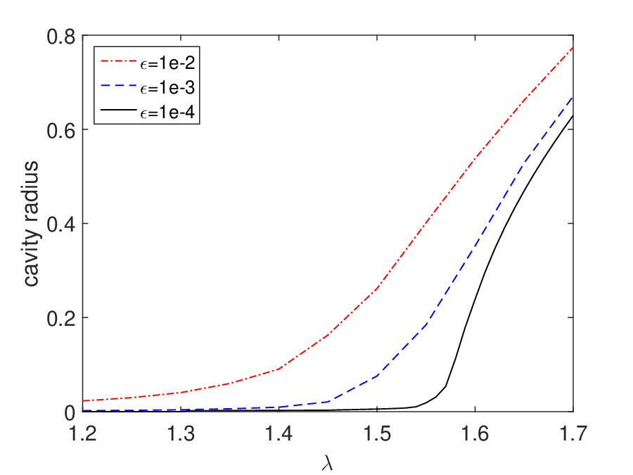
For γ=1\gamma=1 and ε=10−2,10−3,10−4\varepsilon=10^{-2},10^{-3},10^{-4}, we show in Figure 4 the numerical results obtained with M=32M=32 on the λ\lambda-RN​M​(ε)R^{NM}(\varepsilon) (i.e. the expansion rate on the outer boundary against the cavity radius on the inner boundary) graph. Figure 4 shows, for ε=10−4\varepsilon=10^{-4}, the convergence of our numerical results to that of the 1-dimensional ODE solution.

Refer to caption
(a) ε=10−3\varepsilon=10^{-3}, N=16N=16.
Refer to caption
(b) ε=10−4\varepsilon=10^{-4}, N=16N=16.
Figure 2: The convergence behavior of radially-symmetric 𝐔N​M\mathbf{U}^{NM} with N=16N=16 fixed.
Figure 3: λ\lambda-RN​M​(ε)R^{NM}(\varepsilon), N=16N=16, M=32M=32.
Refer to caption
Figure 4: λ\lambda-RN​M​(10−4)R^{NM}(10^{-4}), N=16N=16.
Refer to caption
Refer to caption
(a) radially-symmetric, energy error
Refer to caption
(b) radially-symmetric, cavity radius error
Figure 5: The convergence behavior on Ω(ε,γ)\Omega_{(\varepsilon,\gamma)} with small γ\gamma.

To explore the potential of the method in coupling with a domain decomposition method, especially when combining with a finite element method in a multi-defects problem, we examine the convergence behavior of our algorithm on a small neighbourhood of the defect. Taking Ω(10−3,10−1)\Omega_{(10^{-3},10^{-1})}, Ω(10−4,10−2)\Omega_{(10^{-4},10^{-2})} and Ω(10−5,10−3)\Omega_{(10^{-5},10^{-3})} as the reference configurations and setting λ⋅γ=1.25\lambda\cdot\gamma=1.25, we show in Figure 5 the energy error and cavity radius error as a function of MM (with N=16N=16 fixed), where it is clearly seen that high precision numerical results can be obtained with rather small MM.

5.2 Non-radially Symmetric Case

For the non-radially symmetric case, we consider the circular ring reference configuration Ω(ε,γ)\Omega_{(\varepsilon,\gamma)} with oval boundary stretch 𝐮0​(𝐱)=[λ1​x1,λ2​x2]T\mathbf{u}_{0}(\mathbf{x})=\left[\lambda_{1}x_{1},\lambda_{2}x_{2}\right]^{T}, λ1\lambda_{1}, λ2>1\lambda_{2}>1. Assuming that the error of the numerical solution 𝐔N​M\mathbf{U}^{NM} satisfies

qN​M≈q∞+c1​N−ν1+c2​M−ν2,\displaystyle q^{NM}\approx q^{\infty}+c_{1}N^{-\nu_{1}}+c_{2}M^{-\nu_{2}}, (5.2)

where q∞q^{\infty} and qN​Mq^{NM} represent the exact and numerical results of a specific quantity, such as the elastic energy, semi-major axis and semi-minor axis etc., and c1c_{1}, c2c_{2}, v1v_{1}, v2v_{2} are the corresponding parameters to be determined by the least squares data fitting.

For Ω(ε,γ)=Ω(10−4,1)\Omega_{(\varepsilon,\gamma)}=\Omega_{(10^{-4},1)}, λ1=2.4\lambda_{1}=2.4 and λ2=2\lambda_{2}=2, we show in Figure 6(a) the errors between 𝐔N\mathbf{U}^{N} and 𝐔1.5​N\mathbf{U}^{1.5N} with M=32M=32 fixed, and in Figure 6(b) the errors between 𝐔M\mathbf{U}^{M} and 𝐔1.25​M\mathbf{U}^{1.25M} with N=16N=16 fixed, where Lω2L^{2}_{\omega} and W1,pW^{1,p} represent Lω2​(Ω′)L^{2}_{\omega}(\Omega^{\prime})-norm and W1,p​(Ω(ε,γ))W^{1,p}(\Omega_{(\varepsilon,\gamma)})-semi-norm respectively. The regressed quantities and parameters are shown in Table 2.

Refer to caption
(a) non-radially-symmetric, M=32M=32
Refer to caption
(b) non-radially-symmetric, N=16N=16
Figure 6: The convergence behavior of the non-radially-symmetric 𝐔N​M\mathbf{U}^{NM}.
Table 2: The regressed quantities and parameters for the non-radially-symmetric case.
qq c1c_{1} c2c_{2} ν1\nu_{1} ν2\nu_{2} q∞q^{\infty}
energy 1.45e+24 -3.10e+6 25 6.1 22.85959048
semi-major axis -2.02e+14 -1.37e-1 17 2.1 1.67481624
semi-minor axis -1.61e+14 -8.42e-2 16 2.1 1.42872097

As a comparison, we show in Figure 7 the corresponding errors obtained in the same way for the radially-symmetric case with λ=2\lambda=2, and show in Table 3 the regressed quantities and parameters. It is clearly seen that the regressed formula (5.2) produces quite sharp numerical results in the radially-symmetric case.

Refer to caption
(a) symmetric, ε=10−3\varepsilon=10^{-3}, N=16N=16
Refer to caption
(b) symmetric, ε=10−4\varepsilon=10^{-4}, N=16N=16
Figure 7: The convergence behavior of the radially-symmetric 𝐔N​M\mathbf{U}^{NM}.
Table 3: The regressed quantities and parameters for the radially-symmetric case.
ε\varepsilon qq c2c_{2} ν2\nu_{2} q∞q^{\infty} ODE solution
10−310^{-3} energy -1.38e+8 9.5 18.61960091 18.61960090
cavity radius -3.18e-2 2.0 1.26772534 1.26772534
10−410^{-4} energy -2.22e+6 6.1 18.87582778 18.87582146
cavity radius -1.49e-1 2.1 1.25228561 1.25228643

To see how well the regressed formula (5.2) fits the data, we show in Figure 8(a) the errors on the cavity dimensions, i.e. the cavity radius in the radially-symmetric case and the cavity major and minor axes in the non-radially-symmetric case, and in 8(b) the errors on the elastic energy, between the corresponding quantities produced by the numerical solution 𝐔N​M\mathbf{U}^{NM} and the regressed formula (5.2) respectively. In particular, compare also to Figure 2(b), it is clearly seen that the regressed formula (5.2) is highly accurate and reliable.

Refer to caption
(a) errors on cavity dimensions
Refer to caption
(b) errors on on the elastic energy
Figure 8: Errors on the key quantities produced by 𝐔N​M\mathbf{U}^{NM} and the regressed data.

To examine how the axial ratio of the oval stretch affect the critical displacement, we show in Figure 9 the semi-major and semi-minor axes of the numerical cavity formed as functions of λ1\lambda_{1} for λ1/λ2=1.2,1.3,1.4\lambda_{1}/\lambda_{2}=1.2,1.3,1.4, with Ω(ε,γ)=Ω(10−4,1)\Omega_{(\varepsilon,\gamma)}=\Omega_{(10^{-4},1)}, N=16N=16 and M=32M=32, where it is obviously seen that both are monotonously increasing functions.

Refer to caption
(a) semi-major axis
Refer to caption
(b) semi-minor axis
Figure 9: The semi-major and semi-minor axes of the numerical cavity formed.

Taking Ω(ε,γ)=Ω(10−3,10−1)\Omega_{(\varepsilon,\gamma)}=\Omega_{(10^{-3},10^{-1})}, Ω(10−4,10−2)\Omega_{(10^{-4},10^{-2})}, Ω(10−5,10−3)\Omega_{(10^{-5},10^{-3})} as the reference configuration respectively, setting the oval boundary data λ1​γ=1.67\lambda_{1}\gamma=1.67 and λ2​γ=1.42\lambda_{2}\gamma=1.42 (see Table 2), for N=16N=16 fixed, the errors of the corresponding non-radially-symmetric numerical solutions 𝐔N​M\mathbf{U}^{NM} are shown in with Figure 10, where the numerical solution with M=32M=32 is taken as the exact solution. It is clearly seen that high precision numerical results can also be obtained in a neighborhood of a defect with rather small MM in non-radially-symmetric case.

Refer to caption
(a) non-radially-symmetric, energy error
Refer to caption
(b) semi-major axis error
Figure 10: The convergence behavior on Ω(ε,γ)\Omega_{(\varepsilon,\gamma)} with small γ\gamma.

References

  • [1] Gent, A. N. and Lindley, P. B. Internal rupture of bonded rubber cylinders in tension. Proceedings of the Royal Society. Series A, 249, 195–205 (1958)
  • [2] Gent, A. N. and Park, B. Failure processes in elastomers at or near a rigid spherical inclusion. Journal of Materials Science, 19, 1947–1956 (1984)
  • [3] Lazzeri, A. and Bucknall, C. B. Dilatational bands in rubber-toughened polymers. Jounal of Materials Science, 28, 6799–6808 (1993)
  • [4] Bucknall, C. B., Karpodinis, A. and Zhang, X. A model for particle cavitation in rubber toughened plastics. Journal of Materials Science, 29, 3377–3383 (1994)
  • [5] Ball, J. M. Discontinuous equilibrium solutions and cavitation in nonlinear elasticity. Philosophical Transactions of the Royal Society of London. Series A, Mathematical and Physical Sciences, 306, 557–611 (1982)
  • [6] Sivaloganathan, J. and Spector, S. J. On cavitation, configurational forces and implications for fracture in a nonlinearly elastic material. Journal of Elasticity, 67, 25–49 (2002)
  • [7] Sivaloganathan, J., Spector, S. J. and Tilakraj, V. The convergence of regularized minimizers for cavitation problems in nonlinear elasticity. Siam Journal on Applied Mathematics, 66, 736–757 (2006)
  • [8] Henao, D. Cavitation, invertibility, and convergence of regularized minimizers in nonlinear elasticity. Journal of Elasticity, 94, 55–68 (2009)
  • [9] Lavrentiev, M. Sur quelques problèmes du calcul des variations. Annali di Matematica Pura ed Applicata, 4, 7–28 (1927)
  • [10] Xu, X. and Henao, D. An efficient numerical method for cavitation in nonlinear elasticity. Mathematical Models and Methods in Applied Sciences, 21, 1733–1760 (2011)
  • [11] Lian, Y. and Li, Z. A dual-parametric finite element method for cavitation in nonlinear elasticity. Journal of Computational and Applied Mathematics, 236, 834–842 (2011)
  • [12] Lian, Y. and Li, Z. A numerical study on cavitations in nonlinear elasticity-defects and configurational forces. Mathematical Models and Methods in Applied Sciences, 21, 2551–2574 (2011)
  • [13] Su, C. and Li, Z. Error analysis of a dual-parametric bi-quadratic FEM in cavitation computation in elasticity. Siam Journal on Numerical Analysis, 53, 1629–1649 (2015)
  • [14] Negrón-Marrero, P. V. and Betancourt, O. The numerical computation of sigular minimizers in two-dimensional elasticity. Journal of Computational Physics, 113, 291–303 (1994)
  • [15] Celada, P. and Perrotta, S. Polyconvex energies and cavitation. Nonlinear Differential Equations and Applications, 20, 295–321 (2013)
  • [16] Li, J. and Guo, B. Fourier-Chebyshev pseudospectral method for three-dimensional Navier-Stokes equations. Japan Journal of Industrial and Applied Mathematics, 14, 329–356 (1997)
  • [17] Shen, J. A new fast Chebyshev-Fourier algorithm for Poisson-type equations in polar geometries. Applied Numerical Mathematics, 33, 183–190 (2000)
  • [18] Shen, J., Tang, T. and Wang, L. Spectral Methods: Algorithms, Analysis and Applications, Springer, Heidelberg, 154–157 (2011)
  • [19] Gottlieb, S., Jung, J. H. and Kim, S. A review of David Gottlieb¡¯s work on the resolution of the Gibbs phenomenon. Communications in Computational Physics, 9, 497–519 (2011)
  • [20] Nocedal, J. and Wright, S. J. Numerical Optimization, Springer, New York, 31-45 (1999)
  • [21] Su, C. The Numerical Analysis of Iso-parametric and Dual-parametric Finite Element Methods Applied in Cavitation (in Chinese), Ph. D. dissertation, Peking University, 73–74 (2015)
  • [22] Morrey, C. B. Poincaré inequality. Multiple Integrals in The Calculus of Variations, Springer, New York (1966)
  • [23] Meyer, P. A. De La Vallée Poussin theorem. Probability and potentials, Blaisdell Publishing Company, London (1966)
  • [24] Henao, D. and Mora-Corral, C. Fracture surfaces and the regularity of inverses for bv deformations. Archive for Rational Mechanics and Analysis, 201, 575–629 (2011)
  • [25] Henao, D. and Mora-Corral, C. Invertibility and weak continuity of the determinant for the modelling of cavitation and fracture in nonlinear elasticity. Archive for Rational Mechanics and Analysis, 197, 619–655 (2010)
  • [26] Ball, J. M., Currie, J. C. and Olver, P. J. Null Lagrangians, weak continuity, and variational problems of arbitary order. Journal of Functional Analysis, 41, 135–174 (1981)
  • [27] Adams, R. A. Sobolev Spaces, Academic Press, New York, 40–45 (1975)
  • [28] Brezis, H. Analyse Fonctionnelle: Théorie et Applications, Masson, Paris, 53–54 (1983)
  • [29] Sivaloganathan, J. The numerical computation of the critical boundary displacement for radial cavitation. Mathematics and Mechanics of Solids, 14, 696–726 (2009)