Phase Space Sketching for Crystal Image Analysis
based
on Synchrosqueezed TransformsThanks: J.L. was supported in part by the National Science Foundation under awards DMS-1454939 and ACI-1450372. H.Y. thanks the support of the startup grant from National University of Singapore. We would like to thank Yilong Han and Yang Xiang for helpful discussions.
Abstract.
Recent developments of imaging techniques enable researchers to visualize materials at the atomic resolution to better understand the microscopic structures of materials. This paper aims at automatic and quantitative characterization of potentially complicated microscopic crystal images, providing feedback to tweak theories and improve synthesis in materials science. As such, an efficient phase-space sketching method is proposed to encode microscopic crystal images in a translation, rotation, illumination, and scale invariant representation, which is also stable with respect to small deformations. Based on the phase-space sketching, we generalize our previous analysis framework for crystal images with simple structures to those with complicated geometry.
Key words and phrases:
Atomic resolution crystal image, phase-space sketching, D synchrosqueezed transform, transformation invariance, texture classification, image segmentation.2000 Mathematics Subject Classification
65T99,74B20,74E15,74E251. Introduction
Crystal image analysis at the atomic resolution has become an important research direction in materials science recently [1, 26, 3, 36, 14]. The advancement of image acquisition techniques enable researchers to visualize materials at atomic resolution, with images of clearly visible individual atoms and their types (see Figure 1 (a)) and defects such as dislocations and grain boundaries (see Figure 1 (f)). These high-resolution images provide unprecedented opportunities to characterize and study the structure of materials at the microscopic level, which is crucial for designing new materials with functional properties.
The recognition of important quantities and active mechanisms (e.g., dislocations, grain boundaries, grain orientation, deformation, cracks) in a material requires the use of automatic and quantitative analysis by computers. Due to the extraordinarily large volume of measurements and simulations in daily research activities (see Figure 1), in particular, in the case of analyzing a time series of crystal images during the dynamic evolution of crystallization [22], crystal melting [19, 21], solid-solid phase transition [20], and self-assembly [6] etc., it is impractical to analyze these images manually. In the case of crystal images with complicated geometry (see Figure 1 (b) for an example), it becomes difficult to recognize and parametrize the image patterns by visual inspection. Moreover, it is also difficult, if not impossible, to measure crystal deformation directly from crystal images by hand. Therefore, there is a dire need for efficient tools to classify and analyze atomic resolution crystal images automatically and quantitatively, with minimal human intervention.
 |
 |
 |
| (a) | (b) | (c) |
 |
 |
 |
| (d) | (e) | (f) |
There have been several types of methods for atomic resolution crystal image analysis, assuming simple crystal patterns are known a priori, typically a hexagonal or a square reference lattice in two dimensions (see Figure 2). One class of methods tries to estimate atom positions first (or assume knowledge of the atom positions), and then compute the local lattice orientation and deformation as well as defects via identifying the nearest neighbors of each atom [27]. Other methods are based on a local, direction sensitive frequency analysis, e.g. wavelets [24] to segment the crystal image into several crystal grains and identify their orientations. Another more advanced class of methods formulates the crystal analysis problem (such as segmentation) as an optimization problem with fidelity term specially designed for the local periodic structure of the crystal image [1, 26, 3, 17].
Existing methods however often fall short for crystal image analysis with a variety of crystal patterns, fine features, and complicated geometry (see Figure 1 for examples). For instance, when the out-of-focus problem occurs, usually in optical microscopies and bright-field microscopies, the image intensity at the centers of atoms might vary a lot over the imaging domain, making it difficult to determine the reference configuration for atoms (see Figure 3 (left) for an example).
In this paper, we propose a two step procedure for crystal image analysis in these challenging scenarios. In the first step, an efficient phase-space sketching method is used to classify complicated crystal configurations and determine reference crystal patterns. In the second step, once the reference crystal patterns are learned from the first step, a recently developed crystal image analysis method based on two-dimensional synchrosqueezed transforms [36, 14] is applied to identify dislocations, cracks, grain boundaries, crystal orientation, deformation, and possibly other useful information.
 |
 |
A major difficulty of crystal pattern classification comes from the considerable variability within object classes and the inability of existing distances to measure image similarities. Part of this variability is due to grain orientation, crystal deformation, and defects; another part results from the imaging variation, e.g., the difference of image illumination, light reflection, and out-of-focus issues. An ideal transformation for classification should provide a representation invariant to such uninformative variability. Note that a representation that is completely invariant with respect to deformation would not distinguish different Bravais lattices (see Figure 2), since the lattices are equivalent up to affine transforms. The crystal image representation must therefore be capable of distinguishing different lattices, while being invariant to small elastic deformation due to external forces on grains.
Texture classification has been extensively studied in the literature. Translation and rotation invariant representations have been standard tools: these representations can be constructed with autoregression methods [9], hidden Markov models [30], local binary patterns [4], Gabor or wavelet transform modulus with rotation invariant features [5]. Scale and affine invariance has been also studied recently using affine adaption [12], fractal analysis [32], advanced learning [29], and combination of filters [39]. More recently, deep convolution networks [15] together with advanced learning techniques [2] have been applied to design deformation invariant representations [23]. Combined with advanced learning techniques, the convolution neural network (CNN) and the scattering transform can provide deformation invariance and could be used for the problem discussed in this paper. To achieve transformation invariance using deep learning, most current methods usually make use of dataset augmentation; but this requires larger number of model parameters and training data, because the learned model needs to capture enough features for all the possible transformations of the input. Hence, methods in this direction is very expensive. A recent work [11] combines the pooling idea and deep CNN to achieve transformation invariance while keeping the computational expense relatively low. However, all crystal lattices are equivalent up to an affine transformation (see Figure 2 for examples) and we only need the invariance to crystal elastic deformation that is relatively much smaller than the affine transformation. How to tune the extend of deformation invariance via the method in [11] to match the demand in crystal image analysis is still worth to explore. On the other hand, since our problem is more specific than general image classification, we aim to design a more efficient and specific method, taking advantage of the periodic structure of crystal images. The proposed phase-space sketching is a nonlinear operator that rescales, shifts, and coarsens (i.e., pooling) the synchrosqueezed (SS) energy distribution. Since the SS energy distribution has already been computed for the analysis of crystal orientation, defects, and deformation, the computational cost of which scales nearly linearly in terms of the image size (see [36]), the additional computational cost for the phase-space sketch is almost negligible, since we just need to sum up the synchrosqueezed representation using a coarser grid, which scales linearly in the size of the phase-space representation by the synchrosqueezed transform.
The phase-space sketching proposed in this paper is an alternative method for the invariant texture classification based on the two-dimensional synchrosqueezed transform [37, 38]. The phase-space sketching encodes microscopic crystal images in a translation, rotation, illumination, and scale invariant representation. This new representation is stable to deformation and invariant to a class of elastic deformation in materials. The extent of the elastic deformation invariance is specified by user-defined parameters. As we shall see later, the results of the two-dimensional synchrosqueezed transforms can be applied to identify dislocations, cracks, grain boundaries, crystal orientation and deformation following the algorithms in [36, 14]. The proposed phase-space sketching only adds minimal computational cost to our existing methodologies for atomic resolution crystal image analysis. We remark that it is also possible to extend existing approaches of texture segmentation methods combined with classification procedure to achieve our goal of crystal image analysis of complex geometry in this paper, the advantage of the proposed method is to put all these image analysis steps in a single framework based on synchrosqueezed transforms, which have been shown to be suitable for crystal image analysis.
The rest of this paper is organized as follows. We start by introducing the mathematical model of atomic resolution crystal images and our previous analysis framework on crystal image analysis in Section 2. In Section 3, we propose the phase space sketching based on the two-dimensional synchrosqueezed transform to identify reference crystal patterns. With the reference crystal patterns ready, a complete algorithm for invariant texture classification and segmentation is introduced. We apply the whole algorithm to several real examples in materials science in Section 4. Finally, we present a brief summary of the proposed methodology in Section 5.
2. Crystal image modeling and synchrosqueezed transform (SST)
2.1. Mathematical models for atomic resolution crystal image
Consider an atomic resolution image (experimentally, this is often done for a thin slice of a polycrystalline material) that may consist of multiple grains with the same Braivas lattice. Denote the reference Bravais lattice as
where represent two fixed linearly independent lattice vectors (see Figure 2 for examples). Let be the shape function describing a single perfect unit cell in the image, extended periodically in with respect to the reference crystal lattice. We denote by an open set , , the grains the system consists of, and by the domain occupied by all grains. We only consider disjoint sets in this paper. In more complicated cases when there are overlapping grains, it would be interesting to extend the mode decomposition techniques for one-dimensional oscillatory signals in [31, 33] to two-dimensional so as to decompose overlapping grains. Hence, not considering grain boundaries, the polycrystal image can be modeled as
| (1) |
where is the reciprocal lattice parameter (or rather the relative reciprocal lattice parameter since the dimension of the image is normalized in our analysis). The crystal image model above works for both simple lattices (Braivais lattices listed in Figure 2) and complex lattices (such that the unit cell consists more than one atoms); extensions to more complicated images will be considered below. Here is the indicator function of each grain ; maps the atoms of grain back to the configuration of a perfect crystal, i.e., it can be understood as the inverse of the elastic deformation. The local inverse deformation gradient is then given by in each . The smooth amplitude envelope and the smooth trend function in (1) model possible variation of intensity, illumination, etc. during the imaging process. By the Fourier series of , we can rewrite (1) as
| (2) |
where is the reciprocal lattice of (recall that the shape function is periodic with respect to the lattice ).
 |
 |
 |
 |
| (a) | (b) | (c) |
 |
 |
 |
| (d) | (e) | (f) |
 |
 |
 |
 |
 |
 |
 |
2.2. Synchrosqueezed transform (SST)
As shown in [36, 14], the 2D SST is an efficient tool to estimate the defect region and also the local inverse deformation gradient in the interior of each grain . The main observation is that, in each grain , the image is a superposition of planewave11 1 Planewave is a wave with constant frequency or wave vector.-like components with local wave vectors . It has been shown in [37, 38] that the SST is able to estimate the local wave vectors accurately. Based on the local wave vector estimation, we can compute the inverse deformation gradient via a least square method, see §2.3 below.
The starting point of D SST is a wave packet , which is, roughly speaking, constructed by translating, rotating, and rescaling or modulating a mother wave packet according to the spatial center parameter , the angular parameter in the frequency domain, and the radial parameter in the frequency domain [37, 38, 36, 14]. To introduce the definition of wave packets, let us define the following notations:
- (1)
The scaling matrix
where is the distance from the center of one wave packet to the origin in the Fourier domain.
- (2)
A unit vector with a rotation angle .
- (3)
represents the argument of a given vector .
- (4)
of denotes a mother wave packet, which is in the Schwartz class and has a non-negative, radial, real-valued, smooth Fourier transform with a support equal to a ball centered at the origin with a radius in the Fourier domain. The mother wave packet is required to obey the admissibility condition: such that
for any .
Definition 1.
For , define as a wave packet in the Fourier domain. Equivalently, in the space domain, the corresponding wave packet is
In such a way, a family of wave packets is constructed.
Definition 2.
The wave packet transform22 2 Throughout this paper all the numerical implementation of integration follows the rectangle rule. For the purpose of simplicity, we don’t specify the discretization of all variables in this paper. In a general setting, we assume the given image of size is defined on with grid points for ; the frequency domain in a Cartesian coordinate is discretized with grid points for ; unless specified, the frequency domain in a polar coordinate is restricted in the range or for radius and for angle, and they are discretized uniformly with step size in radius and in angle. The code for phase-space sketching and the test data are available online in the SynCrystal package for reference (https://github.com/SynCrystal/SynCrystal). of a function is a function
for , , . For convenience, we also set for .
More specifically, the discrete wave packets are constructed via the partition of unity in the frequency domain (see Figure 4) so that they have compact supports in the frequency domain. The Fourier transform of a wave packet is essentially the product of a bump function and a plane wave. Figure 4 (left) illustrates the positions of the centers of bump functions and Figure 4 (right) shows an example of a bump function when its center has a radius . The reader is refered to Section of [38] for detailed implementation of the discret wave packet transform. As shown in Figure 4 (right), there are two scaling parameters to control the geometry of the supports of wave packets. If , the wave packet transform is essentially the wavelet transform; if , the wave packet transform becomes the curvelet transform (see Figure 3 (right) for an illustration). The wave packet transform is a generalization of curvelet and wavelet transforms with better flexibility in frequency scaling and consequently is better suited to analyze crystal images with complicated geometry. As a convolution with smooth wave packets, is well-defined and smooth even under very low regularity requirements for , e. g. .
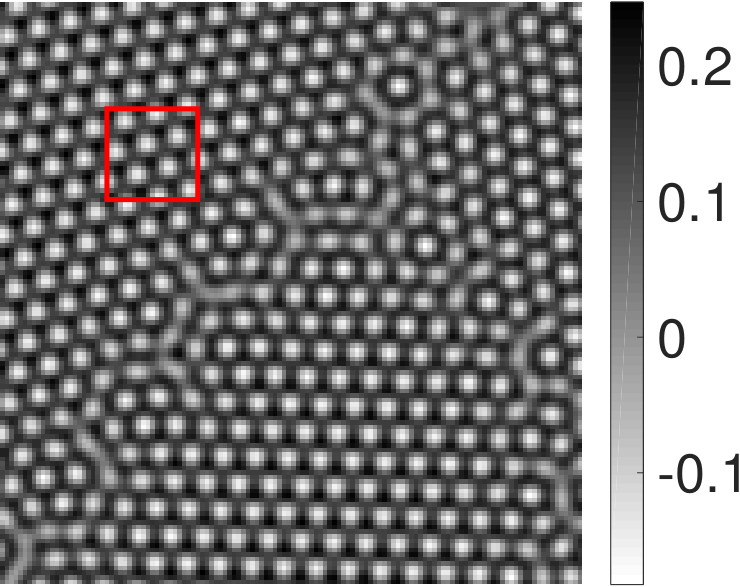
In contrast to the windowed Fourier transform of a given crystal image, whose spectrum spreads out in the phase space as illustrated in Figure 5(b), the D synchrosqueezed transform (SST) based on wave packets aims at a sharpened phase-space representation. In the SST, for each , we define the corresponding local wave vector estimation
| (3) |
for , where is a threshold parameter to ensure stability of the estimation. Here, denotes the gradient of with respect to its third argument .
If is a plane wave with a wave vector , then simple algebraic calculation shows that the local wave vector estimation is exactly whenever is not zero. When is a superposition of planewaves with well-separated local wave vectors , by the stationary phase approximation, when is close to some local wave vector . In the case of crystal images, locally is a superposition of deformed planewaves. By applying Taylor expansion to make approximations, one can also show that the local wave vector estimation can still approximate the local wave vectors of . Even in the presence of heavy noise, this approximation is still reasonably good by applying the SST based on highly redundant wave packet frames [34, 35]. More precisely, let us revisit the theory developed in [36] to support the argument just above.
Definition 3 ( general shape function).
The general shape function class consists of periodic functions with a periodicity , a unit -norm, and an -norm bounded by satisfying the following conditions:
- (1)
The Fourier series of is uniformly convergent;
- (2)
and ;
- (3)
Let be the set of integers . The greatest common divisor of all the elements in is .
Definition 4 ( general intrinsic mode type function (GIMT)).
A function is a GIMT of type , if , and satisfy the conditions below.
The theorem below shows that the local wave vector estimation precisely estimates the local wave vectors of the crystal image at the points away from boundaries (see [36] for the proof).
Theorem 5.
For a GIMT of type with any and any , we let and define
and
For fixed , , , , , and , there exists such that for any and a GIMT of type , the following statements hold.
- (1)
are disjoint and ;
- (2)
For any ,
For simplicity, the notations , and are used when the implicit constants may only depend on , , , and .
Motivated by the property of the local wave vector estimation , the synchrosqueezed (SS) energy distribution of is constructed as
| (4) |
where
and in (4) denotes the Dirac measure. In the numerical implementation of in (4), a normalized Gaussian function with a sufficiently small support (of the same order as the discretization step size of its domain) is applied to approximate the Dirac delta function. The discretization of and is given by the partition of unity of the discrete wave packet transform. The variable is discretized uniformly in the Cartesian coordinate, while the variable is discretized in the polar coordinate. The SST squeezes the wave packet spectrum according to to obtain a sharpened and concentrated representation of the image in the phase space. Hence, in the interior of a grain, the SS energy distribution has a support concentrating around local wave vectors , , and is given approximately by (see e.g., Figure 5(c) in polar coordinate)
| (5) |
understood in the distributional sense. Therefore, by locating the energy peaks of , we can obtain estimates of local wave vectors and also their associated spectral energy. In practice, we choose high energy peaks corresponding to close to the origin in the reciprocal lattice to estimate the inverse deformation gradient and grain boundaries to guarantee numerical stability.
2.3. SST based crystal image analysis
In the case of a crystal image that consists of only one kind of lattice in the image, it has been shown in [36, 14] that the SST can be applied to estimate the inverse deformation gradient , grain boundaries, and defects. For simplicity, let us focus on the case of hexagonal lattices in this section. It is straightforward to generalize to other Bravais lattices.
In the case of hexagonal lattices, we have six dominant reciprocal lattice vectors such that is significant, which can be further reduced to three due to the symmetry . We will henceforth denote these as , , and denote by the estimate of . The inverse deformation gradient is determined by a least squares fitting to identify a linear transformation that maps the reference reciprocal lattice vectors to the estimated local wave vectors :
In practice, for each physical point we represent in polar coordinates (the information in is redundant due to symmetry). To identify the peak locations , we choose the grid point with highest amplitude in each -degree sector of .
Since the local wave vector estimation is no longer valid around the crystal defects, the SS energy distribution does not have dominant energy peaks around local wave vectors. Hence, we may characterize the defect region by quantifying how concentrated the energy distribution is. One possible way is to use an indicator function as follows. For each (corresponding to one of the sectors), we define
where denotes a small ball around the estimated local wave vector , and means the argument of . Hence, will be close to in the interior of a grain due to (5), while its value will be much smaller than near the defects. This is illustrated in Figure 5(e), where we show for the crystal image in Figure 5(a). The estimate of defect regions can be obtained by a thresholding at some value according to
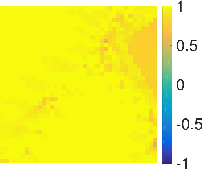
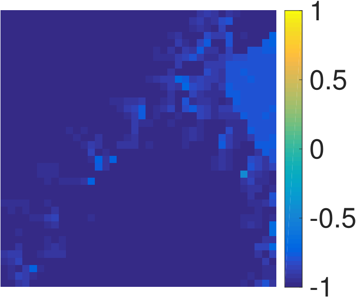
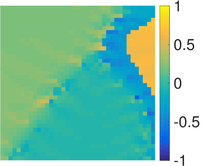
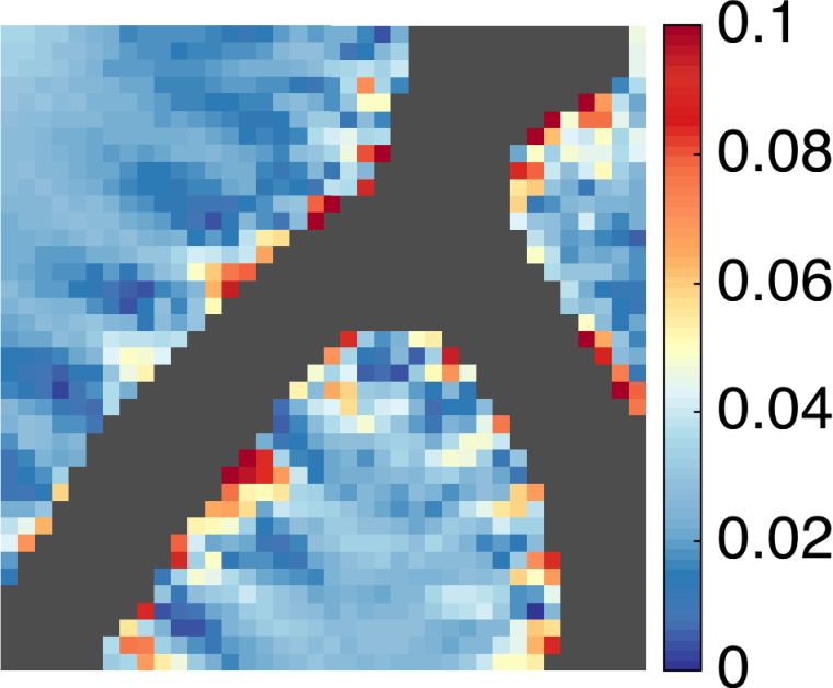
an illustration of which is shown in Figure 5(f). Figure 6 shows the estimate of by the SST. When showing the result, we have used a more transparent way to represent the inverse deformation gradient via the polar decomposition for each point , where is a rotation matrix and is a positive-semidefinite symmetric matrix. At each position , the crystal orientation can be estimated via the rotation angle of ; the volume distortion of can be visualized by ; the quantity characterizes the difference in the principal stretches of as a measure of shear strength, where and are the eigenvalues of . The bottom panel of Figure 6 shows these quantities corresponding to the estimate of in the top panel. In later numerical examples, we will always present the estimated inverse deformation gradient in the same fashion.
3. Phase space sketching
To extend the crystal image analysis to more complicated scenario, in this section, we propose the phase-space sketching, which is a sparse invariant representation of the phase-space information obtained by synchrosqueezed transforms. The phase-space sketching will enable classification of different crystal types presented in the same image or across images.
3.1. Invariant representation
As compared to the crystal image model with a unique Bravais lattice in the previous section, the mathematical model of a crystal image that consists of multiple types of lattices can be written as in (1) and (2).
The image classification and segmentation problem is to identify each domain and classify its corresponding shape function . The main difficulty is due to the considerable variability within object classes (e.g., grain orientation, crystal deformation, defects, and difference of image illumination). Our goal is to design a representation of the crystal image that is invariant to most of these variability.
It has been shown in [13, 2] that, deep convolution networks have the ability to build large-scale invariants stable to deformations. Combined with advanced learning techniques, the convolution network like the scattering transform can provide deformation invariance [23] and could be used for the problem discussed in this paper. On the other hand, since our problem is more specific than general image classification, we aim to design a more efficient and specific method. Taking advantage of the periodic structure of crystal images, we introduce the phase-space sketching instead of applying the convolution network for the purpose of computational efficiency. The phase-space sketching is a nonlinear operator rescaling, shifting, and coarsening the SS energy distribution.
 |
 |
 |
Let us recall the definition of the SS energy distribution in Equation (4), written in polar coordinate as
| (6) |
for . Note that the SS energy distribution is translation invariant because the modulus of the wave packet coefficient is invariant to the translation of the image . A simple idea to achieve the rotation invariance might be shifting in the variable such that always takes its maximum value at a specific location. However, this shifting procedure is usually sensitive to the crystal deformation. This motivates the following shifting and coarsening process to reduce the influence of rotation and deformation simultaneously. For a step size in the angle coordinate and a step size in the radial coordinate , we define the phase-space sketch via a coarsening procedure as follows.
Let
we defined the shifted and rescaled SS energy distribution with a scaling parameter as
| (7) |
In the maximization above, we approximate with a finite set of points, numerically evaluate the objective at all these points, and identify the maximizer by simply traversing all the points. To reduce the computational cost for traversing, we will project the matrix in and into 1D vectors in and look for the peaks in first. Once the peaks in have been identified, it is only necessary to search for peaks in for around the peaks in . This can reduce the computational complexity to a linear scaling one in terms of the number of grid points in and . Typical choices are or grid points in both angle and radius domains for all numerical examples in this paper. Hence, the total computational cost for all is in the order of times the number of pixels. The step size is usually chosen to be or , and the step size is usually chosen to be or of the lowest frequency of wave-like components in the crystal image, i.e., in our mathematical model in Equation (2), which can be estimated by the SST by Theorem 5. The same parameters will be used to discretize the angle and radius domain, and to do the sketching for other formulas in this paper since the proposed method is not sensitive to them. For a fixed , there might be multiple maximizer but one can simply choose one of them. is not sensitive to the choice of due to the concentration of the phase space representation and the largest spectrum energy of crystal images is assocated with the energy bump with the lowest wave number. Then the phase-space sketch of the new SS energy distribution is defined as a local average of the shifted and rescaled SS energy distribution
| (8) |
for , where means the floor operator.
This operation can be understood as a binning (or pooling) operator that collects varying local wave vectors into fixed bins in the phase space, and hence reduces the influence of the deformation. Overall, the phase-space sketching is a nonlinear transform (with respect to the image ) that squeezes the phase-space energy distribution via synchrosqueezing and coarsening into the sketch , resulting in a representation invariant to small deformation.
The extend of the deformation invariance of is determined by the step sizes and . Note that a fully deformation invariant representation would not be able to distinguish different Bravais lattices (see Figure 2), since these lattices are the same in the quotient group of affine transforms. Hence, we should choose appropriate step sizes and such that: 1) they are sufficiently large, making invariant to small elastic deformation due to external forces on the material; 2) they are small enough such that is capable of distinguishing different lattices.
The sketch is also invariant to rotation and scaling. After shifting and rescaling, for a fixed , the new SS energy distribution reaches its maximum value at . Hence, the sketch has the maximum value in for each fixed .
It is worth pointing out that the sketch is separably invariant with respect to rotation and translation. Therefore, the sketch cannot discriminate a class of similar texture patterns, e.g. see Figure 8 for an example of two images sharing similar absolute values of the wave packet coefficients. Fortunately, this is not a problem in atomic resolution crystal image analysis, since all crystal patterns behave similarly to the pattern in Figure 8 (left).
Finally, to remove the influence of the amplitude function , i.e., obtaining the illumination invariance, we normalize the magnitude of the phase-space sketch and define
| (9) |
 |
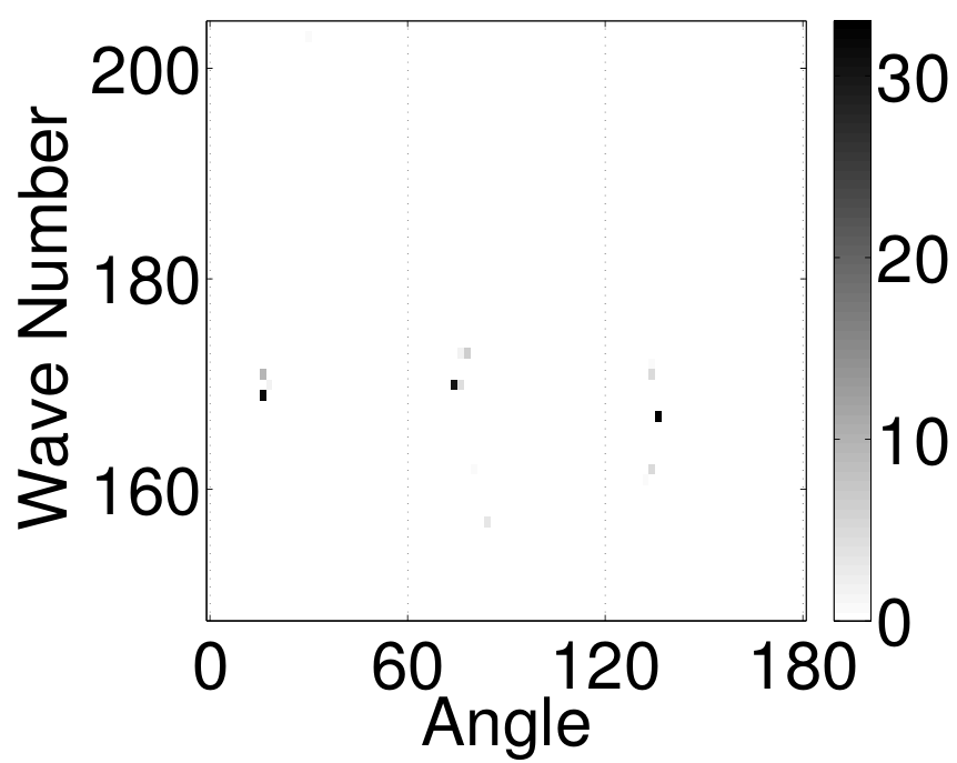
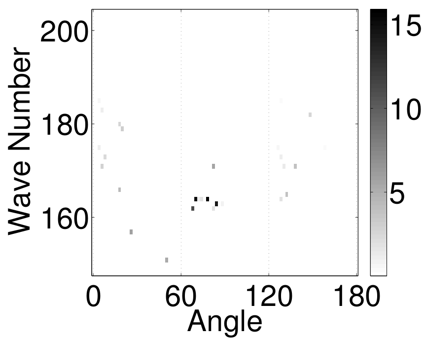
One may also consider sketching other more standard phase-space representations, e.g., the polar windowed Fourier transform or wavelet transform. However, it is more advantageous to combine sketching with the synchrosqueezed transforms. As we have shown in Figure 5, the SS energy distribution has concentrated support around the local wave vectors of the crystal image, while the results of windowed Fourier transform or wavelet transform are more spread-out. Hence, the sketch of the windowed Fourier or wavelet transform is not as clean as that of the SS energy distribution (see the comparison in Figure 7). Moreover, the SS energy distribution provides useful information for crystal image analysis and computing its sketching only adds minimal computational overhead.
Finally, we close the introduction of phase space sketching with the following theorem.
Theorem 6.
Suppose and for are two GIMT’s of type and , respectively, such that is a shape function describing one crystal configuration (square or hexegonal lattice). and , let , compute the local wave vector estimations as in (3) and the SS energy distribution as in (6) in the domain for and . given by Theorem 5 such that , , and , if positive numbers , , and satisfy the following conditions:
where , , then the phase space sketch of and satisfy
for all .
Proof.
The proof of Theorem 6 is straightforwad and only need elementary algebraic calculation. The intuition is that when is sufficiently large, we have thresholded less important features in the shape function and only a few important local wave vectors of crystal images are left for pooling, which allows the choices of , , and such that the phase space sketch only contains a few nonzero energy bins indicating the type of crystal configuration. We will focus on the case of square lattice and use Figure 9 to sketch out the proof. Let’s assume without the loss of generality since we can rescale the SS energy distribution according to (7). Orange areas in Figure 9 (a) and (b) denote the supports of the SS energy distribution for some vector and for a fixed ; the green areas denote the supports of for the same and ; the blue areas cover the possible supports of for all with the fixed . By Theorem 5, we can estimate the size of these colored areas up to a constant prefactor independent of (see quantitative estimations in Figure 9 (b)). Hence, after shifting and rescaling, we obtain in Figure 9 (c) and in Figure 9 (d). Finally, as long as and are large enough such that the blue areas in Figure 9 (c) and (d) are covered in a box given by the grids, then we see that the phase space sketches of and are the same up to in the range . The conditions , and make sure that a single bin in the phase space sketches can cover one blue area in Figure 9 (c) and (d). ∎
Theorem 6 shows that for crystal images with the same type of configuration (either square or hexagonal lattice), their phase space sketches are invariant to image translation, rotation, illumina- tion, and scale difference. This new representation is also stable to deformation and invariant to a class of elastic deformation characterized by the phase function in 2D GIMTs. When the parameter in a GIMT is , it is easy to find parameters , , and to construct the phase space sketch. However, if is large, there is no good parameter to obtain invariant representations via phase space sketching.
 |
3.2. Classification
We may apply the phase-space sketch to classify crystal textures in a complicated crystal image. Although advanced classifiers such as SVM are useful tools for classification, here we present some simple and efficient classification methods.
As we have seen in Figure 7, the phase-space sketch at a point in the interior of a grain has well-separated supports indicating the reciprocal lattice of the Bravais lattice of the crystal pattern. Hence, the locations and the magnitudes of the supports are important features for crystal pattern classification. In the case of a complicated crystal image, if two grains share the same crystal pattern, they should have the same phase-space sketch at the locations sufficiently far away from grain boundaries. Therefore, we only need to identify major groups of the sketch at different ’s and choose a representative sketch from each major group. Other sketch outliers are due to the influence of grain boundaries on the phase-space representation; each sketch outlier contains the information of at least two crystal patterns and looks like a superposition of more than one sketches.
 |
 |
A simple idea for classification is to define an appropriate distance to measure the similarity of different phase-space sketches and apply the spectral clustering [18] to identify the major groups of the sketches. Since the types of crystal textures are limited, it is not necessary to use the whole sketch for discrimination. To ensure that the method is as efficient as possible, features contained in the sketch invariant to uninformative variability in crystal images are more important. Observe that the phase-space sketch is able to sketch out the multi-scale reciprocal lattice (see Figure 7 (right)), and the numbers of supports at different scales largely determine the crystal pattern. It is sufficient to use these numbers as a compressed feature vector to represent the sketch. For example, the feature vector of the sketch in Figure 7 (right) is , where each means that there are leading supports above a certain threshold at each scale (each row in the phase space sketch matrix). For some other examples for the feature vectors, please see Figure 11. Note that the number of supports are invariant to translation, rotation, illumination, and small deformation. Hence, the feature vector by the number of supports in sketches is a compressed invariant representation of crystal patterns. The standard Euclidean distance of vectors is a natural choice to measure the similarity of these compressed invariant representations. Using the number of supports only might be too ambitious in some cases. A better way is to take advantage of the magnitudes of the peaks in these supports, once two crystal patterns have sketches sharing the same numbers of supports. For example, a simple idea is to set up a threshold parameter and only count the number of supports above this threshold. In practice, this simple idea is sufficient to discriminate most crystal patterns in real applications.
 |
 |
 |
 |
| Type | Type | Type | Type |
Finally, we provide several synthetic examples to demonstrate the efficiency of the proposed compressed feature vector for classification. The first example in Figure 10 (left) contains three different crystal patterns and one vacancy area, and each pattern has two grains with different orientations and scales. The SST is applied to generate the phase-space sketch and the corresponding compressed feature vectors at each pixel of the crystal image. The spectral clustering algorithm is able to identify four major groups of compressed feature vectors. According to the clustering results of the feature vectors, we group the corresponding pixels together and visualize the results in Figure 11 (right).
 |
 |
 |
 |
 |
 |
| Type | Type | Type | Type |
The third example in Figure 12 (left) is similar to the first example but the crystal image has been smoothly deformed. As shown in Figure 12 (right) and Figure 13, the proposed method succeeds to detect all crystal patterns and their sketches.
In the last example in Figure 14 (left), there are four different crystal patterns (two kinds of square lattices and two kinds of hexagonal lattices) with different levels of illumination. As shown in Figure 14 (right) and Figure 15, the proposed method is able to detect all crystal patterns and their sketches. This is a very challenging example. As we can see in the sketches in Figure 15, Type and sketches almost share the same support (and so do Type and ). Hence, as discussed previously, only the number of supports with peaks over an appropriate threshold is used in constructing the compressed feature vector.
 |
 |
 |
 |
 |
 |
| Type | Type | Type | Type |
To demonstrate the efficiency of the phace-space sketching method, we quantitatively compare it with the state-of-the-art algorithms33 3 In our numerical tests, CNN [15] doesn’t perform well because crystal image data are limited and it is difficult to regularize the CNN with sufficiently good data augmentation. Hence, we only compare our algorithm with the scattering transform. Default parameters were used in the scatterign transform., e.g. the scattering transform in [23], using the examples in Figure 12 and 14. Each example contains four different kinds of crystal texture; correspondingly, training images of size by with different orientation, translation, image intensity, deformation were generated for each texture class. Crystal images on the left of Figure 12 and 14 were partitioned into overlapping patches of size uniformly distributed in the image domain and these patches are used as validation data. The scattering transform was used to train and classify these data. Table 1 and 2 summarize the performance of the propose method and the scattering transform. Numerical results show that the phase space method is highly efficient in running time and the success rate is higher than the scattering transform. The code and the data set for this comparison are available in the SynCrystal package. The numerical tests were performed on a MacBook Pro (processor 3.1 GHz Intel Core i5, memory 8 GB 2133 MHz LPDDR3).
| Example | Algorithm | Success Rate | ||
|---|---|---|---|---|
| Figure 12 | non-log | 8.65e+02 | 2.60e-02 | 84.6 |
| Figure 12 | log | 8.80e+02 | 3.02e-02 | 88.3 |
| Figure 14 | non-log | 8.78e+02 | 2.60e-02 | 82.0 |
| Figure 14 | log | 8.95e+02 | 2.60e-02 | 82.8 |
| Example | Success Rate | |||
|---|---|---|---|---|
| Figure 12 | 2.46e+01 | 2.54e+01 | 1.80e+00 | 94.2 |
| Figure 14 | 1.78e+01 | 2.16e+01 | 1.91e+00 | 90.7 |
3.3. Segmentation
In the previous section, we have applied the phase-space sketching to identify reference sketches for different crystal patterns in a complicated crystal image. As shown in Figure 10 to 14, a crystal image can be roughly partitioned into several pieces and each piece contains grains sharing the same crystal pattern. However, we are not able to determine an accurate partition due to sketch outliers at grain boundaries. Since we already have the reference sketches by the algorithm in the previous section, we can simply match the sketch outliers with the reference sketches and identify the most possible type of crystal pattern. However, we do not expect the outlier treatment to give meaningful results at grain boundaries, because the results will hesitate between two types and in real data it is even difficult to distinguish types by manual inspection. Once we have completed the image segmentation for different crystal patterns, the atomic resolution crystal image analysis in Section 2 is applied within each type of crystal patterns to estimate defects and crystal deformations. This completes the complicated crystal image analysis.
4. Quantitative analysis in real applications
This section presents several real examples in materials science to demonstrate the efficiency of the proposed method in this paper. These atomic crystal examples include crack propagation, phase transition, and self-assembly.
 |
 |
  |
 |
4.1. Crack propagation
Accurate and quantitative estimation of the elastic deformation in the presence of plastic deformation and defects (cracks and dislocations) is crucial for predicting a critical loading state that results in crack growth and dislocation motion, understanding the dislocation nucleation/emission from an originally pristine crack tip, quantifying the effect that pre-existing dislocations surrounding a crack tip can have on its driving force, and exploring how the crack-tip shape impacts the dislocation emission process [40], just to name a few.
Figure 16 (left) is an example of the atomic simulation at zero temperature to examine dislocation emission from a crack tip. We apply the proposed algorithms in this paper to identify the crystal pattern, the crack region, and estimate the elastic deformation of this example. As shown in Figure 16 (right), the crack estimation is accurate up to an error less than one atom. Hence, the proposed method is able to distinguish crystal configuration and vacancy area as in the toy examples in Section 3. Figure 17 shows the estimation of the crystal orientation, the volume distortion and the difference in principle stretches of the elastic deformation. These results quantitatively show the interaction between the crack and the perfect crystal region through elastic deformation, especially around the crack-tip and in the direction of the crack propagation.
4.2. Phase transition
With the development of digital video microscopy [19, 21, 20], researchers are able to observe the phase transition (between solid, liquid and gaseous states of matter) with single particle resolution. The behavior of important quantities at the atomic scale (e.g., defects, deformation, phase interfaces) presents interesting new questions and challenges for both theory and experiment in materials science. Research in this direction is limited by the difficulty of imaging and analyzing atomic crystals. In the aspect of data analysis, the challenge comes from the fact that it is difficult to track the atoms in the evolution process of phase transition, especially in the case of irregular patterns (e.g. liquid or gas states). The proposed algorithm in this paper is free of tracking atoms, offering a new means to examine fundamental questions in phase transition.
4.2.1. Solid-liquid phase transition
 |
 |
 |
 |
Crystal melting (solid-liquid phase transition) is of considerable importance, but our understanding of the melting process in the atomic scale is far from complete. In particular, the kinetics of this phase transition have proved difficult to predict [10]. Scientists have been trying to verify old conjectures and establish new theories in describing the crystal melting process at the atomic scale [19, 21].
Figure 18 shows an example of thin crystalline films during the melting process [21]. We apply the proposed algorithms in this paper to identify the solid and liquid regions, and estimate the elastic deformation of this example. As shown in Figure 18 (right), the estimation of the interfaces between solid and liquid states are in line with the image in Figure 18 (left) by visual inspection. This result also matches the fact that capillary waves roughen the solid-liquid surface, but locally the intrinsic interface is sharply defined [7]. Figure 19 shows the estimation of the crystal orientation, the volume distortion and the difference in principle stretches of the elastic deformation (only the results in the solid part are informative). These results quantitatively show the interaction between the solid and liquid parts. The elastic deformation of the solid crystal structure near the solid-liquid interfaces has a larger strain.
4.2.2. Solid-solid phase transition
It is well known that different geometric arrangements of the same atom or crystal phase can produce materials with different properties. Solid-solid phase transitions can significantly change the physical properties of crystalline solids. A spectacular example of this effect is coal and diamond. Scientists have been trying to identify the right circumstances under which the phase transition occurs, to understand the mechanisms that facilitate phase transitions, and to control the transition process [20].
 |
 |
 |
Figure 20 (top-left) shows the simulation of nucleation mechanism in solid-solid phase transitions [20]. In this example, we focus on identifying different crystal patterns for the sake of shortening the manuscript. We apply the proposed algorithms in this paper to identify two solid crystal patterns, and defects. As shown in Figure 20 (right two figures), the estimation of the interface between two different solid crystal patterns agrees with the image in Figure 20 (top-left) by visual inspection.
4.3. Self-assembly
A disordered system of pre-existing components can form an organized structure or pattern through local interactions among the components themselves without external direction. This evolution process is called self-assembly. Self-assembly is an attractive approach for fabricating complex synthetic structures with specific functions [6]. The most common approach to design a self-assembly strategy is by trial and error, where various synthesis methods are studied. To discover new self-assembly strategies to make artificial materials with desired mechanical and biological properties, it is crucial to understand the detailed dynamics of formation in self-assembly.
 |
 |
 |
 |
Figure 21 shows the final configuration of the crystallization dynamics of sedimenting hard spheres [16]. The crystallization process is a purely entropy-driven phase transition from a disordered fluid phase to face-centered-cubic crystal structures and hexagonal-close-packed structures. We apply the proposed method in this paper to analyze the crystal image in Figure 21 (top-left). Numerical results of crystal orientations, defects, and types of crystal patterns are visualized in Figure 21 top-right, bottom-left, and bottom right, respectively. Although the proposed method would misclassify thin grains with diameter less than four atoms, due to the limitation by Heisenberg uncertainty principle since the proposed method is based on phase space analysis, crystal types of larger grains can still be correctly identified.
4.4. Out-of-focus issue
In the last numerical example, we test the proposed crystal analysis method on an image with the out-of-focus problem, where it is difficult to determine the positions of atoms and even gain boundaries by visual inspection (see Figure 22 (left) for examples). Some structured noise in form of dark disks also increases the difficulty of image analysis. We apply the proposed method in this paper to analyze the example in Figure 22 (left), show the defect estimation in the middle of Figure 22, and visualize the crystal orientation estimation in right panel of Figure 22. Numerical results show that the proposed method is stable to the out-of-focus problem and the structured noise. For example, there is a dark disk in the middle of the crystal image but the crystal configuration in terms of atom positionsl smoothly changes; correspondingly, the proposed identifies no grain boundary in this area and shows that the orientation changes smoothly. The crystal configuration starting from the dark disk and going towards the top-left corner changes from white atoms to black atoms, and finally white atoms again. The proposed method identifies no grain boundary and visualizes the smooth change of crystal orientation. In the middle-left part, though the crystal configuration is not clear, the proposed method is still able to identify a small piece of grain and shows its boundary.
 |
 |
 |
5. Conclusion
We propose a tool set for automatic and quantitative characterization of complex microscopic crystal images based on the phase-space sketching and synchrosqueezed transforms. This method encodes microscopic crystal images into a translation, rotation, illumination, scale, and small deformation invariant representation. We have applied this method to analyze various atomic resolution crystal images in materials science, e.g., crack propagation images, phase transition images, self-assembly images. Let us mention two possible future directions: 1) it is worth exploring other advanced image segmentation algorithms to improve the performance of the proposed method at grain boundaries; 2) it is useful to extend the current framework for three-dimensional atomic resolution crystal image analysis.
References
- [1] B. Berkels, A. Rätz, M. Rumpf, and A. Voigt. Extracting grain boundaries and macroscopic deformations from images on atomic scale. J. Sci. Comput., 35:1–23, 2008.
- [2] J. Bruna and S. Mallat. Invariant scattering convolution networks. IEEE Transactions on Pattern Analysis and Machine Intelligence, 35(8):1872–1886, Aug 2013.
- [3] M. Elsey and B. Wirth. Fast automated detection of crystal distortion and crystal defects in polycrystal images. Multi. Model. Simul., 12:1–24, 2014.
- [4] Z. Guo, L. Zhang, and D. Zhang. Rotation invariant texture classification using LBP variance (LBPV) with global matching. Pattern Recognition, 43(3):706 – 719, 2010.
- [5] G. M. Haley and B. S. Manjunath. Rotation-invariant texture classification using a complete space-frequency model. IEEE Transactions on Image Processing, 8(2):255–269, Feb 1999.
- [6] B. Hatton, L. Mishchenko, S. Davis, K. H. Sandhage, and J. Aizenberg. Assembly of large-area, highly ordered, crack-free inverse opal films. Proceedings of the National Academy of Sciences, 107(23):10354–10359, 2010.
- [7] J. Hernández-Guzmán and E. R. Weeks. The equilibrium intrinsic crystal–liquid interface of colloids. Proceedings of the National Academy of Sciences, 106(36):15198–15202, 2009.
- [8] J. J. Juarez, P. P. Mathai, J. A. Liddle, and M. A. Bevan. Multiple electrokinetic actuators for feedback control of colloidal crystal size. Lab Chip, 12:4063–4070, 2012.
- [9] R. L. Kashyap and A. Khotanzad. A model-based method for rotation invariant texture classification. IEEE Transactions on Pattern Analysis and Machine Intelligence, PAMI-8(4):472–481, July 1986.
- [10] A. Laaksonen, V. Talanquer, and D. W. Oxtoby. Nucleation: Measurements, theory, and atmospheric applications. Annual Review of Physical Chemistry, 46(1):489–524, 1995. PMID: 24341941.
- [11] D. Laptev, N. Savinov, J. M. Buhmann, and M. Pollefeys. TI-POOLING: transformation-invariant pooling for feature learning in convolutional neural networks. In CVPR, pages 289–297. IEEE Computer Society, 2016.
- [12] S. Lazebnik, C. Schmid, and J. Ponce. A sparse texture representation using local affine regions. IEEE Trans. Pattern Anal. Mach. Intell., 27(8):1265–1278, Aug. 2005.
- [13] Y. LeCun, K. Kavukcuoglu, and C. Farabet. Convolutional networks and applications in vision, pages 253–256. IEEE, 2010.
- [14] J. Lu, B. Wirth, and H. Yang. Combining 2D synchrosqueezed wave packet transform with optimization for crystal image analysis. Journal of the Mechanics and Physics of Solids, pages –, 2016.
- [15] S. Mallat. Group invariant scattering. Communications on Pure and Applied Mathematics, 65(10):1331–1398, 2012.
- [16] M. Marechal, M. Hermes, and M. Dijkstra. Stacking in sediments of colloidal hard spheres. The Journal of Chemical Physics, 135(3), 2011.
- [17] N. Mevenkamp and B. Berkels. Variational multi-phase segmentation using high-dimensional local features. In 2016 IEEE Winter Conference on Applications of Computer Vision (WACV), pages 1–9, March 2016.
- [18] A. Y. Ng, M. I. Jordan, and Y. Weiss. On spectral clustering: Analysis and an algorithm. In Proceedings of the 14th International Conference on Neural Information Processing Systems: Natural and Synthetic, NIPS’01, pages 849–856, Cambridge, MA, USA, 2001. MIT Press.
- [19] P. Pàmies. Defect-less melting. Nature Materials, 11(910), 2012.
- [20] Y. Peng, F. Wang, Z. Wang, A. M. Alsayed, Z. Zhang, A. G. Yodh, and Y. Han. Two-step nucleation mechanism in solid-solid phase transitions. Nature Materials, advance online publication, Sept. 2014.
- [21] Y. Peng, Z. Wang, A. M. Alsayed, A. G. Yodh, and Y. Han. Melting of colloidal crystal films. Phys. Rev. Lett., 104:205703, May 2010.
- [22] Y. Shibuta, K. Oguchi, T. Takaki, and M. Ohno. Homogeneous nucleation and microstructure evolution in million-atom molecular dynamics simulation. Scientific Reports, 5(13534), 2015/08/27/online.
- [23] L. Sifre and S. Mallat. Rotation, scaling and deformation invariant scattering for texture discrimination. In 2013 IEEE Conference on Computer Vision and Pattern Recognition, pages 1233–1240, June 2013.
- [24] H. M. Singer and I. Singer. Analysis and visualization of multiply oriented lattice structures by a two-dimensional continuous wavelet transform. Phys. Rev. E, 74:031103, 2006.
- [25] G. Stone, C. Ophus, T. Birol, J. Ciston, C.-H. Lee, K. Wang, C. J. Fennie, D. G. Schlom, N. Alem, and V. Gopalan. Atomic scale imaging of competing polar states in a ruddlesden-popper layered oxide. Nature Communications, 7, 2016.
- [26] E. Strekalovskiy and D. Cremers. Total variation for cyclic structures: Convex relaxation and efficient minimization. In Computer Vision and Pattern Recognition (CVPR), 2011 IEEE Conference on, pages 1905–1911, 2011.
- [27] A. Stukowski and K. Albe. Extracting dislocations and non-dislocation crystal defects from atomistic simulation data. Model. Simul. Mater. Sci. Eng., 18:085001, 2010.
- [28] B. Unal, V. Fournée, K. J. Schnitzenbaumer, C. Ghosh, C. J. Jenks, A. R. Ross, T. A. Lograsso, J. W. Evans, and P. A. Thiel. Nucleation and growth of ag islands on fivefold al-pd-mn quasicrystal surfaces: Dependence of island density on temperature and flux. Phys. Rev. B, 75:064205, Feb 2007.
- [29] M. Varma and A. Zisserman. Classifying images of materials: Achieving viewpoint and illumination independence. In Proceedings of the 7th European Conference on Computer Vision-Part III, ECCV ’02, pages 255–271, London, UK, UK, 2002. Springer-Verlag.
- [30] W.-R. Wu and S.-C. Wei. Rotation and gray-scale transform-invariant texture classification using spiral resampling, subband decomposition, and hidden markov model. IEEE Transactions on Image Processing, 5(10):1423–1434, Oct 1996.
- [31] J. Xu, H. Yang, and I. Daubechies. Recursive Diffeomorphism-Based Regression for Shape Functions. SIAM Journal on Mathematical Analysis, to appear.
- [32] Y. Xu, H. Ji, and C. Fermuller. A projective invariant for textures. In Proceedings of the 2006 IEEE Computer Society Conference on Computer Vision and Pattern Recognition - Volume 2, CVPR ’06, pages 1932–1939, Washington, DC, USA, 2006. IEEE Computer Society.
- [33] H. Yang. Multiresolution mode decomposition for adaptive time series analysis. arXiv:1709.06880, 2017.
- [34] H. Yang. Statistical analysis of synchrosqueezed transforms. Applied and Computational Harmonic Analysis, 2017.
- [35] H. Yang, J. Lu, W. Brown, I. Daubechies, and L. Ying. Quantitative canvas weave analysis using 2-D synchrosqueezed transforms: Application of time-frequency analysis to art investigation. Signal Processing Magazine, IEEE, 32(4):55–63, July 2015.
- [36] H. Yang, J. Lu, and L. Ying. Crystal image analysis using 2D synchrosqueezed transforms. Multiscale Modeling & Simulation, 13(4):1542–1572, 2015.
- [37] H. Yang and L. Ying. Synchrosqueezed wave packet transform for 2D mode decomposition. SIAM J. Imaging Sci., 6:1979–2009, 2013.
- [38] H. Yang and L. Ying. Synchrosqueezed curvelet transform for two-dimensional mode decomposition. SIAM J. Math. Anal., 46(3):2052–2083, 2014.
- [39] J. Zhang and T. Tan. Affine invariant classification and retrieval of texture images. Pattern Recognition, 36(3):657 – 664, 2003.
- [40] J. A. Zimmerman and R. E. Jones. The application of an atomistic -integral to a ductile crack. Journal of Physics: Condensed Matter, 25(15):155402, 2013.