Study of open-charm states in unitarized chiral effective theory with one-loop potentials
Abstract
Chiral potentials are derived for the interactions between Goldstone bosons and pseudoscalar charmed mesons up to next-to-next-to-leading order in a covariant chiral effective field theory with explicit vector charmed-meson degrees of freedom. Using the extended-on-mass-shell scheme, we demonstrate that the ultraviolet divergences and the so-called power counting breaking terms can be properly absorbed by the low-energy constants of the chiral Lagrangians. We calculate the scattering lengths by unitarizing the one-loop potentials and fit them to the data extracted from lattice QCD. The obtained results are compared to the ones without an explicit contribution of vector charmed mesons given previously. It is found that the difference is negligible for -wave scattering in the threshold region. This validates the use of -less one-loop potentials in the study of the pertinent scattering lengths. We search for dynamically generated open-charm states with as poles of the -matrix on various Riemann sheets. The trajectories of those poles for varying pion masses are presented as well.
Keywords:
Chiral Lagrangians, Meson-meson interaction, Charmed mesonspacs
12.39.Fe, 13.75.Lb, 14.40.LbI Introduction
In the past two decades, many excited charmed states have been observed experimentally [1, 2, 3, 4] and further experiments are intended either to investigate their properties more precisely or to search for more new states, e.g., by the LHCb Collaboration [5]. The conventional quark-potential models provide a successful description of most of those low-lying excitations, see Ref. [6] for a recent review. However, quantum chromodynamics (QCD) at low energies has a much richer structure than quark models. There exist observed charmed mesons whose properties are in disagreement with the expectations from quark models, of which the most interesting one is the . It was first observed by the BABAR Collaboration in the inclusive invariant mass distribution and later confirmed by Belle and CLEO Collaborations [2, 3, 4]. It couples to the channel and decays mainly into the isospin breaking channel due to its location below the threshold. Many theoretical investigations were triggered consequently, attempting to reveal the nature of the as well as other newly observed charmed states with and trying to reveal their internal structure. For instance, the has been suggested to be a bound state [7]. Were this interpretation true, one can learn much about the interaction between the mesons and mesons from studying the and related states. This path has been followed in Refs. [8, 9, 10, 11, 12, 13, 14, 15] where the -wave interaction between charmed mesons and Goldstone bosons (denoted as hereafter) has been studied systematically up to the next-to-leading order (NLO) using chiral perturbation theory (ChPT) for heavy mesons [16, 17, 18] in combination with a unitarization procedure such as the one in Ref. [19].
In the meantime, significant progress has also been made in lattice QCD [20, 21]. Using the Lüscher formalism and its extension to coupled channels (for early works on this topic, see e.g. Refs. [22, 23]), scattering lengths and recently phase shifts for the interaction have been calculated at unphysical quark masses [24, 25, 26, 27, 28, 29]. The first calculation only concerns the channels free of disconnected Wick contractions [24, 25], i.e., with isospin , with , and . The channels with disconnected Wick contractions such as with and with were calculated later in Refs. [26, 27, 28]. On the one hand, the lattice results can be used to determine the low-energy constants (LECs) in the chiral Lagrangian [30, 25, 31, 32, 33]. On the other hand, with these lattice calculations more insights into the nature of the and other positive-parity charmed mesons are obtained. In particular, in Ref. [25], it is concluded that the lattice calculation of other channels performed there supports the interpretation that is dominantly a hadronic molecule. In addition, using the parameters fixed in that work, energy levels in the channel were computed in Ref. [34], and a remarkable agreement with the lattice results reported in Ref. [29] was found. This agreement was taken to be as a strong evidence that the particle listed as in the Review of Particle Physics [35] in fact corresponds to two states with poles located at MeV and MeV, respectively [34], similar to the well-known two-pole scenario of the [19]. In this scenario, the puzzle that the non-strange has a mass larger than the strange partner can be easily understood. The poles were searched for in unitarized ChPT with the interaction kernel computed at NLO. In view of the phenomenological importance of the and , it is crucial to check the stability of the NLO predictions by extending to the next-to-next-to-leading order (NNLO), which is one of the purposes of this work.
When massive matter fields are included in ChPT, the nonvanishing matter-field mass in the chiral limit leads to the notable power counting breaking (PCB) issue [36]: all loop graphs containing internal matter field propagators start contributing at .11 1 The closed matter field loops are not taken into account since they are real below the two-matter-field threshold and can be absorbed by the redefinition of LECs [36]. Various approaches have been proposed to remedy the PCB issue, e.g. heavy baryon ChPT [37, 38], infrared regularization [39], and the extended-on-mass-shell (EOMS) scheme [40]. Recently, the EOMS scheme has been demonstrated to be a good solution to the PCB problem. It has been successfully applied to the study of scattering up to [41] and [42], and up to leading one-loop order in the presence of -resonance [43].
The first aim of this paper is to present a full calculation of scattering using the EOMS scheme within a manifestly Lorentz invariant chiral effective theory with explicit vector charmed mesons, to be denoted as , up to NNLO, i.e. the leading one-loop order. The first study on scattering to one-loop was made in Ref. [44] in the framework of non-relativistic heavy meson ChPT, which neglects sizeable recoil corrections [45].22 2 Such recoil corrections can be restored by using the extended heavy baryon propagator instead of [46]. The first one-loop calculation within the covariant formalism was given in Ref. [45]. However, in that paper the NNLO contact terms of are not included and the kinetic term for the is incomplete, both of which are necessary for a proper renormalization in the EOMS scheme. Furthermore, the scattering amplitudes are calculated perturbatively without considering resonant charmed mesons close-to or even below thresholds such as the in the channel , where and denote the strangeness and isospin, respectively. Thus, the results in those channels of such a calculation are incomplete and thus can not be considered significant. In our previous work [32], the scattering amplitudes are presented up to NNLO explicitly in the absence of the . Then, the scattering lengths are calculated based on the unitarized amplitudes, which are also used to fit to the lattice QCD data at unphysical pion masses. In order to judge the importance of the , a selection of all the diagrams containing the is calculated and found to be negligible. However, a complete calculation including the mesons is still lacking and, furthermore, a systematic renormalization using the EOMS scheme is required. It is also important to check whether the full finite -quark mass effects, corresponding to including the which are degenerate with the mesons in the heavy quark limit, are sizeable. These gaps will be closed in this paper.
Specifically, in Section II, we derive the covariant one-loop scattering potentials with the resonances as dynamical degrees of freedom. We perform renormalization in the EOMS scheme and explicitly show that the ultraviolet (UV) divergences and PCB terms can be absorbed by redefining the LECs. The -less case has been accomplished formally using the path integral formalism in Refs. [47, 48]. Then a unitarization procedure is taken to generate resonances not far from the corresponding thresholds. In such a scheme, one can also deal with larger pion masses as compared with a purely perturbative approach. However, in general crossing symmetry is no longer exactly fulfilled. When the unitarization is extended to the one-loop order, an additional subtraction in the potentials is needed to remove the right-hand cut in the functions, see below [19, 49, 32]. In Section III, by fitting the so-obtained scattering lengths to the lattice results, we determine the LECs in the effective Lagrangian. Then we search for poles in the unitarized amplitudes, and study their trajectories with varying pion mass. Section IV comprises a brief summary. The explicit UV-part and EOMS subtractions of the LECs are collected in Appendix A.
II Theoretical discussions of the interactions
II.1 Effective Lagrangian
To set up the effective Lagrangian, we first specify the corresponding power counting rules. At low energies, the external momenta as well as the masses of the Goldstone bosons are counted as . However, the nonvanishing masses of the and in the chiral limit introduce new scales and , both counted as . As a result, at low energies, the temporal components of the momenta of the and are counted as , while the spatial components are counted as . Therefore, the virtuality in the propagators scales as , and the propagators scale as . The Goldstone boson propagators are counted as as usual. Based on the counting rules for the vertices and propagators, one can assign a chiral order for a given Feynman diagram, and thus for any physical quantity. However, for the specific Feynman graphs with loops, there exist terms with chiral order lower than the naive power counting order, which are called PCB terms. In the EOMS scheme, the PCB terms are absorbed into the redefinition of the LECs so that the resulting physical observables obey the power counting rules.
The effective Lagrangian relevant to our calculation of the potentials up to leading one-loop order can be written as
| (1) |
with the superscripts specifying the chiral dimension. The needed terms in the Goldstone sector read [50]
| (2) |
where the trace in flavor space is denoted by , is the pion decay constant in the chiral limit, and are LECs. Furthermore, , with a constant related to the quark condensate, and , with
| (3) |
The terms corresponding to interactions between the mesons and the Goldstone bosons are given by [16, 17, 18, 12, 32] 33 3 As discussed in Ref. [47], the dimension-three terms proportional to in that work do not contribute to the scattering because their contribution from contact term to amplitudes will be canceled out by their contribution to the wave function renormalization.
| (4) | |||||
where and are LECs and the chiral building blocks are given by
| (5) |
The covariant derivative is defined via
| (6) |
and , where with . The so-called chiral connection in the covariant derivatives is defined as Similarly, the relevant terms for the interaction between the and the Goldstone bosons are [16, 17, 18]
| (7) |
with analogous to and . Finally, the LO axial coupling has the form
| (8) |
As pointed out in Refs. [51, 43], the resonance-exchange contributions of and can be taken into account by shifting the coupling in the LO resonance-exchange contribution and the LECs in the contact terms. This also holds true for our case. Thus, we do not need the and terms for the coupling.

II.2 Chiral potentials up to leading one-loop order
Up to NNLO, the Feynman diagrams needed for our calculation are displayed in Fig. 1. Accordingly, the chiral potential for the process can be written as
| (9) |
As usual, the Mandelstam variables are defined by and , while can be obtained via . The potentials at tree-level are given by
| (10) | |||||
| (11) | |||||
| (12) | |||||
| (13) |
where the involved coefficients corresponding to various scattering processes are shown in Table 1. The functions in the -exchange potentials read
| (14) | |||||
| (15) |
| Physical process | |||||||||||
|---|---|---|---|---|---|---|---|---|---|---|---|
| 1 | 1 | 0 | 2 | 1 | 1 | 0 | 1 | ||||
| 2 | 0 | 0 | 0 | 0 | 1 | 0 | 0 | 0 | 0 | ||
| 3 | 1 | 0 | 2 | 1 | 1 | 0 | 1 | ||||
| 4 | 0 | 1 | 0 | 0 | 0 | ||||||
| 5 | 1 | 0 | 2 | 1 | 1 | 0 | 1 | ||||
| 6 | 0 | 1 | 0 | 0 | 0 | ||||||
| 7 | 0 | 0 | 0 | 0 | 1 | 0 | 0 | 0 | 0 | ||
| 8 | 0 | 0 | 0 | 0 | 0 | 0 | |||||
| 9 | 0 | 0 | 0 | ||||||||
| 10 | 0 | 0 |
The functions in the NLO potentials read
| (16) | |||||
| (17) |
while the one in the NNLO potentials is
| (18) | |||||
As for the one-loop potentials at NNLO, the parts without explicit mesons can be found in the appendix of Ref. [32] and the ones involving explicit states are too lengthy to be shown here. Note that in Eq. (9) contains the contribution from wave function renormalization as well. We performed renormalization of the one-loop potentials using the so-called EOMS scheme. In this scheme, the UV divergence are absorbed by the counterterms when the bare LECs are expressed in terms of the renormalized ones via
| (19) |
where , with the Euler constant and the number of space-time dimensions. The -functions are given in Appendix A.1. Here, is the scale introduced in dimensional regularization. Then additional subtractions are performed by splitting the UV-renormalized LECs via
| (20) |
such that the PCB terms from the one-loop potentials are canceled. The remaining LECs , and are untouched at the chiral order we are working. The coefficients and are given in Appendix A.2.
II.3 Partial waves and unitarization
In the present paper, we do not consider the effect of isospin violation. It is convenient to study the potentials in the isospin basis instead of the particle basis. All possible processes with definite strangeness and isospin can be obtained from the ten processes given in Table 1 by crossing and isospin symmetry, see Refs. [13, 32] for details.
Since the standard ChPT is organized in a double expansion in terms of small external momenta and light quark masses, it is expected to work well in the low-energy region. With increasing energy the convergence of the chiral series becomes worse. Especially, when the energy reaches the region where resonances appear, the perturbative chiral potentials start to violate unitarity largely and cannot be directly applied anymore. One way to restore unitarity is to unitarize the potentials, but usually at the price of violating the crossing symmetry. While the unitarity and analyticity of the single-channel potentials are strictly restored within a range of energies [52], a rigorous solution for the coupled-channel case is still missing. A convenient approximation is to treat the right-hand cut nonperturbatively, while the cross-channel effects are incorporated in a perturbative manner [53, 54].44 4 A method of calculating the left-hand cut nonperturbatively was proposed very recently in Ref. [55]. The unitarization is equivalent to a resummation of the -channel potentials, and can extend the applicable energy range of the perturbative amplitudes. For instance, the scattering data for the pion-kaon systems up to GeV can be well described [53, 54, 56].
Before unitarization, the partial wave projection to a definite orbital angular momentum should be performed
| (21) |
where is the scattering angle between the incoming and outgoing particles in the center-of-mass frame, and the Mandelstam variable is expressed as
| (22) | |||||
where is the Källén function. We only deal with the -wave scattering in this paper, and will drop the subscript for brevity.
The unitarized two-body scattering amplitude has the form [19]
| (23) |
where the function encodes the two-body right-hand cut and is given by the two-point loop function
| (24) |
The explicit expression for reads [56]
| (25) | |||||
where is a subtraction constant with the renormalization scale and . Note that the logarithmic scale dependence can be absorbed into the subtraction constance and we do not distinguish the scale with the one introduced by dimensional regularization in the perturbative one-loop potentials.
While the right-hand cut effect is collected in the function, the function is free of any two-body right-hand cut. However, it may include the left-hand cuts due to the crossed channels. Up to NNLO, the function can be expressed as [19, 49]
| (26) |
Eq. (23) is an algebraic approximation of the standard method[56], and it should be understood in the matrix form for coupled-channels, for which , with the channel index.
III Numerical analyses
III.1 Fit to lattice data of the scattering lengths
Up to now, there is no experimental measurement on the light pseudoscalar mesons scattering off heavy bosons. We can only rely on lattice QCD results [25, 26, 27, 28, 29] to determine the relevant LECs. We will fit to the lattice results on the scattering lengths. For the channels with definite strangeness and isospin, the -wave scattering lengths are obtained from the unitarized amplitudes via
| (27) |
Since the current lattice simulations are performed at unphysical pion masses with fixed charm and strange quark masses, in order to fit these lattice data, one needs to know the pion mass dependence of the scattering lengths, which is achieved by employing the following mass extrapolation formulae: [25]
| (28) |
where , and denote the masses in the two-flavor chiral limit ( but with the fixed strange quark mass ). They have the form
| (29) |
Using Eqs. (28) and (29), one gets
| (30) |
which is fixed as with the physical masses, i.e., , , and . Similar to the case of the pseudoscalar charmed mesons, the pion mass dependence of the masses of the vector mesons read, consistent with the general expression derived in Ref. [57],
| (31) |
Here, and denote the corresponding two-flavor chiral limit masses, which can be estimated by the relations
| (32) |
with and denoting the corresponding physical masses, and , respectively. One has and in the heavy quark limit.55 5 Analogous to Eq. (30), it is easy to see that , which is close to numerically. These relations as well as similar relations for other LECs will be employed in order to reduce the number of parameters. The axial coupling constant can be fixed by the decay width . As discussed in Refs. [32], one gets for the renormalized coupling , which contains the bare constants and one-loop chiral corrections. At the one-loop level, the pion decay constant has the form [50]
| (33) |
with .
In this paper, the scattering length data we use are taken from Ref. [25] and Refs. [26, 27, 28], respectively. The lattice simulation data for , , and , are taken from Refs. [25] and [58], which share the same ensembles (M007, M010, M020 and M030) with Ref. [25]. The fit results are listed in the Table 3 in Ref. [32]. In addition, we also include the scattering length with at [27], as discussed in Ref. [32]. It should be noticed that different lattice configurations usually take different values for both the strange and charm quark masses, which leads to different values for , and , as listed in Table 2.
Furthermore, in order to reduce the correlations between the LECs, we introduce the following redefinitions of the LECs [25, 32]
| (38) |
where stands for the average of the physical masses of the charmed mesons and , . The new parameters , , and are dimensionless, and , and have the dimension of inverse mass. They are fixed by fitting to the lattice scattering lengths at varying pion masses. It is well known that the state in the channel is produced as a bound state pole below the threshold [25, 33, 13]. Due to the large number of the parameters and the small number of data, we constrain further the subtraction constant by requiring the existence of a bound state pole at in the amplitude when all the parameters take their physical values [25].
To compare with the result of Ref. [32] where the mesons are not included, we utilize the same fit procedures. In the fit UChPT-6(a), we fit all of the data in Ref. [25], including 5 channels at pion masses , , and , as well as the isoscalar channel at the pion mass in Ref. [27], because all these refer to . However, as we know, the standard ChPT only works well in the small pion mass and low energy region. It is naively expected that the unitarized approach has a larger convergence range, but the convergence for the pion mass larger than is still questionable. Therefore, to compare with the fit UChPT-6(a), another fit denoted as UChPT-6(b) is performed excluding the lattice data at . Results of both fits are listed in Table 3.
In both fits, as in Ref. [32], the absolute value of the dimensionless LEC is much larger than 1, too large to be natural. We therefore use the same method as therein to perform further fits by minimizing the augmented
| (39) |
where is the standard chi-squared, and is a prior quantity constraining the LECs to take natural values. It is set to be the sum of squares of the free LECs . Two fits UChPT-6() and UChPT-6() are obtained by minimizing instead of using the same data as in UChPT-6(a) and UChPT-6(b). Although the values of LECs are more natural, the values, with the prior parts subtracted, become very large. As a result, the scattering lengths from the new fits have larger deviations from the lattice data. More details about the fit procedures can be found in Ref. [32].
Compared to the NLO fits [33, 13], the NNLO fits have larger values, even though three more LECs are included in the fits. This could be because the unitarization method we use works better for the tree-level potentials than one-loop ones. On the one hand, the left-hand cuts, stemming from the - and - channels, appear in the one-loop potentials, which would cause the problem of violation of right-hand unitarity in the region where the left- and right- cuts overlap, see more discussions in the next section. On the other hand, the off-shell effects are partially included in the unitarized amplitudes if the one-loop potentials are employed. Both of the above-mentioned effects have non-trivial analytical structures and could make the NNLO unitarization much more cumbersome than the NLO one. Related to this is the fact that the scattering length remains sizeable in the chiral limit of , as shown in Figs. 2 and 3. This was also the case in Ref. [32].66 6 It is due to the nonvanishing in loops contributing to the potential in the chiral limit. Near the threshold, the - and -channel loops dominate in the chiral limit, which indicates that the left-hand cuts are non-negligible. In the NLO case, the scattering length is negligible in the chiral limit [25, 33].
Among various fits, UChPT-6(b) has the smallest , which is also true for the previous fits without [32]. In addition, the fits with and without dynamical have similar values of the chi-squared and the LECs, which indicates that the influence of the on the quantities in question is small.


III.2 Dynamically generated resonances
The unitary -matrix could have poles in the complex energy () plane in the region not far from the relevant thresholds. Bound states and resonances are poles located on the physical and unphysical Riemann sheets, respectively. Different Riemann sheets are characterized by the sign of the imaginary part of the loop function on the right branch cuts. Each loop function has two sheets: the physical/first Riemann sheet and the unphysical/second Riemann sheet, denoted as and , respectively. The expression in Eq. (25) defines the physical Riemann sheet, while the expression on the second sheet is given by analytic continuation via [53]
| (51) |
For the -channel case, there exist Riemann sheets in total. Different sheets can be accessed by properly choosing the loop functions . We use the sign of the imaginary part of above threshold to indicate the . In this convention, for the coupled-channel case, the first Riemann sheet is labelled as , while , , and so on correspond to the second, third, fourth, …sheets, respectively. Normally, at a given energy , only the sheet which can be reached from the physical one by crossing the branch cut from to between the thresholds and , has a significant impact on physical observables.
As discussed earlier, we have found that the impact of the mesons on the -wave scattering processes is very small. We thus search for poles using the amplitudes without derived in Ref. [32]. In this way, the complexity of analytically continuing the three- and four-point loops in Fig. 1 is avoided. The physical meson masses and decay constant are employed in the pole searching, and the obtained poles are listed in Table. 4.
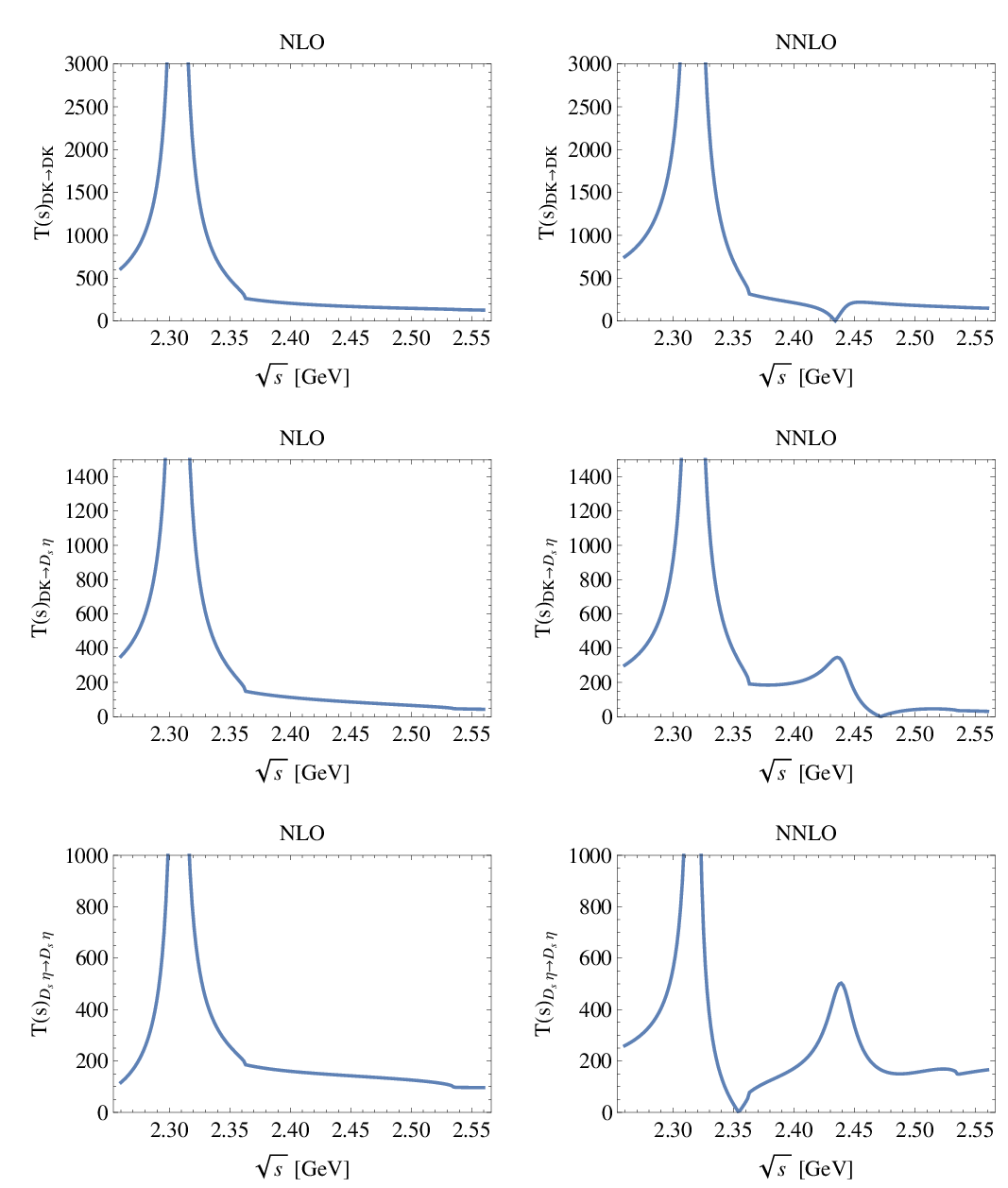
For the coupled-channel system, in addition to the pole at GeV on the physical sheet, which corresponds to and was used as a condition to constrain the parameters, using the central values of the parameters we also found a pair of poles with a small but nonvanishing imaginary part on the second Riemann sheet, GeV. The only work which reported an analogous pole is Ref. [33], where a virtual state at GeV below threshold on the second Riemann sheet was reported in an NLO calculation including and channels. We check whether such a pole exists using the parameters from the NLO fits in Ref. [25], and found that only part of the allowed parameter space allows for the pole on the unphysical Riemann sheet. Moreover, the effect of this virtual state pole located at GeV on the physical amplitude is negligible in the NLO calculation, as can be seen from the left column of Fig. 4. However, the pole on the second Riemann sheet in the NNLO calculation can have a non-negligible effect on specific physical amplitudes, as shown in the right column of Fig. 4. These different behaviors are mainly due to different locations of the poles. Nevertheless, we see that the lattice data on the scattering lengths are insufficient to constrain the parameters, and as a result, calculations at different orders may even have a sizeable discrepancy in amplitudes not far from thresholds. More lattice data on scattering observables are needed to better pin down the LECs.
In addition, we also found a pair of poles GeV on the second Riemann sheet which are not included in Table 4. They have a negligible effect on physical amplitudes and would disappear if the - and -channels are turned off. Likewise, we do not include the following poles in Table 4 since they are located far from the physical region and have little effect: poles at GeV and GeV on the third Riemann sheet for and , respectively; poles at GeV on the second Riemann sheet in the channel.
It is well-known that the unitarization approach, relying on right-hand unitarity and the on-shell approximation, has the problem of violation of unitarity when the left-hand cut occurs in the on-shell potential. For instance, the left-hand cut in the amplitude leads a violation of unitarity for the scattering in the – coupled-channel system [59, 60]. 77 7 As pointed out by Refs [61, 59], the unitarity violation is numerically small in the – case, hence no serious problem was caused there. The same unitarity violation happens to the scattering with , which has three coupled channels: , and . One of the left-hand cuts from the inelastic channel amplitude, from ( GeV)2 to ( GeV)2, overlaps with the right-hand cut starting from the threshold, which can be verified by the discontinuity across the real axis below the threshold. Although this left-hand cut is not numerically important, its presence together with other left-hand cuts and right-hand cuts make the whole real axis nonanalytic. Since Eq. (23) was derived using the method neglecting the left-hand cuts, its continuation to the complex plane near the left-hand cut is untrustworthy. As a result, the coupled-channel amplitudes obtained from Eq. (23) do not have the correct analytic properties even in the relevant energy region. Consequently, a pair of pole at are found on the first Riemann sheet for the coupled-channel amplitude. As we know, poles on the first Riemann sheet can only be located on the real axis below the lowest threshold, which are associated with bound states. A pole on the first sheet with a nonvanishing imaginary part or above the lowest threshold is inconsistent with causality. The appearance of the pole on the first sheet in the coupled-channel is due to the existence of the coupled-channel cut. The left-hand cuts stem from the one-loop potentials, and are absent in the NLO cases.
If we consider only the single-channel for , there is no such a problem as it comes from the left-hand cut of the inelastic channels. We searched for poles in the single-channel amplitude, and found a pair of poles in the second Riemann sheet given in Table 5,88 8 Notice that the poles found in both the single-channel and coupled-channel unitarized NLO amplitudes are similar to each other in Ref. [13]. corresponding to the lower pole at GeV of the two-pole structure of advocated in Ref. [34].
In addition, we also investigated the pole movements with varying pion masses. The pion mass dependence trajectories of the poles can provide us with useful information about the properties of the different states, as discussed, e.g., in Ref. [62]. The trajectory for the pole corresponding to is plotted in Fig. 5. The pole positions on the first Riemann sheet, which are identified as the pole mass, are shown as the solid line. The dotted line stands for the trajectory of the threshold. From Fig. 5, one can see that the always stays below the corresponding threshold as a bound state for a wide range of . The trajectory of is quite similar to the NLO fit result, as shown in Ref. [33].


On the contrary, the pion mass dependence trajectory of the pole around on the second Riemann sheet for the single-channel in Table 5 is quite complicated, as shown in Fig. 6. As the value of increases from , both the real and imaginary parts of the pole tend to decrease on the second Riemann sheet. At some point around , the real part of the pole becomes lower than the corresponding threshold. When increases to around , the pair of poles hits the real axis below the threshold and these become two virtual states on the second Riemann sheet. If we further increase the pion mass, one of the virtual poles would move along the real axis away from the threshold, while the other one moves towards the threshold and becomes a bound state of the first Riemann sheet at . If we keep increasing , both the virtual state and bound state move away from the threshold along the real axis. The behavior of the pole is similar to the corresponding ones in Refs. [13, 33] as well as the pion mass dependence of the in Ref. [63]. It is general for -wave states.
IV Summary and conclusions
We have calculated the potential for the scattering of Goldstone bosons off charmed mesons, including the charmed vector mesons as explicit degrees of freedom, up to the NNLO in a framework of covariant ChPT. We explicitly show that the UV divergences and the so-called power counting breaking terms from the one-loop potentials can be absorbed by a redefinition of the LECs. In the EOMS scheme, we obtained the scattering potentials possessing the good properties, i.e., they are free of UV divergences and power counting violating terms. In order to describe the -wave scattering lengths at high pion masses and to study the possible dynamically generated resonances that are absent in the Lagrangian, e.g. the , at relatively high energies, which is the nonperturbative effect, a unitarization procedure is employed.
In order to determine the LECs, we performed fits to scattering lengths in a few channels computed in lattice QCD at various unphysical pion masses. Since the lattice simulations are performed with fixed charm and strange quark masses with varying up and down quark masses, we derived the corresponding pion mass dependence of the scattering lengths by extrapolation of the involved masses and the pion decay constant. For an easy comparison to the previous case without including explicitly, we used a similar fit procedure as in Ref. [32]. It turns out that, for UChPT-6(b), the current fit result is quite close to the previous one which was done without explicit vector charmed mesons. It is thus a firm conclusion that the contribution to the -wave scattering in the threshold region is negligible.
Based on the small contribution of the to the scattering potentials, we investigated possible dynamically generated resonances using the unitarized scattering amplitudes without explicit by analytic continuation. It is worth noticing that a pair of poles with nonvanishing imaginary parts are found on the physical Riemann sheet in the coupled-channel amplitude, which are at odds with causality. The issue is caused by the coupled-channel left-hand cut, which is not taken into account in the unitarization procedure we used. It may be avoided by using a single-channel potential if we only focus on the region near the threshold. In the end, we studied the trajectories of the poles corresponding to the and a resonance in channel with varying the pion mass. They exhibit similar behaviors as in the NLO case given by Ref. [33]. To summarize, the LECs are badly determined due to the scarcity of available data. Thus to come to firmer conclusions, more lattice data are required, as also concluded from investigations based on the resonance-exchange model and -matrix properties in Ref. [64].
Acknowledgements
We would like to thank Jiunn-Wei Chen, Jambul Gegelia and Zhi-Hui Guo for helpful discussions. MLD acknowledges the warm hospitality of the ITP of CAS where part of this work was done. This work is supported in part by DFG and NSFC through funds provided to the Sino-German CRC 110 “Symmetries and the Emergence of Structure in QCD” (NSFC Grant No. 11621131001, DFG Grant No. TRR110), by NSFC (Grant No. 11647601), by the Thousand Talents Plan for Young Professionals, by the CAS Key Research Program of Frontier Sciences (Grant No. QYZDB-SSW-SYS013), and by the CAS President’s International Fellowship Initiative (PIFI) (Grant No. 2017VMA0025).
Appendix A Renormalization of the LECs within EOMS scheme
In this appendix, we use the following notations for the chiral limit masses of and : and . Following Ref. [65], the -point one-loop integrals are defined by
The one-, two- and three-point one-loop scalar integrals are denoted by , and as follows:
| (63) |
A.1 -functions
The -functions in Eq. (19) read
| (64) |
A.2 Coefficients of finite shifts
In this appendix, we express the EOMS subtractions in terms of the standard loop function. The explicit coefficients of the finite shifts in Eq. (20) are
| (65) | |||||
| (66) | |||||
| (67) | |||||
| (68) | |||||
| (69) | |||||
| (70) | |||||
| (71) | |||||
Here the involved scalar one-loop integrals stand for their finite parts only, which are obtained from the original ones, defined in Eq. (A), by performing the subtraction.
References
- [1] A. J. Bevan et al. [BaBar and Belle Collaborations], Eur. Phys. J. C 74, 3026 (2014) [arXiv:1406.6311 [hep-ex]].
- [2] B. Aubert et al. [BaBar Collaboration], Phys. Rev. Lett. 90, 242001 (2003) [hep-ex/0304021].
- [3] P. Krokovny et al. [Belle Collaboration], Phys. Rev. Lett. 91, 262002 (2003) [hep-ex/0308019].
- [4] D. Besson et al. [CLEO Collaboration], Phys. Rev. D 68, 032002 (2003) Erratum: [Phys. Rev. D 75, 119908 (2007)] [hep-ex/0305100].
- [5] R. Aaij et al. [LHCb Collaboration], Phys. Rev. D 91, no. 9, 092002 (2015) Erratum: [Phys. Rev. D 93, no. 11, 119901 (2016)] [arXiv:1503.02995 [hep-ex]].
- [6] H. X. Chen, W. Chen, X. Liu, Y. R. Liu and S. L. Zhu, doi:10.1088/1361-6633/aa6420 [arXiv:1609.08928 [hep-ph]].
- [7] T. Barnes, F. E. Close and H. J. Lipkin, Phys. Rev. D 68, 054006 (2003) [hep-ph/0305025].
- [8] E. E. Kolomeitsev and M. F. M. Lutz, Phys. Lett. B 582, 39 (2004) [hep-ph/0307133].
- [9] F.-K. Guo, P. N. Shen, H. C. Chiang, R. G. Ping and B. S. Zou, Phys. Lett. B 641, 278 (2006) [hep-ph/0603072].
- [10] D. Gamermann, E. Oset, D. Strottman and M. J. Vicente Vacas, Phys. Rev. D 76, 074016 (2007) [hep-ph/0612179].
- [11] J. Hofmann and M. F. M. Lutz, Nucl. Phys. A 733, 142 (2004) [hep-ph/0308263].
- [12] F.-K. Guo, C. Hanhart, S. Krewald and U.-G. Meißner, Phys. Lett. B 666, 251 (2008) [arXiv:0806.3374 [hep-ph]].
- [13] F.-K. Guo, C. Hanhart and U.-G. Meißner, Eur. Phys. J. A 40, 171 (2009) [arXiv:0901.1597 [hep-ph]].
- [14] M. Cleven, F.-K. Guo, C. Hanhart and U.-G. Meißner, Eur. Phys. J. A 47, 19 (2011) [arXiv:1009.3804 [hep-ph]].
- [15] M. Cleven, H. W. Grießhammer, F.-K. Guo, C. Hanhart and U.-G. Meißner, Eur. Phys. J. A 50, 149 (2014) [arXiv:1405.2242 [hep-ph]].
- [16] G. Burdman and J. F. Donoghue, Phys. Lett. B 280, 287 (1992).
- [17] M. B. Wise, Phys. Rev. D 45, no. 7, R2188 (1992).
- [18] T. M. Yan, H. Y. Cheng, C. Y. Cheung, G. L. Lin, Y. C. Lin and H. L. Yu, Phys. Rev. D 46, 1148 (1992) Erratum: [Phys. Rev. D 55, 5851 (1997)].
- [19] J. A. Oller and U.-G. Meißner, Phys. Lett. B 500, 263 (2001) [hep-ph/0011146].
- [20] G. Moir, M. Peardon, S. M. Ryan, C. E. Thomas and L. Liu, JHEP 1305, 021 (2013) [arXiv:1301.7670 [hep-ph]].
- [21] K. Cichy, M. Kalinowski and M. Wagner, PoS LATTICE 2015, 093 (2015) [arXiv:1510.07862 [hep-lat]].
- [22] C. Liu, X. Feng and S. He, Int. J. Mod. Phys. A 21, 847 (2006) [hep-lat/0508022].
- [23] M. Lage, U.-G. Meißner and A. Rusetsky, Phys. Lett. B 681, 439 (2009) [arXiv:0905.0069 [hep-lat]].
- [24] L. Liu, H. W. Lin and K. Orginos, PoS LATTICE 2008, 112 (2008) [arXiv:0810.5412 [hep-lat]].
- [25] L. Liu, K. Orginos, F.-K. Guo, C. Hanhart and U.-G. Meißner, Phys. Rev. D 87, no. 1, 014508 (2013) [arXiv:1208.4535 [hep-lat]].
- [26] D. Mohler, S. Prelovsek and R. M. Woloshyn, Phys. Rev. D 87, no. 3, 034501 (2013) [arXiv:1208.4059 [hep-lat]].
- [27] D. Mohler, C. B. Lang, L. Leskovec, S. Prelovsek and R. M. Woloshyn, Phys. Rev. Lett. 111, no. 22, 222001 (2013) [arXiv:1308.3175 [hep-lat]].
- [28] C. B. Lang, L. Leskovec, D. Mohler, S. Prelovsek and R. M. Woloshyn, Phys. Rev. D 90, no. 3, 034510 (2014) [arXiv:1403.8103 [hep-lat]].
- [29] G. Moir, M. Peardon, S. M. Ryan, C. E. Thomas and D. J. Wilson, JHEP 1610, 011 (2016) [arXiv:1607.07093 [hep-lat]].
- [30] P. Wang and X. G. Wang, Phys. Rev. D 86, 014030 (2012) [arXiv:1204.5553 [hep-ph]].
- [31] M. Altenbuchinger, L.-S. Geng and W. Weise, Phys. Rev. D 89, no. 1, 014026 (2014) [arXiv:1309.4743 [hep-ph]].
- [32] D.-L. Yao, M.-L. Du, F.-K. Guo and U.-G. Meißner, JHEP 1511, 058 (2015) [arXiv:1502.05981 [hep-ph]].
- [33] Z. H. Guo, U.-G. Meißner and D.-L. Yao, Phys. Rev. D 92, no. 9, 094008 (2015) [arXiv:1507.03123 [hep-ph]].
- [34] M. Albaladejo, P. Fernandez-Soler, F.-K. Guo and J. Nieves, Phys. Lett. B 767, 465 (2017) [arXiv:1610.06727 [hep-ph]].
- [35] C. Patrignani et al. [Particle Data Group], Chin. Phys. C 40, no. 10, 100001 (2016).
- [36] J. Gasser, M. E. Sainio and A. Svarc, Nucl. Phys. B 307, 779 (1988).
- [37] E. E. Jenkins and A. V. Manohar, Phys. Lett. B 255, 558 (1991).
- [38] V. Bernard, N. Kaiser, J. Kambor and U.-G. Meißner, Nucl. Phys. B 388, 315 (1992).
- [39] T. Becher and H. Leutwyler, Eur. Phys. J. C 9, 643 (1999) [hep-ph/9901384].
- [40] T. Fuchs, J. Gegelia, G. Japaridze and S. Scherer, Phys. Rev. D 68, 056005 (2003) [hep-ph/0302117].
- [41] J. M. Alarcon, J. Martin Camalich and J. A. Oller, Annals Phys. 336, 413 (2013) [arXiv:1210.4450 [hep-ph]].
- [42] Y. H. Chen, D.-L. Yao and H. Q. Zheng, Phys. Rev. D 87, 054019 (2013) [arXiv:1212.1893 [hep-ph]].
- [43] D.-L. Yao, D. Siemens, V. Bernard, E. Epelbaum, A. M. Gasparyan, J. Gegelia, H. Krebs and U.-G. Meißner, JHEP 1605, 038 (2016) [arXiv:1603.03638 [hep-ph]].
- [44] Y. R. Liu, X. Liu and S. L. Zhu, Phys. Rev. D 79, 094026 (2009) [arXiv:0904.1770 [hep-ph]].
- [45] L. S. Geng, N. Kaiser, J. Martin-Camalich and W. Weise, Phys. Rev. D 82, 054022 (2010) [arXiv:1008.0383 [hep-ph]].
- [46] V. Bernard, N. Kaiser, U.-G. Meißner and A. Schmidt, Z. Phys. A 348, 317 (1994) [hep-ph/9311354].
- [47] M.-L. Du, F.-K. Guo and U.-G. Meißner, J. Phys. G 44, 014001 (2017) [arXiv:1607.00822 [hep-ph]].
- [48] M.-L. Du, F.-K. Guo and U.-G. Meißner, JHEP 1610, 122 (2016) [arXiv:1609.06134 [hep-ph]].
- [49] Z. H. Guo and J. A. Oller, Phys. Rev. D 84, 034005 (2011) [arXiv:1104.2849 [hep-ph]].
- [50] J. Gasser and H. Leutwyler, Nucl. Phys. B 250, 465 (1985).
- [51] H. Krebs, E. Epelbaum and U.-G. Meißner, Phys. Lett. B 683, 222 (2010) [arXiv:0905.2744 [hep-th]].
- [52] J. R. Peláez, Phys. Rept. 658, 1 (2016) [arXiv:1510.00653 [hep-ph]].
- [53] J. A. Oller and E. Oset, Nucl. Phys. A 620, 438 (1997) Erratum: [Nucl. Phys. A 652, 407 (1999)] [hep-ph/9702314].
- [54] J. A. Oller, E. Oset and J. R. Peláez, Phys. Rev. D 59, 074001 (1999) Erratum: [Phys. Rev. D 60, 099906 (1999)] Erratum: [Phys. Rev. D 75, 099903 (2007)] [hep-ph/9804209].
- [55] D. R. Entem and J. A. Oller, arXiv:1610.01040 [nucl-th].
- [56] J. A. Oller and E. Oset, Phys. Rev. D 60, 074023 (1999) [hep-ph/9809337].
- [57] P. C. Bruns and U.-G. Meißner, Eur. Phys. J. C 40, 97 (2005) [hep-ph/0411223].
- [58] A. Walker-Loud et al., Phys. Rev. D 79, 054502 (2009) [arXiv:0806.4549 [hep-lat]].
- [59] A. Gomez Nicola and J. R. Peláez, Phys. Rev. D 65, 054009 (2002) [hep-ph/0109056].
- [60] L. Y. Dai, X. G. Wang and H. Q. Zheng, Commun. Theor. Phys. 57, 841 (2012) [arXiv:1108.1451 [hep-ph]].
- [61] F. Guerrero and J. A. Oller, Nucl. Phys. B 537, 459 (1999) Erratum: [Nucl. Phys. B 602, 641 (2001)] [hep-ph/9805334].
- [62] C. Hanhart, J. R. Peláez and G. Rios, Phys. Lett. B 739, 375 (2014) [arXiv:1407.7452 [hep-ph]].
- [63] C. Hanhart, J. R. Peláez and G. Ríos, Phys. Rev. Lett. 100, 152001 (2008) [arXiv:0801.2871 [hep-ph]].
- [64] M.-L. Du, F.-K. Guo, U.-G. Meißner and D.-L. Yao, Phys. Rev. D 94, no. 9, 094037 (2016) [arXiv:1610.02963 [hep-ph]].
- [65] A. Denner, Fortsch. Phys. 41, 307 (1993) [arXiv:0709.1075 [hep-ph]].