Modeling, Analysis, and Optimization of Coded Caching in Small-Cell NetworksThanks: This work has been accepted in part by IEEE ICC 2017 [1].Thanks: The authors are with the Department of Electronic Engineering, Shanghai Jiao Tong University, Shanghai, China. Emails: {manchester_red, mxtao}@sjtu.edu.cn.
Abstract
Coded caching is able to exploit accumulated cache size and hence superior to uncoded caching by distributing different fractions of a file in different nodes. This work investigates coded caching in a large-scale small-cell network (SCN) where the locations of small base stations (SBSs) are modeled by stochastic geometry. We first propose a content delivery framework, where multiple SBSs that cache different coded packets of a desired file transmit concurrently upon a user request and the user decodes the signals using successive interference cancellation (SIC). We characterize the performance of coded caching by two performance metrics, average fractional offloaded traffic (AFOT) and average ergodic rate (AER), for which a closed-form expression and a tractable expression are derived, respectively, in the high signal-to-noise ratio region. We then formulate the coded cache placement problem for AFOT maximization as a multiple-choice knapsack problem (MCKP). By utilizing the analytical properties of AFOT, a greedy but optimal algorithm is proposed. We also consider the coded cache placement problem for AER maximization. By converting this problem into a standard MCKP, a heuristic algorithm is proposed. Analytical and numerical results reveal several design and performance insights of coded caching in conjunction with SIC receiver in interference-limited SCNs.
Index Terms:
Coded caching, successive interference cancellation, stochastic geometry, small-cell networks, knapsack problem.I Introduction
I-A Motivation and Related Works
The global mobile data traffic has undergone a fundamental shift from voices and messages to rich content distributions, such as video streaming and application downloads. By prefetching popular contents during off-peak times at the edge of wireless networks, such as small base stations (SBSs), helper nodes, and user devices, wireless caching can alleviate peak-hour network congestion, provide traffic offloading, and improve users’ quality of experience [2, 3, 4]. It thus has attracted great attention recently.
Cache-enabled wireless networks operate in two phases in general, i.e., cache placement and content delivery [5]. Cache placement is to place or update contents in each cache-enabled node subject to the storage size. Content delivery is to deliver contents upon user requests conditioned on cache state as well as network channel condition. While the design of the content delivery phase can be decoupled from the cache placement phase once the cache placement strategy is given, e.g., [6, 7, 8], the design of the cache placement phase is tightly coupled with the content delivery phase in wireless networks, e.g. [9, 10, 11, 12, 13, 14, 15]. In this work, we are interested in the cache-enabled small-cell networks (SCNs), where each SBS is equipped with a local cache and can serve user requests based on its cached contents. In a deterministic SCN with fixed connection topology, the cache placement problem is NP-hard [16]. Alternatively, the authors in [17, 18, 11, 12, 13, 14] apply tools from stochastic geometry to study the cache placement problem by assuming that the locations of SBSs follow a homogeneous Poisson point process (HPPP) in a large-scale SCN. In particular, the authors in [17] analyze the outage probability and the average content delivery rate when each SBS stores the most popular contents and each user is only associated with the nearest SBS. The authors in [18] analyze the average ergodic rate and the outage probability with the most popular contents caching in a three-tier heterogeneous network. The works [11, 12, 13, 14] show that caching the contents randomly with the optimized probabilities has performance improvement, e.g., the cache hit probability, the successful offloading probability, and the average success probability of content delivery, over caching the most popular contents since each user can be covered by multiple SBSs.
Recently, it is shown in [15, 16, 19, 20, 21, 22, 23] that partitioning each file into multiple segments and caching different segments of a file in different SBSs can further enhance cache efficiency. This is known as coded caching in [16]. When a user submits a file request, the file shall be delivered to the user from multiple nearby SBSs that have cached the different segments of the file, thereby exploiting the accumulated cache size. The work [15] proposes a combined coded/uncoded caching strategy in disjoint cluster-centric SCN and analyzes the successful content delivery probability for a user located at the cluster center. In the combined caching strategy, part of the cache space in each SBS is reserved for the most popular contents and the remaining is to cache different partitions of the less popular contents. This strategy is, however, a heuristic one and cannot fully exploit the accumulated cache size. In [16, 19, 20], the maximum distance separable (MDS)-coded caching schemes are considered. With an MDS code, each file is split into fragments and then encoded into coded packets. Any set of coded packets is sufficient to recover the file. The works [16] and [19] formulate the optimal MDS-coded cache placement problems to minimize the average file download time and the average backhaul rate, respectively. Compared with [19], the work [20] considers a more practical scenario with heterogeneous file and cache sizes. In [21, 22, 23], random linear network coding (RLNC) is applied to generate and store coded packets in SBSs. Similar to MDS codes, when a file is split into fragments and the coding coefficients in RLNC are randomly selected from a large field, the file can be recovered from any coded packets with high probability. All these works on MDS- or RLNC-coded caching in SCNs however assume an ideal error-free transmission with fixed connection topology in the content delivery phase. Coded caching strategy in a realistic SCN with channel fading and inter-cell interferences remains uninvestigated.
I-B Contributions
In this work, we apply stochastic geometry to model, analyze, and optimize coded caching in a cache-enabled SCN. The locations of SBSs are assumed to follow an HPPP on a plane. Each file is first partitioned into fragments and then encoded using either MDS codes or RLNC into an arbitrarily large number of coded packets, such that any set of coded packets is enough to recover the original file. Each SBS stores a certain number of different coded packets for each file subject to a finite cache size. When a user requests a file, the user will be associated with a sufficient number of SBSs that have cached the coded packets of the desired file for file downloading. The main contributions of this work are summarized as follows.
- •
A content delivery framework with SIC receiver: We propose a new content delivery framework for coded caching, where multiple SBSs that cache the different coded packets of a desired file transmit concurrently upon a user request and the user decodes the signals successively using a successive interference cancellation (SIC)-based receiver. The number of concurrently transmitting SBSs, or equivalently, the number of SIC decoding layers, depends on the number of coded packets of the desired file cached in each SBS. We also obtain a closed-form expression to tightly approximate the success probability of each SIC decoding layer for a typical user in the high signal-to-noise ratio (SNR) region.
- •
New performance metrics and analysis: We introduce and analyze two performance metrics for coded caching in SCNs. One is the average fractional offloaded traffic (AFOT). It measures the average fraction of each file that can be successfully delivered by the cache-enabled SBSs and hence offloaded from the core network at a given target SIC decoding threshold. Based on the success probability of each SIC decoding layer, we obtain a closed-form expression of AFOT. We show that the fractional offloaded traffic (FOT) for a given file is an increasing, concave, and piece-wise arithmetic sequence as the number of its coded packets cached in each SBS increases. The other is the average ergodic rate (AER), which characterizes the average ergodic data rate of a typical user achievable over the cache-enabled SBSs. We then obtain a tractable expression for AER.
- •
Optimization of coded cache placement: We formulate two coded cache placement problems for AFOT maximization and AER maximization, respectively. The AFOT maximization problem is a multiple-choice knapsack problem (MCKP). Utilizing the analytical properties of AFOT, we propose a greedy-based algorithm that finds the global optimal solution efficiently. In the limiting case where each file can be split into infinite number of fragments, we also reformulate the discrete problem for AFOT maximization into a continuous one, which is shown to be convex. The optimal solution of the continuous problem provides a performance upper bound for the discrete problem. It also prompts us to propose a low-complexity algorithm with high performance for the discrete problem. To solve the coded cache placement problem for AER maximization, we transform it into a standard MCKP, for which a heuristic algorithm is proposed.
- •
Performance and design insights via numerical simulations: Extensive numerical results demonstrate that it is good enough to split each file into not-so-large, e.g., , fragments for coded caching to approach the performance upper bound of AFOT. Results also show that coded caching can well exploit the accumulated cache size among neighboring SBSs and hence significantly offload more traffic than uncoded caching when the decoding threshold for each SIC decoding layer is low. On the other hand, the gain of coded caching vanishes in terms of the AER performance unless the file popularity distribution is close to uniform.
I-C Paper Organization
This paper is organized as follows. We present the network model, coded caching with SIC receiver, and the performance metrics, namely, AFOT and AER in Section II. We analyze the proposed performance metrics in Section III and formulate the coded cache problems into MCKP to optimize the caching vector in Section IV. Numerical results are presented in Section V and Section VI concludes the paper.
II System Model
II-A Network Model
We consider a cache-enabled SCN where the SBSs and users are spatially distributed on a plane according to two independent HPPPs with densities and , respectively. Each SBS is equipped with a local cache and serves mobile users with its cached contents. All SBSs and users are equipped with single antenna. Without loss of generality, we focus on the analysis at a typical user . We define as the -th nearest SBS to with distance denoted by . The network is assumed to be fully loaded so that each SBS transmits signals all the time, which is the worst-case scenario for performance analysis. There is also a tier of macro base stations (MBSs) in the network, which are connected to the core network via backhaul links and communicate with users only when the user demands cannot be satisfied by SBSs. We assume that the MBSs and SBSs operate over non-overlapping frequency bands to avoid the inter-tier interference.
In the downlink channel, we consider both large-scale fading and small-scale fading. The large-scale fading is modeled by a standard distance-dependent power law pathloss attenuation. For small-scale fading, Rayleigh fading is considered. The transmission power of each SBS is . Hence, the received signal power at from can be written as , where is the complex-valued channel coefficient from to and is the pathloss exponent.
II-B Coded Caching Model
Consider a content library consisting of files, denoted by . Each file has the same size of bits. The popularity of is denoted as , for , satisfying and . Without loss of generality, we assume .
A coded caching scheme similar to [19] is adopted in this work. Each file in the content library is split into equal-sized fragments, for being any positive integer. The fragments of each file are then encoded into an arbitrarily large number of packets. Here, we mention fragment as the original part of a file and packet as the coded part of a file. We do not restrict to any specific coding scheme and only require that the file can be decoded successfully from any coded packets. In practice, this requirement can be satisfied by using MDS codes or satisfied with high probability by using RLNC.
Each SBS has a local cache and can store up to bits . In the cache placement phase, each SBS stores different coded packets of , for each . We refer to as the caching vector, which shall be optimized subject to the following cache size constraint:
| (1) |
The specific packet storing approach depends on the coding scheme in the cache placement phase. For example, if an MDS code with rate is used, where is the number of the fragments that each file is partitioned into and is the number of the coded packets based on the fragments, we can use graph coloring to store the coded packets in each SBS. In specific, we first tessellate the considered network area into -th order Voronoi regions, each of which is associated with SBSs so that any point in this region is closer to these SBSs than any other SBS in the network area. Then, we construct a graph, where each SBS is represented by a vertex and every pair of SBSs that belong to the same -th order Voronoi region are connected with an edge. Let every distinct set of coded packets be represented by a color. The maximum number of colors is . We then color the vertices of the graph so that no adjacent vertices share the same color, which is clearly feasible when is sufficiently large. By this coloring-based packet storing approach, the SBSs in each Voronoi region are guaranteed to have different coded packets. On the other hand, if RLNC is used by each SBS to encode the fragments with the coding coefficients independently and uniformly selected from a large field, the coded packets generated and stored in each SBS are ensured to be linearly independent with high probability. In specific, let denote the finite field where the random coding coefficients are chosen from and let denote the event that any coded packets collected from any SBSs in the network can recover the uncoded fragments and hence the complete file. According to [21], we have that . It is seen that when is large enough, is very large.
II-C Content Request and Delivery Model
Each user requests for one file independently with probability according to the file popularity distribution. Consider that the typical user sends a request for , . If , i.e., no SBS has stored any part of , will be served by an MBS, which is assumed to have access to all files through backhaul link. If , will be associated with the set of nearest SBSs, denoted as , to retrieve enough number of coded packets for the file decoding11 1 The work can be extended to other user association strategies by considering different practical constraints. For instance, due to the limited SIC decoding capability, a user may only be associated with a maximum of nearest SBSs. Likewise, due the the large signal attenuation, a user may only be associated with the SBSs that are within a given distance.. The SBSs transmit their own cached packets concurrently over the same resource block. Users adopt SIC-based receiver to decode the signals from multiple SBSs successively in the descending order of the average received signal strength as in [15]. More specifically, the signal from the nearest SBS is decoded first and, if successful, subtracted from the received signal, then the signal from the second nearest SBS is decoded based on the residue received signal. The procedure repeats till the signals from all the SBSs in are decoded. The total number of decoding layers in the SIC-based receiver (equivalent to the total number of SBSs that transmit concurrently to ) is . This number varies between and , depending on the different choices of for . Thus, the coding parameter for content caching sets the highest possible SIC receiver complexity.
Note that to decode the signal from , the signals from must be decoded and subtracted first from the received signal, and then only the signals from and beyond are seen as interferences. Define as the set of SBSs whose distances to are larger than or equal to , for . Then, the residue received signal for decoding the signal from is given by
| (2) |
where denotes the transmitted symbol from and is assumed independent for different ’s, and is the complex additive white Gaussian noise of power .
We focus on the interference-limited network where the noise can be neglected. The signal-to-interference ratio (SIR) for decoding is given by
| (3) |
II-D Performance Metrics
In our work, we shall measure the performance of coded caching using two metrics, namely, the average fractional offloaded traffic (AFOT) and the average ergodic rate (AER). The former characterizes the average fraction of each file that can be successfully delivered by the cache-enabled SBSs and hence offloaded from the core network at a given target SIC decoding threshold. The latter characterizes the average ergodic data rate of the typical user achievable over the cache-enabled SBSs.
II-D1 Average Fractional Offloaded Traffic (AFOT)
We first define the successful transmission probability of each decoding layer at a common SIR threshold . The signal from can only be decoded successfully if after the signals from are all decoded and subtracted successfully. The probability of this event is referred to as the success probability of the -th decoding layer, denoted by
| (4) |
Otherwise, if , the decoding of fails and the SIC process terminates. The remaining coded packets will be acquired from an MBS for to recover the complete requested file.
Consider that sends a request for and coded packets of the file are stored in each SBS. As mentioned above, the user can only decode the packets from after all the transmissions from the first nearest SBSs are successful. Once the decoding of the -th layer fails, the SIC-based decoding process terminates. Then, only coded packets of can be offloaded by the SBSs. If all the decoding layers are successful, the entire file can be offloaded. Therefore, the fractional offloaded traffic (FOT) for , denoted as , is given by
| (5) |
By averaging over all files in , the AFOT, denoted as , is given by
| (6) |
Remark 1.
We would like to highlight that the decoding threshold in (4) is set as a constant, independent of the decoding layers in the SIC receiver. At first glance, this means that it only takes seconds to deliver the requested file (no matter it succeeds or not) since each SBS only transmits bits, where is the target delivery time of a file of bits in the traditional uncoded caching scheme with channel bandwidth of Hz. However, SBSs are involved in delivering . The accumulated time resource consumed by delivering thus becomes , which is equal to or slightly larger than . Thus, having a constant in (4) ensures a fair comparison between coded and uncoded caching in terms of the total network resource consumption.
II-D2 Average Ergodic Rate (AER)
Again, consider that sends a request for and coded packets of the file are stored in each SBS. Here, we assume that each SBS adopts a rate-adaptive transmission strategy so that the signals transmitted from all the SBSs in are always decodable using the SIC receiver when . Since each SBS in needs to transmit the same amount of information bits to , the actual transmission rate of each SBS is chosen according to the worst SIR among all decoding layers in (3). Thus, the ergodic rate achievable by when requesting , denoted as bits/s/Hz, is given by
| (7) |
By averaging over all files in , the AER of the typical user achievable over the cache-enabled SBSs, denoted as bits/s/Hz, is given by
| (8) |
III Performance Analysis
In this section, we shall analyze the performance of coded caching using the AFOT and AER defined in the previous section. Especially, exploring the structural properties of FOT will benefit the coded caching optimization problem for AFOT maximization in Section IV.
III-A Analysis of Fractional Offloaded Traffic
We first obtain a closed-form expression for the success probability of the -th decoding layer , defined in (4), then apply it to obtain a closed-form expression for defined in (5).
Lemma 1.
The success probability of the -th decoding layer with SIC receiver can be approximated as
| (9) |
where is the complementary incomplete Beta function.
Proof.
Please see Appendix A. ∎
We shall demonstrate via simulation in Section V-A that the closed-form expression in Lemma 1 is a tight approximation of the true successful transmission probability of SBS after the signals from are all successfully decoded and subtracted.
Lemma 2.
The fractional offloaded traffic of with caching parameter is given by
| (10) |
where
| (11) |
Proof.
Please see Appendix B. ∎
By substituting (10) into (6), a closed-form expression of AFOT for any given caching vector is readily obtained.
Now we analyze the properties of , which will be essential for cache placement optimization in the next section.
Lemma 3.
is a piece-wise arithmetic sequence, for .
Proof.
Define an integer set and . For example, and when . Then, we have , . Thus, for all ’s such that , the first difference of is given by
| (12) |
Equation (12) indicates that when multiple ’s all belong to , the difference of , i.e., , is same and thus is an arithmetic sequence. If but , for , then we denote the first difference as . Thus, is a piece-wise arithmetic sequence with first difference given by when or when and . The Lemma is thus proven. ∎
| 0 | 1 | 2 | 3 | 4 | 5 | 6 | 7 | 8 | |
| 8 | 4 | 3 | 2 | 1 | |||||
By Lemma 3 and its proof, we can construct a difference table of , for , termed as the offloaded traffic difference table. An example with is shown in TABLE I. Here, . For any given , an offloaded traffic difference table can be constructed. We shall use this table to design a greedy-based optimal algorithm and a low-complexity algorithm with high performance for the cache placement problem for AFOT maximization in the next section. The total number of distinct ’s for general , denoted as , depends on the size of set , i.e., the number of piece-wise regions for , which is usually much smaller than . For example, , and . When , . The proof is skipped due to the page limit.
Now, we consider the limiting case where . That means the file size is very large so that each file can be split into infinite number of fragments. Define a new variable . When , can be relaxed as a continuous variable within . Then, the discrete function in (10) can be relaxed as a continuous function :
| (13) |
The properties of are summarized in the following lemma.
Lemma 4.
is an increasing, concave and piece-wise linear function of , for .
Proof.
Please see Appendix C. ∎
For any given , can be viewed as the sampled function of at sampling instance . Since is increasing and concave by Lemma 4, is also increasing and concave. We thus have the following corollary.
Corollary 1.
is an increasing and concave sequence, i.e., , for .

III-B Analysis of Ergodic Rate
By using the definition in (7), the ergodic rate of when requesting can be expressed in a tractable form below.
Lemma 5.
The ergodic rate for with caching parameter is given by
| (14) |
where is given in (11) by letting and .
Proof.
Please see Appendix D. ∎
IV Optimization of Coded Caching
In this section, we would like to maximize the AFOT and AER, respectively, by optimizing the caching vector . In the AFOT optimization, we first study the discrete optimization problem when the coding parameter is finite, and then study the continuous optimization problem when . In the AER optimization, we only consider the discrete case when is finite.
IV-A Discrete Problem for AFOT Optimization
The objective is to maximize the AFOT in (6) by optimizing the caching vector subject to the cache size constraint (1) at a given finite . This is formulated as follows.
Problem 1 (Discrete Coded Cache Problem for AFOT Maximization).
| (15) |
Before solving Problem 1, we shall present a property of the optimal caching vector .
Theorem 1.
The optimal caching vector of Problem 1 satisfies that , for any given file popularities .
Proof.
Please see Appendix E. ∎
Theorem 1 matches the common intuition that more cache size should be allocated to more popular contents when the total cache size is limited.
Note that Problem 1 is a multiple-choice knapsack problem (MCKP) [24, Chapter 11], which is known to be NP-hard. The problem can be interpreted as follows. Consider a knapsack with capacity of packets and a set of files each containing packets. The size of each file packet is the same but the profit of each file packet varies according to the number of packets as well as the index of file. Based on the properties of analyzed in Section III-A and the property of in Theorem 1, we design a greedy but optimal algorithm as outlined in Algorithm 1 to solve Problem 1.
- •
Store packets for each of the most popular files in each SBS, i.e., ;
- •
Construct a offloaded traffic difference table for the given ;
- •
Set ;
Algorithm 1 initializes the caching vector by storing all the packets of the most popular files. It then gradually updates the cached packets in a greedy manner by replacing an exiting packet of a more popular file in the knapsack with a new packet of a less popular file towards the direction of maximizing the total profit, i.e., AFOT. More specifically, if the increased profit, i.e., brought by adding one more packet from the -th popular content into the cache is larger than the minimum of decreased profits, i.e., caused by discarding one packet from any of the previous stored contents, the algorithm uses the new packet of to replace the existing packet with the minimum decreased profit, updates the caching vector, and continues to search new possible replacement. The total profit monotonically increases in each update due to the monotonicity of by Corollary 1. Also, each discarded packet during the replacement process will never be added again (hence never optimal) since its weighted FOT difference is always smaller than that of any newly added packet during subsequent processes as well as any remaining packet in the knapsack due to the concavity of by Corollary 1. Thus, when the algorithm terminates, all the possible replacements are searched and the globally optimal caching vector is obtained.
The offloaded traffic difference table constructed at the beginning of algorithm alleviates the computation burden of the forward/backward FOT differences during the iterations. The maximum number of caching vector updates in Algorithm 1 is .
Based on Algorithm 1, we show that under certain conditions, the optimal coded caching will degenerate to the conventional most popular caching (MPC).
Theorem 2.
Proof.
By observing Algorithm 1, it is seen that the optimal remains as the initialized value in step 1 when the algorithm terminates at step 13 with and . Thus, to prove this theorem, it is equivalent to proving the condition by step 9, i,e., . Hence, we have
| (17) |
Transforming the condition (17), we can get the condition (16). ∎
To gain more insights from Theorem 2, we take a closer look at the condition (16) and recall the definition of in (11). We then have the following corollary.
Corollary 2.
For and , we obtain that
- 1.
if , there exists a decoding threshold such that the coded caching degenerates into MPC in terms of the AFOT performance, at all ;
- 2.
if the file popularity follows the Zipf distribution with shape parameter , there exists a shape parameter such that the optimal coded caching degenerates into MPC in terms of the AFOT performance, at all , when .
Proof.
Please see Appendix F. ∎
IV-B Continuous Problem for AFOT Optimization
In this subsection, we study the maximization of AFOT by letting . Based on that, we then design a low-complexity sub-optimal algorithm to solve Problem 1. The continuous cache optimization problem for is formulated as follows.
Problem 2 (Continuous Coded Cache Problem for AFOT Maximization).
| (18) |
Since is a concave function by Lemma 4, Problem 2 is a convex problem and hence can be solved efficiently by various methods, e.g., the interior point method. The optimal AFOT of Problem 2 provides an upper bound of that of Problem 1 for any .
Next, we propose a low-complexity algorithm for Problem 1 based on the optimal solution of in Problem 2, denoted as . At the initial step, let , . Since the problem is convex, we have . Thus, we have . Define the number of exceeding packets as
| (19) |
Now we refine by removing packets from each SBS to satisfy the cache size constraint. This process is outlined in Algorithm 2.
Algorithm 2 initializes the caching vector to be , for all , which exceeds the cache size constraint by in (19). Then, it gradually decreases coded packets one by one until the cache size constraint is satisfied. Each time only the coded packet of the file with the minimum profit, i.e., , will be discarded. The optimality of the algorithm cannot be guaranteed since if there exists a file whose initial is smaller than the global optimal , then can never be reached since we only decrease packets for files. However, if each initial , the solution of Algorithm 2 is optimal. Due to the monotonicity and concavity of in Corollary 1, the discarded packet causes the minimum loss in weighted FOT at each caching vector update among all the packets in each SBS. Continuing Algorithm 2, the packets with minimum loss in weighted FOT are discarded one by one. Thus, Algorithm 2 can obtain the optimal solution with the maximum AFOT when the discarding process terminates.
IV-C Discrete Problem for AER Optimization
In this subsection, we aim to maximize AER in (8) by optimizing the caching vector subject to the cache size constraint (1) at a given finite . This is formulated as:
Problem 3 (Coded Cache Problem for AER Maximization).
| (20) |
Monotonicity and concavity of is unknown due to the integral expression of in (14). Thus, we transform it into a standard MCKP first, and then propose a heuristic algorithm to solve it.
Problem 4 (Standard MCKP for AER Maximization).
| (21) |
where , , and .
As mentioned in [24], we can relax the binary constraint on and obtain the linear MCKP, which is a standard linear programming and can be solved efficiently. Based on the optimal solution of the linear MCKP, we then propose a heuristic algorithm to solve the original Problem 3 as shown in Algorithm 3. Note that we terminate the algorithm at step 7 in advance since the AER decreases after increasing one packet.
- •
Find the optimal by solving the standard MCKP;
- •
Set ;
- •
Compute the total packet size as ;
V Numerical Results
In this section, we illustrate the performance of our proposed coded caching scheme in SCNs using numerical examples. Throughout this section, there are files in total and the channel pathloss exponent is . The file popularity is modeled as the Zipf distribution with parameter .
V-A Successful Transmission Probability

We first validate the analysis of the successful transmission probability with the SIC receiver in Lemma 1 and its application in the analysis of FOT in Lemma 2. The simulation is conducted over a square area of with SBS density . Each simulation result is averaged over independent sets of SBS locations and channel realizations. Note that the simulation results strictly follow the definition in (4). That is, we only evaluate if the transmission of is successful when the transmissions from are all successful. The analytical result in Lemma 1 is however based on the assumption that the ’s are independent for different as mentioned in Appendix A. Fig. 2 shows that the analytical results and the simulation results of match exactly when . For and low SIR threshold , the results also match well. For large , the analytical results serve as a good lower bound of the actual simulation results in most cases. It is also seen from Fig. 2 that at large SIR thresholds, when the decoding layer increases, the successful transmission probability drops considerably. This indicates that the overall system performance of SIC receiver will be dominated by the first decoding layer at large .

The comparison between the analytical in (10) and the simulated by definition (5) is shown in Fig. 3. It is seen that the two sets of results match each other very well for all the considered and . This means that ignoring the dependency among the SIRs in different SIC decoding layers has little effects on the FOT performance, even though it can cause a visible gap on the successful transmission probability. This observation is mainly because the overall FOT performance is dominated by the first two decoding layers, whose approximations are tighter than other layers as shown in Fig. 2.
V-B Algorithm 1 vs. Algorithm 2 for AFOT maximization


In this subsection, we provide the comparison between Algorithm 1 and Algorithm 2 for the AFOT maximization problem, i.e., Problem 1. Fig. 7 shows the AFOT performance at different coding parameter . As a performance upper bound, the optimal solution of the continuous problem, Problem 2 is also shown and denoted as “Coded Cache-UB”. It is seen that Algorithm 2 performs almost identical to Algorithm 1 for all the considered . When increases, they both approach to Coded Cache-UB. Fig. 7 and Fig. 7 compare the computational complexity in terms of the number of caching vector updates at different coding parameter and different file number , respectively. The complexity of solving Problem 2 in Algorithm 2 is ignored for simplicity. Fig. 7 shows that as increases, the complexity of Algorithm 1 increases (still manageable), but the complexity of Algorithm 2 almost remains unchanged. Fig. 7 shows that as increases, the complexity of Algorithm 2 increases much slower than that of Algorithm 1.
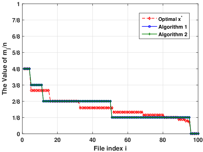
Fig. 7 compares the solution values of the obtained caching vector in different algorithms when , where the optimal solution of the continuous problem, Problem 2, is also included for comparison. It is seen that the solution of Algorithm 2 is identical to that of Algorithm 1. Fig. 7 also shows that more coded packets should be cached for more popular files, which justifies Theorem 1.
Remark 2.
In general, the encoding and decoding complexity of MDS codes or RLNC increases as the total number of fragments that each file is split into, i.e., , increases. However, the actual number of fragments that a file is split into does not have to be , depending on the optimized caching parameter . For example, we have for file from Fig. 7. Then, only needs to be split into fragments for encoding and each SBS stores one coded packet. Also, we have for file . Then, only needs to be split into fragments for encoding and each SBS stores one coded packet.
From the above results, we conclude that Algorithm 2 achieves almost the same performance as Algorithm 1 but with much lower complexity, especially for large and . Nevertheless, we still use Algorithm 1 for the AFOT maximization in the rest of this section since it obtains the globally optimal solution with manageable complexity.
V-C Effects of coding parameter
Fig. 8 depicts the AFOT performance with respect to different when the cache size varies. In the special case with , the coded caching reduces to uncoded caching which only stores the most popular files in each SBS, namely , for , and , for . It is seen from Fig. 8 that the AFOT increases dramatically when increases from to but the gain diminishes quickly when reaches . When , the performance is very close to the upper bound determined the optimal solution of Problem 2. Note that the coding parameter is the maximum possible number of decoding layers for SIC receiver and hence determines the maximum receiver complexity. It also affects the computational complexity of Algorithm 1 as shown in Fig. 7. Thus, cannot be too large in practical systems. The results in Fig. 8 suggest that it is good enough to let . In the rest of this section, we fix when considering the AFOT performance.

V-D Coded Caching vs. Uncoded Caching on AFOT
We show the performance of coded caching in comparison with uncoded caching on the AFOT under different parameter settings. Two uncoded caching schemes are considered as benchmarks, namely most popular caching (MPC) and optimal probabilistic caching (OPC).
V-D1 Most Popular Caching (MPC)
This is the special case of coded caching when . Specifically, we store the most popular files in each SBS. If requests any of these cached files, it only connects with the nearest SBS. If the transmission of the nearest SBS is successful, the user request is satisfied. If not, retrieves the file from an MBS. If requests any of the other uncached files, the file will be transmitted directly by the MBS. Therefore, the AFOT, denoted as , can be calculated as .
V-D2 Optimal Probabilistic Caching (OPC)
In the probabilistic caching strategy, each SBS caches independently with probability . The vector is referred to as the caching probability vector with constraints as . When a user submits a request for , it will be associated with the strongest SBS (in terms of the average received signal strength) that has cached the file. The probability vector can be optimized to maximize the AFOT. Note that this problem has been studied in [14]. We refer readers to [14, Theorem 3].

Fig. 9 illustrates the AFOT performance with respect to cache size . It is observed that the proposed coded caching scheme performs significantly better than the two benchmarks. This is because coded caching can fully exploit the accumulated cache size in the network. MPC, on the other hand, only enjoys the local caching gain since the same contents are cached in each SBS. OPC improves upon MPC by exploiting the randomness in the probabilistic caching but the gain is limited.

Fig. 10 illustrates the AFOT performance with respect to Zipf parameter . It is again observed that coded caching has much better performance than MPC and OPC, especially when is small . In the high region , most of the user requests are for the few popular files in . Both coded caching and OPC degenerate to MPC, which matches with the finding in Corollary 2.

In Fig. 11, we illustrate the AFOT performance with respect to the target SIR threshold . In the small region, coded caching has much better performance due to that the accumulated cache size of the nearest SBSs are used to store different contents. When increases, the performances of coded and uncoded caching schemes all converge as expected from Corollary 2. This is because when is large, the successful transmission probability for the nearest SBS in coded caching is low as shown in Fig. 2. As a result, the chance for the SIC-based receiver to decode the second or higher order signal is much lower. Thus, the accumulated cache size cannot be fully exploited by coded caching. In fact, for both coded caching and OPC, most of the cache size in each SBS is used to store the most popular contents when the successful transmission probability for the nearest SBS has been low.
V-E Coded Caching vs. MPC on AER

Finally, in Fig. 12, we illustrate the AER performance of coded caching in comparison with the conventional MPC at different Zipf parameter and different cache size . The optimal solution of Problem 3, the coded cache problem for AER maximization, obtained via exhaustive search is also presented for comparison. It is first seen that Algorithm 3, the proposed heuristic algorithm to solve Problem 3, performs almost identical to the optimal solution. It is then seen that coded caching outperforms MPC when , i.e., the file popularity distribution is close to uniform, but the gain vanishes when . This is because the ergodic rate of each file (if cached) in coded caching is determined by the worst SIR among all decoding layers as defined in (7) while the ergodic rate of each file (if cached) in MPC is always determined the nearest SBS. As such, when the Zipf parameter is large, the gain from the high cache hit as a result of exploiting the accumulated cache size in coded caching is not enough to compensate the rate loss due to SIC receiver. Thus, coded caching will degenerate to MPC when the file popularity distribution is non-uniform.
VI Conclusions
In this paper, we investigated the optimal coded caching in cache-enabled SCNs. We proposed a content delivery framework for coded caching where multiple SBSs transmit concurrently upon a user request and the user decodes independent coded packets from these SBSs with SIC-based receiver. We obtained a closed-form expression for the success probability of each decoding layer with SIC receiver in the high SNR region and a closed-form expression of the average fractional offloaded traffic. We also obtained a tractable expression of the average ergodic rate. Then, a greedy-based optimal algorithm was proposed to solve the cache placement problem for AFOT maximization. We also obtained an upper bound assuming a limiting case that the files are split into infinite parts. Based on that, a low-complexity algorithm with high performance was proposed for the cache placement problem. To maximize AER, we formulated the coded cache problem as a standard MCKP and proposed a heuristic algorithm to solve it. Numerical results showed that coded caching with SIC receiver significantly outperforms uncoded caching in terms of AFOT performance at low SIR thresholds, even when number of segments for file splitting is small. It was shown that coded caching degenerates to MPC in terms of AER performance unless the file popularity distribution tends to be uniform.
Appendix A: Proof of Lemma 1
In general, ’s in (3) are correlated for different in the SIC receiver. To make the analysis more tractable, we assume that the events are independent for all as in [25]. As shown in Section V-A, ignoring such correlations has little effects on the system performance as in [25]. Hence, the successful transmission probability for the -th nearest SBS is
| (22) |
Here, is due to the independence assumption as in [25]; follows from [25, Lemma 3] by letting ; is due to the change of variable ; and is due to the change of variable . Note that the changes of variables in and are to convert the unbounded integral in to the definite integral, which is numerically more convenient.
Appendix B: Proof of Lemma 2
When , there is no packet of in each SBS. Therefore, FOT is equal to .
When , we have FOT as follows.
| (23) |
Appendix C: Proof of Lemma 4
When , , we have . Hence is a piece-wise linear function.
In each region , the derivative of can be obtained as
| (25) |
In (25), the last inequality holds due to the decreasing property of . Thus, is an increasing function.
Appendix D: Proof of Lemma 5
When , there is no packet of in each SBS, thus the ergodic rate is .
Appendix E: Proof of Theorem 1
We assume that there are two files in and file is more popular than file , i.e., . However, we assume that less packets of file is stored in each SBS than that of file , i.e., , which has maximized the AFOT performance. We have the sum of FOT for file and file as
| (28) |
Now, we try to store packets of file and packets of file . Thus, the sum of FOT for file and file can be calculated as
| (29) |
Then, we compare with
| (30) |
We have known that is an increasing sequence of . Therefore, . Then, we can get . That means if we store packets of file and packets of file , AFOT can be larger. Therefore, more popular files store more packets in cache.
Appendix F: Proof of Corollary 2
Let . For , is a decreasing function of . Define . We thus have
| (31) |
Since , . Thus, is an increasing function of . Overall, is a decreasing function of . If , there must exist a such that inequality (16) satisfies when . The first part of the Corollary is thus proven.
References
- [1] X. Xu and M. Tao, “Stochastic modeling, analysis and optimization of coded caching in small-cell networks,” to appear in 2017 IEEE International Conference on Communications (ICC). IEEE, 2017.
- [2] N. Golrezaei, A. F. Molisch, A. G. Dimakis, and G. Caire, “Femtocaching and device-to-device collaboration: A new architecture for wireless video distribution,” IEEE Communications Magazine, vol. 51, no. 4, pp. 142–149, April 2013.
- [3] E. Baştuğ, M. Bennis, and M. Debbah, “Living on the edge: The role of proactive caching in 5g wireless networks,” IEEE Communications Magazine, vol. 52, no. 8, pp. 82–89, 2014.
- [4] D. Liu, B. Chen, C. Yang, and A. F. Molisch, “Caching at the wireless edge: design aspects, challenges, and future directions,” IEEE Communications Magazine, vol. 54, no. 9, pp. 22–28, 2016.
- [5] M. A. Maddah-Ali and U. Niesen, “Fundamental limits of caching,” IEEE Transactions on Information Theory, vol. 60, no. 5, pp. 2856–2867, May 2014.
- [6] M. Tao, E. Chen, H. Zhou, and W. Yu, “Content-centric sparse multicast beamforming for cache-enabled cloud ran,” IEEE Transactions on Wireless Communications, vol. 15, no. 9, pp. 6118–6131, Sept 2016.
- [7] B. Zhou, Y. Cui, and M. Tao, “Stochastic content-centric multicast scheduling for cache-enabled heterogeneous cellular networks,” IEEE Transactions on Wireless Communications, vol. 15, no. 9, pp. 6284–6297, Sept 2016.
- [8] X. Peng, J. C. Shen, J. Zhang, and K. B. Letaief, “Joint data assignment and beamforming for backhaul limited caching networks,” in 2014 IEEE 25th Annual International Symposium on Personal, Indoor, and Mobile Radio Communication (PIMRC), Sept 2014, pp. 1370–1374.
- [9] D. Malak, M. Al-Shalash, and J. G. Andrews, “Optimizing content caching to maximize the density of successful receptions in device-to-device networking,” IEEE Transactions on Communications, vol. 64, no. 10, pp. 4365–4380, Oct 2016.
- [10] B. Dai and W. Yu, “Joint user association and content placement for cache-enabled wireless access networks,” in 2016 IEEE International Conference on Acoustics, Speech and Signal Processing (ICASSP). IEEE, 2016, pp. 3521–3525.
- [11] B. Blaszczyszyn and A. Giovanidis, “Optimal geographic caching in cellular networks,” in 2015 IEEE International Conference on Communications (ICC). IEEE, 2015.
- [12] D. Liu and C. Yang, “Caching policy toward maximal success probability and area spectral efficiency of cache-enabled hetnets,” arXiv preprint arXiv:1608.03749, 2016.
- [13] S. H. Chae and W. Choi, “Caching placement in stochastic wireless caching helper networks: Channel selection diversity via caching,” IEEE Transactions on Wireless Communications, vol. 15, no. 10, pp. 6626–6637, Oct 2016.
- [14] Y. Chen, M. Ding, J. Li, Z. Lin, G. Mao, and L. Hanzo, “Probabilistic small-cell caching: Performance analysis and optimization,” IEEE Transactions on Vehicular Technology, vol. PP, no. 99, pp. 1–1, 2016.
- [15] Z. Chen, J. Lee, T. Q. Quek, and M. Kountouris, “Cooperative caching and transmission design in cluster-centric small cell networks,” arXiv preprint arXiv:1601.00321, 2016.
- [16] K. Shanmugam, N. Golrezaei, A. G. Dimakis, A. F. Molisch, and G. Caire, “Femtocaching: Wireless content delivery through distributed caching helpers,” IEEE Transactions on Information Theory, vol. 59, no. 12, pp. 8402–8413, Dec 2013.
- [17] E. Baştuğ, M. Bennis, M. Kountouris, and M. Debbah, “Cache-enabled small cell networks: Modeling and tradeoffs,” EURASIP Journal on Wireless Communications and Networking, vol. 2015, no. 1, pp. 1–11, 2015.
- [18] C. Yang, Y. Yao, Z. Chen, and B. Xia, “Analysis on cache-enabled wireless heterogeneous networks,” IEEE Transactions on Wireless Communications, vol. 15, no. 1, pp. 131–145, Jan 2016.
- [19] V. Bioglio, F. Gabry, and I. Land, “Optimizing MDS codes for caching at the edge,” in 2015 IEEE Global Communications Conference (GLOBECOM), Dec 2015, pp. 1–6.
- [20] J. Liao, K. K. Wong, M. R. A. Khandaker, and Z. Zheng, “Optimizing cache placement for heterogeneous small cell networks,” IEEE Communications Letters, no. 99, 2016.
- [21] E. Altman, K. Avrachenkov, and J. Goseling, “Coding for caches in the plane,” arXiv preprint arXiv:1309.0604, 2013.
- [22] J. Gu, W. Wang, A. Huang, and H. Shan, “Proactive storage at caching-enable base stations in cellular networks,” in 2013 IEEE 24th Annual International Symposium on Personal, Indoor, and Mobile Radio Communications (PIMRC). IEEE, 2013.
- [23] A. Khreishah, J. Chakareski, and A. Gharaibeh, “Joint caching, routing, and channel assignment for collaborative small-cell cellular networks,” IEEE Journal on Selected Areas in Communications, vol. 34, no. 8, pp. 2275–2284, Aug 2016.
- [24] H. Kellerer, U. Pferschy, and D. Pisinger, Introduction to NP-Completeness of knapsack problems. Springer, 2004.
- [25] M. Wildemeersch, T. Q. S. Quek, M. Kountouris, A. Rabbachin, and C. H. Slump, “Successive interference cancellation in heterogeneous networks,” IEEE Transactions on Communications, vol. 62, no. 12, pp. 4440–4453, Dec 2014.