Micro-wave assisted transparency in a M-system

We consider a five level atomic M-system as shown in Fig. 1a. The electric field associated with the lasers driving the transition $|{i}\rangle$ $\rightarrow$ $|{i+1}\rangle$ is E${}_{i,i+1}e^{i(\omega^{L}_{i,i+1}t+\phi^{L}_{i,i+1})}$. The E_i,i+1 is amplitude, $\omega_{i,i+1}$ is the frequency and $\phi^{L}_{i,i+1}$ is the phase. We define Rabi frequency $\Omega_{i,j}=d_{i,j}E_{i,j}e^{i\phi^{L}_{i,j}}/\hbar$ for the transition $|{i}\rangle$ $\rightarrow$ $|{j}\rangle$ having the dipole moment matrix element $d_{i,j}$ driven by a laser with electric field amplitude E_i,j and the phase $\phi^{L}_{i,j}$ . The $\Omega_{12}$ is the Rabi frequency of the probe laser driving $|{1}\rangle$ $\rightarrow$ $|{2}\rangle$ and shown with solid blue arrow in Fig. 1. The Rabi frequencies of the control lasers driving the transitions $|{2}\rangle$ $\rightarrow$ $|{3}\rangle$, $|{3}\rangle$ $\rightarrow$ $|{4}\rangle$ and $|{4}\rangle$ $\rightarrow$ $|{5}\rangle$ are denoted by $\Omega_{23}$, $\Omega_{34}$ and $\Omega_{45}$ respectively and shown with solid red arrows. The lower level states $|{3}\rangle$ and $|{5}\rangle$ is coupled by a MW field with Rabi frequency $\Omega^{MW}_{35}$ as shown with solid green arrow. The M-system can be realized in ⁸⁷Rb at the D₁ line using the two hyperfine levels $F_{g}=1$ and $F_{g}=2$ of the ground state 5S_1/2 and the hyperfine level $F_{e}=1$ of excited state 5P_1/2 as shown in Fig. 1b. The decay rate of the excited state 5P_1/2 is $2\pi\times$6 MHz. We apply a large magnetic field to split the magnetic sublevels to keep away the unwanted sublevels from resonance and to define the quantization axis. The sign and value of the Lande g factor for the chosen hyperfine is suitable to split and keep away the unwanted transitions. At 200 G applied magnetic field the splitting of the magnetic sublevels for $F_{e}=1$ is 2$\pi\times$46 MHz and splitting for $F_{g}=2$ and $F_{g}=1$ is 2$\pi\times$140 MHz as shown in Fig. 1c. We consider the probe to be $\sigma^{-}$ polarized and driving the transition $|{F_{g}=2;m_{F}=+1}\rangle$ $\rightarrow$ $|{F_{e}=1;m_{F}=0}\rangle$. The $\pi$ polarized control laser is driving the $|{F_{g}=2;m_{F}=0}\rangle$ $\rightarrow$ $|{F_{e}=1;m_{F}=0}\rangle$ transition. The two $\sigma^{-}$ polarized control lasers are driving the $|{F_{g}=2;m_{F}=0}\rangle$ $\rightarrow$ $|{F_{e}=1;m_{F}=-1}\rangle$ and $|{F_{g}=1;m_{F}=0}\rangle$ $\rightarrow$ $|{F_{e}=1;m_{F}=-1}\rangle$ transitions as shown in Fig. 1 c.

In the absence of the control lasers all the magnetic sublevels of the hyperfine states $F_{g}=1$ and $F_{g}=2$ will be equally populated. However when the control lasers are applied, the population in the ground states connected with the control lasers will deplete. In the steady state there will be no population left in the $|{F_{g}=1,m_{F}=0}\rangle$ and $|{F_{g}=2,m_{F}=0}\rangle$ states as shown in Fig. 1c.

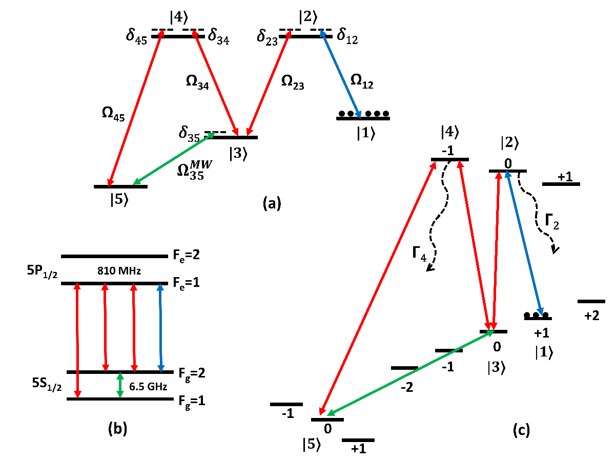
The unperturbed atomic Hamiltonian can be written as

where $\hbar\omega_{j}$ is the energy of the $|{j}\rangle$ state. Under the action of five coherent fields, the interaction Hamiltonian of the system in the dipole approximation is given by

Hence the total Hamiltonian will be $H=H_{0}+H_{I}$. We use suitable unitary transformation to eliminate the explicit time dependent part in the Hamiltonian. In rotating wave approximation, the effective interaction Hamiltonian can be expressed as

where $\delta_{12}=\omega^{L}_{12}-(\omega_{2}-\omega_{1})$, $\delta_{23}=\omega^{L}_{23}-(\omega_{2}-\omega_{3})$, $\delta_{34}=\omega^{L}_{34}-(\omega_{4}-\omega_{3})$, $\delta_{45}=\omega^{L}_{45}-(\omega_{4}-\omega_{5})$ and $\delta^{MW}_{35}=\omega^{MW}_{35}-(\omega_{5}-\omega_{3})$ known as detunings of the lasers for respective transitions. Now we impose the condition $\delta_{45}+\delta_{35}^{MW}-\delta_{34}=0$, so that the time dependence is completely eliminated from the effective interaction Hamiltonian. To explore the dynamics of the atomic system, we use the density matrix equations where radiative relaxation of the atomic states are included. The atomic density operator $\rho$ obey the following equations

where $\Gamma$ is the relaxation matrix [46].

To study the response of the medium, we numerically solve the density matrix equations at steady-state condition. We derive an analytical expression for the probe field response that is correct to first order in probe field approximation and exact for the all order in control fields. In this weak approximation, there will be no population transfer and hence the evolution of the population i.e. diagonal terms of the density matrix such as $\rho_{11}$, $\rho_{22}$, $\rho_{33}$, $\rho_{44}$ and $\rho_{55}$ can be ignored with $\rho_{11}\approx 1$, $\rho_{22}\approx 0$, $\rho_{33}\approx 0$, $\rho_{44}\approx 0$ and $\rho_{55}\approx 0$. Time evolution for the coherences i.e. off-diagonal terms of the density matrix will be given by following set of equations

where

The decay rate of the states $|{1}\rangle$, $|{2}\rangle$, $|{3}\rangle$, $|{4}\rangle$ and $|{5}\rangle$ are given by $\Gamma_{1}$, $\Gamma_{2}$, $\Gamma_{3}$, $\Gamma_{4}$ and $\Gamma_{5}$, respectively. Again within the same weak probe limit, the coherences $\rho_{23}$ $\approx$$\rho_{24}$$\approx$$\rho_{25}$$\approx$0. Under the steady state condition i.e. $\dot{\rho}_{ij}=0$, the equations (5) become

We obtain following analytical expression for $\rho_{12}$ by solving above linear algebraic equations

where $\phi=\phi^{MW}_{35}-\phi^{L}_{34}-\phi^{L}_{45}$. In order to ensure the correctness of the above approximation, in Fig.(2) we plot the normalized absorption of the probe field (Im($\rho_{12}$)$\Gamma_{2}/\Omega_{12}$) as a function of normalized probe detuning ($\delta_{12}/\Gamma_{2}$) obtain from analytical expression of $\rho_{12}$ as given in Eq.(7) as well as the complete numerical solution of density matrix equation as stated in Eq.(4). It is clear from Fig.(2) that the complete numerical results are in an excellent agreement with the approximated analytical solutions.

In this section, we study the effect of the MW field on the lineshape of the probe absorption. We consider all the control and MW fields are on the resonance. First we discuss the role of individual control fields one by one and finally the MW field. There is a broad Lorentzian profile having a full width at half maximum of $\Gamma_{2}$ which is $2\pi\times$ 6 MHz in this case [7, 8]. At the line centre of the Lorentzian profile, the probe response develops a sharp EIT dip in the presence of the control field $\Omega_{23}$ [7, 36]. The linewidth of EIT dip depends decoherence rates and the control field intensity $|\Omega_{23}|$ and can be expressed as $\Delta\omega\propto|\Omega_{23}|^{2}/4\Gamma_{2}$ [47]. Here we have taken $\Gamma_{1}$=$\Gamma_{3}$=0, as states $|{1}\rangle$ and $|{3}\rangle$ are the ground states. The control laser $\Omega_{34}$ recovers the absorption against EIT and known as EITA has been discussed in details in our previous work [36]. When $|\Omega_{34}|<|\Omega_{23}|$ the linewidth of EITA peak is comparable with the linewidth of EIT dip and it is broadening with the increase of the $\Omega_{34}$. Finally when $|\Omega_{34}|>|\Omega_{23}|$ the linewidth of the EITA peak will be $\Gamma_{2}$. In the presence of the control laser $\Omega_{45}$ there will be transparency against EITA, known as EITAT and has also been discussed in our previous work [36]. The linewidth of the EITAT is given by the expression,

$\Delta\omega\propto\frac{|\Omega_{23}||\Omega_{45}|}{4\Gamma_{2}\left[(|\Omega_{34}|^{2}+|\Omega_{45}|^{2})\left(\frac{1}{|\Omega_{23}|^{2}}+\frac{1}{|\Omega_{45}|^{2}}+\frac{|\Omega_{34}|^{2}}{|\Omega_{23}|^{2}|\Omega_{45}|^{2}}\right)-1\right]}$

The linewidth of the EITAT is modulated by the three control field intensities $\Omega_{23}$, $\Omega_{34}$, $\Omega_{45}$ and the decay rate of the excited states $|{2}\rangle$, $|{4}\rangle$. Here we have taken $\Gamma_{5}$=0, as state $|{5}\rangle$ is the metastable ground state. The MW field, $\Omega^{MW}_{35}$ splits or shifts the EITAT dip, depending upon the phase $\phi$ as below as shown in Fig. 3.

Fig. 3 shows the plot for normalized absorption (Im($\rho_{12})\Gamma_{2}/\Omega_{12}$) vs probe detuning in the unit of ($\Gamma_{2}$) for various combination of the phase and the MW field strength. In Fig. 3a for $\phi$=0 there is shift of EITAT dip by approximately $\frac{|\Omega^{MW}_{35}|}{2}$ to the right while it shifts to the left by same amount for $\phi$=$\pi$. For the $\phi=\pi/2$ there is broadening and reduction of the EITAT dip. However with the relatively high value of the MW field, $|\Omega^{MW}_{35}|$=$2\pi\times$0.3 MHz there is further reduction of EITAT dip and splitting increases and visible as shown in Fig. 3b.

The variation of the normalized probe absorption as a function of the MW Rabi frequency, $|\Omega^{MW}_{35}|$ in unit of $\Gamma_{2}$ is shown in Fig. 4. As in the presence of the MW field the EITAT dip shift, thus with increase of the MW Rabi frequency the absorption increases and saturates to 1. The slope of the absorption profile depends upon the EITAT linewidth, and the narrower will be the linewidth sharper will be the slope. As we see in Fig. 4 the red solid curve shows the sharper rise in the absorption with the MW Rabi frequency as compared to the dashed green curve. This is because the EITAT dip linewidth is power broadened by the control laser with higher Rabi frequency. The red solid curve saturates faster as compare to the dotted blue curve this is because with $\phi=\pi/2$ the EITAT dip splits instead of shifting and hence will have lower slope as compare to the $\phi=0$ with same Rabi frequency of the control lasers.

References

- [1] J. A. Sedlacek, A. Schwettmann, H. Kübler, and J. P. Shaffer, Phys. Rev. Lett. 111, 063001 (2013), URL http://link.aps.org/doi/10.1103/PhysRevLett.111.063001.
- [2] J. A. Sedlacek, A. Schwettmann, H. Kubler, R. Low, T. Pfau, and J. P. Shaffer, Nature physics 8, 819 (2012), URL http://link.aps.org/doi/10.1103/PhysRevLett.111.063001.
- [3] Y. Jiao, Z. Yang, J. Li, G. Raithel, J. Zhao, and S. Jia, ArXiv e-prints (2016), eprint 1601.01748.
- [4] M. Fleischhauer, A. Imamoglu, and J. P. Marangos, Rev. Mod. Phys. 77, 633 (2005), URL http://link.aps.org/doi/10.1103/RevModPhys.77.633.
- [5] B. Peng, S. K. Ozdemir, W. Chen, F. Nori, and L. Yang, Nature 5 (2014), URL http://www.nature.com/articles/ncomms6082.
- [6] O. S. Mishina, M. Scherman, P. Lombardi, J. Ortalo, D. Felinto, A. S. Sheremet, A. Bramati, D. V. Kupriyanov, J. Laurat, and E. Giacobino, Phys. Rev. A 83, 053809 (2011), URL http://link.aps.org/doi/10.1103/PhysRevA.83.053809.
- [7] S. M. Iftiquar, G. R. Karve, and V. Natarajan, Phys. Rev. A 77, 063807 (2008), URL http://link.aps.org/doi/10.1103/PhysRevA.77.063807.
- [8] S. M. Iftiquar and V. Natarajan, Phys. Rev. A 79, 013808 (2009), URL http://link.aps.org/doi/10.1103/PhysRevA.79.013808.
- [9] D. Budker, D. F. Kimball, S. M. Rochester, and V. V. Yashchuk, Phys. Rev. Lett. 83, 1767 (1999), URL http://link.aps.org/doi/10.1103/PhysRevLett.83.1767.
- [10] H. Wang, D. Goorskey, and M. Xiao, Phys. Rev. Lett. 87, 073601 (2001), URL http://link.aps.org/doi/10.1103/PhysRevLett.87.073601.
- [11] D. F. Phillips, A. Fleischhauer, A. Mair, R. L. Walsworth, and M. D. Lukin, Phys. Rev. Lett. 86, 783 (2001), URL http://link.aps.org/doi/10.1103/PhysRevLett.86.783.
- [12] T. N. Dey and G. S. Agarwal, Phys. Rev. A 67, 033813 (2003), URL http://link.aps.org/doi/10.1103/PhysRevA.67.033813.
- [13] S. Menon and G. S. Agarwal, Phys. Rev. A 61, 013807 (1999), URL http://link.aps.org/doi/10.1103/PhysRevA.61.013807.
- [14] A. Lazoudis, T. Kirova, E. H. Ahmed, P. Qi, J. Huennekens, and A. M. Lyyra, Phys. Rev. A 83, 063419 (2011), URL http://link.aps.org/doi/10.1103/PhysRevA.83.063419.
- [15] C. Zhu, C. Tan, and G. Huang, Phys. Rev. A 87, 043813 (2013), URL http://link.aps.org/doi/10.1103/PhysRevA.87.043813.
- [16] A. Krishna, K. Pandey, A. Wasan, and V. Natarajan, EPL (Europhysics Letters) 72, 221 (2005), URL http://stacks.iop.org/0295-5075/72/221.
- [17] J. D. Pritchard, D. Maxwell, A. Gauguet, K. J. Weatherill, M. P. A. Jones, and C. S. Adams, Phys. Rev. Lett. 105, 193603 (2010), URL http://link.aps.org/doi/10.1103/PhysRevLett.105.193603.
- [18] A. V. Gorshkov, J. Otterbach, M. Fleischhauer, T. Pohl, and M. D. Lukin, Phys. Rev. Lett. 107, 133602 (2011), URL http://link.aps.org/doi/10.1103/PhysRevLett.107.133602.
- [19] H. Gorniaczyk, C. Tresp, J. Schmidt, H. Fedder, and S. Hofferberth, Phys. Rev. Lett. 113, 053601 (2014), URL http://link.aps.org/doi/10.1103/PhysRevLett.113.053601.
- [20] H.-R. Noh and H. S. Moon, Phys. Rev. A 92, 013807 (2015), URL http://link.aps.org/doi/10.1103/PhysRevA.92.013807.
- [21] S. Jin, Y. Li, and M. Xiao, Optics Communications 119, 90 (1995), ISSN 0030-4018, URL http://www.sciencedirect.com/science/article/pii/003040189500362C.
- [22] S. Das, A. Grankin, I. Iakoupov, E. Brion, J. Borregaard, R. Boddeda, I. Usmani, A. Ourjoumtsev, P. Grangier, and A. S. Sørensen, Phys. Rev. A 93, 040303 (2016), URL http://link.aps.org/doi/10.1103/PhysRevA.93.040303.
- [23] S. R. de Echaniz, A. D. Greentree, A. V. Durrant, D. M. Segal, J. P. Marangos, and J. A. Vaccaro, Phys. Rev. A 64, 013812 (2001), URL http://link.aps.org/doi/10.1103/PhysRevA.64.013812.
- [24] D. Han, H. Guo, Y. Bai, and H. Sun, Physics Letters A 334, 243 (2005), ISSN 0375-9601, URL http://www.sciencedirect.com/science/article/pii/S0375960104016202.
- [25] M. G. Bason, A. K. Mohapatra, K. J. Weatherill, and C. S. Adams, Journal of Physics B: Atomic, Molecular and Optical Physics 42, 075503 (5pp) (2009), URL http://stacks.iop.org/0953-4075/42/075503.
- [26] C. Goren, A. D. Wilson-Gordon, M. Rosenbluh, and H. Friedmann, Phys. Rev. A 69, 053818 (2004), URL http://link.aps.org/doi/10.1103/PhysRevA.69.053818.
- [27] Y. Chen, X. G. Wei, and B. S. Ham, Journal of Physics B: Atomic, Molecular and Optical Physics 42, 065506 (2009), URL http://stacks.iop.org/0953-4075/42/i=6/a=065506.
- [28] S. R. Chanu, A. K. Singh, B. Brun, K. Pandey, and V. Natarajan, Optics Communications 284, 4957 (2011), ISSN 0030-4018, URL http://www.sciencedirect.com/science/article/pii/S0030401811007127.
- [29] X.-D. Tian, Y.-M. Liu, X.-B. Yan, C.-L. Cui, and Y. Zhang, Optics Communications 345, 6 (2015), ISSN 0030-4018, URL http://www.sciencedirect.com/science/article/pii/S0030401815000656.
- [30] D. Yan, Y.-M. Liu, Q.-Q. Bao, C.-B. Fu, and J.-H. Wu, Phys. Rev. A 86, 023828 (2012), URL http://link.aps.org/doi/10.1103/PhysRevA.86.023828.
- [31] T. Hong, C. Cramer, W. Nagourney, and E. N. Fortson, Phys. Rev. Lett. 94, 050801 (2005).
- [32] K. Pandey, D. Kaundilya, and V. Natarajan, Optics Communications 284, 252 (2011), ISSN 0030-4018, URL http://www.sciencedirect.com/science/article/pii/S0030401810008862.
- [33] S. Kumar, T. Lauprêtre, R. Ghosh, F. Bretenaker, and F. Goldfarb, Phys. Rev. A 84, 023811 (2011), URL http://link.aps.org/doi/10.1103/PhysRevA.84.023811.
- [34] S. Kumar, T. Lauprêtre, F. Bretenaker, F. Goldfarb, and R. Ghosh, Phys. Rev. A 88, 023852 (2013), URL http://link.aps.org/doi/10.1103/PhysRevA.88.023852.
- [35] Y.-X. Hu, C. Miniatura, D. Wilkowski, and B. Grémaud, Phys. Rev. A 90, 023601 (2014), URL http://link.aps.org/doi/10.1103/PhysRevA.90.023601.
- [36] K. Pandey, Phys. Rev. A 87, 043838 (2013), URL http://link.aps.org/doi/10.1103/PhysRevA.87.043838.
- [37] M. Khazali, K. Heshami, and C. Simon, Phys. Rev. A 91, 030301 (2015), URL http://link.aps.org/doi/10.1103/PhysRevA.91.030301.
- [38] G. S. Agarwal, T. N. Dey, and S. Menon, Phys. Rev. A 64, 053809 (2001), URL http://link.aps.org/doi/10.1103/PhysRevA.64.053809.
- [39] H. Li, V. A. Sautenkov, Y. V. Rostovtsev, G. R. Welch, P. R. Hemmer, and M. O. Scully, Phys. Rev. A 80, 023820 (2009), URL http://link.aps.org/doi/10.1103/PhysRevA.80.023820.
- [40] M. Manjappa, S. S. Undurti, A. Karigowda, A. Narayanan, and B. C. Sanders, Phys. Rev. A 90, 043859 (2014), URL http://link.aps.org/doi/10.1103/PhysRevA.90.043859.
- [41] R. K. V., T. N. Dey, S. Das, and P. K. Jha, Opt. Lett. 40, 2229 (2015), URL http://ol.osa.org/abstract.cfm?URI=ol-40-10-2229.
- [42] A. Eilam, A. D. Wilson-Gordon, and H. Friedmann, Opt. Lett. 34, 1834 (2009), URL http://ol.osa.org/abstract.cfm?URI=ol-34-12-1834.
- [43] D. V. Kosachiov, B. G. Matisov, and Y. V. Rozhdestvensky, Journal of Physics B: Atomic, Molecular and Optical Physics 25, 2473 (1992), URL http://stacks.iop.org/0953-4075/25/i=11/a=005.
- [44] N. Radwell, T. W. Clark, B. Piccirillo, S. M. Barnett, and S. Franke-Arnold, Phys. Rev. Lett. 114, 123603 (2015), URL http://link.aps.org/doi/10.1103/PhysRevLett.114.123603.
- [45] M. D. Lukin, Rev. Mod. Phys. 75 (2003), URL http://link.aps.org/doi/10.1103/RevModPhys.75.457.
- [46] M. O. Scully and M. S. Zubairy, Quantum Optics: (Cambridge University Press, Cambridge, 1997), ISBN 9780511813993, URL https://www.cambridge.org/core/books/quantum-optics/08DC53888452CBC6CDC0FD8A1A1A4DD7.
- [47] M. Fleischhauer and M. D. Lukin, Phys. Rev. A 65, 022314 (2002), URL http://link.aps.org/doi/10.1103/PhysRevA.65.022314.